
Household Wealth: Low-Yielding and Poorly Structured?

1
HFU Business School, Furtwangen University, 78054 Schwenningen, Germany
2
Muenster School of Business, FH Muenster, 48143 Muenster, Germany
*
Author to whom correspondence should be addressed.
J. Risk Financial Manag. 2021, 14(3), 99; https://0-doi-org.brum.beds.ac.uk/10.3390/jrfm14030099
Submission received: 25 January 2021
/
Revised: 23 February 2021
/
Accepted: 24 February 2021
/
Published: 3 March 2021
(This article belongs to the Special Issue Household Finance)
Abstract
:In this paper, we present a newly generated data set on real returns of households’ aggregated asset holdings, which adds additional and more sophisticated information to existing relevant datasets in the literature. To do this, we draw on various datasets from public and private sources and then transform and combine them in a consistent manner that allows for international comparative and intertemporal analyses. Based on this, we address two current debates on the development of household wealth in the euro area that have been triggered by the low-interest environment. The first debate refers to the development of real yields on household wealth from 2000 to 2018, whereas the second debate deals with the mean-variance efficiency of household portfolios. Contrary to widespread belief, we find that yields on total wealth, which were largely dominated by non-financial assets’ yields, were mostly positive, although they exhibit a declining trend. Moreover, on average, overall real yields were significantly lower after 2008. Referring to portfolio efficiency, we find that current portfolios seem to be comparatively close to mean-variance efficiency. If households were to optimize their portfolios despite limited room for improvement, holdings of equity and investment fund shares should be reduced, contradicting common recommendations of financial advisors.
1. Introduction
Since the outbreak of the financial crisis in 2008, with one brief exception in 2011, there has been only one direction for key interest rates in the eurozone: downwards. Moreover, there are currently no signs of a “normalization” of key interest rates to pre-crisis levels. On the contrary: The turnaround in key interest rates has been postponed again and again. To combat the COVID-19 pandemic, central banks around the world took even more measures in 2020 to ensure the supply of liquidity and favorable financing conditions. Among others, the Eurosystem introduced an additional net asset purchase program (Pandemic Emergency Purchase Program (PEPP)) with a volume of at least €1850 billion (European Central Bank 2020a, 2020b, 2020c). Hence, it is very likely that official interest rates will remain low for the time being, also because any increases in key interest rates have been tied to numerous conditions (The debate on the economic causes of low (real) interest rates is intense and ongoing. Recent contributions include Lukasz and Smith (2017), Christensen and Rudebusch (2019), and Glick (2020). Several factors are at play on both the demand and supply sides, including excess savings in emerging markets, changes in income distribution, and more depressed investment demand. Demographics are thought by many to play a special role in this; Goodhart and Pradhan (2020) specifically address this. For the purpose of this paper, however, this debate is of minor importance and is, therefore, not considered).
Against this background, a heated debate has been sparked on the effects of the low-interest rate environment on household wealth in the eurozone, where the arguments run in two different directions. First, there is great dispute respecting the impact on the development of the overall real rate of return on household wealth (hereinafter referred to as the “level debate”). While some authors speak of an “expropriation of the saver” due to low or even negative real interest rates on deposits (Heise 2016), others emphasize the wealth- and return-increasing effects of rising asset prices for marketable assets (Bindseil et al. 2015). While this controversial debate has been initially focused on German households’ yields, it has meanwhile spread as well to other euro area countries.
Second, it has been claimed that households’ portfolios are inefficiently structured in terms of risk and return, as they contain a very high proportion of safe and low-yielding assets (hereinafter referred to as the “efficiency debate”). In principle, this efficiency debate has been around for a long time. Households’ preference for safe and low-yielding assets is usually attributed to a lack of financial literacy and/or a pronounced risk aversion—especially in Germany (Barasinska et al. 2011; Deuflhard et al. 2019). Occasionally, too high costs for greater diversification, too little trust in financial institutions, or one-sided advice from financial advisors are also blamed (Badarinza et al. 2016). Hence, far, policymakers in most countries have responded to this primarily by imposing stricter requirements on financial advice (e.g., documentation requirements) and by introducing special support instruments for certain asset classes (e.g., premiums). In practice, however, these instruments have so far mostly proved to be ineffective (Engen et al. 1996; Corneo et al. 2009). As a result, household portfolios are still largely considered inefficient today. Rupprecht (2020) has shown that households in the large euro area countries indeed have a high preference for safe assets, with little change in this preference over time. The low-interest phase has given additional impetus to this debate, as safe assets’ returns have declined mostly further since 2008; calls in favor of increasing the share of higher-yielding assets to improve the overall performance and efficiency of the household portfolio are growing louder (see, for instance, Jacobs et al. 2014).
This paper addresses both debates. For this purpose, it develops and analyses a dataset on the real rates of return on the total non-financial and financial wealth of households in the four large euro area countries (Germany, France, Italy, Spain) and in the euro area as a whole for the period 2000 to 2018.
This dataset is—to the best of our knowledge—unique to date as it goes beyond the scope of the previously available information in at least two ways. First, this concerns the level of economic agents we consider. Previous approaches typically focus on the national level. For instance, Piketty and Zucman (2014) estimate the aggregate wealth-to-income ratio for eight countries, covering a very long time span of more than three centuries. Although this is undoubtedly a major contribution, the authors only consider national wealth overall. The same holds true for Jorda et al. (2019). They extent the approach of Piketty and Zucman (2014) by additional countries and, more important, by building a bridge between different perspectives (national accounts, on one hand, finance and the long-run return of different asset types on the other) in order to improve previous estimates of asset returns. However, their comparative analysis is also limited to national balance sheets over time. Although these results are useful for comparing the level and dynamics of real returns in the low-interest-rate environment of the 2010s with earlier episodes, they do not allow to address the aforementioned debates on the particular effects for households. Since the structure and dynamics of household wealth typically differ from national wealth, this is an important shortcoming of existing research, in particular for the purpose of this paper.
On the other hand, the set of asset types we consider is also much broader and more differentiated than in most parts of the literature. For instance, while Dimson et al. (2009) provided pioneering work regarding the long-term development of investment returns, their approach includes only securities, leaving out all other kinds of assets. Since securities (i.e., bonds, equities and mutual fund shares)—so far—typically account for only a small share of households’ portfolios, the view is far too narrow to adequately address the above debates. Given the significant role of non-financial assets, a number of studies in recent years have attempted to shed more light on the evolution of housing wealth and its returns over time. Examples include Knoll et al. (2017), who provide information on house prices and returns (including rents) on the global level, and Duca et al. (forthcoming) with a comprehensive overview of the determinants of house price movements over time. However, certain assets are rarely taken into account. This is particularly true when it comes to determining their returns in an internationally comparable manner. Affected by this are, for example, claims against insurance companies. They are occasionally taken into account in national analyses (e.g., Deutsche Bundesbank 2015). To the best of our knowledge, however, there are no current analyses comparing different countries over time. This is unfortunate, given that insurance claims often contribute a large share to households’ (financial) wealth (Rupprecht 2020). The study of Badarinza et al. (2016) is one of the few that considers a broad and differentiated set of assets, including financial and non-financial wealth. However, it focuses on the composition of portfolios and their determinants without particularly addressing the role of real returns and their development over time.
In our paper, we overcome these shortcomings. The dataset we develop has a particular focus on households and covers a total of six different asset categories: (1) non-financial assets (consisting of fixed assets and land), (2) currency and deposits, securities (i.e., (3) debt securities, (4) equity holdings in the form of listed and unlisted shares, and (5) investment fund shares), as well as (6) claims against insurances. When determining the respective real yields, we go even further by taking into account, for example, different maturities, notice periods or issuers in the households’ portfolio in order to determine their yields as accurately as possible. Our starting point is the aforementioned study by Deutsche Bundesbank (2015), which is one of the few to carry out the development of the real return on financial assets of German households, taking into account all relevant asset classes.
Regarding the efficiency debate, our analysis adds to existing approaches in three ways. First, portfolio efficiency tests are typically conducted for individual investors or groups and individual assets or asset classes (e.g., Canner et al. 1997; Jacobs et al. 2014; Benartzi and Thaler 2001, 2007). Our approach, however, tests aggregated portfolios of complete household sectors and includes all assets held by households based on national accounts data. Second, while usual efficiency tests are mostly restricted to traded financial instruments, our approach additionally includes real estate and nontraded financial instruments like insurance and pension fund products. Third, to the best of our knowledge, no such analysis has yet been carried out so far for households in the major euro area countries and for the euro area household sector as a whole.
Based on this, we deal with three core questions. First, how did real returns on total, financial and non-financial assets develop over time from 2000 to 2018 (level debate)? Second, does the evolution of average real returns in the “pre-crisis phase” (2000–2007) differ from that in the “crisis and low-interest phase” (2008–2018) and, if so, how (level debate)? Moreover, third, can current portfolio allocations in 2018 be considered as efficient in terms of Markowitz’s mean-variance approach (Markowitz 1952, 1959) and in comparison to simple common heuristic portfolio allocation strategies, or should portfolios be adjusted (efficiency debate)?
Our key results are as follows: As to research question one, the results show that real returns on total household wealth were mostly positive in all jurisdictions but followed a declining trend and were driven mainly by real returns on non-financial assets. Referring to research question two, average real returns on total wealth were significantly lower between 2008 and 2018 than between 2000 and 2007 in all countries except for Germany; the reductions were mainly caused by drops in real yields (price effect), while portfolio shifts (volume effect) played a subordinate role. The negative price effects were dominated by diminishing real returns on non-financial wealth, which, however, remained the mainstay of real returns on total wealth. Addressing research question three, we find that the potentials for increasing real returns and/or decreasing risk by portfolio restructuring are very limited, as household portfolios seem to be close to their mean-variance optima. If households still want to optimize their portfolios according to a mean-variance framework, they should mostly follow a strategy that is against the common recommendation of financial advisors, namely, to reduce the share of equities and investment fund shares. Furthermore, by and large, the potential for increasing portfolio performance when following heuristic rules as well is very limited.
The paper is organized as follows: Section 2 explains the approach used to compute the aforementioned dataset. Section 3 ties in with the level debate by presenting and analyzing the data on real returns on household wealth, thereby addressing questions one and two above. Finally, Section 4 addresses the efficiency debate outlined above and thus the third question. To this end, it uses the data on the real returns and applies a classical Markowitz- and a heuristic portfolio analysis to the aggregated household portfolios in all countries under consideration. Section 5 concludes.
2. A New Dataset on Real Returns of Households’ Wealth—Computation Method and Inputs
As already mentioned, Deutsche Bundesbank (2015) was the first to order and weigh the arguments above by computing the real yield German households have earned on their financial wealth since the introduction of the euro. It is, therefore, natural to take this study as the starting point for our analysis in this paper.
The calculation of the Bundesbank study, which is described in more detail in Annuß and Rupprecht (2016), is regularly updated on a quarterly basis and published on the Bundesbank’s website. In order to be able to study the topic from a broader euro area perspective, Radke and Rupprecht (2018, 2019) expanded the Bundesbank’s approach by computing real yields on households’ financial wealth in the major euro area countries (Germany, France, Italy, Spain), and for the euro area as a whole from 2000 to 2017. This extension required a computational approach, which differed from Bundesbank’s calculations, mainly due to data limitations and access restrictions in some of the countries. Therefore, Radke and Rupprecht (2018, 2019) developed an alternative approach. Although their approach differs from the Bundesbank’s pioneering work, the Bundesbank’s data for Germany could be reproduced quite well, both with regard to the dynamics and levels (See, in particular, Figure 1 in Radke and Rupprecht (2018, p. 108), for a comparison with the Bundesbank data). This successful quality and consistency check was used as evidence for the appropriateness of the modified approach and applied to all other large euro area countries and the euro area as a whole. Furthermore, in 2019, the central bank of Austria published for the first time data on Austrian households’ real returns on financial assets (Oesterreichische Nationalbank 2019). The methodology is fairly comparable with the approaches mentioned above, and so are the results. To the best of our knowledge, other approaches for the compilation of real yields on households’ financial assets in the euro area currently do not exist (Andreasch et al. (2020) combined macroeconomic information on the real returns to households’ financial assets in Germany and Austria with microeconomic information on the portfolio composition of households with different wealth levels. Contrary to popular belief, they find that richer households are more adversely affected by the low-interest-rate environment than poorer households, at least in relative terms. In this context, the trend is generally more pronounced in Austria than in Germany, albeit at a fundamentally lower level of returns).
A major disadvantage of all approaches has so far been the neglect of non-financial assets. The main reason for this was the lack of availability of comparable data both in terms of data on stocks and their respective returns. This lack is problematic, however, as non-financial assets typically account for a large part of household wealth (60–70%). A profound assessment of the returns that households achieve with all their assets in times of low-interest rates, therefore, requires the consideration of non-financial assets. This is also true because the prices for dwellings, a key component of non-financial assets’ return, have developed very differently and at times very dynamically in the respective countries since the founding of monetary union.
For the purpose of this paper, the real return on households’ total assets was calculated for each country in a multi-stage process. First, the nominal return on each individual asset i in country j at time t, , was determined. Then, these country-specific individual nominal asset returns were transformed into real ex-post returns at time t, , by using country-specific realized or ex-post inflation rates at time t, , in accordance with the “exact” calculation method based on the relationship:
In the final step, the country-specific real yields of the individual assets were weighted with their respective national portfolio shares at time t, , and added up to the real total portfolio yield for each country j at time t, , according to the relationship:
where for all t and each country j.
The country-specific portfolio weights of the individual assets at time t, , were calculated as the ratio of the market value of each asset i in country j at time t, , to the market value of the total portfolio (sum of all national assets) of country j at time t, . Formally:
The countries considered were France, Germany, Italy, Spain and the euro area as a whole . Regarding the types of assets covered, the present computation approach follows the definitions of the European System of Accounts 2010 (ESA 2010) (ESA 2010 is the European counterpart of the System of National Accounts 2008 (SNA 2008) (United Nations 2010), which is the worldwide accounting standard for the compilation of national accounts data) (European Commission 2013; European Central Bank 2014). Figure 1 lists the complete set of assets being constituents of an aggregated household sector balance sheet according to the definitions of ESA 2010. The present computational approach, however, could not take into account all ESA 2010 assets and their respective yields for the reasons mentioned below. Hence, all assets and their respective yields highlighted in italics in Figure 1 were omitted in the present computation.
With regard to non-financial assets, stock data published by the OECD and the European Central Bank (ECB) were available in a consistent manner only for (tangible) fixed assets and land for Germany, France, Italy and the euro area as a whole. Therefore, data for Spain had to be estimated mainly on the basis of accumulated fixed capital information (net) in Spain; data on land was derived from ECB information on the euro area. The stocks of fixed assets officially published comprise the net capital stock valued at written-down replacement costs, i.e., at current prices, purchasers would need to pay less accumulated depreciation on those goods. This valuation method, as set out in ESA 2010, serves as a measure of the current market value of most fixed assets (It must be noted, however, that the net capital stock’s current replacement costs, as reported in the statistics and used as weights in the present compilation, can be quite different from the actual market prices for those goods. The ratio between the net capital stock’s current market price MP and its replacement cost RP defines Tobin’s q as q = MP/RP, determining the desired rate of growth of the capital stock, i.e., net investment (Tobin 1969b; Tobin and Brainard 1968, 1977). If q > 1, net investment is positive as buying new capital goods at replacement costs is cheaper than buying already existing capital goods in markets for tradable capital goods (as, for example, at the stock exchange). If q < 1, net investment is negative as buying new capital goods at replacement costs is more expensive than buying already existing capital goods in markets for tradable capital goods).
Regarding the computation of non-financial assets’ real yields, we focused on the yield of dwellings, including land. These two asset types account for the vast majority of the non-financial assets held by households (shares in total non-financial wealth between 83% and 99%), and since there were hardly any reliable and internationally comparable yield data on the other components (other buildings and structures, machinery and equipment, and cultivated biological resources), it was assumed that the real yields on those components were identical to the real yield on housing wealth (sum of dwellings and land).
Non-financial assets’ real yields were compiled in a two-stage process. First, nominal yields on housing wealth were computed as the sum of nominal percentage real estate price changes and nominal rental yields (The nominal rental yield is defined as the rent-to-price ratio, i.e., by the ratio of rental prices to nominal house prices, and serves as an indicator of the profitability of house ownership. According to OECD statistics, the rental yield includes actual rents for rented housing, imputed rents for owner-occupied housing, and maintenance and repair costs of the respective dwellings). Data on nominal house price changes and changes in rental yields were taken from the OECD. Absolute values of the national nominal rental yields for specific years, which were updated by using the OECD series on changes in rental yields, were drawn from private data providers. Second, the nominal real estate yields were deflated by national inflation rates (CPI-based) published by the OECD and thereby transformed in real ex-post yields on non-financial assets as defined by Equation (1).
Data on the stocks of financial assets were taken from national and euro area financial accounts statistics published by the respective national central banks, Eurostat, and the ECB. As outlined in Figure 1, some financial asset categories were not considered. First, as households do not hold monetary gold and special drawing rights, this asset class was neglected. Second, since only households in France and Italy hold tiny amounts of loans (around €10 bn or 0.2% (France) and 0.3% (Italy) of total financial assets each on average), this asset category was not considered (In the euro area as a whole, the total amount of loans stood as well at a negligible amount of €75 bn or 0.3% of total financial assets on average). Third, though stock data on other equity, financial derivatives and employee stock options, and other accounts receivable/payable were available, there were no reliable sources that could have allowed a compilation of their respective real returns. In addition, there is anecdotal evidence that the calculation of these assets in some cases suffers from a lack of adequate data, which is why the information on these components is less reliable compared to the other financial assets (Rupprecht 2020). Since these asset types contribute less than 8% to the overall portfolio of financial assets, we, therefore, excluded them from the computation. All other asset categories illustrated in Figure 1 were included and valued with their current market prices.
Regarding the computation of financial assets’ nominal yields, the approach used here follows the method outlined in Radke and Rupprecht (2018). In brief: Currency was assigned a nominal yield of zero, nominal deposit yields were derived from euro area interest rate statistics published by the ECB (broken down by maturity), and nominal returns on securities (i.e., on debt securities, equities and investment fund shares) were computed on the basis of a variety of performance or total return indices published by private data providers. In this context, bond and equity returns were also broken down by issuer sector and country of issue. Nominal yields on claims against insurance companies and pension funds were computed by using accounting data of stock market listed insurance companies in the respective countries published by private data providers (Though international organizations like the OECD publish data on the returns of holdings of claims against insurers and pension funds, the data are only available for specific years and specific countries and suffer from limited international comparability. Therefore, a new, consistent, and internationally comparable computation method had to be applied). In a final step, all nominal yields were converted into real ex-post yields as described in Equation (1).
In summary, the asset categories i covered in the current compilation approach include six types: (1) non-financial assets (fixed assets and land), (2) currency and deposits, securities (i.e., (3) debt securities, (4) equity holdings in the form of listed and unlisted shares, and (5) investment fund shares), as well as (6) claims against insurances (insurance, pension and standardized guarantee schemes).
3. Computation Reviewing the “Level Debate”—Developments of Real Yields on Household Wealth from 2000 to 2018
3.1. Real Returns on Total, Financial and Non-Financial Assets
Addressing the first research question (how did real returns on total, financial and non-financial assets develop over time from 2000 to 2018?), we first look at the entire period of real returns on total assets (Figure 2). It is striking that these were predominantly positive in all countries, despite very different dynamics in some cases. Only in the crisis year of 2008 real returns turned negative—and even then, Germany saw positive returns. Spain and Italy also achieved consistently positive returns, with the exception of the period 2010 to 2013, which marked the peak of the euro crisis. This result is also reflected in positive average total returns for the entire period (Table 1), although levels did diverge. Spain and France, with average yields of 5.68% and 4.61%, respectively, were above, while Germany (3.34%) and Italy (2.74%) were below the euro area average of 3.73%. The differences in levels were also accompanied by discrepancies in volatility (an approximation of risk), although—with the exception of Italy—average returns and risk were positively correlated throughout. Behind this initially positive overall picture, however, there has been a tendency for real returns on total assets to fall; it will be discussed in more detail below.
Breaking down the returns on total assets into returns on non-financial and financial assets clearly shows that returns on total assets have been largely dominated and driven by returns on non-financial assets over time (Figure 3). There are two reasons for this. The first is high portfolio shares of non-financial assets in all countries, as mentioned earlier. Second, the average returns on non-financial assets were significantly higher than those on financial assets in all countries over the long term (Table 1). Over the entire period, for example, the return advantage of non-financial assets over financial assets averaged 2.50 percentage points (pp) in Germany, 2.77 pp in Italy and 4.28 pp in France. In Spain, it was 5.94 pp, and for the eurozone as a whole, the average was 3.33 pp.
The results so far thus show that taking non-financial assets into account is of central importance for assessing the return situation of households in Europe. Analyses (and the criticism based on them) that consider only financial assets clearly fall short. The fact that non-financial assets are of such great importance is not, in principle, a new insight. Survey-based datasets at the microeconomic level, such as the German Socio-Economic Panel (SOEP) or the Eurosystem’s household finance and consumption survey (HFCS), have long shown this (Household Finance and Consumption Network 2020; Schröder et al. 2020). Taking these assets into account at the macroeconomic level for the determination of the real returns, on the other hand, is new.
Turning to research question two of the paper (does the evolution of average real returns in the “pre-crisis phase” (2000–2007) differ from that in the “crisis and low-interest phase” (2008–2018)?), the declining trend of the real return on total assets observed above becomes even more obvious. In Spain, average returns on total assets collapsed from 10.87% to 1.90%, in France from 8.05% to 2.10%, in Italy from 5.71% to 0.58% and in the euro area as a whole from 5.14% to 2.70%. In contrast, Germany saw an increase from 2.06% to 4.28%. Germany’s special role is put into perspective when taking a closer look at the “crisis and low-interest” phase, as the trend of falling total returns since 2015 can be clearly observed in all countries—including Germany. In addition, real returns on total assets in 2018 were below their long-term averages in all jurisdictions, although they were still in positive territory despite zero official interest rates.
Considering non-financial and financial assets separately, the yield advantage of non-financial assets observed above was significantly larger in the pre-crisis period in Spain (12.93 pp), Italy (7.47 pp) and France (9.90 pp); in Germany, on the other hand, the yield advantage was almost zero. This was mainly due to the development of the German real estate market, which was much less dynamic than in other European countries during this period for various reasons (economic slowdown, high unemployment, lack of structural reforms, etc.) (Geiger et al. 2016). However, the differences reversed during the “crisis and low-interest” phase, with Germany leading the way with a yield advantage of 4.28 pp, Spain and France almost completely eroding their yield advantage to 0.84 pp and 0.18 pp, respectively, and Italy reversing to a yield disadvantage of −0.64 pp. The reasons for this were both the significant declines in average real returns on non-financial assets (with the exception of Germany) and an—albeit less pronounced—reduction in average returns on financial assets in all countries. However, since 2015 the German real return on non-financial assets also has followed a downward trend. In the last year of observation, 2018, real returns on financial assets were negative across the board and could only be offset by positive returns on non-financial assets.
As an interim conclusion, real returns on total household wealth fell almost everywhere over time, but their levels were consistently positive up to and, including 2018. The latter is, however, exclusively attributable to non-financial assets, as financial assets have recently shown negative returns across the board. By contrast, it remains to be seen whether households have reacted to the different developments in returns by changing their portfolio structure and how this, in turn, has affected returns. This aspect is addressed in the next section.
3.2. Portfolio Shifts and Individual Assets’ Contribution to Total Real Return
According to the definition of the real return on total assets in Equation (2), changes in total wealth returns are either caused by (i) changes in the respective portfolio shares (volume effects) and/or by (ii) changes in the respective individual real returns (price effects). Moreover, owing to classical portfolio theory, volume effects result from changes in yields and risks of all assets contained in a portfolio (Markowitz 1952, 1959; Tobin 1969b). Against this background, we analyze how the investment behavior of households during the “pre-crisis” phase differed from that during the “crisis and low-interest” phase and how changes in returns and the resulting portfolio regroupings affected overall real returns.
As far as price effects are concerned, average real returns have fallen for a substantial share of the assets in the countries considered here. Figure 4 and Table 2 show that this is the case in 50% of all instances (15 out of 30 asset type/country combinations). In some of them, the decline was very sharp; in a few cases, it was even accompanied by a change in sign (e.g., deposits in Germany or equities in Italy). Nevertheless, 50% may be less than generally expected, especially by critics of the ECB’s low-interest-rate policy (see above). Moreover, average real returns on safe (and thus low-yielding) assets were, in some cases, surprisingly even higher in the low-interest-rate environment than in the “pre-crisis” phase (e.g., currency and deposits in Spain or Italy). Finally, it may also come as a surprise that, contrary to what is often claimed, securities did not consistently and everywhere yield higher real returns in the low-interest-rate environment than before. For example, while equities in Germany, France and the euro area as a whole exhibited higher real returns on average in the “crisis and low interest” phase, the opposite was true in Italy and Spain. Price effects thus did not in themselves have a negative impact on total returns. In countries such as France and Italy, however, this was mostly the case.
Against this background, what happened to the structure of household portfolios (volume effects)? Figure 5 shows that average portfolio shares of all security types declined across the board in the “crisis and low-interest” phase, with exposure to equities declining the most on average. This is in line with the findings of Rupprecht (2018), who found similar developments for earlier periods. It is also true if one takes into account the change in the share of the portfolio resulting solely from (relative) price effects, i.e., if one attributes the changes in the share of a particular asset class exclusively to purchases/sales (transactions) of this class (This consideration is often referred to as “notional stocks”. For a detailed discussion, see (Rupprecht 2020)). In contrast, the portfolio shares of almost all other forms of investment increased. As a result, the proportions of lower-yielding asset types or of assets with declines in average returns (see above) increased everywhere. From a risk-return perspective, this result could be explained by a simultaneous reduction in the risk (i.e., standard deviation as a measure of volatility) of these forms of investment. However, the results show that the risks of almost all forms of investment have increased in all countries (exceptions were claims against insurances in Germany and France and non-financial assets in France). Overall, the quantitative extent of most portfolio share shifts was relatively small, such that the portfolio structures in all countries changed only slightly.
With regard to the effects on the total real return or the return contributions of individual assets (Figure 6), the relatively weak changes in volume were thus offset by comparatively dramatic price changes. Consequently, all of the aforementioned portfolio shifts ultimately played a subordinate role since the yield effect dominated everywhere. Although the reduction in the return contributions of non-financial assets dominated everywhere in quantitative terms (decreases between −2.43 pp and −9.01 pp)—with the exception of Germany (an increase of +2.34 pp)—tangible assets nevertheless remained the mainstay of total real returns in all jurisdictions. The often-cited bank deposits, which have often been described as suffering from a “moment of expropriation”, were insignificant for the total real returns. This was the case even despite recent negative real returns across the board—with the exception of France.
To sum up, the results so far indicate that the duration of the current phase of low interest rates and its influence on the evolution of individual yields have been rather decisive for the level and development of real total returns, although the composition of household portfolios also plays a major role. Previous public debates that were limited to the returns of individual asset classes had thus far not been able to capture the “big picture” and thus have all fallen short.
4. Reviewing the “Efficiency Debate”—Assessment of Households’ Portfolio Performance in 2018
With regard to euro area households’ investment behavior, the preceding analysis has brought to light three key observations that lead to research question three (can portfolio allocations in 2018 be considered as efficient in terms of Markowitz’s mean-variance approach and in comparison to simple common heuristic portfolio allocation strategies?). First, the reaction of households to the low-interest-rate environment in terms of portfolio shifts was, on one hand, rather hesitant and, on the other hand, in parts even counterintuitive as they primarily increased the shares of assets that were characterized by declining returns and a simultaneous increase in risk. Second, as queried by many authors, households’ portfolios in all jurisdictions contain a comparatively high proportion of low-yielding assets like deposits, while the share of higher-yielding securities is rather low (and even declined). Third, household portfolios in all jurisdictions contain very high shares of non-financial assets, making them highly vulnerable to specific or idiosyncratic portfolio risk. In summary, these observations may lead to the hypothesis that household portfolios were and are not well-diversified or efficient in terms of an optimal allocation between risk and return.
In the following, the hypothesis of inefficient portfolio structures will be tested by using the newly generated data set in two ways. First, actual portfolio allocations in all countries will be compared to efficient portfolio structures derived from Markowitz’s classical mean-variance portfolio optimization approach. Second, alternative portfolio allocation strategies based on simple “heuristic” rules, which have been found relevant by the empirical literature for individual financial decision-making, will be compared as well to both actual portfolios and efficient Markowitz portfolios.
4.1. The Mean-Variance Optimization Approach
Markowitz’s (1952, 1959) classical mean-variance approach comprises a two-stage optimization procedure. First, a set of efficient portfolios is determined via minimization of risk for given levels of expected returns. These optimal portfolios also called “efficient frontier portfolios”, offer a menu of choice for investors, as they define optimal portfolio allocations and the associated risks for different target returns set by the investor. Second, given those efficient frontier portfolios, one optimal portfolio is determined by an optimization of expected utility summarizing investor’s preferences regarding risk and return.
The present analysis follows Markowitz’s approach by determining the efficient frontier of household portfolios in the last observation year 2018 for all countries based on the newly generated dataset described and presented above, where three different model variants are studied (Section 4.1.1). It deviates, however, with regards to the maximization of expected utility due to limited information regarding aggregate household sectors’ risk-return preferences. Instead, it uses a different approach that does not define one optimal portfolio but two alternative portfolios, so-called “ceteris paribus portfolios”, based on investors’ expressed preferences in 2018 (Section 4.1.2). It would have been desirable to study optimal portfolios not only in 2018 but to compare as well pre-crisis from post-crisis portfolios. This, however, would have reduced the robustness of the results significantly, in particular for the pre-crisis phase due to a further reduction of the already limited number of data points.
4.1.1. Efficient Frontier Analysis
Model Definitions
Three portfolio model variants are studied in the following, which differ with respect to the constraints imposed. Model 1 (classical model), the “original” and unconstrained mean-variance model allowing for short sales, serves primarily as a theoretical reference point for the present analysis. It assumes that there are n risky assets that are combined in a portfolio. The real return of each asset i is defined as , and its portfolio share as , where . Using matrix notation, the real asset returns and the respective assets’ weights in the portfolio are given by:
The individual asset weights are calculated as the ratio of the market value of asset i, to the market value of the total portfolio (sum of all assets) , i.e., by:
The portfolio weights must add up to one, i.e., it must hold that , where represents the unit vector, which is of dimension n × 1. In the case of short-selling (Short-selling defines the act of borrowing an asset, as, for example, a bond, which is sold immediately and whose proceeds are invested in another asset, as, for example, in a stock. At the maturity date, the bought asset (stock) must be sold in order to re-purchase a bond, which must be given back to the lender of the bond. Consequently, short-selling is only profitable if the price of the borrowed asset declines); some asset weights can be negative but still must add up to one. Portfolios for which are called feasible portfolios.
The actual real portfolio return is given by:
The expected real portfolio return is defined as:
where the expected real yields of the individual assets n, , are given by:
The portfolio variance , or portfolio risk, is given by:
where Y denotes the variance-covariance matrix (dimension n × n, and positive definite) of assets’ individual real returns. Y is defined as:
where denotes the covariance between assets i and j, and the variance of asset i.
Given the characteristics of the available assets above, the goal of every investor is to construct a portfolio by an optimal selection of the shares of the individual assets, which generates minimum risk for a given expected real portfolio return , or, put differently, which generates a maximum real portfolio return for a given risk level. All portfolios, which fulfill these conditions are called “efficient”. Mathematically, the optimal composition of the portfolio, i.e., the optimal shares of each asset in the portfolio representing the optimal portfolio weights vector , of an investor who wants to achieve a real target portfolio return of with minimum risk can be determined by solving the following minimization problem:
The solution to this minimization problem determines for each given real target portfolio return , to be formulated by the investor, efficient portfolio shares which guarantee a minimum variance . Illustrating these combinations of different expected real portfolio returns and their corresponding minimum portfolio standard deviations in the -space in a graph gives rise to the so-called “optimal frontier”.
Model 2 (classical model with non-negativity constraints) uses the same relationships as model 1, but assumes additionally that short sales are not allowed, i.e., all asset shares must be positive. These model assumptions can be justified by the fact that “normal” households cannot engage in complex financial transactions that would allow them, for example, to sell a house they do not own and use the proceeds to invest in the stock market and later reverse the transaction. All model equations presented above still hold, and the minimization problem (8) is supplemented by the non-negativity condition (see condition (iii) below, where is the null vector, which is of dimension n × 1) as to the optimal asset shares as follows:
The solution to this minimization problem gives rise as well to an “optimal frontier” in the -space, defining for each given real target portfolio return optimal portfolio shares which guarantees a minimum portfolio risk while not allowing for short sales.
Model 3 (classical model with non-negativity and non-financial assets constraint) uses the same equations as model 2 and adds an additional constraint on asset shares by stipulating that the share of non-financial assets is set to a predefined fixed value and cannot be changed (see condition (iv) below). As a consequence, only the financial portfolio can be restructured. This model assumption results from the fact that most households cannot easily diversify non-financial assets; once a house is bought, it will be either held or sold completely, but it cannot be separated into pieces that can be traded individually. Consequently, the minimization problem as to the optimal asset shares reads as follows:
This model’s solution defines for each given real target portfolio return optimal portfolio shares which guarantees a corresponding minimum variance, while short sales are not allowed and the share of fixed assets is predetermined.
All three models define optimal portfolio strategies for households but differ significantly with regard to their practical applicability. While model 1 serves as a pure theoretical reference point, which cannot be realized in practice mainly due to the short-selling assumption, model 2 represents a more medium-run optimum for households (time perspective one to five years), which can be practically achieved, though it may be subject to frictions because of a time-consuming and costly adjustment of non-financial assets. Model 3, by way of contrast, represents a short-run portfolio optimum (time perspective up to one year), which can be realized quickly, as there are only financial portfolio adjustments that are less costly and time-consuming.
A further topic regarding the models’ practical applicability is households’ debt-equity mix or financing decision. The portfolio models described by equation sets (8) to (10) do not take into account the households’ liability side of the balance sheet. This may seem counterintuitive at first sight because euro area households’ balance sheets contain large amounts of debt, mainly in the form of mortgages. Thus, one could argue that an analysis of the efficiency of household portfolios should take into consideration explicitly households’ debt-equity structure as part of the optimization problem. This view, however, is not appropriate, as investment and financing decisions should be treated as separate decisions according to Fisher’s separation theorem (Fisher 1930). It states first that the selection of risky portfolio investment is independent of the financing decision, and second that the value of the investment project is independent of the debt-equity mix (Fisher’s separation theorem is comparable to the Modigliani-Miller theorem (Modigliani and Miller 1958) from corporate finance, allowing for a full separation of the investment and finance decisions. More specifically, given that capital markets are fully efficient, Modigliani and Miller state that the market value of a firm is equal to the present value of the expected earnings of the underlying assets and fully independent of a firm’s debt-equity mix. Thus, the cost of capital is identical for all possible debt-equity combinations). Furthermore, in modern portfolio theory, Tobin’s separation theorem (Tobin 1969a), which relates to the capital asset pricing model (CAPM) (to be discussed in An Alternative Portfolio Performance Measure section), states as well that the portfolio allocation or investment decision is fully independent of the financing decision. This implies that the efficiency of an asset portfolio is independent of the composition of an investor’s liability side. In the present approach, we follow these findings and, therefore, do not take into account households’ liability side (However, this view, which is based on the assumption of perfect capital markets, could be countered by the fact that real-world investment decisions are not independent of the debt-equity mix, mainly due to information asymmetries, which give rise to, for example, borrowing constraints setting limits for debt-equity ratios. Consequently, the debt-equity mix could then also affect allocation decisions on the asset side of the balance sheet and thus portfolio efficiency. However, our approach does not take this aspect into account due to, inter alia, methodological limitations and an inadequate database, and is consequently incomplete).
An Alternative Portfolio Performance Measure
To compare the performance between different efficient portfolios on one hand and between the actual household portfolios in 2018 and several optimal portfolio choices, on the other hand, a metric had to be chosen. Today, there are three common measures to assess portfolio performance, which combine return and risk in one single measure, namely the Treynor measure (Treynor 1965), the Sharpe ratio (Sharpe 1966), and Jensen’s alpha (Jensen 1968). The three measures are very similar and compute an excess return, i.e., a portfolio’s additional return over a risk-free asset, and relate that excess return to the portfolio’s risk, either measured by the portfolio’s standard deviation or its beta (The Sharpe ratio, SR, for example, is defined as , where denotes the portfolio return, the risk-free rate, and the portfolio’s standard deviation).
These classical portfolio performance measures are all based on or closely linked to the capital asset pricing model (CAPM), which assumes that investors only hold a combination of a so-called market portfolio containing all risky assets and a risk-free asset (The market portfolio is a market capitalization-weighted portfolio (a mutual fund of all risky assets), as it comprises all risky assets in proportion to their market values; as such, it is identical to the total supply of risky assets. Thus, the investors’ portfolio structures, i.e., the proportions in which risky assets are held, are equal. Since the market portfolio is identical to the total supply of risky assets, there are no short sales of risky assets in equilibrium (Sharpe 1991)). The investment decision is identical for all investors, as they all invest in the market portfolio. The only choice investors have in deciding the desired risk-return combination is how much of the risk-free asset they want to hold, i.e., investors can either lend (long position) or borrow (short position) funds at the risk-free rate (If investors lend funds at the risk-free rate, a share of is held in the risk-free asset (where ), and a share of
is held in the market portfolio. If investors borrow funds at the risk-free rate, a share of is held in the market portfolio, and a share of in the risk-free asset , allowing them to hold more than 100% of their wealth in the market portfolio. This financing decision is different among investors and determined by their risk profile. Moreover, it does not impact the composition, the return, the risk and thereby on the efficiency of the chosen market portfolio. Thus, the question of whether the market portfolio is efficient or not is independent of the financing decision). This is known as Tobin’s separation theorem (Tobin 1969a), stating that the investment and financing decisions can be split into two separate problems.
The three performance measures’ investment view, however, is not applicable to the present approach due to three differences. First, there is no risk-free asset in the present portfolio optimization problem as set out by equation sets (8) to (10). Usually, short-term government bonds (e.g., AAA bonds with maturities of below one year) serve as risk-free assets in portfolio optimization problems. However, only their nominal yields can be viewed as riskless, but not their real returns, as inflation is uncertain (Canner et al. 1997). Moreover, the ESA 2010 asset category debt securities and its corresponding aggregate real return do not only contain riskless short-term government bonds, but as well domestic and foreign bonds of all sorts regarding maturities, credit ratings, and issuer sectors. Hence, in the current setting, a risk-free asset does not exist, which prevents households from borrowing or lending at a risk-free rate. Second, as households are treated as a single entity, the household sector as a whole must always hold a complete portfolio of risky assets. As a consequence, borrowing and lending at the risk-free rate, allowing to hold a mixed portfolio of risky assets and a risk-free asset, is not possible. Third, the risky assets portfolio held by households cannot be split up in identical purchasable shares, where each share mirrors exactly the composition of the market portfolio, preventing as well a split into a risk-free asset and identical shares in the market portfolio.
Summing up, another portfolio performance measure combing a portfolio’s return and risk while excluding the risk-free return had to be defined. One candidate considered appropriate, being very similar to the traditional measures discussed above, is the Coefficient of variation (CV), being also known as the relative standard deviation. A portfolio’s Coefficient of variation, , is defined as the ratio of the portfolio’s standard deviation to the portfolio’s expected return , and is a dimensionless number. Formally, the is given by:
measuring the amount of risk per unit of return. The lower the , the better the portfolio performance in terms of its risk-return tradeoff. The CV can also be computed for individual assets accordingly by the ratio of an asset’s standard deviation to the asset’s expected return. An asset’s CV also measures the amount of risk per unit of return. The lower an asset’s CV, the more efficient it is regarding its risk-return mix. Note that both an asset’s or a portfolio’s CV can be negative in case the expected return is negative (An asset’s variance and standard deviation are always positive. While a portfolio’s variance, as defined by Equation (6), can be theoretically negative, implying a non-existing standard deviation, this case is excluded by requiring that the variance-covariance matrix, defined by Equation (7), must be positive definite). A negative CV is worse than any positive CV value.
Model Solutions and Characteristics
To solve the three efficient frontier models, expected returns and covariances had to be estimated first for each asset category in each country as model inputs, showing up in the respective national variance-covariance matrices . While there exist many methods to estimate expected returns, including highly sophisticated econometric techniques, the present approach is based on simple (arithmetic) sample means from 2000 to 2018 for each asset category in the respective countries, is presented in Table 2 and Table 3 as well in Table 4 and Table 5. This procedure can be justified by the fact that an “average” household does not possess both knowledge and methods to carry out complex estimation procedures but relies on simple heuristic rules when predicting future returns. Having compiled expected returns, the sample variance-covariance matrices and the asset correlation coefficients, being illustrated in Table 3, were determined.
In the next step, the three quadratic minimization problems (8), (9), and (10) were solved by using numerical optimization techniques to compute the three optimal frontiers, which are shown in Figure 7 as solid lines for each country. In the case of Spain, France, Italy, and the euro area, the model 3 frontiers contain next to the solid parts, which represent efficient portfolios, as well dashed lines, which do not define efficient portfolios, but which had to be included, as some of those inefficient portfolios represent possible portfolio choices in case some additional restrictions regarding households’ preferences are imposed (see Section 4.1.2). The starting points of each efficient frontier in the southwest represent the minimum variance portfolios, whereas the endpoints of the solid drawn frontiers in the northeast represent the maximum expected real return portfolios. The asset structure and the performance of the respective minimum variance and maximum expected real return portfolios are illustrated in Table 4.
According to Figure 7, the actual 2018 household portfolios lie below the respective efficient frontiers in all countries. As a result, none of these portfolios is efficient. However, an initial graphical inspection indicates that the 2018 portfolios in all countries are “quite close” to the model 2 and 3 efficient frontiers but “far away” from the model 1 efficient frontier. From this simple graphical analysis, it can already be deduced that the more realistic restrictions are allowed, the closer the actual portfolio performance comes to the optimal one. To better understand how and why household portfolios in 2018 differ from efficient frontier portfolios, it is helpful to study first the characteristics of the minimum variance and the maximum expected return portfolios in more detail, and second, their differences compared to the actual 2018 portfolios.
Regarding the maximum expected return portfolios, the model 1 portfolio return can be chosen freely and can exceed the expected real return of the asset with the highest individual return, as—in theory—any return is achievable due to short selling (For the current estimation process, the choice of the maximum returns was largely determined by the resulting model 1 efficient frontier’s graphical proximity to the model 2 and 3 efficient frontiers in Figure 7. The following values were chosen: For Germany and the euro area 10%, for Spain 35%, and for France and Italy 15%). As outlined in Table 4, the model 1 maximum return portfolios are characterized in all countries by significant short sales in deposits mainly due to low and predominantly negative returns and heavy investments in insurance products conditioned by relatively high returns in relation to risk. Regarding the remaining assets, there are as well short shales in all countries, very often, but not exclusively, in assets with comparatively high CV values.
In contrast to model 1, the maximum real returns in models 2 and 3 cannot be chosen freely and are determined on one hand, by the expected return of the asset with the highest individual return, and on the other hand by the restrictions regarding the non-negative portfolio shares (Accordingly, the optimization problems for the computation of the model 2 and 3 maximum return portfolios must be adjusted. Respecting model 2, the optimization problem reads as follows: subject to , and ; regarding model 3, the additional constraint must be added). Therefore, the maximum portfolio return can never be higher than the return of the asset with the highest individual return. Since only non-negativity restrictions apply to model 2, the maximum return portfolio only consists of the asset with the highest yield, resulting in households in all countries holding only non-financial assets. According to model 3, however, the maximum portfolio return can be only lower than the return of the asset with the highest yield since at least one additional asset with a lower return must be held. Therefore, in addition to non-financial assets, households in all jurisdictions hold a second asset exhibiting the respective second-highest yield. Summing up, the more restrictions apply, the lower the maximum real portfolio return will be. Moreover, this result holds as well for the efficient frontiers as a whole: The more restrictions are imposed, the less “favorable”, i.e., the flatter, the efficient frontier becomes, as less and less return can be expected for a given level of risk. Consequently, the efficient frontiers in all countries become flatter when moving from model 1 over model 2 to model 3.
Turning to portfolio performance measured by the portfolios’ CVs, the model 1 maximum return portfolios all exhibit better performance than the 2018 portfolios. By way of contrast, the model 2 portfolios’ performance is mixed. While in Germany and the euro area, performance improves, performance in all other countries is worse. The performance of the model 3 maximum return portfolios compared to the 2018 portfolios is worse in Germany but better in all other countries.
If one abstracts from the changes in risk and asks only for the changes in return when comparing 2018 portfolios with maximum return portfolios, then substantial return increases are possible under model 1, ranging from +6.30 pp in the euro area up to +29.60 pp in Spain. When allowing for a more realistic medium-run investment environment, the possible return increases under model 2 are far smaller, ranging from +1.08 pp in Germany up to +2.05 pp in Spain. Model 3 results show even smaller improvements in yields, ranging from +0.44 pp in France up to +1.05 pp in Spain. Summing up, though there is potential for return improvement, it seems to be limited and, as a consequence, that households’ actual portfolios perform quite well despite a limited knowledge as to portfolio optimization techniques.
Households’ minimum variance portfolios differ a lot from their maximum return counterparts (This difference is conditioned by a change in the maximization problem, which now requires that constraint (i) in equation sets (8) to (10) is left out). Dominant holdings in all models are deposits as they exhibit the lowest variances. In addition to that, households hold smaller fractions in non-financial assets, mainly due to negative correlations between these two asset classes. As with the maximum return portfolios, adding additional constraints makes results less optimal, as the standard deviations of the minimum variance portfolios increase when moving from model 1 over model 2 to model 3. Graphically, this is reflected in an upward and rightward shift of the starting points of the efficient frontiers. In Spain, Italy, and the euro area, the model 1 and 2 starting points lie in the negative territory, as the minimum variance portfolios are dominated by deposits that exhibit negative returns. Based on the portfolio’s CVs, most of the minimum variance portfolios are inferior to the 2018 portfolios.
A pure comparison of the possible changes in risk when shifting from 2018 portfolios to minimum variance portfolios indicates that the potential for risk reduction is highest for models 1 and 2, where standard deviation reductions range from −1.51 pp in Germany to −5.53 pp (model 1) and −5.41 pp (model 2) in Spain. According to model 3, the decline in risk is less, ranging from −0.31 pp in Italy to −0.68 pp in France. Summing up, a significant reduction in risk can only be achieved by a medium-run portfolio adjustment approach, but not by a more short-run oriented restructuring of the financial portfolio.
4.1.2. Optimal Portfolio Selection—A “Ceteris Paribus” Approach
In classical portfolio theory, the construction of the efficient frontier is followed by a maximation of expected utility with regards to the rate of return or the level of wealth, allowing for the determination of the “optimal portfolio” from all possible efficient frontier portfolios. The standard procedure requires first to approximate an investor’s expected utility regarding wealth or return by a corresponding (expected) utility function of mean and variance, which can be graphically illustrated as a set of indifference curves in the risk-return space (Markowitz 1959, 2012, 2014; Levy and Markowitz 1979). In a second step, these utility functions are maximized given the previously determined efficient frontier. Graphically, the optimal portfolio is determined as the point of tangency between the efficient frontier and an investor’s indifference curve(s).
Some authors, as for example, Samuelson (1970), Cremers et al. (2003, 2005), and Adler and Kritzman (2007), have argued that the expected utility approach’s validity is very limited as at least one of two restrictive conditions must be fulfilled to maximize expected utility optimally: First, the distribution of portfolio returns must be normal, and/or second, the utility function must be quadratic in portfolio returns (If returns are normally distributed, the whole distribution of returns can be described by its expected value and variance. If returns are not distributed normally, a quadratic utility function guarantees that investment decisions are not determined by metrics other than expected portfolio return and variance.). The authors claim, however, that these assumptions are rarely met under real-world conditions and, as a consequence, that the expected utility approach can suffer from significant approximation error (To eliminate approximation error, the authors suggest a so-called “full-scale optimization approach”, which uses empirical asset return distributions, and allows for full flexibility as to the choice of the utility function. Though not being subject to approximation error, the approach is complex, requires much computational power and time, and suffers from a lack of analytical solutions. Markowitz (2012, 2014) has stressed, in response to the criticism of the proponents of the full-scale optimization approach, that the approximation error of the expected utility approximation approach is within reasonable limits for realistic real-world ranges of portfolio returns, even if return distributions are not normal and utility functions are not quadratic.). As regards the asset returns’ distribution, the problem of non-normality does not seem to apply to the present case, as illustrated by the Jarque–Bera statistic in Table 2. However, the second prerequisite for optimal portfolio selection, i.e., detailed knowledge about investor preferences, which are reflected preferably in a quadratic utility function, does not seem to be fulfilled in the present case. While it may be possible to define investor preferences for smaller and/or homogenous investor groups, it seems to be highly unlikely to do the same for an aggregated household sector in practice, mainly due to insurmountable information deficits and aggregation problems. Moreover, as the portfolio holdings data have shown in Figure 5, there may exist as well significant differences in household sectors’ preferred asset mixes across countries. Consequently, it may seem analytically unsound and arbitrary to define a uniform utility function for all countries.
Complete abstraction of investor preferences, however, would result in the analysis having little to no explanatory power. Comparing the 2018 portfolios with the numerous efficient portfolios indicated by the efficient frontier would only provide information first on whether the current portfolios are either efficient or inefficient, i.e., whether they lie on or below the efficient frontier, and second, “how far away” they are from the efficiency line, which requires a suitable portfolio performance measure, such as the CV. Yet, the task of portfolio analysis is also to make statements about which of the numerous portfolios described by the efficiency line represent optimal portfolios, taking into account the respective investor preferences with regard to risk and return. Furthermore, only the comparison between the actual and the optimal portfolios can provide investors with guidance on how to restructure their portfolios.
As a consequence, in order to be able to define optimal portfolios that households should aim for, an alternative approach, based on households’ expressed preferences as to risk and return in 2018, was chosen. As all portfolios on the efficient frontiers determined by equation sets (8) to (10) represent valid reference points, rules had to be defined as to how portfolio allocations could be optimized, and thereby, which point(s) on the efficient frontier households should “target”. Two assumptions were applied for the determination of those optimal portfolios. First, it was assumed that the current household portfolio allocation in 2018 could be used as an—albeit not optimal—indication of aggregated household preferences in terms of return and risk because if households had not been satisfied with the current risk-return profile, portfolios would be adjusted accordingly. Second, though households’ actual portfolio choices may reflect more or less correct preferences, in most cases, the realized risk-return mixes are not fully efficient in mean-variance terms because of a lack of optimization tools and knowledge among ordinary households, i.e., the probability of reaching a point on the efficient frontier is not zero, but extremely small. Moreover, this assumption was verified by the empirical results in Figure 7.
Based on these two assumptions, a simple “ceteris paribus analysis” was conducted to answer two questions. First, how would optimal portfolios look like if households were to realize the same expected return, they realized in 2018 but minimized risk? Second, how would optimal portfolios look like if households were to realize the same standard deviation, they realized in 2018 but maximized the expected return? Consequently, the ceteris paribus approach is not able to determine one optimal portfolio, but two “ceteris paribus portfolios” defining risk-return combinations based on households’ preferences. However, as the ceteris paribus portfolios are not determined via a full formal optimization procedure based on the efficient frontier and expected utility functions, it may occur that these portfolios do no longer lie on the efficient frontier, making it necessary to fall back on an alternative portfolio selection process.
In total, there are six ceteris paribus portfolios for each country, as there are three efficient frontiers on each, of which two optimal portfolios are determined. In Figure 7, the ceteris paribus portfolios can be found as follows: Starting from the actual portfolio in 2018 and moving up “north”, the intersections with the three efficient frontiers define all portfolios, which take the standard deviation of the actual portfolio in 2018 as given and maximize the expected real portfolio return (labeled as models 1a, 2a, and 3a). By way of contrast, starting from the actual portfolio in 2018 and moving “west”, the intersections with the three efficient frontiers define all portfolios, which take the expected real portfolio return of the actual portfolio in 2018 as given and minimize the standard deviation (labeled as models 1b, 2b, and 3b). Table 5 reports the asset shares and the portfolio performance of the six ceteris paribus portfolios and the actual portfolios in 2018.
The portfolios that maximize expected returns, while the risk is fixed to the 2018 standard deviation (models 1a, 2a, and 3a), are very similar to their respective maximum return portfolios as regards the asset allocations. However, they all generate less return than their maximum return counterparts. When comparing the models’ and the 2018 portfolio performances, one observes throughout an improvement by switching to the model portfolios. Respecting model 3a, apart from Germany, all household portfolios are inefficient as they do not lie on the model 3 efficient frontier, indicated by the dashed model 3 lines in Figure 7. Thus, if households in Spain, France, Italy, and the euro area pursue maximizing portfolio returns, it would be optimal to choose the maximum return portfolios offering both a higher return and a lower standard deviation.
If households want to adjust their portfolios in an optimal way in the medium-run compared to the 2018 holdings based on model 2a, the optimal strategy in all countries is to abandon deposits, equity, and investment fund shares completely and to increase the share of non-financial assets. As for insurance products and debt securities, the shares should be either increased or decreased, mainly, but not always, on the basis of assets’ CV values. If households follow a short-run strategy based on model 3a, the optimal strategies in all countries are very similar, except for the change in non-financial assets (which is ruled out by definition).
Due to the strong resemblance of the model 1a, 2a, and 3a portfolios to their respective maximum return portfolios, the potential for increasing real returns when switching from 2018 to the model portfolios is similar, albeit somewhat smaller. Hence, the real-world potential for increasing portfolio returns, as determined by models 2a and 3a, seems to be quite limited, and actual household portfolios seem to be comparatively close to the optimum.
In contrast to the strong resemblance of the maximum return and the model 1a, 2a and 3a portfolios, there are significant discrepancies between the minimum variance portfolios and the portfolios minimizing portfolio variance while keeping expected portfolio returns constant at their 2018 values (models 1b, 2b, and 3b), being conditioned by differences in the optimization problem (Models 1b, 2b, and 3b are solved by equation sets (8) to (10) with the target return constraints (i) set to the 2018 expected return values, whereas the minimum variance portfolios are computed by equation sets (8) to (10) without the target return constraints (i)). The guiding principle for optimal portfolio construction is to select, on one hand, assets with low CV and/or low-risk values, and on the other hand, higher-yielding assets, which can guarantee the 2018 target returns. Assets that meet best that tradeoff are (in descending order) insurance products, non-financial assets, and debt securities, where equities and investment fund shares perform worst. Though deposits would be best to minimize risk, they earn a negative yield in all countries (except France) and thus must be adjusted differently depending on the respective optimization problem.
If households want to re-allocate their portfolios optimally in the medium-run by shifting their 2018 portfolios to model 2b portfolios, they should reduce deposits (with a tiny exception in the euro area), equity and investment fund holdings to zero, and lower their shares in non-financial assets considerably. The share in insurance products should be lowered in France but increased significantly elsewhere. Debt securities’ shares should be reduced to zero in Germany and Spain but substantially increased in the other countries. If households wish to restructure their portfolios in the short-run (model 3b), the share of deposits must be downsized in Germany and Spain and increasingly elsewhere. Holdings of equity should all be completely diminished to zero. Investment fund shares should be decreased to a smaller positive share in Italy but to zero in all other countries. The share of insurance products should be increased in Germany but reduced in all other jurisdictions. The share of debt securities should be diminished in Germany to zero but expanded in all other countries.
When switching from 2018 to the model portfolios, portfolio performance increases everywhere, not surprisingly induced by reductions in portfolio standard deviations and constant expected returns, which lead to a reduction in portfolios’ CV values. The potential for reductions in standard deviations compared to actual 2018 portfolio holdings is highest for model 1b, with a range from −0.96 pp in Germany up to −4.85 pp in Spain, followed by a range from −0.71 pp in the euro area to −3.66 pp in Spain for model 2b, and a range from −0.29 pp in Italy to −0.63 pp in France for model 3b. To sum up, the potential for both realistic short-term (model 3b) and medium-term (model 2b) reductions in risk seem mostly to be quite limited, implying that households’ 2018 portfolios are as well close to the optimum as regards risk.
4.2. The “Heuristic” Approach
As most households do not possess the knowledge to solve complex portfolio optimization problems, they are likely to mostly rely on simple heuristic rules or rules of thumb. In the following, two common portfolio allocation strategies were explored with respect to their portfolio performances, namely the “1/n” and the “lifestyle fund” portfolio allocation strategy (For more details, see, for example, Benartzi and Thaler (2001, 2007), and Jacobs et al. (2014)). As these portfolio allocation strategies are mostly applied in the real world only to the allocation of financial assets, the present approach assumes as well that the shares of non-financial assets are fixed to the respective 2018 values and that only financial portfolios are restructured owing to the two heuristic rules. Accordingly, the two models should be interpreted as a further short-run portfolio allocation strategy.
4.2.1. Portfolio Definitions
The “1/n” portfolio allocation strategy assumes that the share of non-financial assets is constant and that the remaining financial wealth is split into n equal pieces, where each financial asset’s share in total financial wealth is 1/n. Accordingly, the shares of non-financial assets were set to their respective 2018 values, and the share of the remaining financial wealth, which is composed of n = 5 assets, was split into n = 5 equal pieces, where each financial asset had a share of 1/n = 1/5 = 20% in the financial portfolio (For example, referring to Table 5, the German household sector’s share in non-financial assets in 2018 was 58.04%, implying that 41.96% were held in financial assets. Splitting up the share of 41.96% into five equal pieces resulted in a share of 41.96%/5 = 8.39% for each financial asset). The resulting portfolio structures are summarized in Table 5.
The “lifestyle fund” portfolio allocation strategy in its pure form refers predominantly to managed mutual fund shares combining a wider range of assets that are selected based on investors’ risk profiles. For example, one can find very often “conservative” (low-risk), “moderate” (medium-risk), and “aggressive” or “growth” funds (high-risk). As it has been often argued that households, in general, are too risk-averse, hold too many low-risk/low-yield assets like deposits or government bonds, and too few high-risk/high-yield assets like equity or equity-based mutual fund shares, the present approach asks how portfolios would perform if households adopted an “aggressive” portfolio strategy. For this reason, it was assumed that the shares of non-financial assets were equal to their respective 2018 values and that the remaining financial wealth was split as follows: 60% mutual fund shares, 10% equity, 10% debt securities, 10% insurance products, and 10% deposits. This weighting scheme is, in any case, arbitrary, and different schemes would have been possible. The assumptions which led to the current allocation were as follows: First, for a fund to be classified as “aggressive”, the share of securities with comparatively higher risk must be large. For this reason, the share in securities was set to 80%, and the share of low-risk financial assets (sum of deposits and insurance products) to 20%. Second, as real-world lifestyle funds are designed as mutual funds, the share of mutual funds was assumed to be highest, followed by comparatively low shares in equity and debt securities. The portfolios determined in this way were labeled “opportunity portfolios” and are summarized in Table 5 (For example, Italian households’ opportunity portfolio has a share of non-financial assets of 63.18%, and a share of financial assets of 36.82%, which was split up into 36.82%∙0.6 = 22.09% mutual fund shares, and equal shares of 36.82%∙0.1 = 3.68% for equity, debt securities, insurance products and deposits).
4.2.2. Portfolio Characteristics and Performance
Since the heuristic approaches represent short-term portfolio strategies, the model 3 efficient frontiers illustrated in Figure 7 represent the optimal reference points when assessing portfolio performance. In consequence, each heuristic portfolios’ performance is assessed by comparing it to three alternative portfolios, namely the actual 2018 portfolio and the two ceteris paribus portfolios based on models 3a and 3b.
A first graphical inspection of Figure 7 reveals that both heuristic portfolios in Germany, Italy and the euro area, seen from the 2018 portfolios, lie in the “north-eastern” direction, indicating that both risk and return are higher compared to the 2018 portfolios. In Spain and France, by way of contrast, they lay very close to and distributed around the 2018 portfolios, signifying that both risk and return change only slightly and that there is no clear trend regarding the change of risk and return compared to the 2018 values. Moreover, none of the portfolios is efficient.
A comparison with the 2018 portfolios shows that both the 1/n portfolios’ expected returns and standard deviations (except Spain) are slightly higher. This is reflected in diverse CV developments. In Germany and the euro area, the 1/n portfolios’ performances are worse, and in the remaining countries—albeit only slightly—better. Compared to the efficient frontier models 3a and 3b, the 1/n portfolios’ performances are worse everywhere. Summing up, based on the actual 2018 portfolios, the potential for an increase in portfolio performance seems either non-existent or very small.
Compared to the portfolio structures in 2018, the opportunity portfolios exhibit slightly lower expected returns in France and little higher returns elsewhere. The standard deviations decrease slightly in France and Spain and increase more or less slightly in the other countries. As a result, CV developments are disparate with no changes in France and little improvements in Spain and Italy. Only in Germany and the euro area, opportunity portfolios exhibit a worse performance. Based on the model 3a portfolios, the opportunity portfolios’ performance is worse everywhere. Compared to model 3b portfolios, the opportunity portfolio in Spain exhibits identical performance, and there is a slight improvement in Italy. In all other countries, the model 3b portfolios performances are better. To conclude, based on actual 2018 portfolio structures, the potential for improvement is again quite limited.
Comparing the two heuristic portfolios’ performance shows only very small differences, ranging between 0.01 and 0.09 CV index points. If households really want to follow a heuristic rule, German and French households should choose the 1/n portfolios, whereas households in the remaining jurisdictions would be slightly better off with the opportunity portfolios.
5. Conclusions
Based on our newly developed data set, we were able to shed light on the current controversies regarding the development of real returns and the efficiency of household portfolios in the euro area in times of low interest rates.
Referring to the level debate and addressing research question one (how did real returns on total, financial and non-financial assets develop over time from 2000 to 2018), two findings stand out. First, in all jurisdictions considered, real returns on total household wealth were mostly positive but exhibit a declining trend, which caused yields in 2018 to be still positive but below their long-run averages. Second, real yields on total wealth are largely dominated and driven by non-financial assets’ real yields both in terms of level and dynamics. In the last observation year 2018, returns were only positive due to non-financial assets’ returns, as financial assets’ real yields were negative everywhere.
Respecting research question two (does the evolution of average real returns in the “pre-crisis phase” (2000–2007) differ from that in the “crisis and low-interest phase” (2008–2018)), there are five additional findings to the level debate. First, in all countries except Germany, average real yields on total wealth declined significantly in the crisis and low-interest phase. Second, this decline was caused to a considerable extent by a reduction of average real yields (price effect); in 50% of all possible cases, assets’ real yields were subject to declines. In contrast, portfolio shifts (volume effect) played only a minor role. Third, though the reduction in real yields on real estate dominated the reduction in real yields on total wealth, real returns on non-financial assets were still the largest component of total asset returns. Fourth, the “expropriation of the saver argument” cannot be confirmed, as deposits’ real yields were always insignificant for total returns despite recent negative returns in all countries except France. Fifth, the argument that overall real yields were boosted by positive revaluation effects of securities during the low-interest phase cannot be supported as well, as first, the contribution of securities to the real yield on total assets was always comparatively small due to low portfolio shares, and second, because securities’ real returns and thereby their overall real yield contributions increased only slightly in 50% of all cases, and decreased in the remaining cases.
Turning to the efficiency debate and research question three (can portfolio allocations in 2018 be considered as efficient in terms of Markowitz’s mean-variance approach, and in comparison to simple common heuristic portfolio allocation strategies?), three results are worth highlighting. First, the potential for increases in expected returns by short-run or medium-run portfolio adjustments based on the mean-variance approach is very limited because actual household portfolios seem to be comparatively close to the optimum. If households were to optimize their portfolios both in the short run and in the medium run based on the ceteris paribus portfolios, they should mostly follow a strategy, which is against the broad recommendations of financial advisors, namely, to reduce the shares of equities and investment fund shares; in the medium run, they should additionally increase the share of non-financial assets. A clear improvement in overall portfolio performance based on CV values can be achieved by choosing the ceteris paribus portfolios while switching to the maximum return portfolios showed mixed results. Second, the potential for risk reduction based on the mean-variance approach seems as well to be mostly limited, only a shift to the minimum variance portfolio, or to a lesser extent to the ceteris paribus portfolios in the medium run, results in a noticeable risk reduction. Hence, households’ 2018 portfolios are as well close to the optimum as regards risk. A potential re-allocation of portfolios towards minimization of risk based on the ceteris paribus portfolios would as well require a considerable reduction of equity and investment fund holdings; moreover, a medium run strategy should also involve a reduction of real estate. An improvement in overall portfolio performance can again be achieved by choosing the ceteris paribus portfolios; a switch to the minimum variance portfolios would result mostly everywhere in a deterioration of portfolio performance. Third, the potential for increasing returns or reducing risk seems to be either non-existent or very limited should households follow heuristic portfolio allocation strategies. As to overall portfolio performance based on CV values, both improvements and deteriorations are possible. Our results, therefore, suggest that the claim that households are unable to sufficiently diversify their portfolios cannot be verified, at least not at the aggregate level.
Author Contributions
Conceptualization, M.P.R. and M.R.; methodology, M.P.R. and M.R.; software, M.P.R.; validation, M.P.R. and M.R.; formal analysis, M.P.R.; investigation, M.P.R. and M.R.; resources, M.P.R.; data curation, M.P.R.; writing—original draft preparation, M.P.R. and M.R.; writing—review and editing, M.P.R. and M.R.; visualization, M.P.R.; supervision, M.P.R.; project administration, M.P.R. and M.R. All authors have read and agreed to the published version of the manuscript.
Funding
This research received no external funding.
Data Availability Statement
Not applicable.
Acknowledgments
The authors thank the academic and managing editors and the anonymous reviewers for their comments and suggestions. The usual disclaimer applies.
Conflicts of Interest
The authors declare no conflict of interest.
References
- Adler, Timothy, and Mark Kritzman. 2007. Mean–variance versus full–scale optimisation: In and out of sample. Journal of Asset Management 7: 302–11. [Google Scholar] [CrossRef]
- Andreasch, Michael, Marc Peter Radke, and Manuel Rupprecht. 2020. Rendite privater Haushalte nach Vermögensgruppen—Deutschland versus Österreich. Wirtschaftsdienst 100: 446–53. [Google Scholar] [CrossRef]
- Annuß, Christine, and Manuel Rupprecht. 2016. Anlageverhalten privater Haushalte in Deutschland: Die Rolle der realen Rendite. DIW Quarterly Journal of Economic Research 85: 95–109. [Google Scholar] [CrossRef] [Green Version]
- Badarinza, Christian, John Young Campbell, and Tarun Ramadorai. 2016. International Comparative Household Finance. Annual Review of Economics 8: 111–44. [Google Scholar] [CrossRef] [Green Version]
- Barasinska, Nataliya, Dorothee Schäfer, and Andreas Stephan. 2011. Individual Risk Attitudes and the Composition of Financial Portfolios: Evidence from German Household Portfolios. The Quartery Review of Economics and Finance 52: 1–14. [Google Scholar] [CrossRef] [Green Version]
- Benartzi, Shlomo, and Richard Thaler. 2001. Naive Diversification Strategies in Retirement Saving Plans. The American Economic Review 91: 79–98. [Google Scholar] [CrossRef] [Green Version]
- Benartzi, Shlomo, and Richard Thaler. 2007. Heuristics and Biases in Retirement Savings Behavior. Journal of Economic Perspectives 21: 81–104. [Google Scholar] [CrossRef] [Green Version]
- Bindseil, Ulrich, Clemens Domnick, and Jörg Zeuner. 2015. Critique of accommodating central bank policies and the ‘expropriation of the saver’—A review. In ECB Occasional Paper Series. Frankfurt: European Central Bank, vol. 161, pp. 1–64. [Google Scholar]
- Canner, Niko, Gregory N. Mankiw, and David. N. Weil. 1997. An asset allocation puzzle. The American Economic Review 87: 181–91. [Google Scholar]
- Christensen, Jens Henrik Eggert, and Glenn D. Rudebusch. 2019. A New Normal for Interest Rates? Evidence from Inflation-Indexed Debt. The Review of Economics and Statistics 101: 933–49. [Google Scholar] [CrossRef] [Green Version]
- Corneo, Giacomo, Matthias Keese, and Carsten Schröder. 2009. The Riester Scheme and Private Savings: An Empirical Analysis Based on the German SOEP. Schmollers Jahrbuch 129: 321–32. [Google Scholar] [CrossRef]
- Cremers, Jan-Hein, Mark Kritzman, and Sebastien Page. 2003. Portfolio formation with higher moments and plausible utility. In Revere Street Working Paper Series. Cambridge: Financial Economics, pp. 1–24. [Google Scholar]
- Cremers, Jan-Hein, Mark Kritzman, and Sebastien Page. 2005. Optimal Hedge Fund Allocations: Do Higher Moments Matter. The Journal of Portfolio Management 31: 70–81. [Google Scholar] [CrossRef]
- Deuflhard, Florian, Dimitris Georgarakos, and Inderst Roman. 2019. Financial Literacy and Savings Account Returns. Journal of the European Economic Association 17: 131–64. [Google Scholar] [CrossRef] [Green Version]
- Deutsche Bundesbank. 2015. German households’ saving and investment behavior in light of the low-interest-rate environment. In Monthly Report, October. Frankfurt: Deutsche Bundesbank, pp. 13–31. [Google Scholar]
- Dimson, Elroy, Paul Marsh, and Mike Staunten. 2009. Triumph of the Optimists—101 Years of Global Investment Returns. Princeton: Princeton University Press. [Google Scholar]
- Duca, John, John Muellbauer, and Anthony Murphy. Forthcoming. What Drives House Price Cycles? International Experience and Policy Issues. Journal of Economic Literature.
- Engen, Eric, William G. Gale, and John K. Scholz. 1996. The Illusory Effect of Saving Incentives on Saving. Journal of Economic Perspectives 10: 113–38. [Google Scholar] [CrossRef]
- European Central Bank. 2014. New international standards in statistics—enhancements to methodology and data availability. In Monthly Bulletin, August. Frankfurt: European Central Bank, pp. 83–97. [Google Scholar]
- European Central Bank. 2020a. ECB Announces €750 billion Pandemic Emergency Purchase Programm (PEPP). Available online: https://www.ecb.europa.eu/press/pr/date/2020/html/ecb.pr200318_1~3949d6f266.en.html (accessed on 18 March 2020).
- European Central Bank. 2020b. Monetary Policy Decisions. Available online: https://www.ecb.europa.eu/press/pr/date/2020/html/ecb.mp200604~a307d3429c.en.html (accessed on 4 June 2020).
- European Central Bank. 2020c. Monetary Policy Decisions. Available online: https://www.ecb.europa.eu/press/pr/date/2020/html/ecb.mp201210~8c2778b843.en.html (accessed on 10 December 2020).
- European Commission. 2013. European System of Accounts—ESA 2010. Luxembourg: Publications Office of the European Union. [Google Scholar]
- Fisher, Irving. 1930. The Theory of Interest. New York: The Macmillan Co. [Google Scholar]
- Geiger, Felix, John Muellbauer, and Manuel Rupprecht. 2016. The Housing Market, Household Portfolios and the German Consumer. ECB Working Paper No. 1904. Frankfurt: European Central Bank. [Google Scholar]
- Glick, Reurven. 2020. r* and the Global Economy. Journal of International Money and Finance 102: 102–5. [Google Scholar] [CrossRef]
- Goodhart, Charles, and Manoj Pradhan. 2020. The Great Demographic Reversal—Ageing Society, Waning Inequality, and an Inflation Revival. Cham: Palgrave Macmillan. [Google Scholar]
- Heise, Michael. 2016. How the ECB Hurts Europe’s Savers. The Wall Street Journal. February 2. Available online: https://www.wsj.com/articles/how-the-ecb-hurts-europes-savers-1454445450 (accessed on 22 February 2021).
- Household Finance and Consumption Network. 2020. The Household Finance and Consumption Survey: Results from the 2017 wave. In ECB Statistics Paper 36. Frankfurt: European Central Bank, pp. 1–37. [Google Scholar]
- Jacobs, Heiko, Sebastian Müller, and Marting Weber. 2014. How should individual investors diversify? An empirical evaluation of alternative asset allocation policies. Journal of Financial Markets 19: 62–85. [Google Scholar] [CrossRef] [Green Version]
- Jensen, Michael Cole. 1968. The Performance of Mutual Funds in the Period 1956–64. Journal of Finance 23: 389–416. [Google Scholar] [CrossRef]
- Jorda, Oscar, Katharina Knoll, Dimitry Kuvshinov, Moritz Schularick, and Alan M. Taylor. 2019. The Rate of Return on Everything, 1870–2015. The Quarterly Journal of Economics 134: 1225–98. [Google Scholar] [CrossRef]
- Knoll, Katharina, Moritz Schularick, and Thomas Steger. 2017. No Price Like Home: Global House Prices, 1870–2012. The American Economic Review 107: 331–52. [Google Scholar] [CrossRef] [Green Version]
- Levy, Haim, and Harry Max Markowitz. 1979. Approximating expected utility by a function of mean and variance. The American Economic Review 69: 308–17. [Google Scholar]
- Lukasz, Rachel, and Thomas Smith. 2017. Are Low Real Interest Rates Here to Stay? International Journal of Central Banking 13: 1–42. [Google Scholar]
- Markowitz, Harry Max. 1952. Portfolio Selection. Journal of Finance 7: 77–91. [Google Scholar]
- Markowitz, Harry Max. 1959. Portfolio Selection: Efficient Diversification of Investments. New York: John Wiley & Sons. [Google Scholar]
- Markowitz, Harry Max. 2012. Mean-variance approximation to geometric mean. Annals of Financial Economics 7: 1–30. [Google Scholar] [CrossRef]
- Markowitz, Harry Max. 2014. Mean-variance approximations to expected utility. European Journal of Operational Research 234: 346–55. [Google Scholar] [CrossRef]
- Modigliani, Franco, and Merton Howard Miller. 1958. The Cost of Capital, Corporation Finance and the Theory of Investment. The American Economic Review 48: 261–97. [Google Scholar]
- Oesterreichische Nationalbank. 2019. Liquidität für Haushalte wichtiger als Rendite. Available online: https://www.oenb.at/Presse/20191022_1.html (accessed on 22 October 2019).
- Piketty, Thomas, and Gabriel Zucman. 2014. Capital is Back: Wealth-Income Ratios in Rich Countries 1700–2010. The Quarterly Journal of Economics 129: 1255–310. [Google Scholar] [CrossRef] [Green Version]
- Radke, Marc Peter, and Manuel Rupprecht. 2018. Was zehn Jahre Niedrigzinsen für die Sparer in Europa bedeuten. Börsenzeitung 204. October 24. Available online: https://www.boersen-zeitung.de/index.php?li=1&artid=2018204038&artsubm=&subm=) (accessed on 25 October 2020).
- Radke, Marc Peter, and Manuel Rupprecht. 2019. The Bill, Please! Households’ Real Returns on Financial Assets Since the Introduction of the Euro. Intereconomics, Review of European Economic Policy 54: 106–13. [Google Scholar] [CrossRef] [Green Version]
- Rupprecht, Manuel. 2018. Low Interest Rates and Household Portfolio Behaviour in Euro Area Countries. Intereconomics, Review of European Economic Policy 53: 174–78. [Google Scholar] [CrossRef] [Green Version]
- Rupprecht, Manuel. 2020. Income and Wealth of Euro Area Households in Times of Ultra-Loose Monetary Policy: Stylised facts from new national and financial accounts data. Empirica 47: 281–302. [Google Scholar] [CrossRef]
- Samuelson, Paul Anthony. 1970. The fundamental approximation theorem of portfolio analysis in terms of means, variances and higher moments. The Review of Economic Studies 37: 537–42. [Google Scholar] [CrossRef]
- Schröder, Carsten, Johannes König, Alexandra Fedorets, Jan Goebel, Markus M. Grabka, Holger Lüthen, Maria Metzing, Felicitas Schikora, and Stefan Liebig. 2020. The economic research potentials of the German Socio-Economic Panel study. German Economic Review 21: 313–33. [Google Scholar] [CrossRef]
- Sharpe, William Forsyth. 1966. Mutual Fund Performance. Journal of Business 39: 119–38. [Google Scholar] [CrossRef]
- Sharpe, William Forsyth. 1991. Capital asset prices with and without negative holdings. The Journal of Finance 46: 489–509. [Google Scholar] [CrossRef]
- Tobin, James. 1969a. Liquidiy preference as behaviour towards risk. Review of Economic Studies 25: 65–86. [Google Scholar] [CrossRef]
- Tobin, James. 1969b. A general equilibrium approach to monetary theory. Journal of Money, Credit and Banking 1: 15–29. [Google Scholar] [CrossRef]
- Tobin, James, and William Brainard. 1968. Pitfalls in financial model building. American Economic Review 58: 99–122. [Google Scholar]
- Tobin, James, and William Brainard. 1977. Asset Markets and the Cost of Capital. In Economic Progress: Private Values and Public Policy (Essays in Honor of William Fellner). Edited by R. Nelson and B. Balassa. Amsterdam: Elsevier North-Holland, pp. 235–62. [Google Scholar]
- Treynor, Jack Lawrence. 1965. How to Rate Management of Investment Funds. Harvard Business Review 43: 63–75. [Google Scholar]
- United Nations. 2010. System of National Accounts 2008. New York: United Nations. [Google Scholar]
Figure 1.
Asset side of a stylized household sector balance sheet according to European System of Accounts (ESA) 2010. Note: all assets in italics were not included in the real return computation. Source: authors’ illustration based on European Commission (2013).
Figure 1.
Asset side of a stylized household sector balance sheet according to European System of Accounts (ESA) 2010. Note: all assets in italics were not included in the real return computation. Source: authors’ illustration based on European Commission (2013).

Figure 2.
Real returns on euro area households’ total wealth. Source: authors’ calculations based on ECB, Eurostat, OECD, Thomson Reuters.
Figure 2.
Real returns on euro area households’ total wealth. Source: authors’ calculations based on ECB, Eurostat, OECD, Thomson Reuters.

Figure 3.
Real returns on euro area households’ non-financial and financial assets. Notes: 1. NFA: non-financial assets; FA: financial assets; 2. The respective national real returns on financial assets were calculated as weighted real returns on all national financial assets. Consequently, since real national returns on non-financial and financial assets have not been weighted in relation to total national assets, they do not add up to the respective national real returns on total assets. Source: authors’ calculation based on ECB, Eurostat, OECD, Thomson Reuters.

Figure 4.
Average real returns on individual assets. Note: DE: Germany; ES: Spain; FR: France; IT: Italy; EA: euro area. Source: authors’ calculations based on ECB, Eurostat, OECD, Thomson Reuters.
Figure 4.
Average real returns on individual assets. Note: DE: Germany; ES: Spain; FR: France; IT: Italy; EA: euro area. Source: authors’ calculations based on ECB, Eurostat, OECD, Thomson Reuters.

Figure 5.
Euro area household portfolio structure. Note: DE: Germany; ES: Spain; FR: France; IT: Italy; EA: euro area. Source: authors’ calculations based on ECB, Eurostat, OECD, Thomson Reuters.
Figure 5.
Euro area household portfolio structure. Note: DE: Germany; ES: Spain; FR: France; IT: Italy; EA: euro area. Source: authors’ calculations based on ECB, Eurostat, OECD, Thomson Reuters.

Figure 6.
Contributions of individual assets to the real return on total assets (return on total assets in percent p.a., contributions of individual assets in percentage points). Notes: 1. DE: Germany; ES: Spain; FR: France; IT: Italy; EA: euro area; 2. The contribution of each asset to the real return on total assets represents the real return weighted by the respective portfolio share of total assets. The sum of the contributions of all assets is the total asset return. Source: authors’ calculations based on ECB, Eurostat, OECD, Thomson Reuters.

Figure 7.
Efficient frontiers. Note: the numbers attached to the data points first indicate the standard deviations followed by expected real returns of the respective selected portfolios. Source: authors’ calculations.
Figure 7.
Efficient frontiers. Note: the numbers attached to the data points first indicate the standard deviations followed by expected real returns of the respective selected portfolios. Source: authors’ calculations.


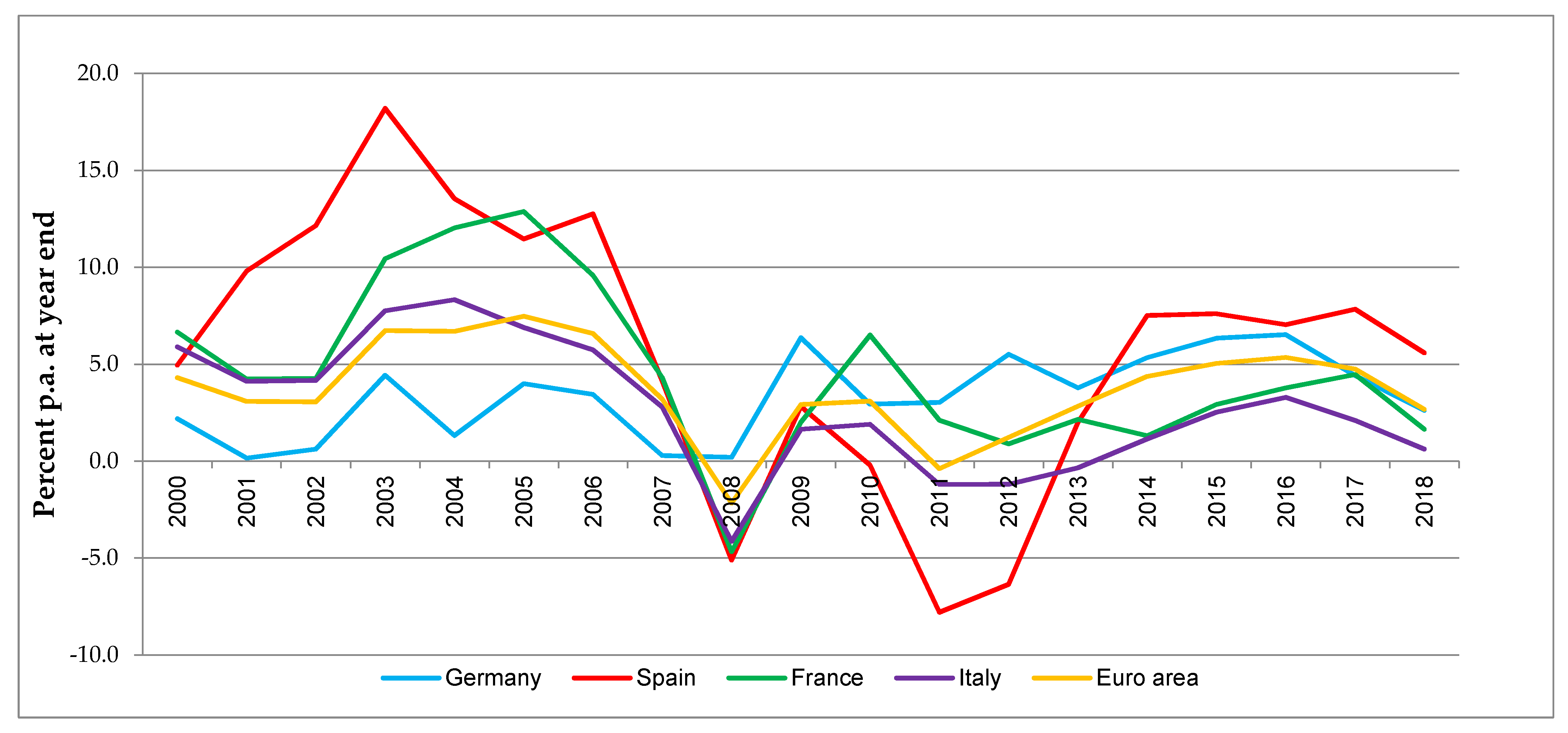
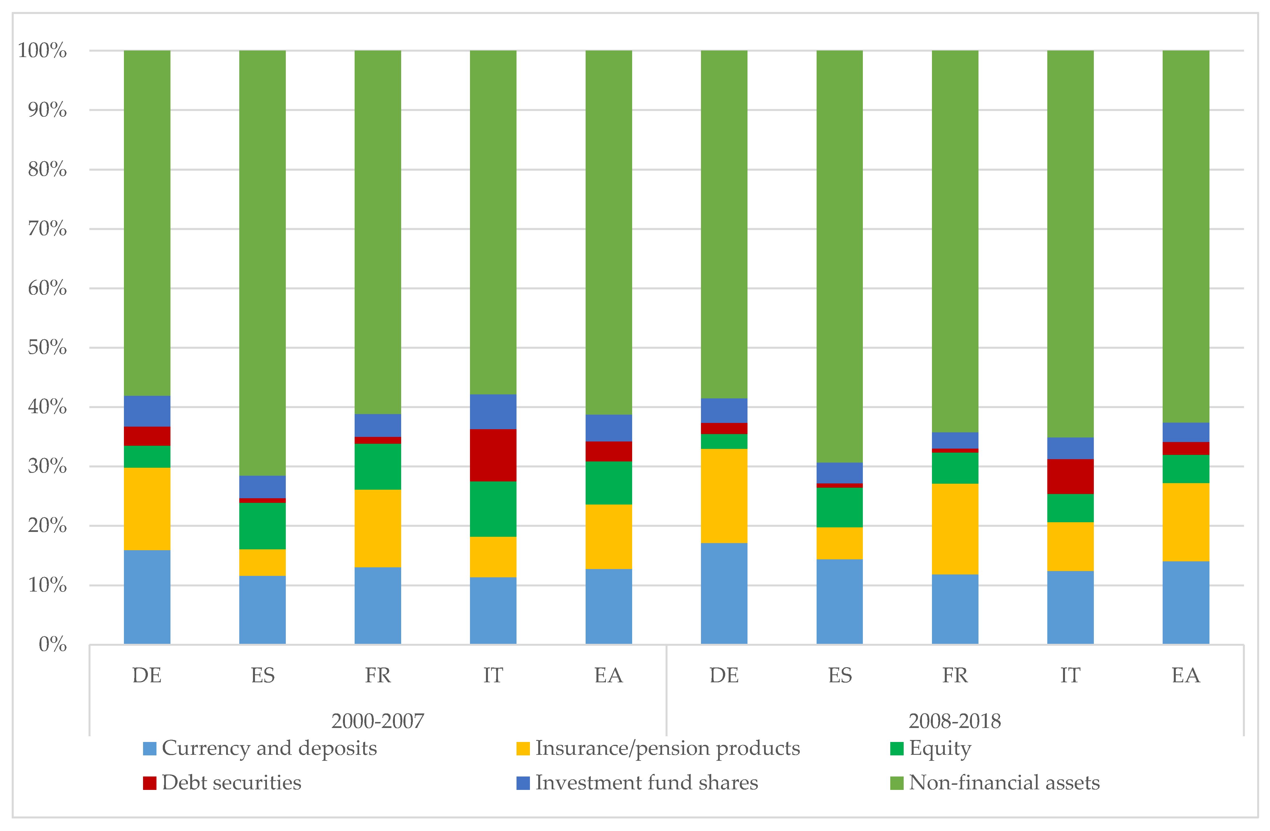
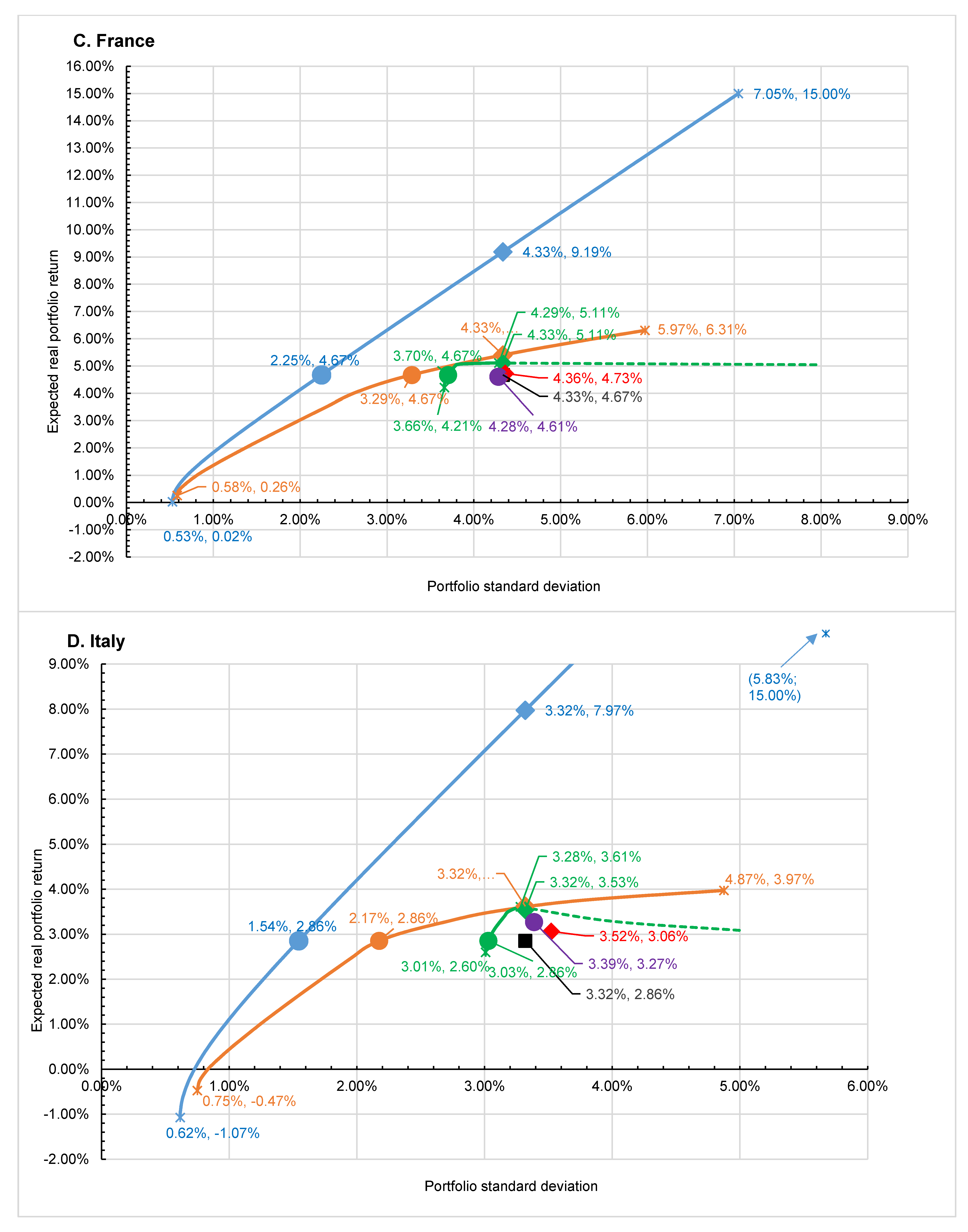
Table 1.
Descriptive statistics—real yields on total, financial and non-financial wealth.
| A. Germany | |||||||||
| Total Wealth | Financial Wealth | Non-Financial Wealth | |||||||
| 2000–2007 | 2008–2018 | 2000–2018 | 2000–2007 | 2008–2018 | 2000–2018 | 2000–2007 | 2008–2018 | 2000–2018 | |
| Mean | 2.06 | 4.28 | 3.34 | 2.02 | 1.77 | 1.87 | 2.06 | 6.05 | 4.37 |
| Median | 1.75 | 4.41 | 3.44 | 2.17 | 2.55 | 2.55 | 2.60 | 6.47 | 3.86 |
| Maximum | 4.43 | 6.52 | 6.52 | 5.61 | 5.81 | 5.81 | 3.86 | 9.37 | 9.37 |
| Minimum | 0.16 | 0.19 | 0.16 | −1.53 | −3.48 | −3.48 | −0.59 | 2.34 | −0.59 |
| Std. Dev. | 1.72 | 1.99 | 2.15 | 2.54 | 2.74 | 2.58 | 1.76 | 2.25 | 2.85 |
| Skewness | 0.23 | −0.60 | −0.08 | −0.07 | −0.64 | −0.46 | −0.45 | −0.26 | 0.04 |
| Kurtosis | 1.44 | 2.53 | 1.85 | 1.81 | 2.48 | 2.34 | 1.60 | 2.26 | 2.18 |
| Jarque–Bera | 0.88 | 0.76 | 1.07 | 0.48 | 0.88 | 1.00 | 0.92 | 0.37 | 0.54 |
| Probability | 0.64 | 0.68 | 0.59 | 0.79 | 0.64 | 0.61 | 0.63 | 0.83 | 0.76 |
| Observations | 8 | 11 | 19 | 8 | 11 | 19 | 8 | 11 | 19 |
| B. Spain | |||||||||
| Total Wealth | Financial Wealth | Non-Financial Wealth | |||||||
| 2000–2007 | 2008–2018 | 2000–2018 | 2000–2007 | 2008–2018 | 2000–2018 | 2000–2007 | 2008–2018 | 2000–2018 | |
| Mean | 10.87 | 1.90 | 5.68 | 1.62 | 1.44 | 1.51 | 14.55 | 2.28 | 7.45 |
| Median | 11.80 | 2.81 | 7.04 | 3.29 | 1.55 | 2.01 | 14.89 | 0.29 | 9.19 |
| Maximum | 18.20 | 7.84 | 18.20 | 7.44 | 11.71 | 11.71 | 22.64 | 10.78 | 22.64 |
| Minimum | 4.14 | −7.79 | −7.79 | −7.26 | −8.81 | −8.81 | 4.90 | −10.10 | −10.10 |
| Std. Dev. | 4.59 | 5.96 | 6.98 | 5.38 | 5.39 | 5.23 | 5.65 | 7.99 | 9.30 |
| Skewness | −0.15 | −0.53 | −0.40 | −0.48 | 0.03 | −0.18 | −0.36 | −0.35 | −0.42 |
| Kurtosis | 2.28 | 1.75 | 2.55 | 1.79 | 3.07 | 2.54 | 2.36 | 1.70 | 2.33 |
| Jarque–Bera | 0.20 | 1.23 | 0.66 | 0.80 | 0.00 | 0.27 | 0.32 | 1.00 | 0.90 |
| Probability | 0.90 | 0.54 | 0.72 | 0.67 | 1.00 | 0.87 | 0.85 | 0.61 | 0.64 |
| Observations | 8 | 11 | 19 | 8 | 11 | 19 | 8 | 11 | 19 |
| C. France | |||||||||
| Total Wealth | Financial Wealth | Non-Financial Wealth | |||||||
| 2000–2007 | 2008–2018 | 2000–2018 | 2000–2007 | 2008–2018 | 2000–2018 | 2000–2007 | 2008–2018 | 2000–2018 | |
| Mean | 8.05 | 2.10 | 4.61 | 2.10 | 1.99 | 2.03 | 12.00 | 2.17 | 6.31 |
| Median | 8.12 | 2.11 | 4.24 | 3.00 | 3.46 | 3.46 | 11.49 | 2.53 | 5.04 |
| Maximum | 12.87 | 6.50 | 12.87 | 7.48 | 8.44 | 8.44 | 16.64 | 8.49 | 16.64 |
| Minimum | 4.24 | −4.67 | −4.67 | −6.88 | −8.47 | −8.47 | 5.58 | −2.78 | −2.78 |
| Std. Dev. | 3.63 | 2.77 | 4.30 | 5.11 | 4.51 | 4.63 | 3.46 | 3.31 | 5.97 |
| Skewness | 0.09 | −1.04 | 0.25 | −0.72 | −1.07 | −0.90 | −0.42 | 0.27 | 0.20 |
| Kurtosis | 1.37 | 4.73 | 3.00 | 2.22 | 3.80 | 3.00 | 2.70 | 2.32 | 1.85 |
| Jarque–Bera | 0.90 | 3.33 | 0.20 | 0.90 | 2.38 | 2.54 | 0.27 | 0.34 | 1.18 |
| Probability | 0.64 | 0.19 | 0.91 | 0.64 | 0.30 | 0.28 | 0.87 | 0.84 | 0.55 |
| Observations | 8 | 11 | 19 | 8 | 11 | 19 | 8 | 11 | 19 |
| D. Italy | |||||||||
| Total Wealth | Financial Wealth | Non-Financial Wealth | |||||||
| 2000–2007 | 2008–2018 | 2000–2018 | 2000–2007 | 2008–2018 | 2000–2018 | 2000–2007 | 2008–2018 | 2000–2018 | |
| Mean | 5.71 | 0.58 | 2.74 | 1.44 | 1.02 | 1.20 | 8.91 | 0.38 | 3.97 |
| Median | 5.82 | 1.15 | 2.53 | 2.08 | 2.28 | 2.28 | 9.96 | 0.15 | 2.65 |
| Maximum | 8.33 | 3.29 | 8.33 | 5.88 | 6.37 | 6.37 | 11.28 | 4.24 | 11.28 |
| Minimum | 2.79 | −4.14 | −4.14 | −4.00 | −9.98 | −9.98 | 5.04 | −3.82 | −3.82 |
| Std. Dev. | 1.93 | 2.15 | 3.28 | 3.91 | 4.77 | 4.32 | 2.14 | 2.43 | 4.87 |
| Skewness | −0.10 | −0.87 | −0.09 | −0.26 | −1.16 | −0.95 | −0.74 | −0.15 | 0.11 |
| Kurtosis | 1.80 | 3.08 | 2.49 | 1.61 | 3.53 | 3.34 | 2.21 | 2.07 | 1.67 |
| Jarque–Bera | 0.49 | 1.40 | 0.23 | 0.73 | 2.58 | 2.95 | 0.94 | 0.44 | 1.43 |
| Probability | 0.78 | 0.50 | 0.89 | 0.69 | 0.28 | 0.23 | 0.63 | 0.80 | 0.49 |
| Observations | 8 | 11 | 19 | 8 | 11 | 19 | 8 | 11 | 19 |
| E. Euro Area | |||||||||
| Total Wealth | Financial Wealth | Non-Financial Wealth | |||||||
| 2000–2007 | 2008–2018 | 2000–2018 | 2000–2007 | 2008–2018 | 2000–2018 | 2000–2007 | 2008–2018 | 2000–2018 | |
| Mean | 5.14 | 2.70 | 3.73 | 1.81 | 1.65 | 1.72 | 7.35 | 3.37 | 5.05 |
| Median | 5.44 | 2.91 | 3.20 | 2.88 | 2.73 | 2.73 | 7.70 | 3.53 | 6.24 |
| Maximum | 7.48 | 5.35 | 7.48 | 6.43 | 7.45 | 7.45 | 8.44 | 7.07 | 8.44 |
| Minimum | 3.05 | −2.17 | −2.17 | −5.19 | −7.75 | −7.75 | 4.07 | −0.33 | −0.33 |
| Std. Dev. | 1.91 | 2.35 | 2.45 | 4.15 | 4.17 | 4.04 | 1.40 | 2.81 | 3.04 |
| Skewness | −0.05 | −0.84 | −0.61 | −0.61 | −1.01 | −0.85 | −1.84 | 0.00 | −0.59 |
| Kurtosis | 1.20 | 2.76 | 3.20 | 2.00 | 3.46 | 2.90 | 5.07 | 1.33 | 1.83 |
| Jarque–Bera | 1.08 | 1.31 | 1.19 | 0.83 | 1.96 | 2.29 | 5.93 | 1.27 | 2.18 |
| Probability | 0.58 | 0.52 | 0.55 | 0.66 | 0.38 | 0.32 | 0.05 | 0.53 | 0.34 |
| Observations | 8 | 11 | 19 | 8 | 11 | 19 | 8 | 11 | 19 |
Notes: 1. All statics either quoted in or based on percentages. 2. The respective national real returns on financial wealth were calculated as weighted real returns on all national financial assets. Consequently, since real national returns on non-financial and financial wealth have not been weighted with respect to total national assets, they do not add up to the respective national real returns on total wealth. 3. Jarque–Bera test statistic: H0: normal distribution. H1: non-normal distribution. A small probability leads to a rejection of H0. Source: authors’ calculations based on ECB, Eurostat, OECD, Thomson Reuters.
Table 2.
Descriptive statistics—real yields on individual assets.
| A. Germany | ||||||||||||||||||
| Currency and deposits | Debt securities | Equity | Investment fund shares | Insurance/pension products | Non-financial assets | |||||||||||||
| 2000–2007 | 2008–2018 | 2000–2018 | 2000–2007 | 2008–2018 | 2000–2018 | 2000–2007 | 2008–2018 | 2000–2018 | 2000–2007 | 2008–2018 | 2000–2018 | 2000–2007 | 2008–2018 | 2000–2018 | 2000–2007 | 2008–2018 | 2000–2018 | |
| Mean | 0.36 | −0.49 | −0.13 | 3.22 | 3.12 | 3.16 | 2.55 | 4.57 | 3.72 | 3.37 | 4.86 | 4.23 | 3.15 | 2.59 | 2.83 | 2.06 | 6.05 | 4.37 |
| Median | 0.25 | −0.27 | 0.02 | 3.34 | 3.07 | 3.12 | 9.69 | 9.54 | 9.54 | 2.61 | 6.50 | 6.50 | 2.91 | 2.59 | 2.59 | 2.60 | 6.47 | 3.86 |
| Maximum | 0.96 | 1.15 | 1.15 | 7.80 | 10.17 | 10.17 | 28.51 | 23.49 | 28.51 | 13.87 | 18.19 | 18.19 | 6.03 | 4.93 | 6.03 | 3.86 | 9.37 | 9.37 |
| Minimum | −0.17 | −1.71 | −1.71 | −2.03 | −2.09 | −2.09 | 40.69 | 42.73 | 42.73 | −7.95 | 18.82 | 18.82 | 1.61 | 0.47 | 0.47 | −0.59 | 2.34 | −0.59 |
| Std. Dev. | 0.41 | 0.85 | 0.81 | 3.27 | 4.10 | 3.67 | 23.67 | 20.46 | 21.25 | 8.94 | 10.48 | 9.63 | 1.42 | 1.27 | 1.32 | 1.76 | 2.25 | 2.85 |
| Skewness | 0.34 | 0.31 | −0.40 | −0.35 | 0.48 | 0.26 | −0.68 | −1.18 | −0.94 | −0.01 | −1.02 | −0.68 | 0.98 | 0.06 | 0.54 | −0.45 | −0.26 | 0.04 |
| Kurtosis | 1.77 | 2.33 | 2.34 | 2.12 | 1.89 | 2.02 | 2.31 | 3.54 | 2.90 | 1.27 | 3.38 | 2.71 | 3.10 | 2.52 | 3.30 | 1.60 | 2.26 | 2.18 |
| Jarque–Bera | 0.65 | 0.38 | 0.85 | 0.42 | 0.99 | 0.98 | 0.77 | 2.68 | 2.82 | 1.00 | 1.96 | 1.52 | 1.28 | 0.11 | 1.00 | 0.92 | 0.37 | 0.54 |
| Probability | 0.72 | 0.83 | 0.65 | 0.81 | 0.61 | 0.61 | 0.68 | 0.26 | 0.24 | 0.61 | 0.38 | 0.47 | 0.53 | 0.95 | 0.61 | 0.63 | 0.83 | 0.76 |
| Observations | 8 | 11 | 19 | 8 | 11 | 19 | 8 | 11 | 19 | 8 | 11 | 19 | 8 | 11 | 19 | 8 | 11 | 19 |
| B. Spain | ||||||||||||||||||
| Currency and deposits | Debt securities | Equity | Investment fund shares | Insurance/pension products | Non-financial assets | |||||||||||||
| 2000–2007 | 2008–2018 | 2000–2018 | 2000–2007 | 2008–2018 | 2000–2018 | 2000–2007 | 2008–2018 | 2000–2018 | 2000–2007 | 2008–2018 | 2000–2018 | 2000–2007 | 2008–2018 | 2000–2018 | 2000–2007 | 2008–2018 | 2000–2018 | |
| Mean | −2.18 | −0.37 | −1.13 | 1.90 | 3.37 | 2.75 | 4.59 | 1.45 | 2.77 | 0.77 | 2.39 | 1.71 | 3.93 | 4.98 | 4.54 | 14.55 | 2.28 | 7.45 |
| Median | −2.20 | −0.56 | −1.40 | 2.74 | 1.92 | 2.17 | 10.78 | 3.19 | 4.25 | 0.05 | 2.19 | 2.02 | 4.33 | 4.45 | 4.45 | 14.89 | 0.29 | 9.19 |
| Maximum | −0.67 | 1.61 | 1.61 | 6.10 | 10.80 | 10.80 | 25.36 | 39.55 | 39.55 | 3.65 | 8.06 | 8.06 | 5.67 | 7.82 | 7.82 | 22.64 | 10.78 | 22.64 |
| Minimum | −3.10 | −1.89 | −3.10 | −3.93 | −1.46 | −3.93 | −30.97 | −39.51 | −39.51 | −2.69 | −3.26 | −3.26 | 1.22 | 3.19 | 1.22 | 4.90 | −10.10 | −10.10 |
| Std. Dev. | 0.73 | 1.20 | 1.36 | 3.23 | 4.21 | 3.81 | 20.30 | 20.70 | 20.02 | 2.22 | 3.71 | 3.20 | 1.55 | 1.68 | 1.67 | 5.65 | 7.99 | 9.30 |
| Skewness | 0.89 | 0.32 | 0.55 | −0.61 | 0.41 | 0.31 | −0.58 | −0.08 | −0.29 | 0.05 | 0.16 | 0.46 | −0.66 | 0.42 | 0.10 | −0.36 | −0.35 | −0.42 |
| Kurtosis | 3.55 | 1.72 | 2.28 | 2.42 | 1.80 | 2.43 | 2.04 | 3.15 | 2.66 | 1.89 | 1.93 | 2.44 | 2.20 | 1.65 | 2.59 | 2.36 | 1.70 | 2.33 |
| Jarque–Bera | 1.17 | 0.94 | 1.37 | 0.60 | 0.96 | 0.56 | 0.76 | 0.02 | 0.35 | 0.42 | 0.58 | 0.91 | 0.80 | 1.15 | 0.17 | 0.32 | 1.00 | 0.90 |
| Probability | 0.56 | 0.62 | 0.50 | 0.74 | 0.62 | 0.76 | 0.68 | 0.99 | 0.84 | 0.81 | 0.75 | 0.64 | 0.67 | 0.56 | 0.92 | 0.85 | 0.61 | 0.64 |
| Observations | 8 | 11 | 19 | 8 | 11 | 19 | 8 | 11 | 19 | 8 | 11 | 19 | 8 | 11 | 19 | 8 | 11 | 19 |
| C. France | ||||||||||||||||||
| Currency and deposits | Debt securities | Equity | Investment fund shares | Insurance/pension products | Non-financial assets | |||||||||||||
| 2000–2007 | 2008–2018 | 2000–2018 | 2000–2007 | 2008–2018 | 2000–2018 | 2000–2007 | 2008–2018 | 2000–2018 | 2000–2007 | 2008–2018 | 2000–2018 | 2000–2007 | 2008–2018 | 2000–2018 | 2000–2007 | 2008–2018 | 2000–2018 | |
| Mean | 0.22 | 0.08 | 0.14 | 3.05 | 3.03 | 3.04 | 1.62 | 4.01 | 3.00 | 1.51 | 1.57 | 1.55 | 4.04 | 2.57 | 3.19 | 12.00 | 2.17 | 6.31 |
| Median | 0.23 | −0.13 | 0.18 | 3.60 | 2.39 | 2.44 | 4.36 | 9.19 | 7.80 | 2.00 | 2.63 | 2.63 | 5.90 | 3.28 | 3.98 | 11.49 | 2.53 | 5.04 |
| Maximum | 0.72 | 1.40 | 1.40 | 7.34 | 10.96 | 10.96 | 25.03 | 28.77 | 28.77 | 4.91 | 8.83 | 8.83 | 7.40 | 7.29 | 7.40 | 16.64 | 8.49 | 16.64 |
| Minimum | −0.15 | −1.24 | −1.24 | −2.26 | −1.93 | −2.26 | −34.02 | −41.37 | −41.37 | −3.85 | −9.12 | −9.12 | −2.94 | −5.65 | −5.65 | 5.58 | −2.78 | −2.78 |
| Std. Dev. | 0.27 | 0.76 | 0.60 | 3.12 | 4.18 | 3.67 | 19.66 | 19.48 | 19.04 | 3.48 | 4.73 | 4.14 | 3.78 | 3.35 | 3.51 | 3.46 | 3.31 | 5.97 |
| Skewness | 0.44 | 0.11 | −0.11 | −0.41 | 0.77 | 0.52 | −0.70 | −1.10 | −0.93 | −0.29 | −0.85 | −0.75 | −1.03 | −1.31 | −1.03 | −0.42 | 0.27 | 0.20 |
| Kurtosis | 2.74 | 2.28 | 3.29 | 2.20 | 2.25 | 2.41 | 2.39 | 3.72 | 3.12 | 1.49 | 3.62 | 3.54 | 2.45 | 4.57 | 3.42 | 2.70 | 2.32 | 1.85 |
| Jarque–Bera | 0.28 | 0.26 | 0.11 | 0.44 | 1.35 | 1.13 | 0.77 | 2.47 | 2.74 | 0.87 | 1.51 | 2.01 | 1.53 | 4.29 | 3.53 | 0.27 | 0.34 | 1.18 |
| Probability | 0.87 | 0.88 | 0.95 | 0.80 | 0.51 | 0.57 | 0.68 | 0.29 | 0.25 | 0.65 | 0.47 | 0.37 | 0.47 | 0.12 | 0.17 | 0.87 | 0.84 | 0.55 |
| Observations | 8 | 11 | 19 | 8 | 11 | 19 | 8 | 11 | 19 | 8 | 11 | 19 | 8 | 11 | 19 | 8 | 11 | 19 |
| D. Italy | ||||||||||||||||||
| Currency and deposits | Debt securities | Equity | Investment fund shares | Insurance/pension products | Non-financial assets | |||||||||||||
| 2000–2007 | 2008–2018 | 2000–2018 | 2000–2007 | 2008–2018 | 2000–2018 | 2000–2007 | 2008–2018 | 2000–2018 | 2000–2007 | 2008–2018 | 2000–2018 | 2000–2007 | 2008–2018 | 2000–2018 | 2000–2007 | 2008–2018 | 2000–2018 | |
| Mean | −1.11 | −0.68 | −0.86 | 2.81 | 3.10 | 2.98 | 1.41 | −0.10 | 0.54 | 2.37 | 2.84 | 2.64 | 2.60 | 1.89 | 2.19 | 8.91 | 0.38 | 3.97 |
| Median | −1.15 | −0.79 | −0.93 | 3.61 | 2.13 | 2.23 | 6.05 | 7.59 | 7.59 | 1.97 | 3.71 | 2.10 | 2.72 | 3.23 | 2.75 | 9.96 | 0.15 | 2.65 |
| Maximum | −0.35 | 0.53 | 0.53 | 6.82 | 14.34 | 14.34 | 17.82 | 23.46 | 23.46 | 6.34 | 9.88 | 9.88 | 3.98 | 5.06 | 5.06 | 11.28 | 4.24 | 11.28 |
| Minimum | −1.68 | −2.12 | −2.12 | −2.68 | −5.29 | −5.29 | −25.58 | −46.97 | −46.97 | −1.58 | −5.81 | −5.81 | 0.60 | −4.38 | −4.38 | 5.04 | −3.82 | −3.82 |
| Std. Dev. | 0.42 | 0.98 | 0.81 | 3.26 | 5.75 | 4.74 | 17.28 | 19.74 | 18.25 | 3.01 | 5.04 | 4.20 | 1.11 | 2.75 | 2.19 | 2.14 | 2.43 | 4.87 |
| Skewness | 0.39 | −0.18 | 0.31 | −0.46 | 0.67 | 0.64 | −0.56 | −1.20 | −1.02 | 0.09 | −0.22 | −0.11 | −0.61 | −1.11 | −1.53 | −0.74 | −0.15 | 0.11 |
| Kurtosis | 2.53 | 1.69 | 2.18 | 2.03 | 2.71 | 3.36 | 1.78 | 3.89 | 3.44 | 1.55 | 2.03 | 2.34 | 2.39 | 3.40 | 5.32 | 2.21 | 2.07 | 1.67 |
| Jarque–Bera | 0.28 | 0.85 | 0.84 | 0.60 | 0.87 | 1.40 | 0.91 | 2.99 | 3.44 | 0.71 | 0.52 | 0.38 | 0.62 | 2.34 | 11.67 | 0.94 | 0.44 | 1.43 |
| Probability | 0.87 | 0.66 | 0.66 | 0.74 | 0.65 | 0.50 | 0.63 | 0.22 | 0.18 | 0.70 | 0.77 | 0.83 | 0.73 | 0.31 | 0.00 | 0.63 | 0.80 | 0.49 |
| Observations | 8 | 11 | 19 | 8 | 11 | 19 | 8 | 11 | 19 | 8 | 11 | 19 | 8 | 11 | 19 | 8 | 11 | 19 |
| E. Euro area | ||||||||||||||||||
| Currency and deposits | Debt securities | Equity | Investment fund shares | Insurance/pension products | Non-financial assets | |||||||||||||
| 2000–2007 | 2008–2018 | 2000–2018 | 2000–2007 | 2008–2018 | 2000–2018 | 2000–2007 | 2008–2018 | 2000–2018 | 2000–2007 | 2008–2018 | 2000–2018 | 2000–2007 | 2008–2018 | 2000–2018 | 2000–2007 | 2008–2018 | 2000–2018 | |
| Mean | −0.30 | −0.37 | −0.34 | 2.91 | 3.10 | 3.02 | 1.90 | 2.91 | 2.49 | 2.38 | 3.22 | 2.87 | 3.44 | 2.63 | 2.97 | 7.35 | 3.37 | 5.05 |
| Median | −0.37 | −0.39 | −0.39 | 3.77 | 2.36 | 2.63 | 7.70 | 6.19 | 6.19 | 2.00 | 4.41 | 4.06 | 3.86 | 3.45 | 3.47 | 7.70 | 3.53 | 6.24 |
| Maximum | 0.15 | 1.03 | 1.03 | 7.10 | 12.71 | 12.71 | 23.61 | 28.02 | 28.02 | 7.78 | 11.99 | 11.99 | 5.47 | 6.01 | 6.01 | 8.44 | 7.07 | 8.44 |
| Minimum | −0.63 | −1.35 | −1.35 | −2.55 | −3.36 | −3.36 | −34.68 | −45.34 | −45.34 | −3.88 | −11.08 | −11.08 | 1.02 | −2.28 | −2.28 | 4.07 | −0.33 | −0.33 |
| Std. Dev. | 0.26 | 0.81 | 0.63 | 3.23 | 4.99 | 4.23 | 20.22 | 20.58 | 19.86 | 4.92 | 6.68 | 5.86 | 1.35 | 2.18 | 1.88 | 1.40 | 2.81 | 3.04 |
| Skewness | 0.75 | 0.33 | 0.28 | −0.48 | 0.71 | 0.59 | −0.74 | −1.14 | −0.98 | 0.02 | −0.80 | −0.58 | −0.42 | −0.86 | −1.06 | −1.84 | 0.00 | −0.59 |
| Kurtosis | 2.40 | 1.76 | 2.61 | 2.12 | 2.50 | 2.90 | 2.28 | 3.78 | 3.18 | 1.29 | 2.94 | 2.74 | 2.65 | 3.59 | 4.49 | 5.07 | 1.33 | 1.83 |
| Jarque–Bera | 0.86 | 0.90 | 0.37 | 0.56 | 1.05 | 1.10 | 0.91 | 2.65 | 3.05 | 0.98 | 1.17 | 1.10 | 0.28 | 1.52 | 5.32 | 5.93 | 1.27 | 2.18 |
| Probability | 0.65 | 0.64 | 0.83 | 0.76 | 0.59 | 0.58 | 0.64 | 0.27 | 0.22 | 0.61 | 0.56 | 0.58 | 0.87 | 0.47 | 0.07 | 0.05 | 0.53 | 0.34 |
| Observations | 8 | 11 | 19 | 8 | 11 | 19 | 8 | 11 | 19 | 8 | 11 | 19 | 8 | 11 | 19 | 8 | 11 | 19 |
Notes: 1. All statistics either quoted in or based on percentages. 2. Jarque–Bera test statistic: H0: normal distribution; H1: non-normal distribution. A small probability leads to a rejection of H0. Source: authors’ calculations based on ECB, Eurostat, OECD, Thomson Reuters.
Table 3.
Variance-covariance matrices and correlations.
| A. Germany | ||||||
| Covariance Correlation | Currency and deposits | Debt securities | Equity | Investment fund shares | Insurance/pension products | Non-financial assets |
| Currency and deposits | 0.66 | |||||
| 1.00 | ||||||
| Debt securities | 1.09 | 13.50 | ||||
| 0.37 | 1.00 | |||||
| Equity | 0.77 | −2.10 | 451.49 | |||
| 0.04 | −0.03 | 1.00 | ||||
| Investment fund shares | 1.07 | 9.74 | 183.74 | 92.64 | ||
| 0.14 | 0.28 | 0.90 | 1.00 | |||
| Insurance products | 0.73 | 2.32 | 4.88 | 4.23 | 1.75 | |
| 0.68 | 0.48 | 0.17 | 0.33 | 1.00 | ||
| Non-financial assets | −0.68 | 0.28 | 14.32 | 8.15 | 0.20 | 8.11 |
| −0.29 | 0.03 | 0.24 | 0.30 | 0.05 | 1.00 | |
| B. Spain | ||||||
| Covariance Correlation | Currency and deposits | Debt securities | Equity | Investment fund shares | Insurance/pension products | Non-financial assets |
| Currency and deposits | 1.84 | |||||
| 1.00 | ||||||
| Debt securities | 1.83 | 14.48 | ||||
| 0.35 | 1.00 | |||||
| Equity | 9.69 | 10.57 | 400.82 | |||
| 0.36 | 0.14 | 1.00 | ||||
| Investment fund shares | 2.38 | 8.02 | 37.73 | 10.23 | ||
| 0.55 | 0.66 | 0.59 | 1.00 | |||
| Insurance products | 1.42 | 3.09 | −1.24 | 2.00 | 2.78 | |
| 0.63 | 0.49 | −0.04 | 0.37 | 1.00 | ||
| Non-financial assets | −5.16 | −5.62 | 28.64 | −2.67 | −1.30 | 86.57 |
| −0.41 | −0.16 | 0.15 | −0.09 | −0.08 | 1.00 | |
| C. France | ||||||
| Covariance Correlation | Currency and deposits | Debt securities | Equity | Investment fund shares | Insurance/pension products | Non-financial assets |
| Currency and deposits | 0.35 | |||||
| 1.00 | ||||||
| Debt securities | 0.53 | 13.47 | ||||
| 0.24 | 1.00 | |||||
| Equity | 4.29 | 2.26 | 362.71 | |||
| 0.38 | 0.03 | 1.00 | ||||
| Investment fund shares | 0.95 | 3.56 | 72.38 | 17.14 | ||
| 0.39 | 0.23 | 0.92 | 1.00 | |||
| Insurance products | 0.91 | 0.16 | 59.83 | 12.88 | 12.34 | |
| 0.43 | 0.01 | 0.89 | 0.89 | 1.00 | ||
| Non-financial assets | −0.35 | −2.35 | 5.17 | 3.78 | 6.31 | 35.65 |
| −0.10 | −0.11 | 0.05 | 0.15 | 0.30 | 1.00 | |
| D. Italy | ||||||
| Covariance Correlation | Currency and deposits | Debt securities | Equity | Investment fund shares | Insurance/pension products | Non-financial assets |
| Currency and deposits | 0.66 | |||||
| 1.00 | ||||||
| Debt securities | 0.11 | 22.51 | ||||
| 0.03 | 1.00 | |||||
| Equity | 6.09 | 16.68 | 333.20 | |||
| 0.41 | 0.19 | 1.00 | ||||
| Investment fund shares | 1.04 | 13.14 | 59.06 | 17.68 | ||
| 0.30 | 0.66 | 0.77 | 1.00 | |||
| Insurance products | 1.15 | 2.39 | 31.99 | 6.52 | 4.82 | |
| 0.64 | 0.23 | 0.80 | 0.71 | 1.00 | ||
| Non-financial assets | −0.71 | −3.81 | −2.11 | −2.17 | 1.95 | 23.76 |
| −0.18 | −0.16 | −0.02 | −0.11 | 0.18 | 1.00 | |
| E. Euro area | ||||||
| Covariance Correlation | Currency and deposits | Debt securities | Equity | Investment fund shares | Insurance/pension products | Non-financial assets |
| Currency and deposits | 0.40 | |||||
| 1.00 | ||||||
| Debt securities | 0.70 | 17.91 | ||||
| 0.26 | 1.00 | |||||
| Equity | 3.82 | 8.79 | 394.60 | |||
| 0.31 | 0.10 | 1.00 | ||||
| Investment fund shares | 1.32 | 10.45 | 103.06 | 34.35 | ||
| 0.36 | 0.42 | 0.89 | 1.00 | |||
| Insurance products | 0.71 | 1.52 | 29.27 | 8.75 | 3.52 | |
| 0.60 | 0.19 | 0.79 | 0.80 | 1.00 | ||
| Non-financial assets | 0.14 | −1.84 | 0.37 | 0.12 | 1.37 | 9.23 |
| 0.07 | −0.14 | 0.01 | 0.01 | 0.24 | 1.00 |
Notes: 1. Sample: 2000 to 2018; 2. Degrees-of-freedom-corrected covariances; covariances in squared percentage returns. Source: authors’ calculations.
Table 4.
Minimum variance and maximum expected real return portfolios.
| A. Germany | ||||||||||
| Portfolio 2018 | Optimal mean-variance portfolios | |||||||||
| Model 1 | Model 2 | Model 3 | ||||||||
| Minimum variance | Maximum expected real return | Minimum variance | Maximum expected real return | Minimum variance | Maximum expected real return | |||||
| Asset categories | ||||||||||
| Expected real return | standard deviation | Coefficient of variation | Portfolio shares | |||||||
| Currency and deposits | −0.13 | 0.81 | −6.15 | 17.74 | 101.00 | −228.30 | 86.77 | 0.00 | 41.96 | 0.00 |
| Insurance/pension products | 2.83 | 1.32 | 0.47 | 16.03 | −13.54 | 292.46 | 0.00 | 0.00 | 0.00 | 0.00 |
| Equity | 3.72 | 21.25 | 5.71 | 2.66 | 0.57 | 6.02 | 0.00 | 0.00 | 0.00 | 0.00 |
| Debt securities | 3.16 | 3.67 | 1.16 | 1.07 | −1.15 | 10.08 | 0.00 | 0.00 | 0.00 | 0.00 |
| Investment fund shares | 4.23 | 9.63 | 2.27 | 4.46 | −2.47 | −22.61 | 0.00 | 0.00 | 0.00 | 41.96 |
| Non-financial assets | 4.37 | 2.85 | 0.65 | 58.04 | 15.59 | 42.35 | 13.23 | 100.00 | 58.04 | 58.04 |
| Portfolio performance | ||||||||||
| Expected real portfolio return | 3.29 | 0.05 | 10.00 | 0.46 | 4.37 | 2.48 | 4.31 | |||
| Portfolio standard deviation | 2.17 | 0.65 | 3.18 | 0.69 | 2.84 | 1.59 | 4.80 | |||
| Coefficient of variation | 0.66 | 14.17 | 0.32 | 1.50 | 0.65 | 0.64 | 1.11 | |||
| B. Spain | ||||||||||
| Portfolio 2018 | Optimal mean-variance portfolios | |||||||||
| Model 1 | Model 2 | Model 3 | ||||||||
| Minimum variance | Maximum expected real return | Minimum variance | Maximum expected real return | Minimum variance | Maximum expected real return | |||||
| Asset categories | ||||||||||
| Expected real return | standard deviation | Coefficient of variation | Portfolio shares | |||||||
| Currency and deposits | −1.13 | 1.36 | −1.20 | 14.55 | 110.80 | −547.57 | 85.99 | 0.00 | 30.21 | 0.00 |
| Insurance/pension products | 4.54 | 1.67 | 0.37 | 5.90 | −19.54 | 673.50 | 7.23 | 0.00 | 0.00 | 32.72 |
| Equity | 2.77 | 20.02 | 7.22 | 6.94 | −3.17 | 16.52 | 0.00 | 0.00 | 0.00 | 0.00 |
| Debt securities | 2.75 | 3.81 | 1.38 | 0.28 | 3.34 | −62.71 | 0.00 | 0.00 | 2.51 | 0.00 |
| Investment fund shares | 1.71 | 3.20 | 1.87 | 5.05 | −0.22 | 35.25 | 0.00 | 0.00 | 0.00 | 0.00 |
| Non-financial assets | 7.45 | 9.30 | 1.25 | 67.28 | 8.79 | −14.99 | 6.78 | 100.00 | 67.28 | 67.28 |
| Portfolio performance | ||||||||||
| Expected real portfolio return | 5.40 | −1.49 | 35.00 | −0.14 | 7.45 | 4.74 | 6.45 | |||
| Portfolio standard deviation | 6.56 | 1.03 | 7.30 | 1.16 | 9.30 | 6.09 | 6.23 | |||
| Coefficient of variation | 1.22 | −0.69 | 0.21 | −8.17 | 1.25 | 1.29 | 0.97 | |||
| C. France | ||||||||||
| Portfolio 2018 | Optimal mean-variance portfolios | |||||||||
| Model 1 | Model 2 | Model 3 | ||||||||
| Minimum variance | Maximum expected real return | Minimum variance | Maximum expected real return | Minimum variance | Maximum expected real return | |||||
| Asset categories | ||||||||||
| Expected real return | standard deviation | Coefficient of variation | Portfolio shares | |||||||
| Currency and deposits | 0.14 | 0.60 | 4.34 | 12.82 | 101.18 | −274.42 | 98.08 | 0.00 | 29.09 | 0.00 |
| Insurance/pension products | 3.19 | 3.51 | 1.10 | 16.50 | −7.07 | 451.34 | 0.00 | 0.00 | 0.00 | 38.23 |
| Equity | 3.00 | 19.04 | 6.35 | 6.32 | −1.79 | −29.81 | 0.00 | 0.00 | 0.00 | 0.00 |
| Debt securities | 3.04 | 3.67 | 1.21 | 0.38 | −3.58 | 140.63 | 0.00 | 0.00 | 9.14 | 0.00 |
| Investment fund shares | 1.55 | 4.14 | 2.67 | 2.20 | 9.19 | −198.67 | 0.00 | 0.00 | 0.00 | 0.00 |
| Non-financial assets | 6.31 | 5.97 | 0.95 | 61.77 | 2.08 | 10.93 | 1.92 | 100.00 | 61.77 | 61.77 |
| Portfolio performance | ||||||||||
| Expected real portfolio return | 4.67 | 0.02 | 15.00 | 0.26 | 6.31 | 4.21 | 5.11 | |||
| Portfolio standard deviation | 4.33 | 0.53 | 7.05 | 0.58 | 5.97 | 3.66 | 4.29 | |||
| Coefficient of variation | 0.93 | 21.46 | 0.47 | 2.28 | 0.95 | 0.87 | 0.84 | |||
| D. Italy | ||||||||||
| Portfolio 2018 | Optimal mean-variance portfolios | |||||||||
| Model 1 | Model 2 | Model 3 | ||||||||
| Minimum variance | Maximum expected real return | Minimum variance | Maximum expected real return | Minimum variance | Maximum expected real return | |||||
| Asset categories | ||||||||||
| Expected real return | standard deviation | Coefficient of variation | Portfolio shares | |||||||
| Currency and deposits | −0.86 | 0.81 | −0.94 | 14.00 | 114.12 | −392.82 | 91.41 | 0.00 | 27.39 | 0.00 |
| Insurance/pension products | 2.19 | 2.19 | 1.00 | 10.08 | −33.04 | 507.72 | 0.00 | 0.00 | 0.00 | 0.00 |
| Equity | 0.54 | 18.25 | 34.02 | 4.88 | −0.59 | −48.76 | 0.00 | 0.00 | 0.00 | 0.00 |
| Debt securities | 2.98 | 4.74 | 1.59 | 2.95 | 0.56 | −6.19 | 3.01 | 0.00 | 9.42 | 36.82 |
| Investment fund shares | 2.64 | 4.20 | 1.59 | 4.90 | 10.25 | 48.39 | 0.00 | 0.00 | 0.00 | 0.00 |
| Non-financial assets | 3.97 | 4.87 | 1.23 | 63.18 | 8.69 | −8.34 | 5.58 | 100.00 | 63.18 | 63.18 |
| Portfolio performance | ||||||||||
| Expected real portfolio return | 2.86 | −1.07 | 15.00 | −0.47 | 3.97 | 2.56 | 3.61 | |||
| Portfolio standard deviation | 3.32 | 0.62 | 5.83 | 0.75 | 4.87 | 3.01 | 3.28 | |||
| Coefficient of variation | 1.16 | −0.57 | 0.39 | −1.58 | 1.23 | 1.18 | 0.91 | |||
| E. Euro area | ||||||||||
| Portfolio 2018 | Optimal mean-variance portfolios | |||||||||
| Model 1 | Model 2 | Model 3 | ||||||||
| Minimum variance | Maximum expected real return | Minimum variance | Maximum expected real return | Minimum variance | Maximum expected real return | |||||
| Asset categories | ||||||||||
| Expected real return | standard deviation | Coefficient of variation | Portfolio shares | |||||||
| Currency and deposits | −0.34 | 0.63 | −1.85 | 15.03 | 114.08 | −194.23 | 97.28 | 0.00 | 33.22 | 0.00 |
| Insurance/pension products | 2.97 | 1.88 | 0.63 | 14.68 | −19.06 | 283.55 | 0.00 | 0.00 | 0.00 | 0.00 |
| Equity | 2.49 | 19.86 | 7.99 | 5.05 | −0.65 | −10.82 | 0.00 | 0.00 | 0.00 | 0.00 |
| Debt securities | 3.02 | 4.23 | 1.40 | 1.03 | −2.70 | 29.19 | 0.00 | 0.00 | 6.36 | 39.57 |
| Investment fund shares | 2.87 | 5.86 | 2.04 | 3.79 | 4.19 | −31.50 | 0.00 | 0.00 | 0.00 | 0.00 |
| Non-financial assets | 5.05 | 3.04 | 0.60 | 60.43 | 4.13 | 23.82 | 2.72 | 100.00 | 60.43 | 60.43 |
| Portfolio performance | ||||||||||
| Expected real portfolio return | 3.70 | −0.72 | 10.00 | −0.19 | 5.05 | 3.13 | 4.24 | |||
| Portfolio standard deviation | 2.42 | 0.58 | 3.06 | 0.62 | 3.04 | 1.85 | 2.30 | |||
| Coefficient of variation | 0.65 | −0.80 | 0.31 | −3.23 | 0.60 | 0.59 | 0.54 | |||
Notes: 1. All numbers, except for the Coefficient of variation being dimensionless, in percentages; 2. Time range for computation of individual assets’ expected real returns and standard deviations: 2000–2018. Individual assets’ expected real returns are computed as arithmetic averages. 3. Coefficient of variation computed as the ratio of the standard deviation to expected real return. Source: authors’ calculations.
Table 5.
Mean-variance “ceteris paribus portfolios” and heuristic portfolios.
| A. Germany | ||||||||||||
| Portfolio 2018 | Mean-variance “ceteris paribus” portfolios | Heuristic portfolios | ||||||||||
| Model 1 | Model 2 | Model 3 | ||||||||||
| (1a) | (1b) | (2a) | (2b) | (3a) | (3b) | |||||||
| Standard deviation 2018 + expected real return maximized | Expected real return 2018 + standard deviation minimized | Standard deviation 2018 + expected real return maximized | Expected real return 2018 + standard deviation minimized | Standard deviation 2018 + expected real return maximized | Expected real return 2018 + standard deviation minimized | 1/n portfolio | Opportunity portfolio | |||||
| Asset categories | ||||||||||||
| Expected real return | Standard deviation | Coefficient of variation | Portfolio shares | |||||||||
| Currency and deposits | −0.13 | 0.81 | −6.15 | 17.74 | −117.76 | −6.27 | 0.00 | 0.00 | 0.00 | 14.69 | 8.39 | 4.20 |
| Insurance/pension products | 2.83 | 1.32 | 0.47 | 16.03 | 189.74 | 86.14 | 17.67 | 70.04 | 16.08 | 27.27 | 8.39 | 4.20 |
| Equity | 3.72 | 21.25 | 5.71 | 2.66 | 4.19 | 2.35 | 0.00 | 0.00 | 0.00 | 0.00 | 8.39 | 4.20 |
| Debt securities | 3.16 | 3.67 | 1.16 | 1.07 | 6.31 | 2.51 | 8.95 | 0.00 | 20.36 | 0.00 | 8.39 | 4.20 |
| Investment fund shares | 4.23 | 9.63 | 2.27 | 4.46 | −15.85 | −9.03 | 0.00 | 0.00 | 5.52 | 0.00 | 8.39 | 25.18 |
| Non-financial assets | 4.37 | 2.85 | 0.65 | 58.04 | 33.37 | 24.31 | 73.38 | 29.96 | 58.04 | 58.04 | 58.04 | 58.04 |
| Portfolio performance | ||||||||||||
| Expected real portfolio return | 3.29 | 6.66 | 3.29 | 3.99 | 3.29 | 3.87 | 3.29 | 3.70 | 4.01 | |||
| Portfolio standard deviation | 2.17 | 2.17 | 1.20 | 2.17 | 1.29 | 2.17 | 1.70 | 3.43 | 4.09 | |||
| Coefficient of variation | 0.66 | 0.33 | 0.37 | 0.54 | 0.39 | 0.56 | 0.52 | 0.93 | 1.02 | |||
| B. Spain | ||||||||||||
| Portfolio 2018 | Mean-variance “ceteris paribus” portfolios | Heuristic portfolios | ||||||||||
| Model 1 | Model 2 | Model 3 | ||||||||||
| (1a) | (1b) | (2a) | (2b) | (3a) | (3b) | |||||||
| Standard deviation 2018 + expected real return maximized | Expected real return 2018 + standard deviation minimized | Standard deviation 2018 + expected real return maximized | Expected real return 2018 + standard deviation minimized | Standard deviation 2018 + expected real return maximized | Expected real return 2018 + standard deviation minimized | 1/n portfolio | Opportunity portfolio | |||||
| Asset categories | ||||||||||||
| Expected real return | Standard deviation | Coefficient of variation | Portfolio shares | |||||||||
| Currency and deposits | −1.13 | 1.36 | −1.20 | 14.55 | −479.40 | −13.46 | 0.00 | 0.00 | 0.00 | 13.86 | 6.54 | 3.27 |
| Insurance/pension products | 4.54 | 1.67 | 0.37 | 5.90 | 601.73 | 111.26 | 29.21 | 70.45 | 26.22 | 1.52 | 6.54 | 3.27 |
| Equity | 2.77 | 20.02 | 7.22 | 6.94 | 14.48 | 0.55 | 0.00 | 0.00 | 6.51 | 0.00 | 6.54 | 3.27 |
| Debt securities | 2.75 | 3.81 | 1.38 | 0.28 | −55.86 | −9.12 | 0.00 | 0.00 | 0.00 | 17.34 | 6.54 | 3.27 |
| Investment fund shares | 1.71 | 3.20 | 1.87 | 5.05 | 31.57 | 6.47 | 0.00 | 0.00 | 0.00 | 0.00 | 6.54 | 19.63 |
| Non-financial assets | 7.45 | 9.30 | 1.25 | 67.28 | −12.53 | 4.30 | 70.79 | 29.55 | 67.28 | 67.28 | 67.28 | 67.28 |
| Portfolio performance | ||||||||||||
| Expected real portfolio return | 5.40 | 31.22 | 5.40 | 6.60 | 5.40 | 6.38 | 5.40 | 5.71 | 5.64 | |||
| Portfolio standard deviation | 6.56 | 6.56 | 1.71 | 6.56 | 2.90 | 6.56 | 6.12 | 6.55 | 6.38 | |||
| Coefficient of variation | 1.22 | 0.21 | 0.32 | 0.99 | 0.54 | 1.03 | 1.13 | 1.15 | 1.13 | |||
| C. France | ||||||||||||
| Portfolio 2018 | Mean-variance “ceteris paribus” portfolios | Heuristic portfolios | ||||||||||
| Model 1 | Model 2 | Model 3 | ||||||||||
| (1a) | (1b) | (2a) | (2b) | (3a) | (3b) | |||||||
| Standard deviation 2018 + expected real return maximized | Expected real return 2018 + standard deviation minimized | Standard deviation 2018 + expected real return maximized | Expected real return 2018 + standard deviation minimized | Standard deviation 2018 + expected real return maximized | Expected real return 2018 + standard deviation minimized | 1/n portfolio | Opportunity portfolio | |||||
| Asset categories | ||||||||||||
| Expected real return | Standard deviation | Coefficient of variation | Portfolio shares | |||||||||
| Currency and deposits | 0.14 | 0.60 | 4.34 | 12.82 | −128.76 | −15.46 | 0.00 | 0.00 | 0.00 | 13.16 | 7.65 | 3.82 |
| Insurance/pension products | 3.19 | 3.51 | 1.10 | 16.50 | 273.56 | 135.28 | 0.00 | 11.98 | 37.16 | 0.00 | 7.65 | 3.82 |
| Equity | 3.00 | 19.04 | 6.35 | 6.32 | −18.95 | −10.49 | 0.00 | 0.00 | 1.07 | 0.00 | 7.65 | 3.82 |
| Debt securities | 3.04 | 3.67 | 1.21 | 0.38 | 84.70 | 41.20 | 27.57 | 38.47 | 0.00 | 25.07 | 7.65 | 3.82 |
| Investment fund shares | 1.55 | 4.14 | 2.67 | 2.20 | −118.05 | −55.36 | 0.00 | 0.00 | 0.00 | 0.00 | 7.65 | 22.94 |
| Non-financial assets | 6.31 | 5.97 | 0.95 | 61.77 | 7.50 | 4.83 | 72.43 | 49.55 | 61.77 | 61.77 | 61.77 | 61.77 |
| Portfolio performance | ||||||||||||
| Expected real portfolio return | 4.67 | 9.19 | 4.67 | 5.41 | 4.67 | 5.11 | 4.67 | 4.73 | 4.61 | |||
| Portfolio standard deviation | 4.33 | 4.33 | 2.25 | 4.33 | 3.29 | 4.33 | 3.70 | 4.36 | 4.28 | |||
| Coefficient of variation | 0.93 | 0.47 | 0.48 | 0.80 | 0.70 | 0.85 | 0.79 | 0.92 | 0.93 | |||
| D. Italy | ||||||||||||
| Portfolio 2018 | Mean-variance “ceteris paribus” portfolios | Heuristic portfolios | ||||||||||
| Model 1 | Model 2 | Model 3 | ||||||||||
| (1a) | (1b) | (2a) | (2b) | (3a) | (3b) | |||||||
| Standard deviation 2018 + expected real return maximized | Expected real return 2018 + standard deviation minimized | Standard deviation 2018 + expected real return maximized | Expected real return 2018 + standard deviation minimized | Standard deviation 2018 + expected real return maximized | Expected real return 2018 + standard deviation minimized | 1/n portfolio | Opportunity portfolio | |||||
| Asset categories | ||||||||||||
| Expected real return | standard deviation | Coefficient of variation | Portfolio shares | |||||||||
| Currency and deposits | −0.86 | 0.81 | −0.94 | 14.00 | −171.24 | −9.81 | 0.00 | 0.00 | 0.00 | 19.45 | 7.36 | 3.68 |
| Insurance/pension products | 2.19 | 2.19 | 1.00 | 10.08 | 271.36 | 99.16 | 0.00 | 50.85 | 0.00 | 0.00 | 7.36 | 3.68 |
| Equity | 0.54 | 18.25 | 34.02 | 4.88 | −27.71 | −12.37 | 0.00 | 0.00 | 3.14 | 0.00 | 7.36 | 3.68 |
| Debt securities | 2.98 | 4.74 | 1.59 | 2.95 | −3.24 | −1.09 | 35.28 | 21.34 | 33.68 | 15.44 | 7.36 | 3.68 |
| Investment fund shares | 2.64 | 4.20 | 1.59 | 4.90 | 31.73 | 19.58 | 0.00 | 0.00 | 0.00 | 1.93 | 7.36 | 22.09 |
| Non-financial assets | 3.97 | 4.87 | 1.23 | 63.18 | −0.90 | 4.53 | 64.72 | 27.81 | 63.18 | 63.18 | 63.18 | 63.18 |
| Portfolio performance | ||||||||||||
| Expected real portfolio return | 2.86 | 7.97 | 2.86 | 3.62 | 2.86 | 3.53 | 2.86 | 3.06 | 3.27 | |||
| Portfolio standard deviation | 3.32 | 3.32 | 1.54 | 3.32 | 2.17 | 3.32 | 3.03 | 3.52 | 3.39 | |||
| Coefficient of variation | 1.16 | 0.42 | 0.54 | 0.92 | 0.76 | 0.94 | 1.06 | 1.15 | 1.03 | |||
| E. Euro area | ||||||||||||
| Portfolio 2018 | Mean-variance “ceteris paribus” portfolios | Heuristic portfolios | ||||||||||
| Model 1 | Model 2 | Model 3 | ||||||||||
| (1a) | (1b) | (2a) | (2b) | (3a) | (3b) | |||||||
| Standard deviation 2018 + expected real return maximized | Expected real return 2018 + standard deviation minimized | Standard deviation 2018 + expected real return maximized | Expected real return 2018 + standard deviation minimized | Standard deviation 2018 + expected real return maximized | Expected real return 2018 + standard deviation minimized | 1/n portfolio | Opportunity portfolio | |||||
| Asset categories | ||||||||||||
| Expected real return | standard deviation | Coefficient of variation | Portfolio shares | |||||||||
| Currency and deposits | −0.34 | 0.63 | −1.85 | 15.03 | −126.48 | −13.07 | 0.00 | 0.40 | 0.00 | 16.06 | 7.91 | 3.96 |
| Insurance/pension products | 2.97 | 1.88 | 0.63 | 14.68 | 217.03 | 105.74 | 4.78 | 50.89 | 0.00 | 10.31 | 7.91 | 3.96 |
| Equity | 2.49 | 19.86 | 7.99 | 5.05 | −8.59 | −4.84 | 0.00 | 0.00 | 4.33 | 0.00 | 7.91 | 3.96 |
| Debt securities | 3.02 | 4.23 | 1.40 | 1.03 | 22.18 | 10.45 | 16.73 | 13.32 | 35.24 | 13.20 | 7.91 | 3.96 |
| Investment fund shares | 2.87 | 5.86 | 2.04 | 3.79 | −23.66 | −10.53 | 0.00 | 0.00 | 0.00 | 0.00 | 7.91 | 23.74 |
| Non-financial assets | 5.05 | 3.04 | 0.60 | 60.43 | 19.50 | 12.25 | 78.49 | 35.39 | 60.43 | 60.43 | 60.43 | 60.43 |
| Portfolio performance | ||||||||||||
| Expected real portfolio return | 3.70 | 7.64 | 3.70 | 4.61 | 3.70 | 4.22 | 3.70 | 3.92 | 4.05 | |||
| Portfolio standard deviation | 2.42 | 2.42 | 1.37 | 2.42 | 1.71 | 2.42 | 1.93 | 2.88 | 2.91 | |||
| Coefficient of variation | 0.65 | 0.32 | 0.37 | 0.52 | 0.46 | 0.57 | 0.52 | 0.74 | 0.72 | |||
Notes: 1. All numbers, except for the coefficient of variation being dimensionless, in percentages; 2. Time range for computation of individual assets expected real returns and standard deviation: 2000–2018. Individual assets’ expected real returns are computed as arithmetic averages; 3. Coefficient of variation computed as the ratio of the standard deviation to expected real return. 4. Model 3a portfolios not efficient in the case of Spain, France, Italy and the euro area. Source: authors’ calculations.
Publisher’s Note: MDPI stays neutral with regard to jurisdictional claims in published maps and institutional affiliations. |
© 2021 by the authors. Licensee MDPI, Basel, Switzerland. This article is an open access article distributed under the terms and conditions of the Creative Commons Attribution (CC BY) license (http://creativecommons.org/licenses/by/4.0/).
Share and Cite
MDPI and ACS Style
Radke, M.P.; Rupprecht, M. Household Wealth: Low-Yielding and Poorly Structured? J. Risk Financial Manag. 2021, 14, 99. https://0-doi-org.brum.beds.ac.uk/10.3390/jrfm14030099
AMA Style
Radke MP, Rupprecht M. Household Wealth: Low-Yielding and Poorly Structured? Journal of Risk and Financial Management. 2021; 14(3):99. https://0-doi-org.brum.beds.ac.uk/10.3390/jrfm14030099
Chicago/Turabian StyleRadke, Marc Peter, and Manuel Rupprecht. 2021. "Household Wealth: Low-Yielding and Poorly Structured?" Journal of Risk and Financial Management 14, no. 3: 99. https://0-doi-org.brum.beds.ac.uk/10.3390/jrfm14030099