Insuring Hollywood: A Movie Returns Index and the American Stock Market

Abstract

The aim of this paper is the definition of a daily index representing the risk-return on investments in the American film industry. The index should be used to predict the riskiness and the expected return of movie projects at the level of the overall industry and then to determine a premium for insurance for such an investment. Such an index can inform the decision making in relation to risk but also timing. Though not currently legal in the United States, such an index may be relevant at some point in the future or in other countries for film production companies as well as venture capitalists interested in investing in one or a slate of motion picture productions or more broadly in the holdings of a media conglomerate, an exhibition chain, or some other aspect of the media landscape.

1. Introduction: Insurance and the Motion Picture Industry

When Paul Walker died in a car wreck in California on 30 November 2013, several kinds of typical insurance—auto and life—were necessarily activated. Yet because he was also a lead actor in a multi-million-dollar movie that had yet to finish filming (the seventh installment in the huge Fast & the Furious franchise), several other kinds of insurance also necessarily came into play.

In order to finish the film, ultimately titled Furious 7 (2015), producers culled through unused footage of Walker from previous films in the series but also filmed new scenes with body doubles and then utilized cutting-edge “face replacement” technology to make the character appear consistent. The total cost for the film, even before such measures were called for, had been estimated at USD 190 M, placing it at least in the top four percent of all movie budgets for American-made films released in the United States in the decade prior to the pause in film exhibition in 2020 due to COVID-19.1

Universal Pictures, the lead producer on the film and a subsidiary of Comcast (CMCSA), applied to Fireman’s Fund for reportedly as much as USD 50 M in insurance to cover the unexpected costs associated with finishing the film after Walker’s death Masters (2014). This was the case even as the accident was unrelated to the filming of the movie. This amount exceeded by more than three times that of the previous record for such insurance payments on a Hollywood film set, established when Canadian funny-man John Candy died in 1994 of a heart attack while working on the film Wagons East. That film’s producers—Carolco and TriStar Pictures (a subsidiary of Sony Pictures Entertainment, itself a part of the Sony Corporation)—also worked with Fireman’s Fund and received a settlement in the neighborhood of USD 15 M.

These insurance policies, for Universal and Furious 7 in 2014 and TriStar and Wagons East twenty years earlier, have long been typical for the film industry and are commonly known as cast insurance. Such insurance, which also generally cover directors and any other key personnel working on the film, is similar then to “key man” life insurance partnered with business interruption protection Boyle (2001). It is one of several forms of insurance that filmmakers, producers, production companies, and their investors utilize to mitigate the risks associated with marshaling creative and technical labor at a high cost and under sometimes unusual circumstances into a sellable commodity that only then has the potential to recoup its investment. In addition, filmmakers require production insurance that covers worker’s compensation, general liability, and vehicle insurance as well as an insurance policy designed to protect them against unexpected delays or costs due to equipment failure, inclement weather, etc. All of these policy types guard investors from losing their entire up-front contribution due to unforeseen circumstances that keep the filmmakers from producing a completed product. Errors and Omissions (E&O), another mandatory policy for filmmakers, also protects producers from lawsuits related to personal and property rights or libel inadvertently incurred but nonetheless potentially expensive—to the point that the film may be rendered unreleasable.

None of these policies, however, guard against cost overruns that still might jeopardize the initial investment of millions of dollars due to insufficient funds in the face of an unfinished project. However, since the dissolution of the American motion picture studio system, the corresponding rise of independent productions, and the expansion of international coproductions in the 1960s and 1970s, insurers have provided policies for this circumstance as well, known in the industry as completion bonds Angeli (1991). According to Steve Mangel, previously the head of International Film Guarantors (IFG) in Hollywood, “In the simplest case a completion guarantee or bond assures whoever is financing the production, whether it’s a bank or an individual, that the film will be made and delivered within the time period specified; that it won’t cost them any more than the original investment, and that in a worst case scenario—production is shut down—it’s a guarantee that they can get their money back” Boyle (2001). It is worth further noting that completion bonds require the company to carry the various underlying insurances that have already been described. As we might expect, as this aspect of the market developed, the insurance companies themselves took out reinsurance policies to mitigate their own risks.

All of these forms of insurance serve to control and reduce risk encumbered by the nature of film production and allow investors to recoup their money in the event that the production company fails, for any number of reasons, to deliver a finished product. Other, more aggressive approaches to expand the kind of securitization available to protect film investments have also been attempted over the years. In one such attempt, completion bonds were combined with an income stream securitization (also known as “Bowie Bonds,” after the rock star). In the case of Flashpoint, a UK company that arranged financing totaling approximately USD 250 M to produce a number of films in the late 1990s, their funding was raised in part by securitizing the future revenues that the results of their efforts were expected to provide. Credit Suisse First Boston (CSFB) advanced the money and insured part of their investment with HIH (Australia) and another portion with Lexington Insurance, a subsidiary of AIG. HIH reinsured their notes, partly through New Hampshire, another AIG subsidiary. When Flashpoint failed to produce enough work to pay off the note, CSFB submitted claims to HIH and Lexington. HIH paid out approximately USD 50 M and then applied to claim coverage from their reinsurers, including New Hampshire. New Hampshire, however, refused on grounds that as insurance policies, these were subject to breach of warranty, bad faith, and other aspects of fraudulent misrepresentation, which were the likely cause of the default (and none of which HIH had attempted to invoke). Lexington followed suit in refusing to pay on the primary policies. CSFB, as a result, accused AIG of defaulting; AIG released its own position paper arguing that: “the securities underwriter and the purchasers of the insurance backed notes assumed that the insurance policies were absolute and unconditional guarantees of due and timely payment of the notes, whereas the insurers understood themselves simply to be insuring a stream of revenues from a defined set of motion pictures” Boyle (2001). More significantly, HIH was forced to file for bankruptcy as a result of its unrecovered USD 50 M insurance payment and this method of protecting film-related investments became uninsurable Phillips (2004).

The point of this “cautionary tale” is to demonstrate here just how difficult it is to find any kind of insurance for film-based investments beyond the reach of completion guarantees. This is due, at least in part, to the difficulty (often extreme) of finding companies or banks willing to reinsure them. At best then, investors that put their money into film are severely limited in the kinds of risk mitigation they can engage beyond those that Hollywood film studios and production companies have long employed: casting well-known actors, adapting intellectual properties already familiar to audiences, hiring directors with a track record of success, or working in popular genres.2 None of these serve as guarantees of success.

This then begins to approach the issue—the principal one for this paper—of how we might consider alternative, additional forms of insurance that can better inform and even help protect investors against the notable risk associated with the potential poor performance of a completed film. As we will see, the majority of films released into the marketplace and hence made available to the buying public do not recover the original high-risk investment. The cause of this can be due to any number of possible issues including poor quality, lack of buyer/audience interest, extensive competition, bad timing, or even just “bad luck.”

Goals and Organization of This Study

The goal of this project is the construction of an index which can be used as an indicator of the risk-return on investments in the American film industry. The index could be used to (i) monitor the U.S. movie market dynamic and (ii) to predict the risk/return of movie projects at the level of the overall industry. Such an index can inform the decision making in relation to risk but also timing. This may be relevant for not just film production companies but also venture capitalists interested in investing in one or a slate of motion picture productions or more broadly in the holdings of a media conglomerate, an exhibition chain, or some other aspect of the media landscape. The risk/return profile of the market portrayed by such an index could also be used to price insurance contracts or more complex over-the-counter derivatives, something we take up in Section 4. Such index-based insurance contracts, it should be noted, would not alter the current production insurances previously discussed, as that existing motion picture insurance market has been established to protect against losses associated with uncompleted projects and not the losses associated with market performance.

This index serves a secondary function as well. The data used to develop it was taken from the theatrical box office performances (in comparison to production costs) over the several years prior to the shut-down of the production, distribution, and exhibition fields of American cinema as a result of the COVID-19 pandemic. As such, the data itself as well as the index now serve a historical benchmarking function. As the film industry works to reassert itself and the theatrical aspect of American cinema attempts to re-emerge and perhaps reimagine itself in the wake of long-term closures and shifting viewing patterns initiated previously but exacerbated by the pandemic, this data and the index developed from it can be compared to future industry and box office performance.

The rest of the paper is defined as follows. The next section presents the data used to construct our movie index. The focus here is principally to validate the statistical properties of the variables in the data set, such as gross earnings, production costs, and returns on investment of movies, with respect to other works in the literature. Special attention in this section has been devoted to the analysis of daily box-office revenues, which is the main ingredient of the index. Section 3 begins with a brief history of the economic structure of Hollywood and American cinema and then, with this as background, we define the movie index itself. The daily returns series is then fitted and forecasted by a time-discrete seasonal autoregression model with conditional variance. In Section 4 we address questions of legality and relevance for such an index and then show how to price contracts on an artificial market of European vanilla options written on the movie index. Finally, in Section 5 we check for dependence structure between the index and the U.S. stock market.

2. Data Set Description

In this section we present the data set we used to construct the index of domestic daily returns in the U.S. movie market. The data set used in this paper contains $N=1190$ movies released in the United States during the period from 1 January 2009 to 10 March 2020, which have been collected from the website “The Numbers” TheNumbers (2020).3 Since the purpose of this paper is the construction of a daily index of returns in the U.S. movie industry, we selected only the movies for which we have data on daily earnings. For each movie i, with $i=1,\cdots ,N$, we have information on the cost of production $C_i$, the total domestic earnings $Y_i$, and a stream of daily domestic box-office revenues ${\left\{y_{i,t}\right\}}_{t={\tau }_{s,i}}^{{\tau }_{e,i}}$, where ${\tau }_{s,i}$ and ${\tau }_{e,i}$ are respectively the first and last date a movie is shown in U.S. theaters.4 The sum of daily earnings equals total box-office revenues so that for each film we can write ${\sum }_{t={\tau }_{s,i}}^{{\tau }_{e,i}}{y}_t=Y_i$ for $i=1,\cdots ,N$. The return on investment ROI for the i-th movie is then defined as:

$$RO{I}_i=\frac{Y_i}{C_i}-1.$$

(1)

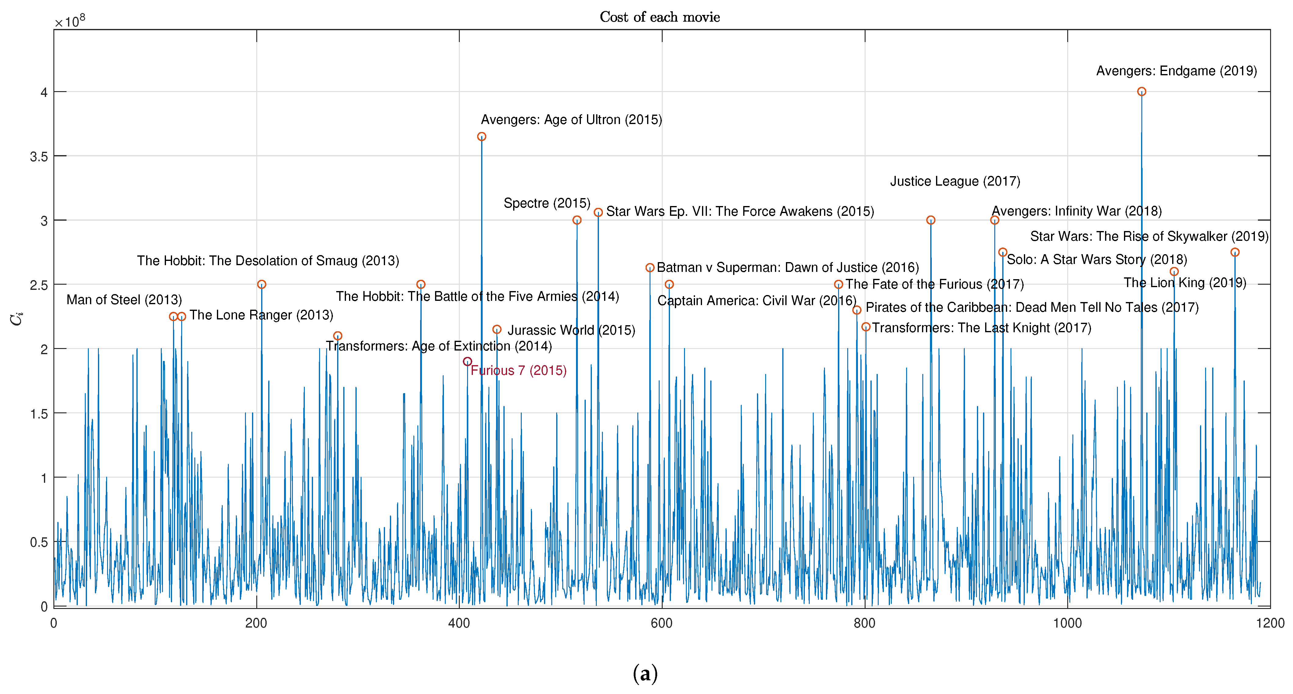
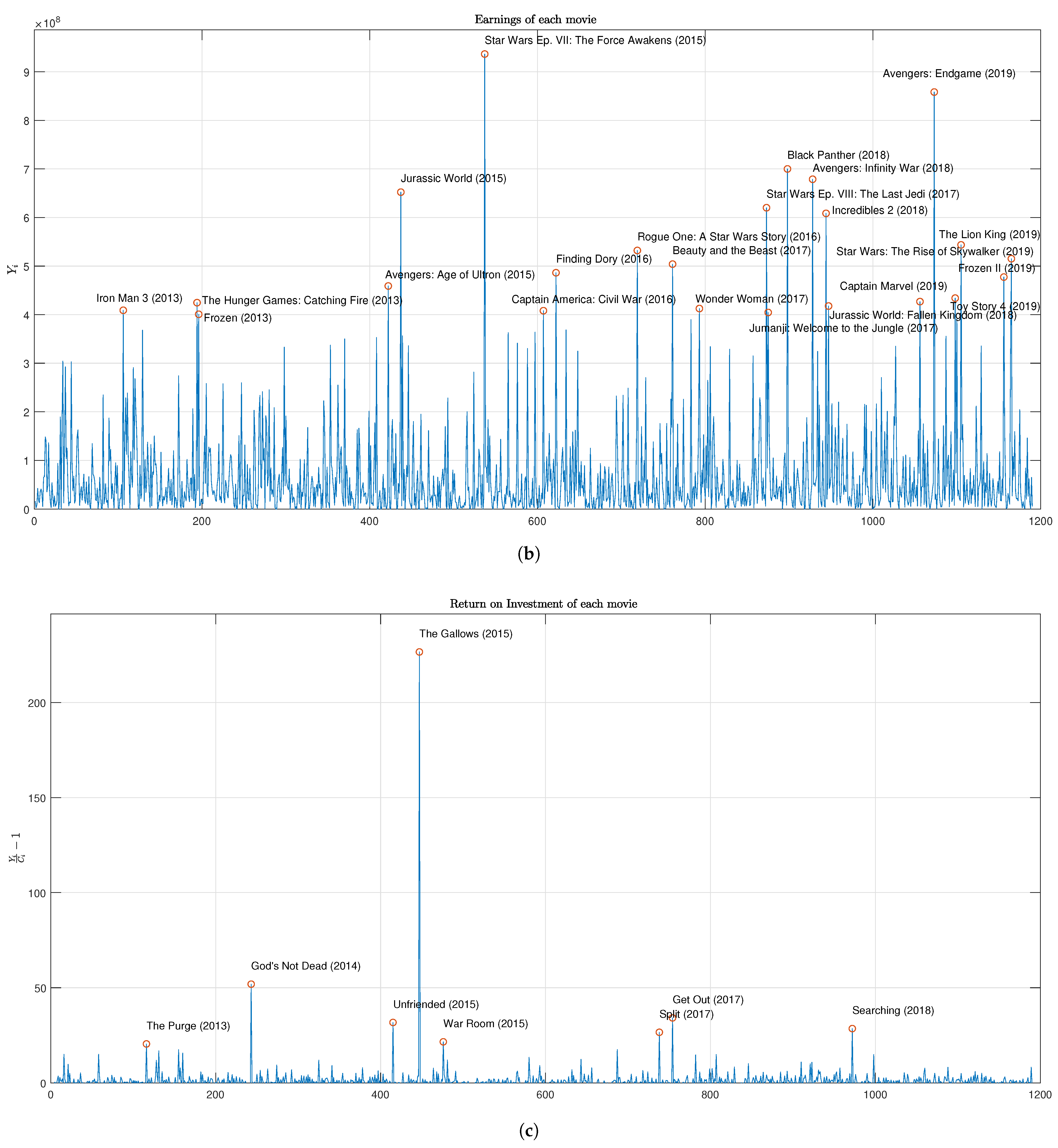
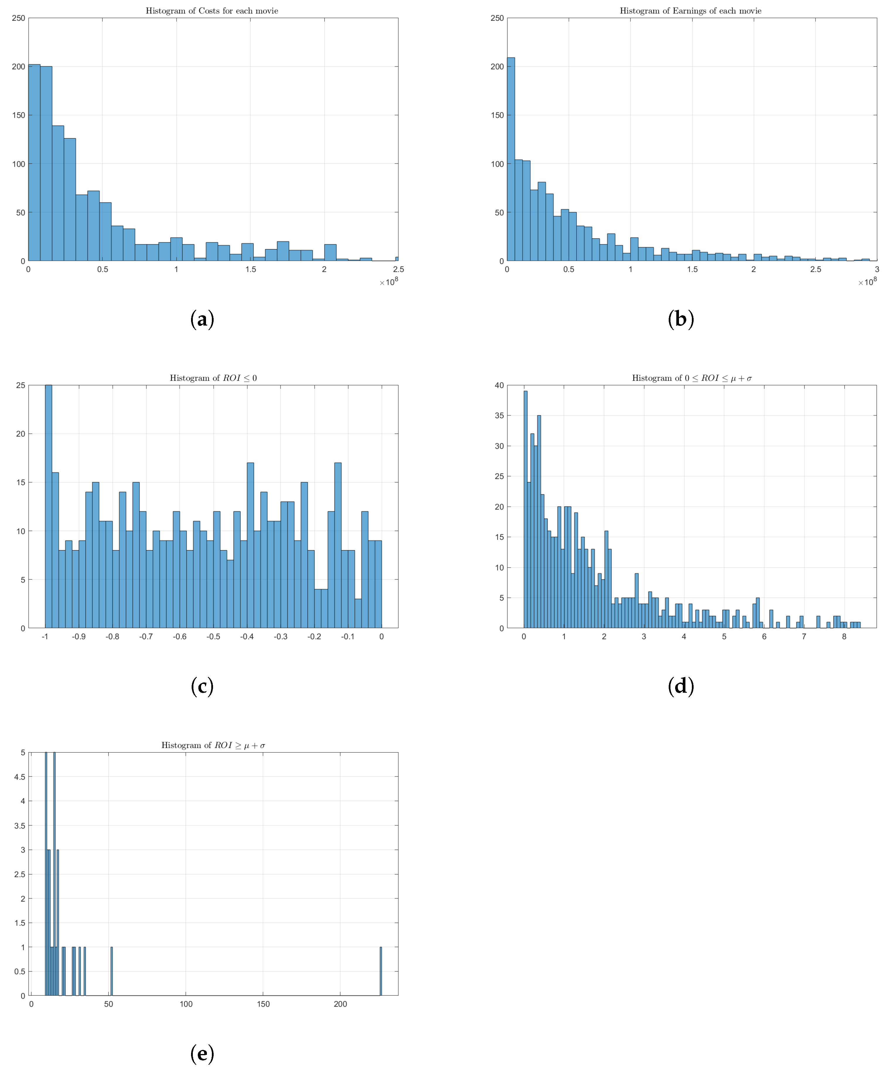
We show $C_i$ and $Y_i$ values in panels (a) and (b) of Figure 1, labeling the outliers (values greater than the 0.99 quantile) with the title of the corresponding movie. Histograms are drawn in Figure 2 and the main statistics reported in

Table A1. Variables—Univariate Statistics.

Variable	Mean	Median	Std	Skewness	Kurtosis	${\mathbf{CVaR}}_{0.05}^{\left(\mathit{l}\right)}$	${\mathbf{CVaR}}_{0.95}^{\left(\mathit{u}\right)}$
C	$4.910\times {10}^7$	$2.600\times {10}^7$	$5.728\times {10}^7$	1.958	7.192	$1.342\times {10}^6$	$2.172\times {10}^8$
Y	$6.686\times {10}^7$	$3.070\times {10}^7$	$9.813\times {10}^7$	3.434	19.588	$2.043\times {10}^5$	$4.032\times {10}^8$
$ROI$	1.265	0.052	7.362	24.757	742.478	−0.970	15.595
L	−0.025	0.051	1.48184	−1.56301	9.39145	−4.22111	2.4781
$T_i$	77	73	40.0	0.732	4.294	9.409	173.821
$N_t$	34	34	4.6	0.120	2.875	25.331	43.506
$c_t$	$1.965\times {10}^7$	$1.974\times {10}^7$	$5.656\times {10}^6$	0.238	3.775	$8.528\times {10}^6$	$3.195\times {10}^7$
$y_t$	$2.568\times {10}^7$	$2.037\times {10}^7$	$1.925\times {10}^7$	1.083	4.237	$4.184\times {10}^6$	$7.395\times {10}^7$
$I_t$	4.125	4.080	0.810	0.461	3.420	2.725	5.950
$R_t$	$-1.931\times {10}^{-4}$	$-5.711\times {10}^{-4}$	0.165	0.399	3.900	−0.334	0.393

.

Total costs and domestic earnings have a sample mean of $4.91\times {10}^7$ and $6.69\times {10}^7$ dollars, and a standard deviation of $5.73\times {10}^7$ and $9.81\times {10}^7$ respectively. The pronounced variance is also accompanied with high positive values of skewness and kurtosis. The median of both the variables is considerably lower than the mean, confirming the substantial skewness toward the right. The leptokurtic shape of these two distributions has been extensively investigated, see De Vany (2004) and the references therein. The return on investment series inherits statistical properties from its constituents. The sample mean and the median are positive, although the latter is more than 20 times lower; the standard deviation is eight times the mean, and both skewness and kurtosis have tremendous values. $RO{I}_i$ values are plotted in panel (c) of Figure 1, with outstanding returns labeled with their movie titles. It is worth noting that none of the movies with exceptional returns also have exceptional total box-office earnings or production expenditures. This has been already noted by De Vany (2004): wildly profitable low-budget movies can have extremely high return on investments, yet their total earnings are still less than a typical big-budget movie. Exceptional results are in some cases higher than 30 times the mean value and 20 times the standard deviation value. We measured the tail risk (reward) by computing the conditional value at risk (CVaR) of the left (right) tail of the ROI’s distribution.5 Formally, given a random variable X with distribution function $F_X$, we define the $\alpha$ lower and upper CVaRs as

$$\begin{array}{cc}\hfill & {\mathrm{CVaR}}_{\alpha }^{\left(l\right)}\left(X\right):=\frac{1}{\alpha }{\int }_{x<F_X^{-1}\left(\alpha \right)}xd{F}_X\hfill \end{array}$$

(2)

$$\begin{array}{cc}\hfill & {\mathrm{CVaR}}_{\alpha }^{\left(u\right)}\left(X\right):=\frac{1}{1-\alpha }{\int }_{x>F_X^{-1}\left(\alpha \right)}xd{F}_X,\hfill \end{array}$$

(3)

respectively. For the ROI’s empirical distribution we obtained values ${\mathrm{CVaR}}_{0.05}^{\left(l\right)}\left(ROI\right)=-0.97$ and ${\mathrm{CVaR}}_{0.95}^{\left(u\right)}\left(ROI\right)=15.60$. This evidence confirms both the high level of risk embedded in a movie project—we have a probability of 5% to lose practically all the invested capital—and the potential for high rewards, with again a 5% probability of obtaining extremely high returns.

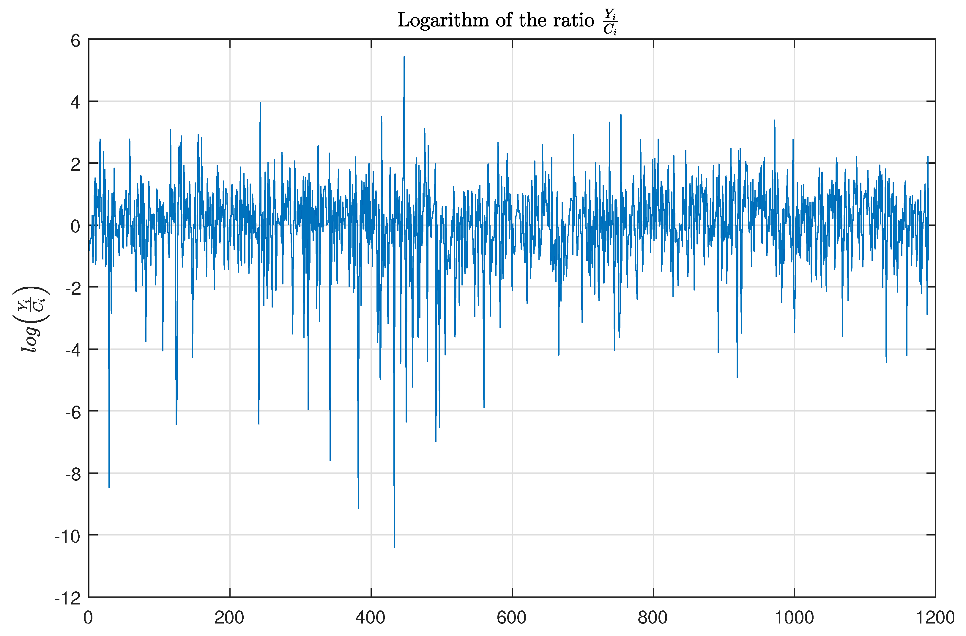
In order to see this more clearly, we have partitioned the data set into three subsets: (i) movies with negative returns $\left\{i:RO{I}_i<0\right\}$ and those with positive returns, which are further split into (ii) those either less than or (iii) greater than or equal to the mean ${\mu }_{ROI}$ plus the standard deviation ${\sigma }_{ROI}$, i.e., $\left\{i:0\le RO{I}_i<{\mu }_{ROI}+{\sigma }_r\right\}$ and $\left\{i:RO{I}_i\ge {\mu }_{ROI}+{\sigma }_{ROI}\right\}$. Histograms for the three sets are shown in Figure 2. We can see that in the case of the negative returns in panel (c), the distribution is more uniform and the complete failure, i.e., $RO{I}_i$ between $-0.98$ to $-1$, has the highest frequency. On the contrary, positive returns exhibit a distribution with persistent right tail, as is evident from panels (d)–(e). Since the return on investment is, by construction, limited below by −1 (null gross return) and virtually unbounded above, this leads to a strong asymmetry between the two tails and we apply the natural logarithm transform to $1+ROI$

$$L=ln(1+ROI)=ln\left(\frac{Y}{C}\right).$$

(4)

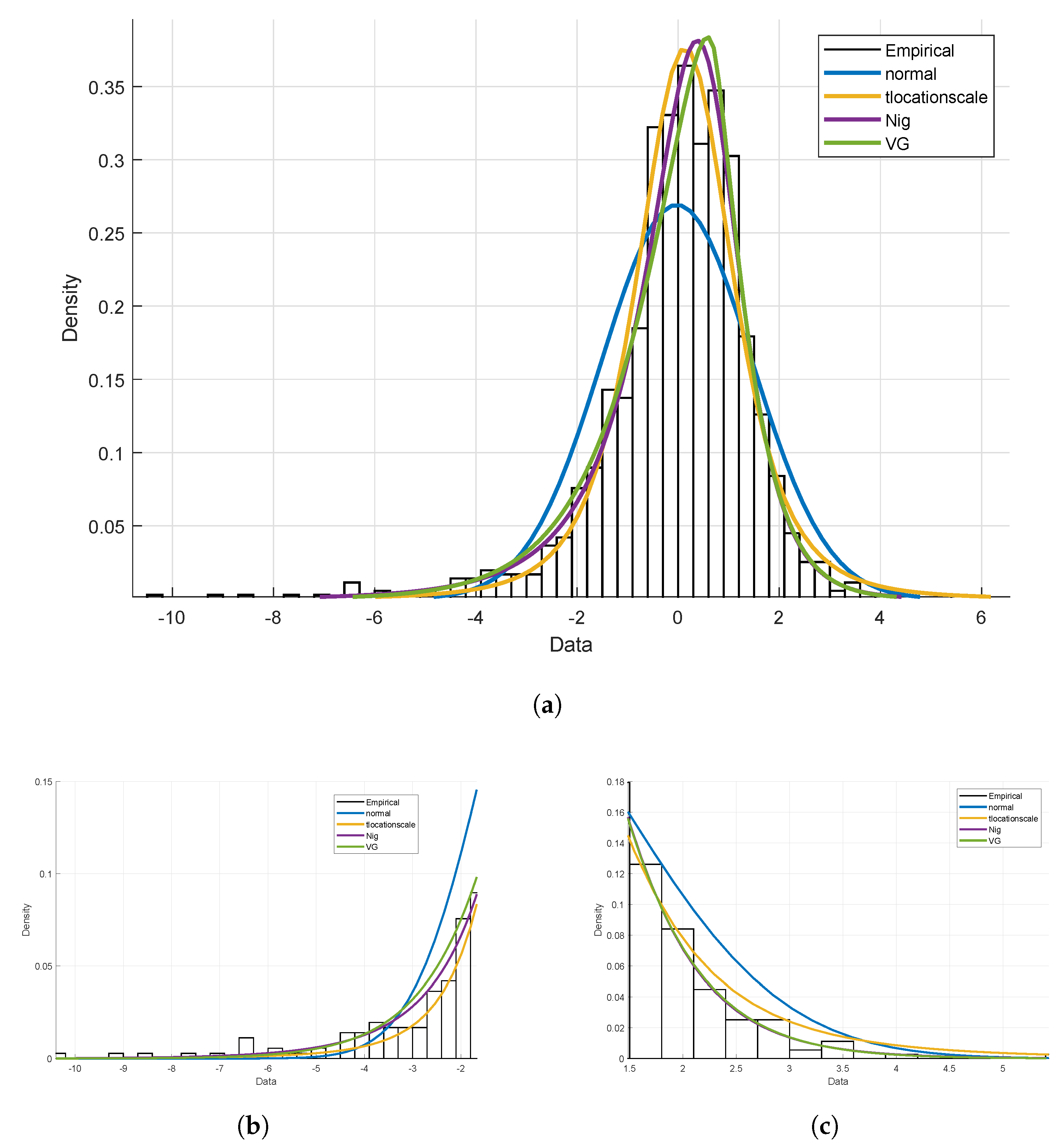
The logarithmic transformation mitigates the kurtosis, which is still substantially greater than the Normal case, and reverses the asymmetry: variable L has more probability mass in the left than in the right tail—see Table A1 and Figure 3. De Vany observed that the distributions of box-office earnings and returns on investment exhibit heavy upper tails decreasing at a power rate and both can be modeled by a Lévy Stable distribution De Vany and Walls (2004). In this work, we prefer to model return on investment by means of distributions belonging to the class of Generalized Hyperbolic (GH) distribution. This choice is motivated by the fact that GH distributions are, in general, more tractable than the Lévy Stable case, with well-defined and not infinite expected value and variance. The GH class has been introduced by Barndorff-Nielsen (1977) in order to study regularities in the distribution of aeolian sand deposits. In particular, a random variable X follows a GH distribution if its density function is given by

$$\begin{array}{cc}\hfill & f_X\left(x\right)=\frac{{\left({\alpha }^2-{\beta }^2\right)}^{\frac{\lambda }{2}}}{{\left(2\pi \right)}^{\frac{1}{2}}{\alpha }^{\lambda -\frac{1}{2}}{\delta }^{\lambda }{K}_{\lambda }\left(\delta \sqrt{{\alpha }^2-{\beta }^2}\right)}\frac{K_{\lambda -\frac{1}{2}}\left(\alpha \sqrt{{\left(x-\mu \right)}^2+{\delta }^2}\right)}{{\left({\left(x-\mu \right)}^2+{\delta }^2\right)}^{\frac{1-2\lambda }{4}}}{e}^{\beta \left(x-\mu \right)}\hfill \end{array}$$

(5)

where $K_{\nu }$ denotes the modified Bessel function of the third kind. The parameter $\mu$ states the location, $\alpha$ the shape, $\beta$ and $\delta$ are a skewness and a scaling parameter respectively, and $\lambda$ governs the tail heaviness. Parameters have to satisfy the constraints $\lambda ,\mu \in \mathbb{R}$ and

$$\begin{array}{cc}\hfill & \delta \ge 0,0\le \left|\beta \right|<\alpha ,\mathrm{if}\lambda >0,\hfill \\ \hfill & \delta >0,0\le \left|\beta \right|<\alpha ,\mathrm{if}\lambda =0,\hfill \\ \hfill & \delta >0,0\le \left|\beta \right|\le \alpha ,\mathrm{if}\lambda <0.\hfill \end{array}$$

This class contains, for particular choices of the parameters’ values, both distributions with semiheavy tails—for instance the normal inverse Gaussian (NIG) and the variance-gamma (VG)—and distribution with heavy tails, t-Student, and Cauchy. These features, along with their flexibility to model asymmetries in the shape of distribution, have attracted attention to this class, which have been extensively applied in finance, see for instance Barndorff-Nielsen (1997a, 1997b); Madan and Seneta (1990); Eberlein and Keller (1995). The NIG distribution turns out to be the best fit for the empirical distribution of variable L, according to the Akaike information criterion (AIC), as shown in panels (b)–(c) of Figure 4; estimated parameters are reported in

Table A2. Estimated parameter values of different distributions belonging to the Generalized Hyperbolic class and corresponding values of the Akaike information criterion AIC and the log likelihood value llh.

Variable	Distribution	$\mathit{\lambda }$	$\mathit{\alpha }$	$\mathit{\mu }$	$\mathit{\beta }$	$\mathit{\delta }$	AIC	llh
L	t	−2.382	0.402	0.647	−0.402	2.162	4030.353	−2009.176
	NIG	−0.500	0.860	0.616	−0.374	1.327	4029.683	−2010.841
	VG	1.596	1.456	0.716	−0.446	0	4049.633	−2020.816
$h_t$	t	−1.795	0.265	−0.265	0.265	1.265	1975.550	−983.7748
	NIG	−0.500	0.917	−0.265	0.270	0.814	1973.332	−982.6660
	VG	1.370	1.791	−0.310	0.334	0	1980.610	−986.3052

.

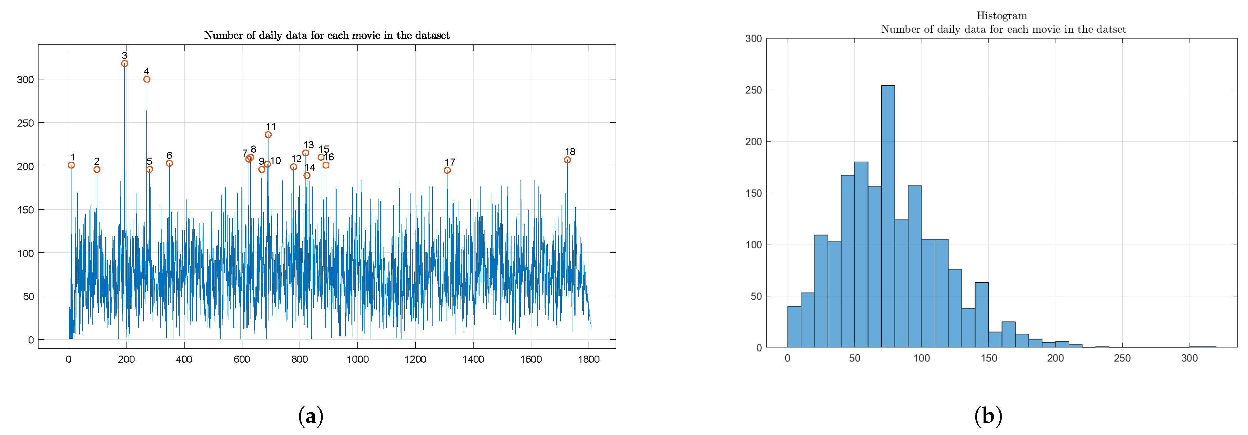
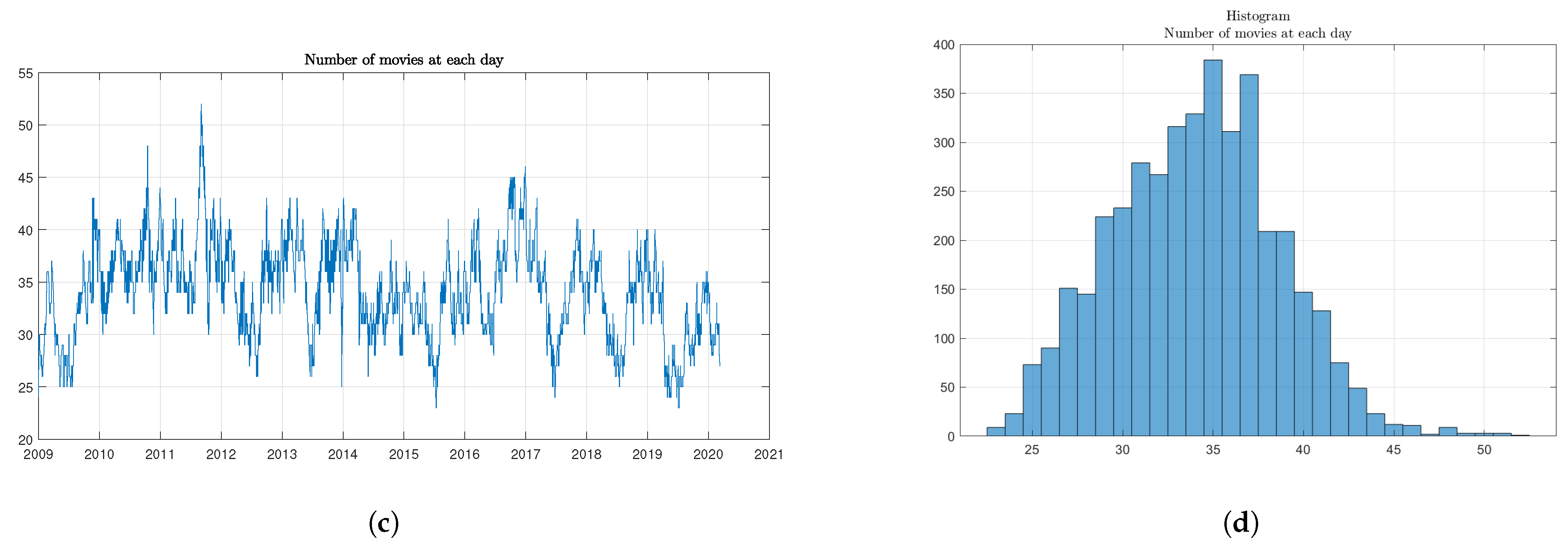
So far we have considered total quantities, providing useful statistical information on costs, earnings, and return on investment for each movie. Now we move the analysis toward a daily basis, which is motivated in large part by the approach to tracking box office data that has long been practiced by the film industry itself. We start by investigating statistical features of the set of series ${\left\{y_{i,t}\right\}}_{t={\tau }_{s,i}}^{{\tau }_{e,i}}$, for $i=1,\dots ,N$. We do not have a standard, consistent number of daily observations for each movie but rather each film possesses a different total number of daily box-office earnings, as shown in panels (a) and (c) of Figure 5. This is primarily due to the fact that movies stay in theaters for different periods, though also perhaps a result of missing values in the data set. In our data set, a movie stays in theaters 80 days in mean with a standard deviation equal to 40 days. The empirical probability of having more than 30 daily data for a movie is $0.8866$, so that we are quite confident that we have sufficient data to construct the index. Another issue concerns the number of movies $N_t$ shown in theaters at date t. The plot of $N_t$ and its histogram for every date in the data set is plotted in Figure 5—panels (b) and (d). In the data set there are in mean 34 movies at each date with a standard deviation of 4.56; in 95% percent of dates, $N_t$ is between 25 and 41, so we can confirm that the data set contains a relatively stable amount of daily data. The dynamic of $N\left(t\right)$ shows evident downturns during the summer and picks up in the late fall and during Christmas holidays.

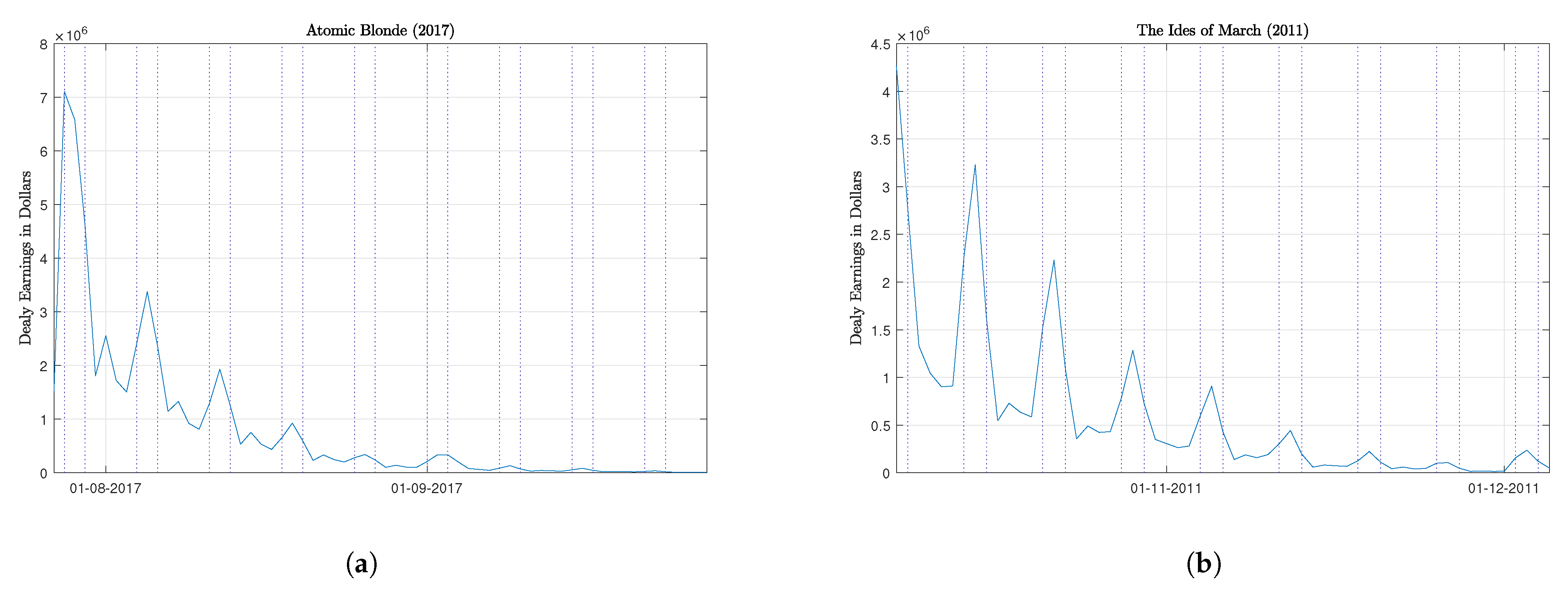
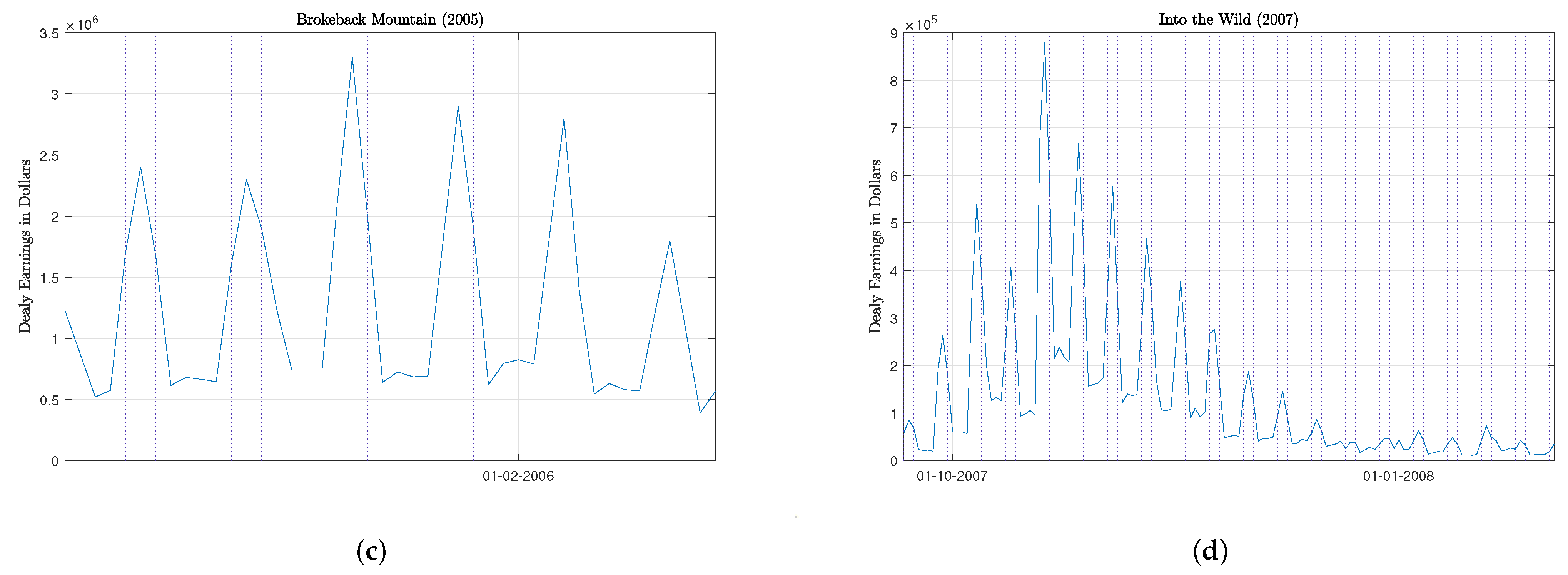
Figure 6 contains the graph of the series ${\left\{y_{i,t}\right\}}_{t={\tau }_{s,i}}^{{\tau }_{e,i}}$ for four different movies, selected from different years. A common feature that emerges is a weekly seasonality: from Friday to Sunday daily box-office revenues increase to a great extent with respect to the value before the weekend; a small increment every Tuesday is also noted, likely due to ticket discounts. We can observe two different sinusoidal pattern categories: in the first, high returns occur in the first weeks with a gradual decay with time, see panels (a)–(b); in the second, instead, we observe weekend returns gradually increasing at first before also beginning to decay, as shown in panels (c)–(d).

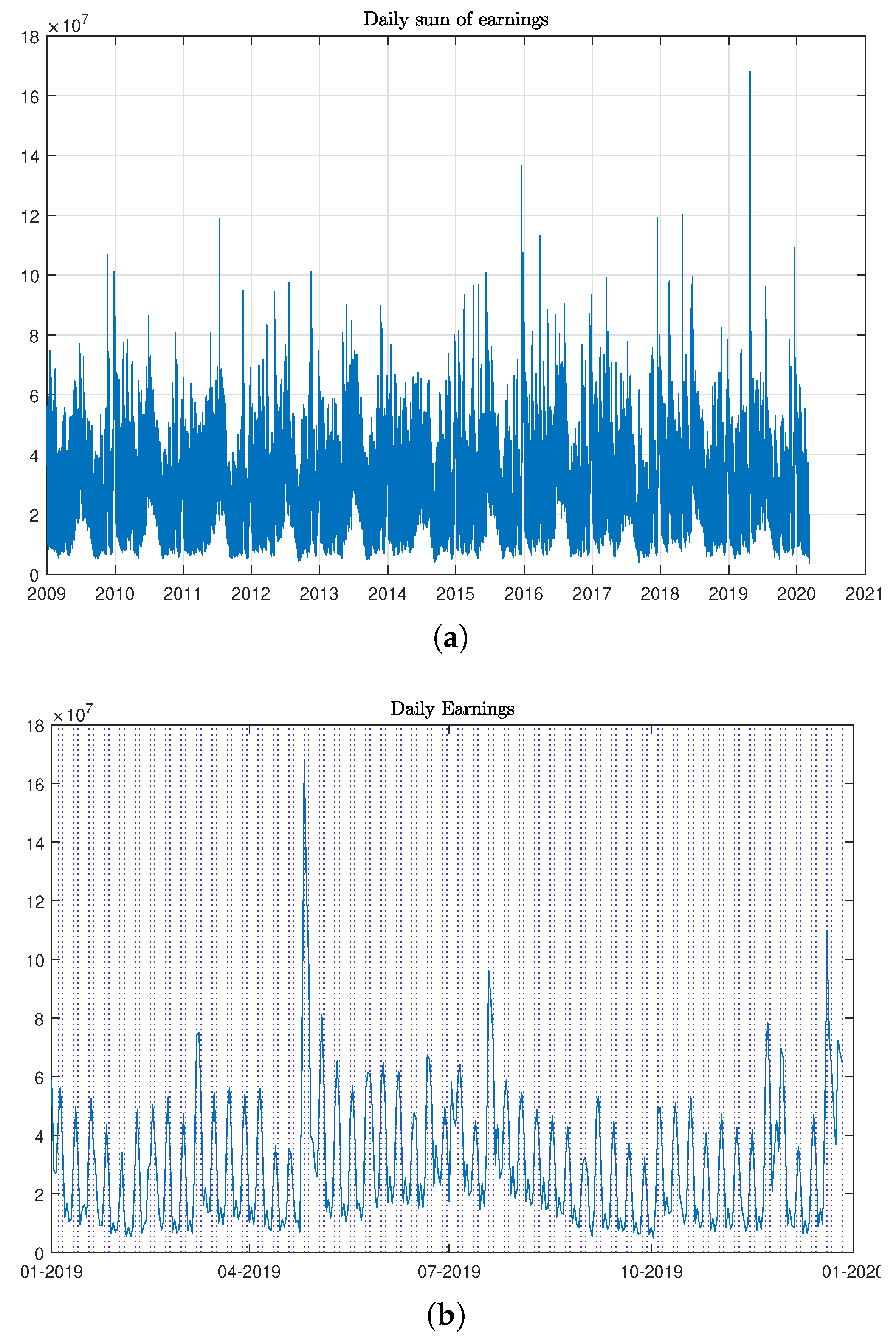
Let us now consider the aggregate value of daily box-office earnings $y_t:={\sum }_{i=1}^{N_t}{y}_{i,t}$. The whole series is depicted in panel (a) of Figure 7; in panel (b) we instead show the trajectory specific to 2019. It is easy to see that the series preserves the weekly seasonality of its addend, with the highest upward spikes falling on the weekends and the small spikes on Tuesdays. By looking at the graph in panel (a), we also recognize a yearly seasonal pattern in the series: a large and short increase during the Christmas holidays and a smaller but longer appreciation during the summer.

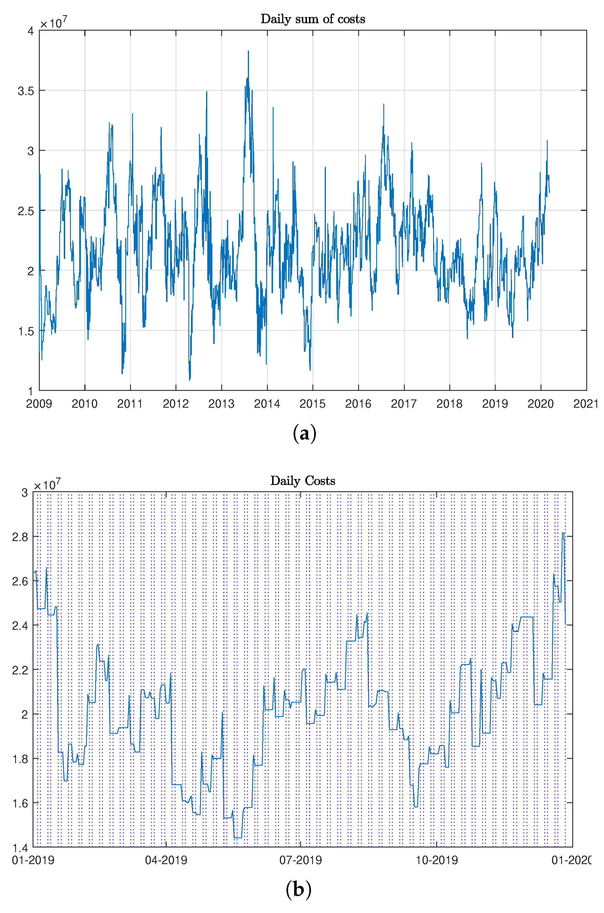
In order to define an aggregate measure of daily returns for the whole industry, we would like to have a daily and aggregate measure of the cost of production for every movie in theaters on that date. We first define $T_i$ as the number of daily box office data for the i-th movie, and then we amortize the total cost of the single movie i on a daily basis by taking the ratio between its total cost $C_i$ and $T_i$. The ratio $\frac{C_i}{T_i}$ is the daily cost contribution to the overall production expenditure.6 The aggregate daily cost $c_t$ will be then computed as the sum of these ratios: $c_i:={\sum }_{i=1}^{N_t}\frac{C_i}{T_i}$. Analogously with what we have done in Figure 7 for the aggregate series of box-office earnings, we plot the whole aggregate cost series in panel (a) of Figure 8, and in panel (b) the series during the year 2019.

3. Movie Returns Index

3.1. The Basic Economics of Hollywood—Part I

The bedrock upon which Classical Hollywood Cinema thrived from the late 1920s through the end of World War II was vertical integration, with major studios owning production companies, distribution arms, and key sites of exhibition (retail). Funding for these companies came primarily in the form of corporate financing from Wall Street. Bank loans were extended against real estate holdings, primarily their downtown urban theaters Landry and Greenwald (2018). In 1948, this strategy of vertical integration was struck down by the U.S. Supreme Court and the studios were forced to sell the theaters, losing as a result their principal form of collateral King (2012). At the same time, post-war audiences shrank from a high of four billion admissions in 1946 to a low of one billion in 1970, undermining the large rates of return the movie studios had previously enjoyed. As a result, Hollywood was forced to seek alternative funding models Sedgwick (2002). Selling out to corporate conglomerates which could generate operating income and offer production funds through other types of businesses or secure debt financing by offering other holdings as collateral became a viable option; the 1960s is littered with such moves Schatz (2008).

As the number of productions was reduced in response to the shrinking market, the risk associated with each film rose. In addition, media and entertainment competition continued to be high as color televisions moved into a majority of homes by the early 1970s. Poorly reviewed films, especially the expensive ones, lost buckets of money. Increasingly the industry witnessed a shift in attendance around “event” films or blockbusters. Jaws (1975) changed the way films were advertised to the American people, focusing now on large investments in television spots in preparation for a high-volume opening weekend built around “saturation” releases. The success of Star Wars two years later further cemented the ROI capacities for certain films released in this manner. The new policies of saturation release—opening a film in as many theaters across the nation at the same time as possible—and a coordinated marketing blitz could still sell tickets before bad word of mouth spread to kill a film’s chances Hall and Neale (2010). This new blockbuster-based industry became increasingly evident during the 1980s and has dominated market structures ever since Wyatt (2015).

Economists inside and outside of Hollywood have studied the resulting patterns. Though for Hollywood productions “the total mean box office exceeds the mean production costs” Simonton (2009), “the distribution of motion picture revenues is highly skewed, and”—as we have already discussed—“the mean is dominated by a few movies in the extreme tail” De Vany and Walls (2002). As a result, industry wisdom posits something along the lines that, out of ten releases, seven will lose money or break even at the box office and three will profit, with one of those being so successful with audiences that its ROI makes up for all the others plus a nice overall profit. Still, film studios never know exactly which movie in their slate will rise to the status of such a moneymaker, so the industry overall adopted production strategies that the film companies collectively recognized, based on this business model of a few blockbuster smashes, would best facilitate their chance for success.7 The high risk/high reward nature of investment in the American motion picture industry that was exacerbated as a result of this change has now been significant for so long that the familiar adage “nobody knows anything”—first phrased as such by Hollywood screenwriter William Goldman in his 1983 book Adventures in the Screen Trade—has been adopted into the “nobody knows principle” by economists such as Richard Caves. According to Caves, “producers and executives know a great deal about what has succeeded commercially in the past and constantly seek to extrapolate that knowledge to new projects. But their ability to predict at an early stage the commercial success of a new film project is almost nonexistent” Caves (2000).8 However, though the risks associated with each and every film may be high, the breadth and depth of the industry and the overall demand for their product has resulted in a general stability with regular growth and often-rewarding investment options.

According to Peter Dekom, a Los Angeles-based entertainment lawyer, uninitiated film investors seeking high-risk opportunities expect rates of return in the 25–30% range. Like many of the films produced in Hollywood, such numbers are very close to pure fantasy. Prior to COVID-19, the motion picture business generated expected, internal rates of return between minus 20% and 20%, with the average from 2010 to 2015 for the major studios (which account for the vast majority of the domestic box office) in the range of 10–15%. Independent film companies set up to produce a single film or even one film at a time allow for direct investment opportunities, but the risk is fully on the performance of that single film and the track record here is remarkably poor and “the percentages are very often negative” Dekom (2017). Still, the popular notion that with deep enough pockets and the right connections investing in a wildly successful film can be possible pushes motion picture producers to sell the dream and drives wealthy financiers to wade into the ridiculously high-risk waters. They call it La-La-Land for a reason.

In addition, profiting from an investment in a single film is never the result of a simple return on investment (ROI) calculation: production (or “negative”) cost subtracted from total box office. The film’s producers split box office revenues with first the exhibitor and then the distributor (hence Hollywood’s early move toward vertical integration). Most exhibition contracts are designed on a sliding scale that benefits distributors early—as much as 90/10 during the opening weekend—and exhibitors later (generally around 70/30) during a film’s period of theatrical release Filson et al. (2005).9 P&A, or Prints & Advertising (of which advertising takes up the vast majority), also have to be deducted, generally from the distributor’s take, as they do not count toward a film’s budget. The received wisdom is that large marketing budgets act like a loss leader, costing significantly up front in order to generate advance notice of not just a film’s theatrical release but its entire run through all ancillary markets. These traditionally begin with the international theatrical market and continue through video-on-demand (VOD) and the shrinking but still breathing home video/DVD market, each of which plays a key role in determining the ultimate profitability (or not) of an individual motion picture. Television licensing rights, licensing to streaming services (Over the Top or OTT platforms), music publishing and soundtrack sales, and merchandising and marketing licenses (toys, lunchboxes, clothes, etc.) round out the typical ancillary markets. There is no exact correlation between production budget and advertising dollars, but risk aversion tends to dictate a soft relation between the two and industry wisdom indicates that the marketing budget is usually equal to half of the production budget, particularly on larger-budget films with greater investment at risk Landry and Greenwald (2018). Even films that lose money at the domestic box office have the potential to be ultimate money-makers for their producers, depending on the value of licensing rights, the extent of merchandising, etc. All of these ancillary markets are part of a film’s income over its life and the range of ancillary markets leveraged advantageously often dictates whether an individual title is profitable or not. As a result of the inherent “trickle down” logic of these traditionally ancillary markets, the overall health and performance of the industry has generally been monitored via the success of the domestic box office, even as this represented an increasingly smaller portion of the overall gross profits. ROI then offers, despite its incomplete reflection of an individual film’s profitability, a direct means of tracking such industry-level box office performance.

3.2. Index Construction

The scope of this part of the section is twofold. Firstly, we construct an index which describes the time evolution of returns in the whole U.S. movie industry on a daily basis. Then, we present a time-discrete series model that can be efficiently used to model and forecast index returns. Given the daily series $y_{i,t}$ and $c_{i,t}$ introduced in Section 2, the aggregate daily rate of return $r_t$ at t can be defined as the sum of individual rates $r_{i,t}:=\frac{y_{i,t}}{c_{i,t}}$, so that we can write $r_t:={\sum }_{i=1}^{N_t}\frac{y_{i,t}}{c_{i,t}}$. This quantity is bounded below by zero and potentially unbounded from above, and, as shown in the previous section, the fat tails of earnings and cost distributions produced a similar distribution for the series $r_t$. Following the same motivations as the $ROI$ analysis, we consider the natural logarithm transformation of $r_t$, and the aggregate daily index can be defined by:

$$I_t=log\left(\sum _{i=1}^{N_t}\frac{y_{i,t}}{c_{i,t}}\right).$$

(6)

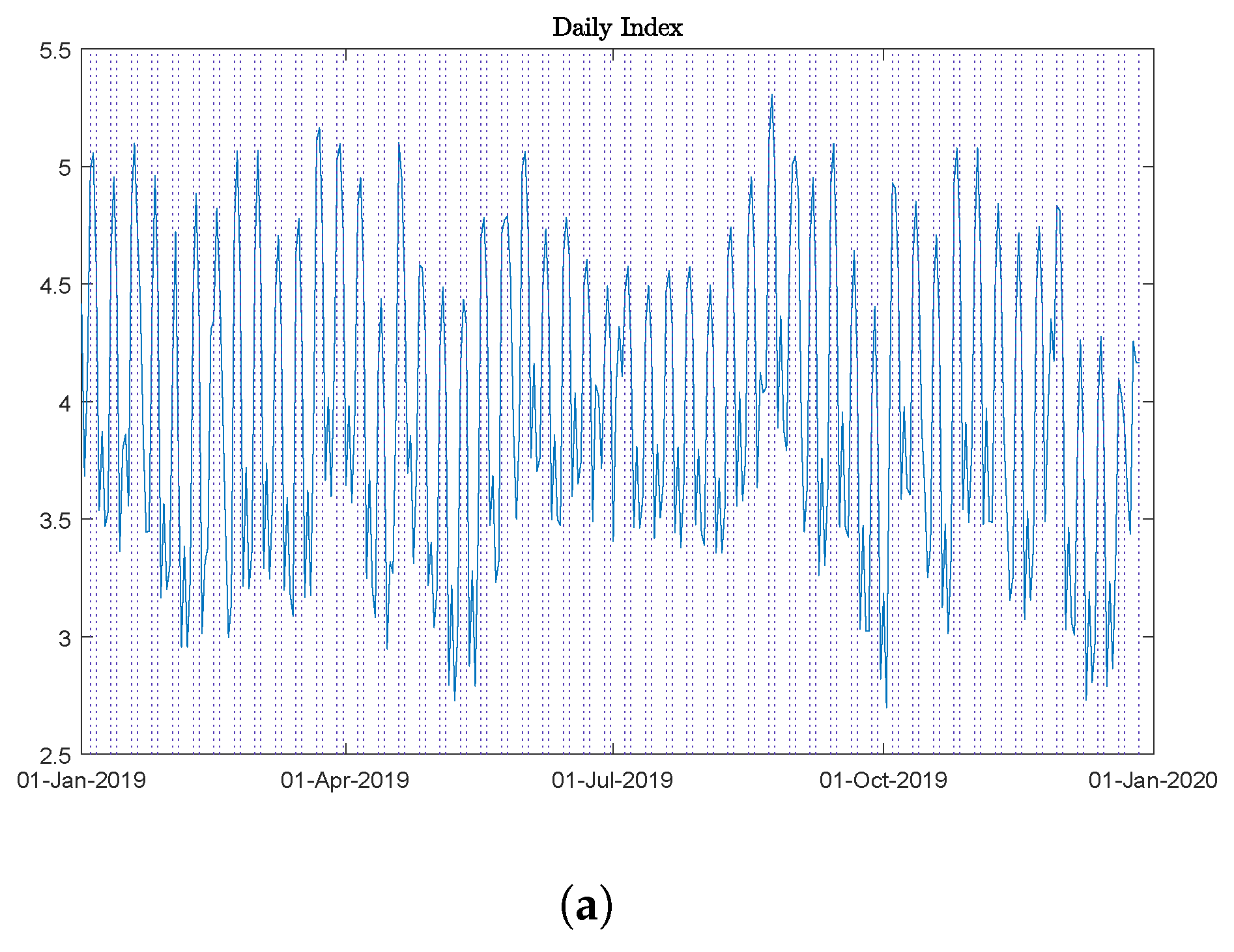
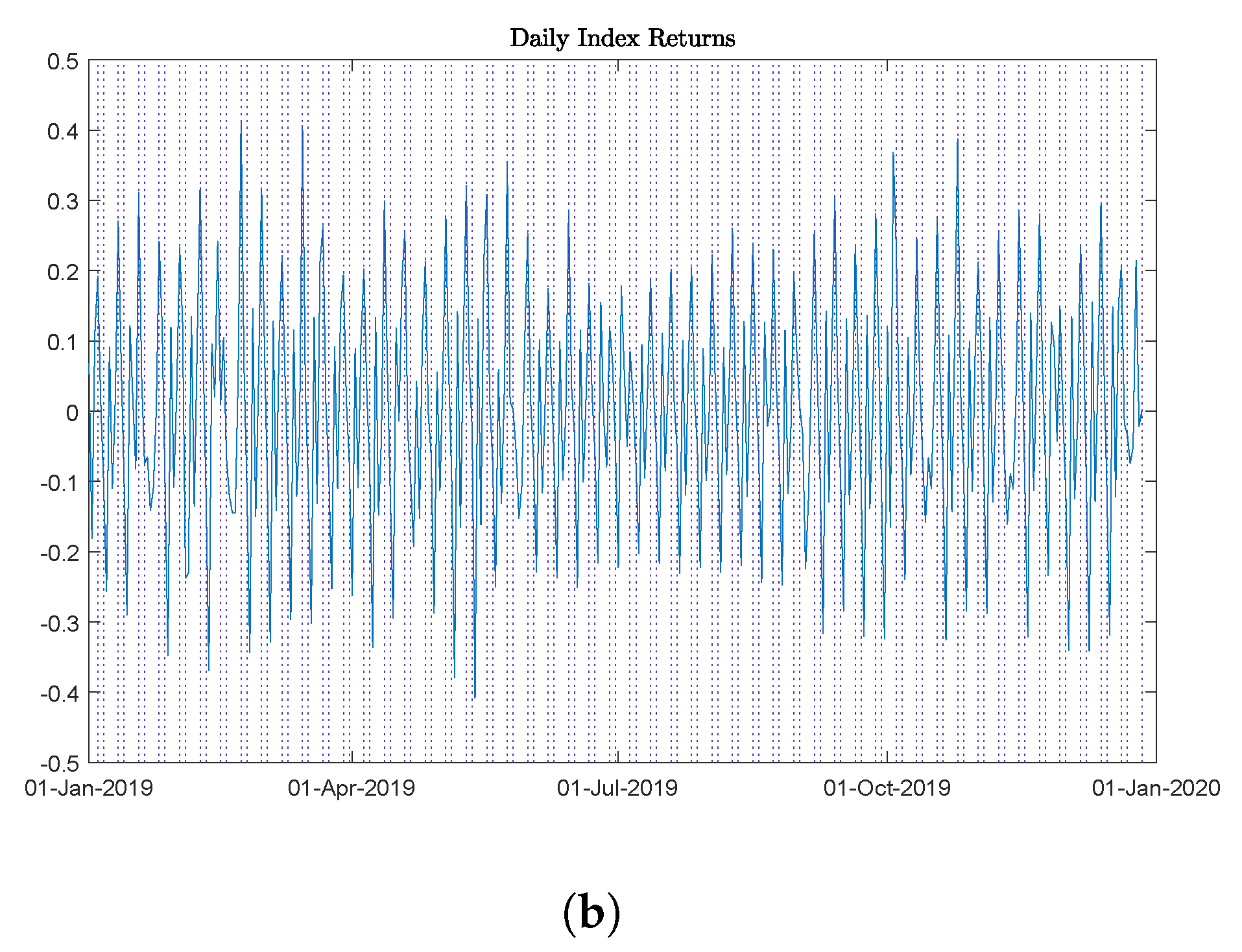
The value $I_t$ is a measure of the global ROI realized at t, providing specific business information that is uniquely related to a particular market day.10 The index has been computed by considering all of the movies in theatrical release and, as such, it should be regarded as a reference for the whole industry. Daily simple returns on the index can then be defined as $R_t=\frac{I_{t+1}-I_t}{I_t}.$ The index price $I_t$ and index returns $R_t$ are plotted in Figure 9 for the entire period 1 January 2009 to 10 March 2020,11 and in Figure 10 only for 2019 in order to better visualize intrayear seasonal cycles.

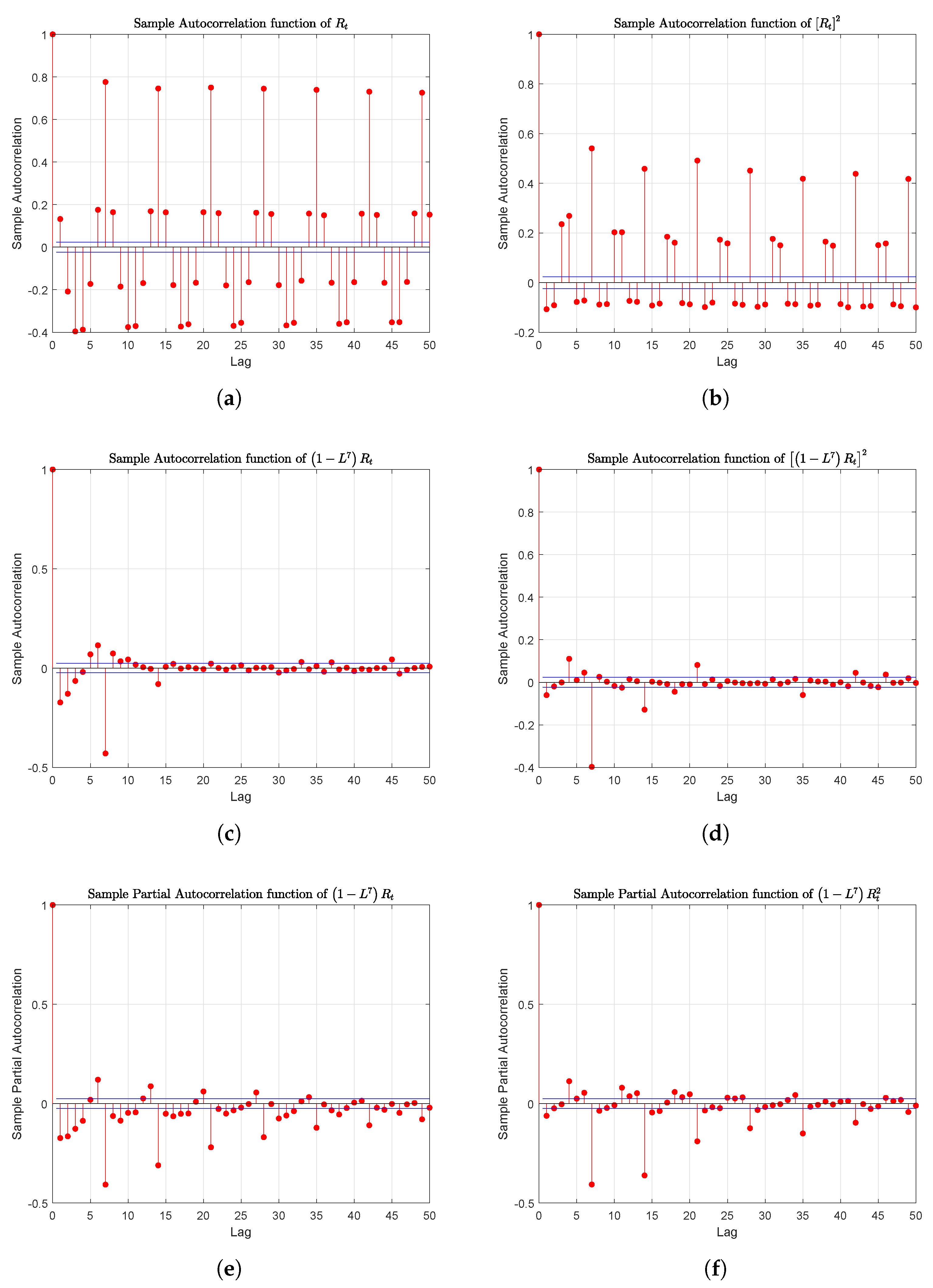
Looking at Table A1, we can see that the skewness of $I_t$ and $R_t$ is 0.46 and 0.40 and kurtosis values are 3.42 and 3.90 respectively: the logarithm transformation, which rescales the index to the entire real line $\mathbb{R}$, has smoothed extraordinary returns reducing both skewness and kurtosis, which, in any case, are still greater than the Gaussian case. Seasonality features of daily box-office revenues are transmitted to the index $I_t$, with the Weekend and Tuesday effects previously illustrated. We expect to find these seasonal components also in the return series $R_t$. This is confirmed by the behavior of its empirical autocorrelation function, which exhibits a periodical cycle with highest peaks at lags of seven day intervals—see panel (a) in Figure 11.

The values of these peaks do not decrease with time, but they look substantially unchanged, suggesting a nonstationarity feature. We test the stationarity of the series by means of the Kwiatkowski, Phillips, Schmidt and Shin test Kwiatkowski et al. (1992), for lags between 1 and 7 and with a p-value of 0.01: the test rejects the null of stationarity; the same result has been confirmed by the Hylleberg, Engle, Granger and Yoo (HEGY) test statistics for the null hypothesis seasonal unit roots Hylleberg et al. (1990).

We also detected an autoregressive seasonal component in the conditional variance, which clearly emerges by looking at the sample autocorrelation function of the squared series $R_t^2$, Figure 11, panel (b). In order to transform the original series of returns into a stationary process, we apply a difference filter of order seven. The empirical autocorrelation and partial autocorrelation functions of the new series $\left(1-L^7\right)R_t$ and of its square ${\left[\left(1-L^7\right)R_t\right]}^2$—shown in Figure 11, panels (c)–(f)—quickly decrease with a sinusoidal pattern, but with a single spike at the seventh lag, suggesting that both the conditional mean and the conditional variance are governed by a seasonal autoregressive and mean average process.

We have fitted several SARIMA-GARCH models on $\left\{R_t\right\}$,12 under the assumptions of NIG innovations, and then selected the best model according to three features: the degree of autocorrelation in the standardized residual series, the two information indexes AIC and BIC, and the mean square error (MSE) between the model response and real data. We have first estimated the model supposing t to be at 1 June 2019 on a time window of two years (730 data points). According to this approach, we find that the best model for the conditional mean component is the SARIMA(2,0,2)×(7,7,7), whereas the conditional variance follows an ARCH model with two lags of orders one and seven. By introducing the lag operator L and the error process $\left\{{ϵ}_t\right\}$ with zero mean and variance ${\sigma }_t^2$, the time series model can be formally defined by the two processes

$$\left(1-{\alpha }_{1}L-{\alpha }_2{L}^2\right)\left(1-\varphi L^7\right)\left(1-L^7\right)R_t=\left(1+{\beta }_1+{\beta }_2{L}^2\right)\left(1+\psi L^7\right){ϵ}_t,$$

(7)

$${\sigma }_t^2={\gamma }_1{ϵ}_{t-1}^2+{\gamma }_7{ϵ}_{t-7}^2,$$

(8)

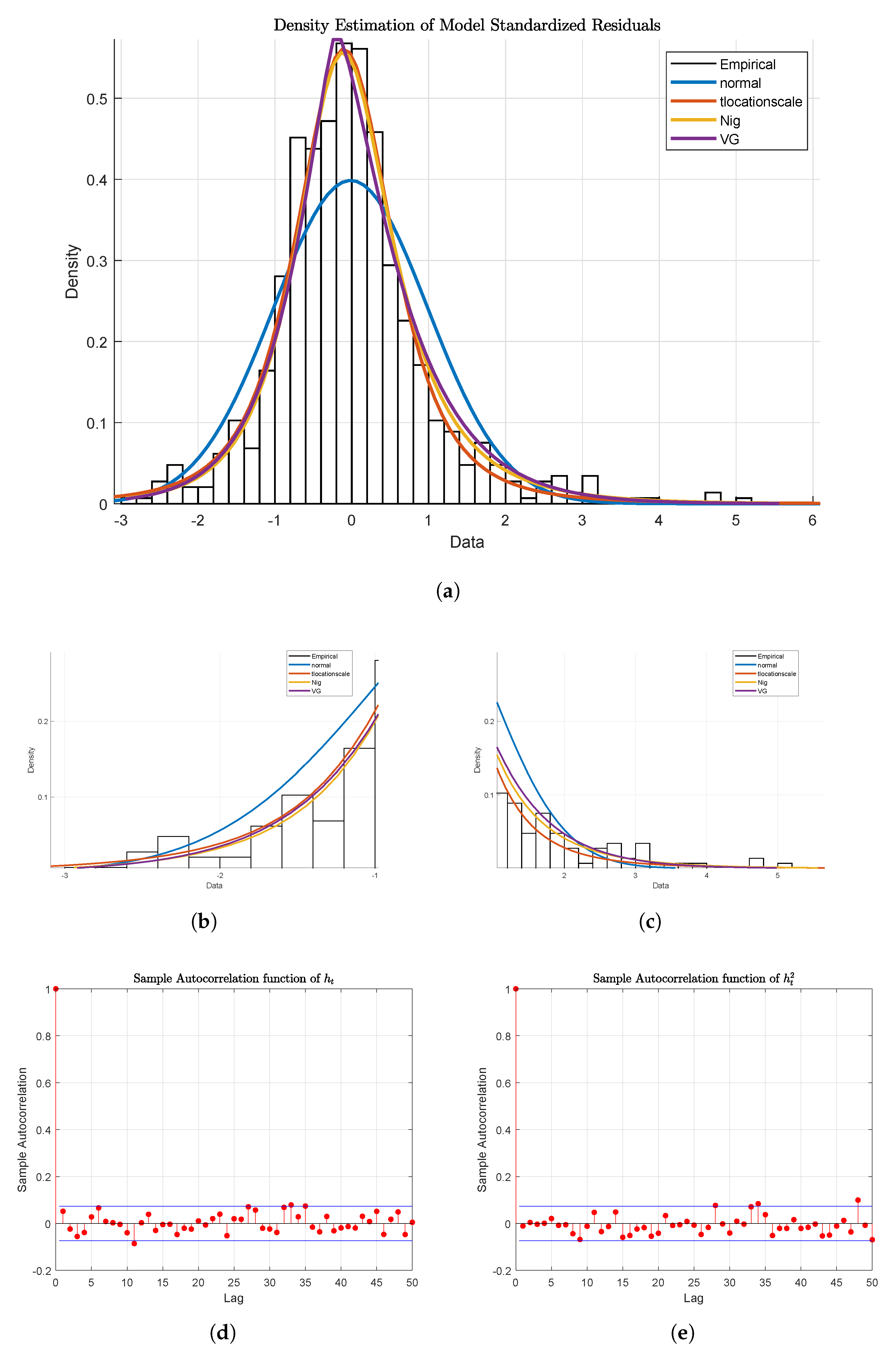
where the former describe the evolution of the conditional mean and the latter the conditional variance process. Model parameters with corresponding p-values and the mean square error are shown in

Table A3. Parameter values and corresponding p-values for the SARIMA-GARCH model (7)–(8).

Conditional Mean	${\mathit{\alpha }}_1$	${\mathit{\alpha }}_2$	${\mathit{\beta }}_1$	${\mathit{\beta }}_2$	$\mathit{\varphi }$	$\mathit{\psi }$
Value	−1.522366	0.351508	0.211057	−1.679167	0.103901	−1.878299
p-Value	$4.2721\times {10}^{-8}$	$3.2764\times {10}^{-6}$	0.010639	$7.4738\times {10}^{-21}$	0.01374	0
Conditional Variance	${\gamma }_1$	${\gamma }_7$
Value	0.29719	0.17737
p-Value	$1.6505\times {10}^{-8}$	0.00030031
Model Measures	AIC.	BIC	MSE	MSPE
	−1.43.	−1.7	0.0047	0.0116

. Model validation has been conducted in three ways. First we looked at the sample autocorrelation functions of standardized residuals $h_t:=\frac{{ϵ}_t}{{\sigma }_t}$ and their square $h_t^2$—Figure 12, panels (d)–(e): all the values of the two functions are lower than the significative level for lags greater than one. In the same figure, panels (a)–(c), we show density fits for the standardized residuals with Normal, Normal Inverse Gaussian, and Variance-Gamma distributions.

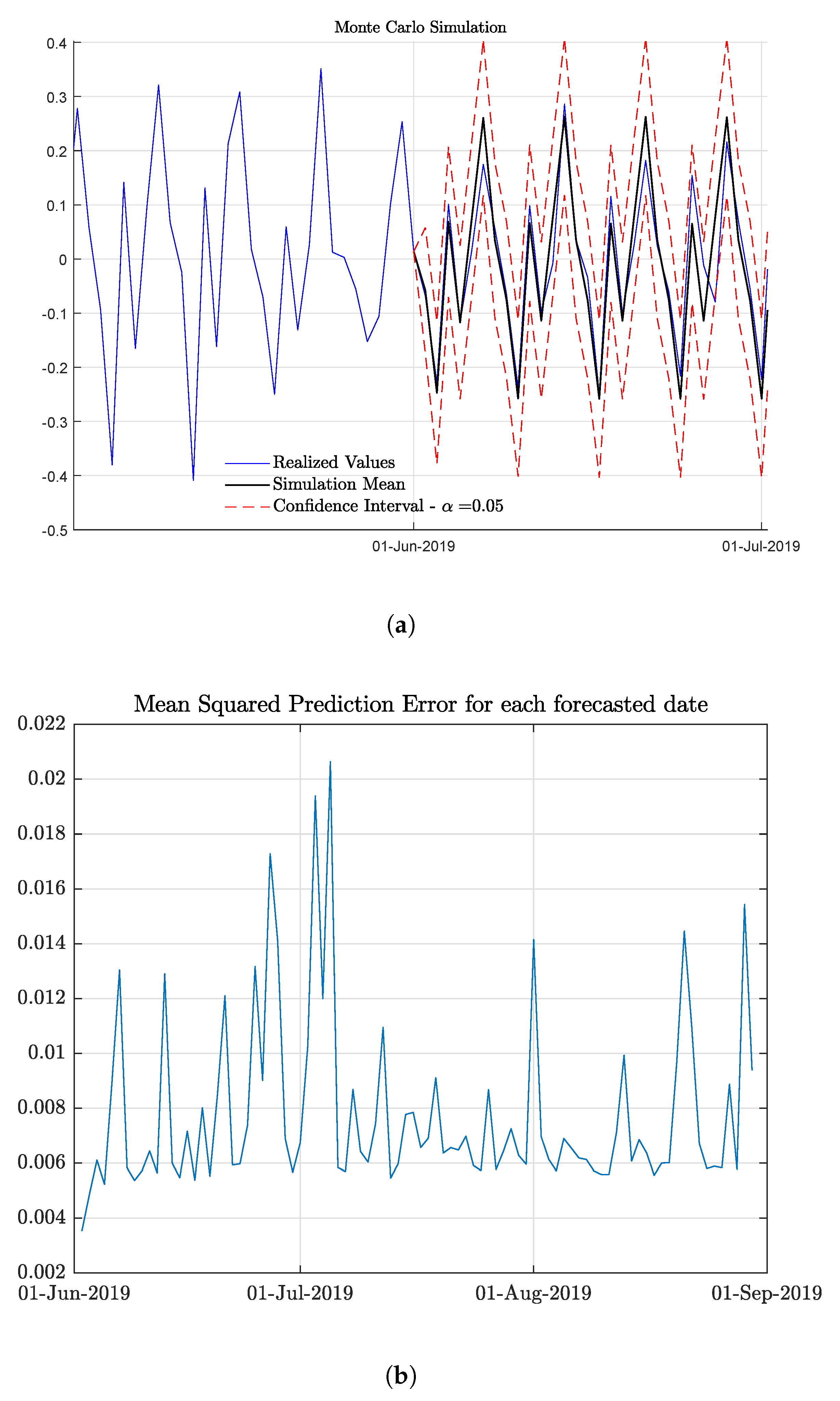
The NIG distributions have the best AIC values, supporting the hypothesis behind model innovations; the Kolmogorov–Smirnov test fails to reject the null-hypothesis that standardized residuals are drawn from the NIG distribution. Another validation test is related to the forecasting power of the model. In Figure 13 panel (a), we show forecasted trajectories for the next month (30 days) by considering ten thousand Monte Carlo (MC) simulations under the assumption of NIG distributed errors. Let ${\widehat{R}}_{t+j}^{\left(s\right)}$ be the forecasted value at $t+j$ under the s-th MC trajectory, and $MSP{E}_{t+j}:=\frac{1}{\mathrm{10,000}}{\sum }_{s=1}^{\mathrm{10,000}}{\left[{\widehat{R}}_{t+j}^{\left(s\right)}-R_{t+j}\right]}^2$ the mean squared prediction error of the whole set of simulated trajectories at $t+j$.

Figure 13, panel (b), shows the values of $MSP{E}_{t+j}$ with $t=$ 1-June-2019 for $j=1,\cdots ,92$ (the next three months). We have also considered the mean of MSPEs over the 3-month forecasting horizon $\overline{MSPE}:=\frac{1}{92}{\sum }_{t=1}^{92}\frac{1}{\mathrm{10,000}}{\sum }_{s=1}^{\mathrm{10,000}}{\left[{\widehat{R}}_{t+j}^{\left(s\right)}-R_{t+j}\right]}^2$. Model (7)–(8) achieved the lowest value $\overline{MSPE}=0.0116$ among all the models that we have tested, further validating the choice of parameters.

4. Option Pricing

4.1. Competition, Closures, and the Movie Theater

Considering to the contemporary media landscape, we note of course a relatively new but formidable media company whose distribution model significantly challenges theatrical exhibition: Netflix. Are investments built around the 100-plus-year-old theatrical-release industry formula (or the now almost fifty-year-old blockbuster model) even worth considering when Netflix is publicly traded? How, in the face of the streaming juggernaut(s) can we justify an index based on ROI determined by the domestic theatrical box office? Moreover, how—when all theaters were recently shuttered for the better part of a full year—can we argue for the value of theatrical box office in determining an index?

The “end of movie theaters” has long been proclaimed, yet they have—to this point at least—remained a viable part of our entertainment landscape and, moreover, a key player in the business model of motion picture monetization, as the history and summary of this industry has made clear. Like many brick-and-mortar retail spaces, the COVID-19 shutdown put an additional strain on these businesses, as consumers who were already increasingly looking to online order-and-delivery options were forced to do so in the face of closed storefronts, exacerbating the tenuous conditions of demand for such spaces. Unlike most retailers, however, movie theaters have always traded heavily in novelty and newness and, at least since the embrace of the blockbuster, built the bulk of their business on the uniqueness of the experience (hence the focus on “event” films). In addition, for the film industry, the circumstances of the shutdown affected exhibition and production equally and all films in the production pipeline were also stopped, so that the supply chain halted at the same time that access to retail did. This caused most of the major distributors to shift their theatrical release dates back to a later date (e.g., Paramount’s Top Gun: Maverick). As a result, the theater closures caused distributors to adjust and reallocate resources, but it is unlikely to result in the complete deprioritization of theatrical distribution all together since, as we have already demonstrated, the ROI model is so heavily weighted toward such a release pattern.13

Additionally, Netflix and other streaming services/OTT platforms are hardly the first new media technology to threaten the business practices and economic viability of American motion pictures, the film companies, or their collective exhibition practices. In the years following World War II, the explosion of television into American homes appeared to threaten the future of the film industry. Yet through a mix of technological shifts and business adaptations, motion pictures remained a thriving, viable, and often exciting aspect of America’s media environment. The rise of home video in the late 1970s and early 1980s was equally foreboding, yet Hollywood leveraged their product against the needs of cable programmers and reimagined home video sales to come out better economically in the mid-1980s than it had been a decade earlier Meehan (2008) and Landry and Greenwald (2018). Looking again at today’s OTT platforms in relation to the film companies, we can now recognize film studios such as Disney and Warner Bros. that are acquiring streaming services or opening their own as “following the historical industry pattern of letting others do the pioneering R&D work and then taking over the technologies” Landry and Greenwald (2018). From no less than PriceWaterhouseCoopers’ recent Global Entertainment and Media Outlook we also read: “Netflix and other streaming platforms are increasingly influential and continue to invest in original and feature-length content, but are still not considered to be competing directly with the Hollywood majors” PwC (2019). Like television and home video before, the COVID-related theater closures are likely to reconfigure but not eliminate the theatrical market; this is especially true for the blockbusters and event films that constitute such a significant portion of the American box office.

4.2. Dodd-Frank Goes to the Movies

Having argued for the construction of an index built, in the current media environment, on the ROI of the domestic box office, we turn to another potential deterrent, this time legal in nature. We proceed, nonetheless, on the premise that while laws may change, math endures.

Movies and onions form an unlikely pair just about anywhere; this is especially true under the jurisdiction of the United States Commodity Futures Trading Commission (CFTC). Yet it is these two—and these two alone—which are expressly excluded from the definition of “commodity” and thus restricted from futures contracts in the U.S. Onions were restricted in 1958 after Vincent Kosuga cornered the market to the detriment of American onion farmers Raviv (2018). That restriction stood, and stood alone, for 52 years until 2010 and the passing of the Dodd-Frank Wall Street Reform and Consumer Protection Act, designed predominantly to restrict behaviors viewed as responsible for the 2008 housing crisis. Yet, as happenstance would have it, at the same time the U.S. Congress was drafting that bill and negotiating what would and would not be included, Robert Swagger and Cantor Fitzgerald were separately seeking clearance from the CFTC for their motion picture box office futures (MDEX and Cantor Futures Exchange, respectively) which both—if somewhat differently—allowed investors to bet the futures of individual films produced and released theatrically in America. Though several smaller production companies such as Lionsgate significantly supported such a futures market Burns (2010), Hollywood’s major players got scared, to put it plainly, and sent their lobbyists (along with their media-conglomerate-backed funds) to Washington to find a way to scuttle this perceived threat Anderson (2011) and Graser (2010). Remarkably, Hollywood found a “solution” in the timing of the Dodd-Frank bill, which made a late addition that reads:

“Section 1a of the Commodity Exchange Act (7 U.S.C. 1a) is amended…by striking “except onions” and all that follows through the period at the end and inserting the following: “except onions (as provided by the first section of Public Law 85–839 (7 U.S.C. 13–1)) and motion picture box office receipts (or any index, measure, value, or data related to such receipts), and all services, rights, and interests (except motion picture box office receipts, or any index, measure, value or data related to such receipts) in which contracts for future delivery are presently or in the future dealt in”.” 111th Congress of the United States (2010).

So: onion and movies—or, more accurately: neither onions nor movies. This restriction on the market in relation to just these two commodities raises for us a perhaps obvious question: Is the ban a result of lobbying activities or is it a reasonable law that protects the market? This project revisits the idea of such a motion picture index. Rather than designing future contracts around individual titles and allowing investors and other market players to purchase (and perhaps, per Hollywood fearmongers, manipulate) these locally devised insurance policies, we have reimagined this on a significantly grander scale and at the level of the broader American film industry.

4.3. Developing Call and Put Options

In this section we construct a simple artificial option market on the daily movie index, where only European call and put options are traded. A European call option is a contract signed at a certain date t, which gives to the holder the right to buy the underlying asset, in this case the movie index I, at a fixed future date T and at a fixed price K. The option will be exercised only if the price at T of the underlying asset is greater than the strike price K. The pay-off of the holder at T will be then given by: $max\left(I_T-K,0\right)$. On the contrary, a put option gives the holder the right to sell the movie index; in this case the holder pay-off at T will be: $max\left(K-I_T,0\right).$ The two contracts have a price of say ${\mathsf{\Phi }}_c\left(t,T,K\right)$ and ${\mathsf{\Phi }}_p\left(t,T,K\right)$ respectively. We can think of these contracts as a type of insurance for an investor in the underlying asset and the two option prices as the premium of the insurance. If $K=I_t$ (the strike price and the price of the underlying asset at t are equal) we say that the option is at the money, if instead $K\gtrless I_t$, we say that the option is out the money or in the money respectively. The above relationship can be expressed by the ratio $\frac{I_t}{K}$, which is called moneyness; it describes the intrinsic value of an option in its current state.

The goal of the rest of this section is to compute the set of prices of an option contract written on the movie index, for different values of the strike price K and the time to maturity T. In other words, we would like to price an insurance on the index I. Suppose that at date t the index is priced $I_t$ and that we want to price the two European options with time to maturity $T>0$. We first fit the model (7)–(8) with NIG standardized residuals and then simulate S trajectories of the return series $R_t$ over the period $\left[t,T\right]$ by means of Monte Carlo (MC) techniques. In this way we obtain a fan of S forecasted index return values ${\left\{{\widehat{R}}_{s,\tau }\right\}}_{\tau =t}^T$ for $s=1,\cdots ,S$, where to each trajectory s is associated the probability $p_s=\frac{1}{S}$. The set of these probabilities defines the discrete probability measure $\mathbb{P}$ associated with the index return. We can then define the forecasted index price at T in the s trajectory as ${\widehat{I}}_{s,T}=I_0{\prod }_{\tau =t}^T\left(1+{\widehat{R}}_{s,\tau }\right).$

In order to price the call and put options, we refer now to the fundamental theorem of asset pricing: the price of a contract is equal to the discounted expected value under a risk neutral measure of the contract pay-off, see for instance Delbaen and Schachermayer (1994). The discount is computed with respect to a risk free interest rate $rf\left(t,T\right)$ between t and T, which in this work has been set equal to the treasury bill with maturity $\left(T-t\right)$. The risk neutral measure is a probability measure $\mathbb{Q}$, equivalent to the real measure $\mathbb{P}$, and such that the expected value, conditioned to the filtration ${\mathcal{F}}_t$, of the discounted price at T of the underlying asset is equal to its price at t:

$$I_t={\mathbb{E}}^Q\left[I_T{e}^{-rf\left(t,T\right)}|{\mathcal{F}}_t\right].$$

(9)

Formula (9) can be equivalently stated in terms of returns:

$$1={\mathbb{E}}^Q\left[R_T{e}^{-rf\left(t,T\right)}|{\mathcal{F}}_t\right].$$

(10)

Given the risk neutral probability measure $\mathbb{Q}$, European option prices on the index I can be computed as:

$${\mathsf{\Phi }}_c\left(t,T,K\right):={\mathbb{E}}^Q\left[max\left(I_T-K,0\right)e^{-rf\left(t,T\right)}|{\mathcal{F}}_t\right],$$

(11)

$${\mathsf{\Phi }}_p\left(t,T,K\right):={\mathbb{E}}^Q\left[max\left(K-I_T,0\right)e^{-rrf\left(t,T\right)}|{\mathcal{F}}_t\right].$$

(12)

In the discrete setting of this paper, we have that ${\mathbb{E}}^P\left[R_T{e}^{-rf\left(t,T\right)}|{\mathcal{F}}_t\right]={\sum }_{s=1}^S{p}_s{\widehat{R}}_T{e}^{-rf\left(t,T\right)}$, and the option price problem is essentially reduced to finding $\mathbb{Q}$. We have followed the approach of minimising the Kullback–Leibler divergence between $\mathbb{Q}$ and $\mathbb{P}$ as described in Avellaneda et al. (2001), such that it can be stated as the convex problem defined as follows:

$$\begin{array}{cc}\hfill & \underset{q_s,s=1,\cdots ,S}{min}\sum _s^S{q}_{s}ln\frac{q_s}{p_s}\hfill \\ \hfill & \mathrm{such}\mathrm{that}:\hfill \end{array}$$

(13)

$$\begin{array}{cc}\hfill & \sum _{s=1}^S{q}_s=1\hfill \end{array}$$

(14)

$$\begin{array}{cc}\hfill & \sum _{s=1}^S{\widehat{R}}_T{q}_s{e}^{rf\left(t,T\right)}=1\hfill \end{array}$$

(15)

$$\begin{array}{cc}\hfill & 0<q_s\le 1,s=1,\cdots ,S\hfill \end{array}$$

(16)

Once we have found the measure $\mathbb{Q}$, we can compute option prices by means of the two simple formulas:

$${\mathsf{\Phi }}_c\left(t,T,K\right):=\sum _{s=1}^S{q}_s\left[max\left({\widehat{I}}_{s,T}-K,0\right)e^{-rf\left(t,T\right)}\right],$$

(17)

$${\mathsf{\Phi }}_p\left(t,T,K\right):=\sum _{s=1}^S{q}_s\left[max\left(K-{\widehat{I}}_{s,T},0\right)e^{-rf\left(t,T\right)}\right].$$

(18)

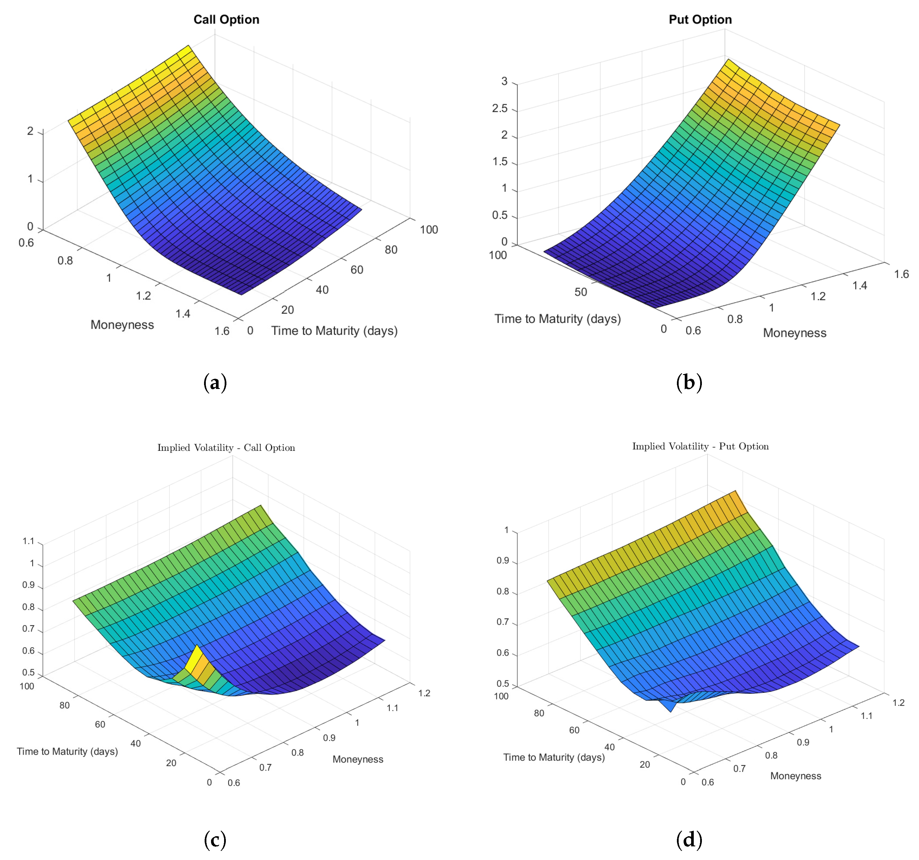
We now suppose a price option contract signed on Saturday, 1 June 2019, when the movie index price I is equal to 5.0631. We run the option pricing model described above for maturity values T in the set $\left\{t+7,t+14,\cdots ,t+98\right\}$, or once a week for approximately three months, and for strike prices in the interval $\left[I_0-2,I_0+2.5\right]$. We express in Figure 14 the surface representing call, panel (a), and put, panel (b), option prices for every combination $(\frac{I_t}{K},T)$. As expected, call and put prices increase with T, as we face a higher uncertainty on the future index price value; the price of the call increases (decreases) as the moneyness decreases (increases).

Finally, we would like to check the implied volatility surface of this artificial option market constructed on the index price I. Given the prices obtained by formulas (17)–(18) for a given couple $(K,T)$, it is possible to obtain the value of the volatility parameters ${\sigma }_c^{*}$ and ${\sigma }_p^{*}$ in the usual Black-Scholes-Merton formula so that it produces the same option prices for the call and for the put respectively. It is then possible to draw the surface ${\sigma }_c^{*}\left(\frac{I_t}{K},T\right)$ and ${\sigma }_p^{*}\left(\frac{I_t}{K},T\right)$: see panels (c)–(d) in Figure 14.

5. Movie Index and the Stock Market

5.1. The Basic Economics of Hollywood—Part II

The classic Hollywood studios started as private companies. They were run as such from their origins in the 1910s and 1920s through the period known as Classical Hollywood—which was both an industrial and stylistic description Bordwell et al. (1985)—into the 1960s when the pressures associated with losing their exhibition chains and dropping audience numbers forced most to sell to conglomerates (some private, some public).14 The flush of money around home video in the early 1980s convinced a number of start-up film production companies to go public, but the ultimate losses suffered by their investors and the difficulty in launching unknown companies has generally prevented any similar situation from arising again Vogel (2014). In our current media environment, almost all of the large film companies are part of a larger media conglomerate and those smaller ones that stand alone are usually private and not publicly traded.15

Only four companies that engage in film production are currently included on the S&P 500 and none can truly claim to be film companies primarily: Comcast (CCZ), whose principal business is telecommunications, owns Universal Pictures and DreamWorks Animation; AT&T (T), another telecommunications giant, owns Warner Bros.; Viacom—now ViacomCBS (VIAC)—is a media conglomerate focused on content creation whose subsidiary companies include Paramount Pictures; and Disney (DIS), which owns Walt Disney Pictures as well as Marvel, LucasFilm, Pixar, Fox, and others film subsidiaries, but also theme parks, television, the DisneyPlus streaming service, and loads of IPs (intellectual property) that it monetizes through extensive merchandising.16 Netflix (NFLX), Amazon (AMZN), Apple (AAPL), and other similar companies can also be found on the S&P 500, and they are increasingly moving into content production—including films that occasionally release to theaters—but their production is wholly geared toward driving their subscription service and thus operates predominantly under a different business model measured primarily in terms of subscribers. Only a few other companies produce and distribute enough films to warrant discussion in terms of the broad dynamics of the field. Sony Pictures, which owns Columbia Pictures, is operated as a subsidiary of Sony Entertainment, which is itself a part of the multinational technology and media conglomerate Sony Corp. (SNE) and listed on the NYSE; AMC Networks (AMCX), which owns IFC Films, is included in the S&P 400.17 This nesting of movie and entertainment content producers in larger national or multinational media or telecommunication conglomerates then is clearly the rule and not the exception.

5.2. Analysis of Index–Stock Market Dependence

In the remainder of this paper, we investigate possible dependence relationships between our movie index and the U.S. stock market. We consider public companies operating in sectors connected with the American film industry: production, distribution, and theater ownership. We indeed argue that a particular positive box office earnings could lead to an increase in the production/distribution company stock demand. Similarly, positive and high box office earnings could increase fundamental values expectations for the movie theater industry, with again, a consequent increase in stock demand.

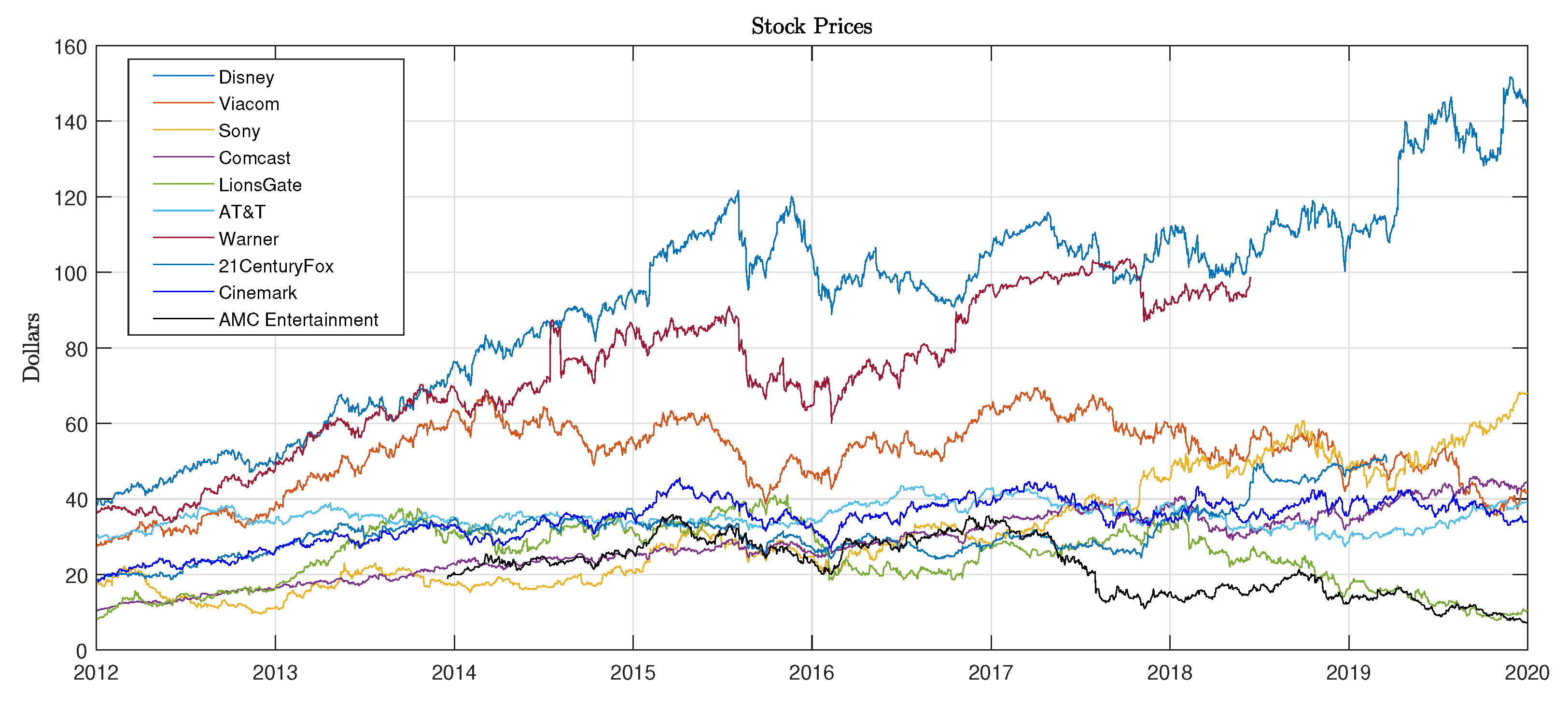
We have mentioned that the production/distribution movie market is mainly driven (in 2021) by eight public companies quoted in U.S. stock markets. Six of these are producer/distributors; the major players we consider here are DIS (Disney), VIAC (ViacomCBS), SNE (Sony), CCZ (Comcast), LGF (Lionsgate), and T (AT&T). The range of corporate scale and business interests varies widely across these, from huge media and telecommunications companies such as Comcast and AT&T, to Disney and its empire built on its intellectual properties, to Lionsgate which focuses heavily on film production and distribution. Likewise, theaters in the U.S. are predominantly controlled by three public companies: Cinemark Holdings Inc (CNK), AMC Entertainment Holdings, Inc. (AMC), and Regal Entertainment Group (RGC); we only consider here the first two, as Regal is now owned (since February 2018) by the UK theater chain Cineworld. In Figure 15 we illustrate price dynamics for the ten companies (now reduced to eight) spanning the period 3 January 2012–31 December 2019.

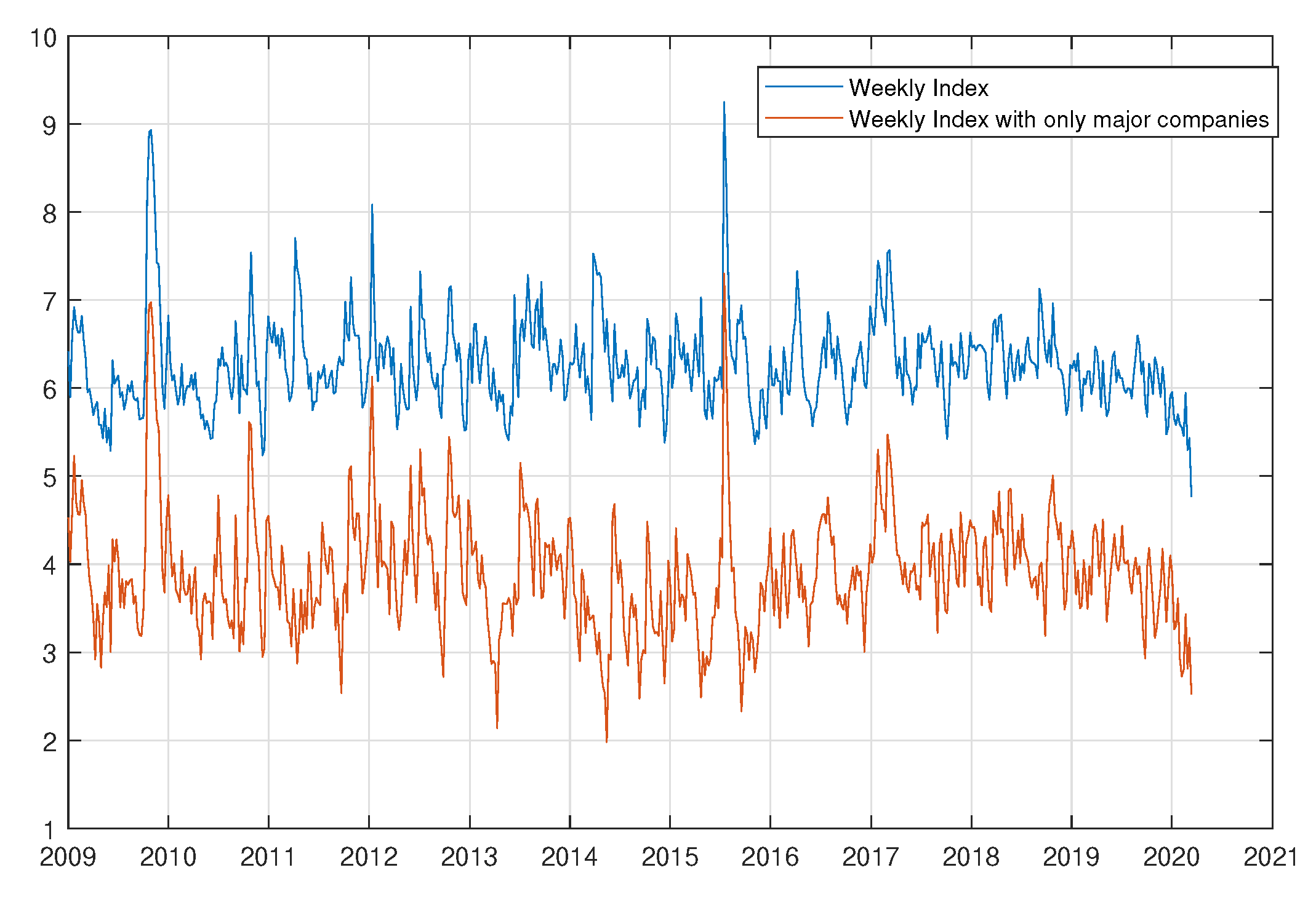
A potential problem in detecting dependencies arises from time steps associated with stock price series and our movie index I: stock markets are closed during the weekend, while the movie index records data for every calendar day. In order to overcome this issue, we consider in this section a weekly equivalent $I_w$ of the movie index; its dynamic is depicted in Figure 16, along with the weekly movie index constructed by just considering movies released by the eight (now six) major public film production/distribution companies.

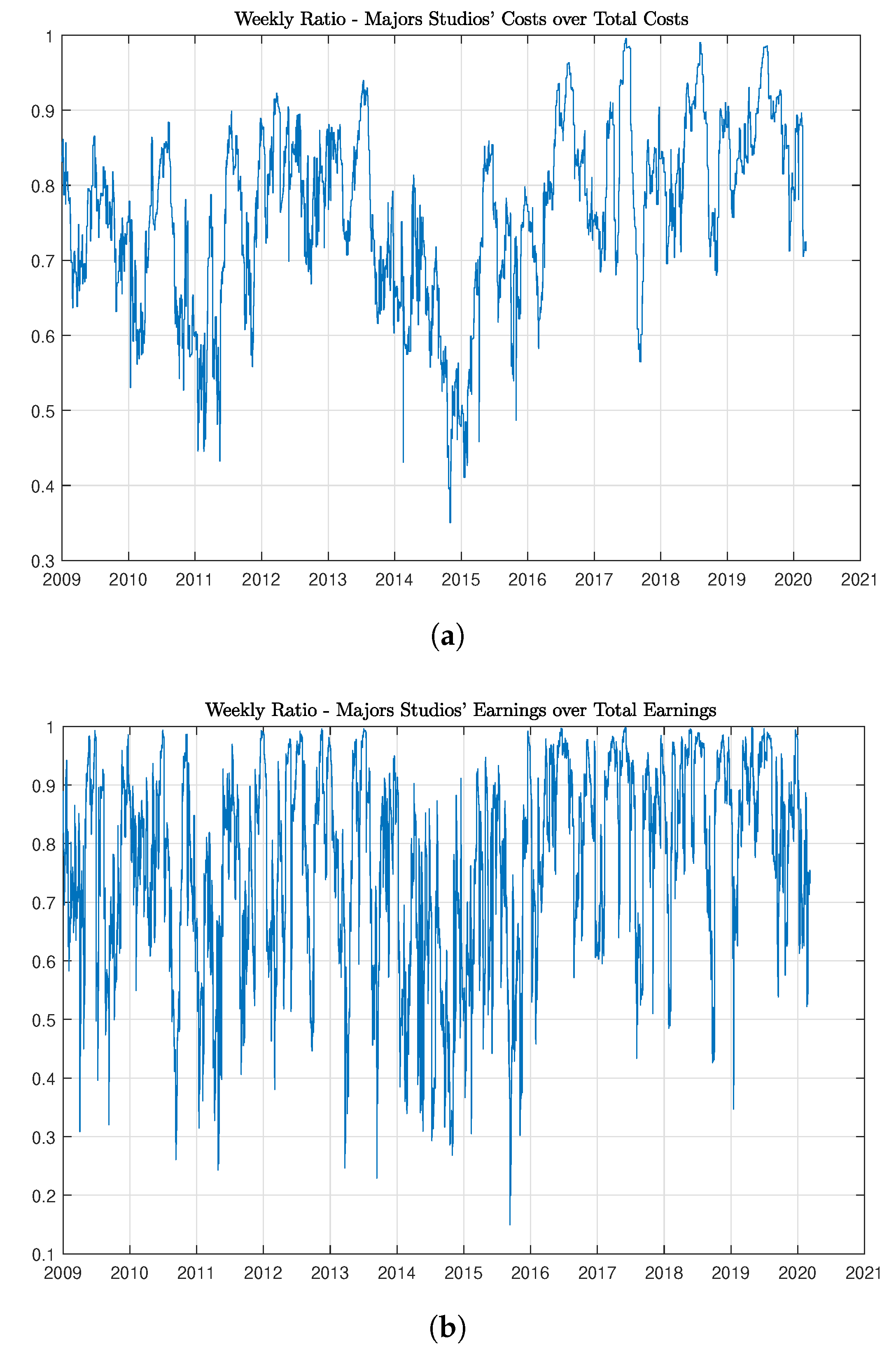
In Figure 17 we have plotted two ratios: the former is the ratio of daily box office costs related to movies produced or distributed by the public companies mentioned above over the total value of daily production costs $c_t$; the latter is the ratio of daily box office earnings related to movies produced or distributed by the public companies over the total value of daily box office earnings $y_t.$ We then construct a weekly stock price index based on the public companies addressed above in order to compare stock prices and the box-office returns. Since companies take part in the movie industry with different loads, which also vary with time, the logistics of constructing the stock price index is neither trivial nor straightforward, as it is difficult and often impossible to find movie-specific expenditures in company balance sheets. This is due, in part, to the long period of investment for individual films that typically includes preproduction and, for distributors, marketing costs as well. In order to approximate the movie market share of a company during a particular week, we can take several approaches such as focusing on the number of movies distributed or on the ratio of total weekly costs. In what follows we present a sequence of attempts—from the simplest to the more complex—to find a stock price index which exhibits causal relationships with the weekly movie index.

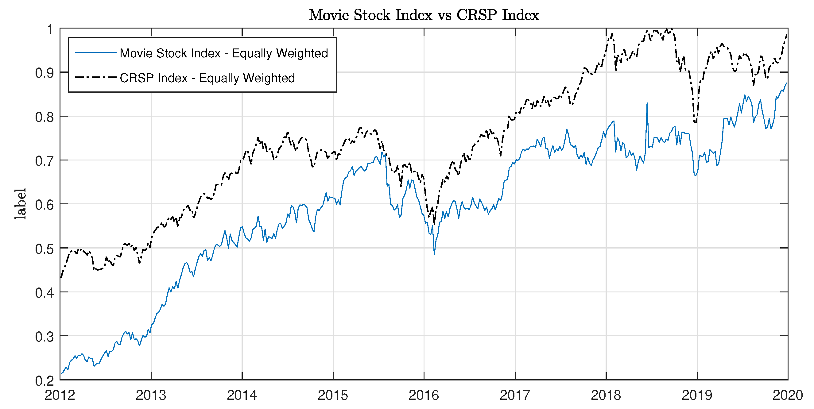
The first attempt was realized by constructing an equally weighted weekly index $S_1$ of production/distribution companies’ stock prices. Values, normalized in the interval $[0,1]$, of this Movie Stock Index are shown in Figure 18, along with values of the Equally Weighted CRSP Index; main statistics are reported in

Table A4. Variables—Univariate Statistics.

Variable	Mean	Std	Skewness	Kurtosis	${\mathbf{CVaR}}_{0.05}^{\left(\mathit{l}\right)}$	${\mathbf{CVaR}}_{0.95}^{\left(\mathit{u}\right)}$
Equally weighted Stock Index $S_1$	0.003	0.024	−1.383	6.600	−1.055	0.051
Equally weighted Stock Index $S_2$	0.001	0.036	−1.745	7.390	−1.081	0.072
Equally weighted Stock Index $S_3$	0.004	0.099	0.037	5.750	−1.223	0.239
Equally weighted CRSP Index	0.002	0.018	−1.296	4.752	−1.039	0.039
Weekly Movie Index	−1.0001	0.0613	1.680	10.426	−1.100	0.164
Stock index innovations $h_1$	−1.014	1.014	0.614	10.105	−1.260	2.280
Stock index innovations $h_2$	−1.0220	1.031	−1.113	11.145	−1.3960	2.0240
Stock index innovations $h_3$	0.0060	0.906	−1.036	6.413	−1.104	2.1830
Movie index innovations $h_M$	0.116	1.058	2.506	18.445	−1.395	3.078

. Of course we observe that the movie stock index is strongly influenced by the overall economics/market condition, represented here by the equally weighted CRSP Index.

In order to filter overall market dynamics, we regress stock index returns $r_{1,t}$ on CRSP Index returns $r_t^{\left(crsp\right)}$, namely we find $\beta$ in $r_{1,t}=\beta ·r_t^{\left(crsp\right)}+e_{1,t}$. The fitted $\widehat{\beta }$ is equal to $0.885$, with a p-value of the F-statistic equal to zero, proving a deep connection between stocks in our index and the whole U.S. stock market. The resulting series of residuals $\left\{e_{1,t}\right\}$ has been filtered through an ARIMA(1,0,0)-GARCH(1,1) autoregression model,18 producing a series of innovations (standardised residuals) $h_1$. Analogously, an ARIMA(1,1,1)-GARCH(1,1) model has been fitted on the weekly movie index $I_w$, with a resulting series of innovations $h_m$.

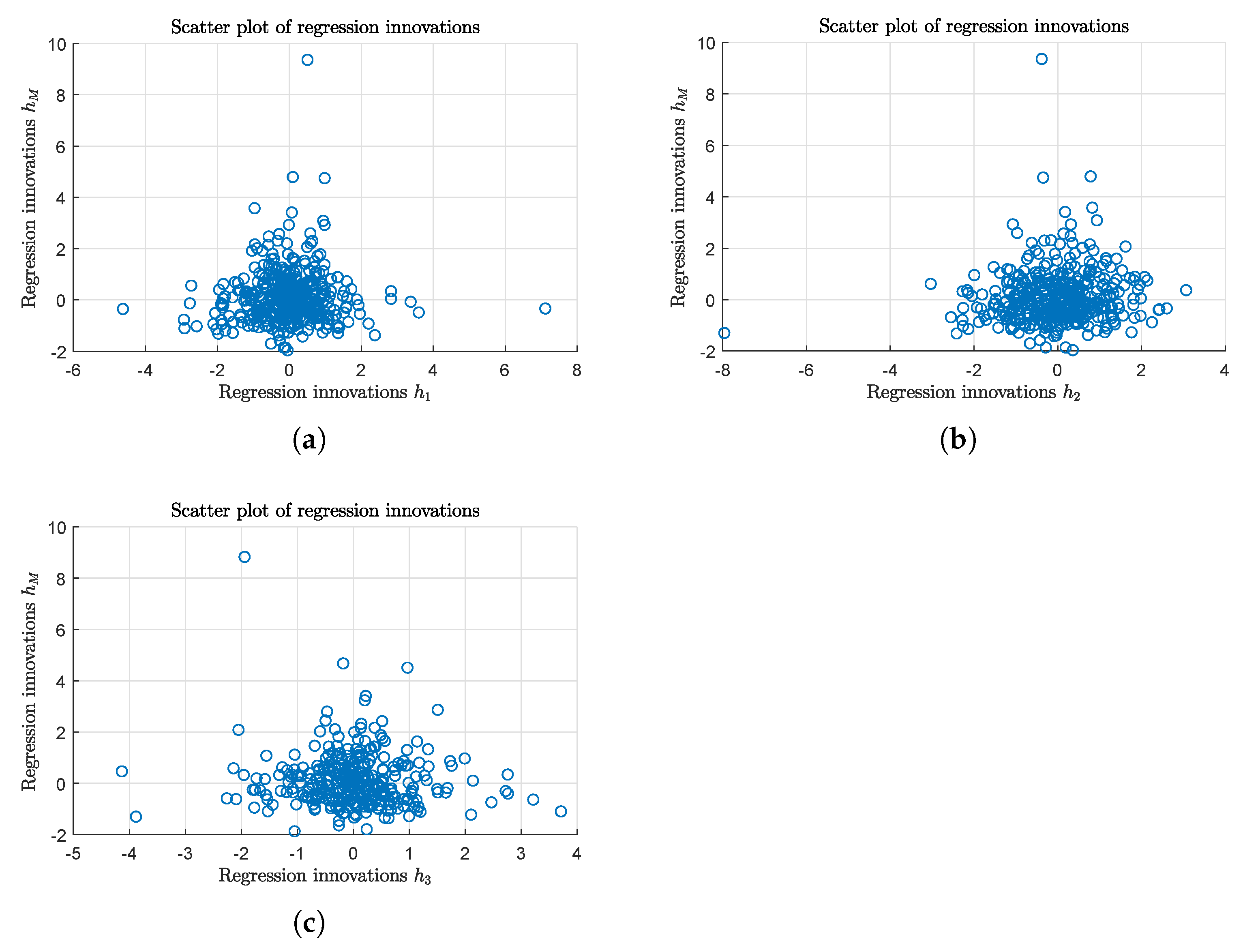
We then couple the two series to form the bivariate sample vector $[h_1,h_m]$, which is then used to check dependencies between the weekly movie index $I_w$ and the stock movie index $S_1$. The sample scatter plot of $[h_1,h_m]$ is depicted in panel (a) of Figure 19, and in Table A4 we show univariate statistics for the two series of innovations. In order to check concordance dependency, we fit the empirical beta copula to the bivariate sample and then we compute its Kendall’s tau and Spearman’s rho. The Linear Correlation coefficient and the two rank concordance measures, Kendall’s tau and Spearman’s rho, stored in

Table A6. Dependency measures between the two vectors of innovations.

Bivariate Sample	Linear Correlation	Kendall’s tau	Spearman’s rho
$[h_M,h_1]$	0.0397	0.0112	0.0190
$[h_M,h_2]$	0.0994	0.0728	0.1088
$[h_M,h_3]$	−1.0500	−1.0290	−1.0463

, are all closed to zero, suggesting a possible case of independence.

We also investigated possible dependency structures in the lower-left and upper-right quadrant of the joint empirical bivariate distribution of $[h_1,h_m]$. This analysis has been performed by means of two quantities, the so-called CoVaR and CoES (also called CoCVaR), presented in Girardi and Ergun (2013) and Huang and Uryasev (2018) respectively.19 The lower-left quadrant ${\mathrm{CoVaR}}_{\alpha ,\beta }^{\left(l\right)}\left(Y\right|X)$ between two random variables X and Y is defined as the $\beta$-quantile of the conditional probability $P\left(Y\right|X\le {\mathrm{VaR}}_{\alpha }\left(X\right))$, where ${\mathrm{VaR}}_{\alpha }\left(X\right)$ is the $\alpha$-quantile of the distribution of X. The upper-right quadrant ${\mathrm{CoVaR}}_{\alpha ,\beta }^{\left(u\right)}\left(Y\right|X)$ between two random variables X and Y is defined as the $\beta$-quantile of the conditional probability $P\left(Y\right|X\ge {\mathrm{VaR}}_{\alpha }\left(X\right))$. The CoES is defined instead as:

$$\begin{array}{cc}\hfill & {\mathrm{CoES}}_{\alpha ,\beta }^{\left(l\right)}\left(Y\right|X)=\frac{1}{\beta }{\int }_0^{\beta }{\mathrm{CoVaR}}_{\alpha ,t}^{\left(l\right)}\left(Y\right|X)dt\hfill \end{array}$$

(19)

$$\begin{array}{cc}\hfill & {\mathrm{CoES}}_{\alpha ,\beta }^{\left(u\right)}\left(Y\right|X)=\frac{1}{1-\beta }{\int }_{\beta }^1{\mathrm{CoVaR}}_{\alpha ,t}^{\left(u\right)}\left(Y\right|X)dt\hfill \end{array}$$

(20)

In

Table A7. CoVaR and CoES measures between the two vectors of innovations.

Conditional Sample	${\mathbf{VaR}}_{0.05}^{\left(\mathit{l}\right)}$	${\mathbf{CoVaR}}_{0.05}^{\left(\mathit{l}\right)}$	${\mathbf{CoES}}_{0.05}^{\left(\mathit{l}\right)}$	${\mathbf{VaR}}_{0.95}^{\left(\mathit{u}\right)}$	${\mathbf{CoVaR}}_{0.95}^{\left(\mathit{u}\right)}$	${\mathbf{CoES}}_{0.95}^{\left(\mathit{u}\right)}$
$\left(h_1\right|h_M)$	−1.7810	−1.9754	−1.0235	1.9135	0.9797	0.9827
$\left(h_M\right|h_1)$	−1.1149	−1.1418	−1.3146	1.3555	0.4230	0.7211
$\left(h_2\right|h_M)$	−1.5432	−1.4171	−1.9092	1.5619	1.6186	1.6118
$\left(h_M\right|h_2)$	−1.1149	−1.2971	−1.3161	1.9135	2.0621	2.0505
$\left(h_3\right|h_M)$	−1.5267	−1.2208	−1.2208	1.4212	1.7476	1.7476
$\left(h_M\right|h_3)$	−1.1149	−1.2995	−1.2995	1.9135	2.8661	2.8661

we show results obtained by setting $\alpha =\beta =0.05$ for left-lower quadrant dependency and $\alpha =\beta =0.95$ for upper-right dependency. It is easy to prove that if two random variables X and Y are independent, then $\mathrm{VaR}\left(\mathrm{Y}\right)=\mathrm{CVaR}\left(Y\right|X)$.20 As such, we can test tail dependence between the two series of innovation by comparing VaR and CoVaR values, for instance by looking at the ratio

$${\chi }^l\left(h_1\right|h_M):=\frac{{\mathrm{CoVaR}}_{0.05,0.05}^{\left(l\right)}\left(h_1\right|h_M)}{{\mathrm{VaR}}_{0.05}^{\left(l\right)}\left(h_1\right)},$$

(21)

which in the independence case will be equal to one; values greater than one will instead indicate positive left-lower tail dependence. The value of ${\chi }^l\left(h_1\right|h_M)=\frac{-1.9754}{-1.7810}=1.1092$ is higher than one, suggesting a possible, albeit low, left-lower tail dependency. The lack of evidence suggesting a strong dependency structure between the weekly movie index and stock index $S_1$ in the previous analysis21 could be the result of a wrong choice of the stock index; this can be due to the wrong choice of stocks and/or by the wrong choice of index weights. In light of these considerations we have tried the following variations, taken one at a time, to the previous machinery:

• We consider the stock index $S_2$ composed only by the two major U.S. companies which own movie theaters. In this case the $R^2$ statistic of the regression on the CRSP index is lower than the value found before, suggesting a lower dependency of this index with general market conditions; however, we can observe that the ratio

  $${\chi }^l\left(h_2\right|h_M)=\frac{-2.4171}{-1.5432}=1.5663$$

  is greater than the previous case. This could be a signal of a stronger left-lower tail dependency.
• We alter the weight in the stock index formed by production/distribution companies $S_1$: the weight assigned to a particular company is the proportion of the total weekly cost $c_t$ held by that company over the total cost for for the entire industry for that same week. We call $S_3$ the resulting stock index. In this case we lost the dependency of the stock index with the overall U.S. financial market with a very low value of $\beta$ and a $R^2$ statistic close to zero. However, the dependence structure between the two innovations series $h_3$ and $h_m$ appear to be more complex: correlation and concordance measure reveal a negative sign, suggesting a countermonotone relationship, whereas both lower-left and upper-right dependence measures appear to be positive.

All of the analyses performed in this section suggest the lack of a clear global dependency between the weekly movie index and the U.S. stock market; this confirms expectations and expands results from previous studies Ravid (1999) and Elberse (2007). Indeed, potential investors could not hedge the risk by trading the quoted stocks either directly or through derivatives contracts related to the prominent industry players. The lack of dependency structures between the movie index and the proposed stock market indices reinforces the potential usefulness of the movie index to provide a benchmark for pricing insurance products.

6. Conclusions

In this work we propose a daily index that represents the daily return at the box office of the American film industry. Current government regulation in the U.S. forbids the trading of any derivative securities written on products related to the domestic movie industry. This ban is nevertheless criticized by certain producers, particularly those operating outside the dominant production companies, who look for insurance products able to hedge the significant investment risk associated with film production. We provide quantitative analyses supporting the feasibility of pricing derivative contracts on the movie index by means of time-discrete option pricing methods. This result could be used to define and test insurance products, in the form of option contracts, and provide quantitative foundations to challenge the current restrictive statutes and assess whether, in such a market for film industry futures, Hollywood’s caution or the optimism of other players like Lionsgate is deemed the more prudent, economically beneficial direction. Moreover, such a futures market could be put into place in other countries with robust film industries, though certainly the volume and nature of such would require further evaluation. This work should then be regarded as a first building block for a more extensive quantitative analysis. Future research will focus on the definition of specific derivative contracts and the analysis, by means of simulations and back testing, of their potential effect on the domestic movie industry in America. This will require a more structured approach to decide whether or not a derivative market could be a hazard or a boon for the stability and efficiency of this industry.

References

- 111th Congress of the United States. 2010. Dodd-Frank Wall Street Reform and Consumer Protection Act of 2010. Washington, DC: Government Publishing Office, pp. 1376–2223. [Google Scholar]
- Anderson, Paul G. 2011. Back to the future[s]: A critical look at the film futures ban. Cardozo Arts & Entertainment Law Journal 29: 179–214. [Google Scholar]
- Angeli, Michael. 1991. Film; My Name Is Bond. Completion Bond. New York Times, August 11. [Google Scholar]
- Avellaneda, Marco, Robert Buff, Craig Friedman, Nicolas Grandechamp, Lukasz Kruck, and Joshua Newman. 2001. Weighted Monte Carlo: A new technique for calibrating asset-pricing models. International Journal of Theoretical and Applied Finance 4: 91–119. [Google Scholar] [CrossRef]
- Barndorff-Nielsen, Ole E. 1977. Exponentially decreasing distributions for the logarithm of particle size. Proceedings of The Royal Society A: Mathematical, Physical and Engineering Sciences 353: 401–19. [Google Scholar]
- Barndorff-Nielsen, Ole E. 1997a. Normal inverse Gaussian distributions and stochastic volatility modelling. Scandinavian Journal of Statistics 24: 1–13. [Google Scholar] [CrossRef]
- Barndorff-Nielsen, Ole E. 1997b. Processes of normal inverse Gaussian type. Finance and Stochastics 2: 41–68. [Google Scholar] [CrossRef]
- Bordwell, David, Janet Staiger, and Kristin Thompson. 1985. The Classical Hollywood Cinema: Film Style & Mode of Production to 1960. New York: Columbia University Press. [Google Scholar]
- Boyle, Charles. 2001. Hollywood and the insurance industry. Insurance Journal. September 17. Available online: https://www.insurancejournal.com/magazines/mag-features/2001/09/17/18502.htm (accessed on 19 April 2021).
- Burns, Michael. 2010. Letter to House Committee on Agriculture. Available online: https://www.cftc.gov/sites/default/files/stellent/groups/public/@otherif/documents/ifdocs/mburnshousecomitteeag041610.pdf (accessed on 19 April 2021).
- Caves, Richard. 2000. Creative Industries: Contracts between Art and Commerce. Cambridge: Harvard University Press. [Google Scholar]
- De Vany, Arthur. 2004. Hollywood Economics: How Extreme Uncertainty Shapes the Film Industry. London: Routledge. [Google Scholar]
- De Vany, Arthur, and W. David Walls. 2002. Does hollywood make too many R-rated movies? risk, stochastic dominance, and the illusion of expectation. Journal of Business 75: 425–51. [Google Scholar] [CrossRef]
- De Vany, Arthur, and W. David Walls. 2004. Motion picture profit, the stable Paretian hypothesis, and the curse of the superstar. Journal of Economic Dynamics and Control 28: 1035–57. [Google Scholar] [CrossRef]
- Dekom, Peter J. 2017. Movies, money and madness. In The Movie Business Book, 4th ed. Edited by Jason E. Squire. London: Routledge, pp. 99–115. [Google Scholar]
- Delbaen, Freddy, and Walter Schachermayer. 1994. A general version of the fundamental theorem of asset pricing. Mathematische Annalen 300: 463–520. [Google Scholar] [CrossRef]
- Eberlein, Ernst, and Ulrich Keller. 1995. Hyperbolic distributions in finance. Bernoulli 1: 281–99. [Google Scholar] [CrossRef]
- Elberse, Anita. 2007. The power of stars: Do star actors drive the success of movies? Journal of Marketing 71: 102–20. [Google Scholar] [CrossRef]
- Filson, Darren, David Switzer, and Portia Besocke. 2005. At the movies: The economics of exhibition contracts. Economic Inquiry 43: 354–69. [Google Scholar] [CrossRef]
- Girardi, Giulio, and A. Tolga Ergun. 2013. Systemic risk measurement: Multivariate garch estimation of coVaR. Journal of Banking & Finance 37: 3169–80. [Google Scholar]
- Graser, Marc. 2010. Basic instincts: Pic futures reward biz savvy. Variety 418: 25. [Google Scholar]
- Hall, Sheldon, and Steve Neale. 2010. Epics, Spectacles, and Blockbusters: A Hollywood History. Detroit: Wayne State University Press. [Google Scholar]
- Huang, Wei-Qiang, and Stanislav P. Uryasev. 2018. The CoCVaR approach: Systemic risk contribution measurement. Journal of Risk 20: 4. [Google Scholar] [CrossRef] [Green Version]
- Hylleberg, Svend, Robert Engle, Clive Granger, and Byung Sam Yoo. 1990. Seasonal integration and cointegration. Journal of Econometrics 44: 215–38. [Google Scholar] [CrossRef]
- King, Geoff. 2002. New Hollywood Cinema: An Introduction. London: I.B. Tauris Publishers. [Google Scholar]
- Kwiatkowski, Denis, Peter Phillips, Peter Schmidt, and Yongcheol Shin. 1992. Testing the null hypothesis of stationarity against the alternative of a unit root: How sure are we that economic time series have a unit root? Journal of Econometrics 54: 159–78. [Google Scholar] [CrossRef]
- Landry, Paula, and Stephen R. Greenwald. 2018. The Business of Film: A Practical Introduction. Boca Raton: CRC Press. [Google Scholar]
- Madan, Dilip B., and Eugene Seneta. 1990. The variance gamma (v.g.) model for share market returns. Journal of Business 63: 511–24. [Google Scholar] [CrossRef]
- Mainik, Georg, and Eric Schaanning. 2014. On dependence consistency of covar and some other systemic risk measures. Statistics & Risk Modeling 31: 49–77. [Google Scholar]
- Masters, Kim. 2014. ’Fast & Furious 7’ Insurance Claim Could Reach Record-Breaking $50 Million. Hollywood Reporter, May 21. [Google Scholar]
- Meehan, Eileen R. 2008. Ancillary markets—Television: From challenge to safe haven. In The Contemporary Hollywood Film Industry. Edited by Peter McDonald and Janet Wasko. Oxford: Blackwell Publishing, pp. 106–19. [Google Scholar]
- Molla, Rani, and Peter Kafka. 2021. Here’s Who Owns Everything in Big Media Today. Vox, January 11. [Google Scholar]
- Phillips, Richard. 2004. The global export of risk: Finance and the film business. Competition & Change 8: 105–36. [Google Scholar]
- PwC. 2019. PriceWaterhouseCoopers 2019–2023 Global Entertainment and Media Outlook. London: PwC. [Google Scholar]
- Ravid, S. Abraham. 1999. Information, blockbusters, and stars: A study of the film industry. Journal of Business 72: 463–92. [Google Scholar] [CrossRef] [Green Version]
- Raviv, Shaun. 2018. Box Office Bomb: The Short Life of Popcorn Prediction Markets. The Ringer, November 15. [Google Scholar]
- Rockafellar, R. Tyrrell, and Stanislav Uryasev. 2000. Optimization of conditional value-at-risk. Journal of risk 2: 21–42. [Google Scholar] [CrossRef] [Green Version]
- Schatz, Tom. 2008. The studio system and conglomerate Hollywood. In The Contemporary Hollywood Film Industry. Edited by Peter McDonald and Janet Wasko. Oxford: Blackwell Publishing, pp. 3–42. [Google Scholar]
- Sedgwick, John. 2002. Product differentiation at the movies: Hollywood, 1946 to 1965. Journal of Economic History 62: 676–705. [Google Scholar] [CrossRef]
- Simonton, Dean Keith. 2009. Cinematic success criteria and their predictors: The art and business of the film industry. Psychology & Marketing 26: 400–20. [Google Scholar]
- TheNumbers. 2020. Movie Theatrical Daily Box Office Chart Archive. Beverly Hills: TheNumbers. [Google Scholar]
- Vogel, Harold L. 2014. Entertainment Industry Economics: A Guide for Financial Analysis, 9th ed. Cambridge: Cambridge University Press. [Google Scholar]
- Walls, W. David. 2005. Modeling movie success when ‘nobody knows anything’: Conditional stable-distribution analysis of film returns. Journal of Cultural Economics 29: 177–90. [Google Scholar] [CrossRef]
- Wyatt, Justin. 2015. High Concept: Movies and Marketing in Hollywood. Austin: University of Texas Press. [Google Scholar]
Figure 1.
(a) Total cost, (b) Total earnings, and (c) Return on investment for each movie in the data set, ordered with respect to the date of release.
Figure 2.
Histograms of C and Y, panels (a,b), and histogram of for the three partitions, panels (c–e).
Figure 3.
Logarithm of the ratio .
Figure 4.
Density estimation of , panel (a–c), and its tails, panels (b,c).
Figure 5.
Top-left panel (a) shows the number of daily data for each movie in the data set. Labeled points highlight movies with a number of daily data above the quantile. Bottom-left panel (c) shows the number of movies at each date t. In right panels (b,d) we see the corresponding histograms. 1—The Polar Express (2004) 2—The Hangover (2009) 3—Avatar (2009) 4—Winter’s Bone (2010) 5—Despicable Me (2010) 6—The King’s Speech (2010) 7—Beasts of the Southern Wild (2012) 8—Ice Age: Continental Drift (2012) 9—Argo (2012) 10—Silver Linings Playbook (2012) 11—Life of Pi (2012) 12—Despicable Me 2 (2013) 13—Gravity (2013) 14—12 Years a Slave (2013) 15—The Lego Movie (2014) 16—50 to 1 (2014) 17—Moonlight (2016) 18—Once Upon a Time in Hollywood (2019).
Figure 6.
Series of daily earnings for 4 movies. Dotted vertical lines represent weekends. The two movies in top panels (a,b) have the usual trajectory for a movie: daily earnings decline with time with peaks during the weekend. In bottom panels (c,d) we show two cases of movies that start with moderate earnings that increase in the subsequent weeks and then decline.
Figure 7.
Aggregate daily box-office earnings series . In panel (a) the series is plotted over the whole horizon 2009–2020, whereas in panel (b) only 2019 data are considered. It is easy to observe the weekly seasonality with weekend upward spikes. The unusually high spike in 2019 just before the regular summer season was due to the April 26 release of Avengers: Endgame.
Figure 8.
Series of aggregate daily costs , over the whole period 2009–2020, panel (a), and in 2019, panel (b).
Figure 9.
Index value , panel (a), and Index returns , panel (b), over the period 1 January 2009–10 March 2020.
Figure 10.
Index value , panel (a), and Index returns , panel (b), in 2019.
Figure 11.
Sample autocorrelation of and , panels (a,b). In panels (c,d) we show the sample autocorrelation functions of the filtered series and and in panels (e,f) the sample partial autocorrelation functions.
Figure 12.
Density estimation of standardized model residuals, panel (a), and the two tails magnified, panels (b,c). The two graphs in panels (e,f) represent sample autocorrelation functions of the standardized residuals and .
Figure 13.
Panel (a): Monte Carlo Simulation of forecasted returns for the next 30 days starting at 1 June 2019. Panel (b): MSPE for the next three months, starting at 1 June 2019.
Figure 14.
Call and put options prices for different maturities and moneyness, panels (a,b). Panels (c,d) show implied volatility surfaces.
Figure 15.
Stock prices for the public companies involved in the U.S. Film Industry.
Figure 16.
Comparison between the movie index constructed by considering all of the movies produced and distributed in the U.S. versus the index constructed by taking into account only those movies produced or distributed by major public companies.
Figure 17.
Panel (a): ratios between daily production costs related to movies produced or distributed by major public companies over the total value of daily production costs . Panel (b): ratios between daily box office earnings related to movies produced or distributed by major public companies over the total value of daily box office earnings
Figure 18.
Comparison between the equally weighted stock index formed with production/distribution public companies and the equally weighted CRSP index.
Figure 19.
Scatter plot of the bivariate vector in panel (a), , panel (b), and , panel (c).
Publisher’s Note: MDPI stays neutral with regard to jurisdictional claims in published maps and institutional affiliations. |
© 2021 by the authors. Licensee MDPI, Basel, Switzerland. This article is an open access article distributed under the terms and conditions of the Creative Commons Attribution (CC BY) license (https://creativecommons.org/licenses/by/4.0/).
Share and Cite
MDPI and ACS Style
Lauria, D.; Phillips, W.D. Insuring Hollywood: A Movie Returns Index and the American Stock Market. J. Risk Financial Manag. 2021, 14, 189. https://0-doi-org.brum.beds.ac.uk/10.3390/jrfm14050189
AMA Style
Lauria D, Phillips WD. Insuring Hollywood: A Movie Returns Index and the American Stock Market. Journal of Risk and Financial Management. 2021; 14(5):189. https://0-doi-org.brum.beds.ac.uk/10.3390/jrfm14050189
Chicago/Turabian StyleLauria, Davide, and Wyatt D. Phillips. 2021. "Insuring Hollywood: A Movie Returns Index and the American Stock Market" Journal of Risk and Financial Management 14, no. 5: 189. https://0-doi-org.brum.beds.ac.uk/10.3390/jrfm14050189