Risk Spillover during the COVID-19 Global Pandemic and Portfolio Management

Abstract

This paper aims to examine the volatility spillover, diversification benefits, and hedge ratios between U.S. stock markets and different financial variables and commodities during the pre-COVID-19 and COVID-19 crisis, using daily data and multivariate GARCH models. Our results indicate that the risk spillover has reached the highest level during the COVID-19 period, compared to the pre-COVID period, which means that the COVID-19 pandemic enforced the risk spillover between U.S. stock markets and the remains assets. We confirm the economic benefit of diversification in both tranquil and crisis periods (e.g., a negative dynamic conditional correlation between the VIX and SP500). Moreover, the hedging analysis exhibits that the Dow Jones Islamic has the highest hedging effectiveness either before or during the recent COVID19 crisis, offering better resistance to uncertainty caused by unpredictable turmoil such as the COVID19 outbreak. Our finding may have some implications for portfolio managers and investors to reduce their exposure to the risk in their portfolio construction.

1. Introduction

Nowadays, we experience a new type of crisis with a non-economic and financial origin: the pandemic COVID-19 health crisis. At the beginning of the 2020 global COVID–19 pandemic, it comes as no surprise that Chinese financial markets acted as the epicenter of both physical and financial contagion (Corbet et al. 2020a; Yousfi et al. 2021). However, this new crisis has hard economic and financial consequences. For instance, financial markets experienced a sharp decrease and economic uncertainty increased at an unrecorded speed. The economic and financial impacts are observed in both developed and developing countries, causing supply and demand shocks.

Over a sanitary crisis such as the COVID-19 pandemic, the risk transmission between economies experiences a high level. Investors’ main target becomes to smooth their exposition to risk through optimal diversification of hedging strategies. In other words, portfolio managers need to adopt their strategy to reduce the total risk of their investments. In the standard specification of the CAPM model, the market offers a risk premium to cover for systematic risk only. Unsystematic risk is reduced by diversification.

Recent developments in increased integration between financial markets and economic factors, as well as the financialization of commodity markets, offer investors new diversification opportunities and a broad set of assets serving to hedge for a higher risk. Among others, Islamic stock markets play a pivotal role in terms of portfolio diversification and hedging equities. In this sense, El Mehdi and Mghaieth (2017) confirmed the economic benefits of diversification empirically through Islamic stocks. They also found that Islamic stocks may serve as a suitable hedge asset.

Numerous studies (such as that of Hood and Malik 2013; Basher and Sadorsky 2016; Ahmad et al. 2018) on the nature of the relationship between the implied volatility indicator and the stock returns argued for the economic advantage of diversification and the possibility of hedging by the cost of the indicator. Several studies focused on the role of the VIX volatility index and spot interest rate in hedging equities and portfolio diversification. Shahzad et al. (2017) showed that spot interest rates act as safe havens for the equity portfolio. The inverse relationship between interest rates and stock prices suggests that bonds should be a good hedge for returns (Ciner et al. 2013). Ahmad et al. (2018) established that the VIX is the best asset to protect clean energy actions, followed by crude oil and OVX. Moran and Dash (2007) and Szado (2009) showed that the use of VIX futures seems to be a stock hedging tool. Hood and Malik (2013) found that the VIX index serves as a powerful hedging asset and also an adequate refuge during periods of extreme volatility.

On the other hand, the financialization of commodity markets over the past two decades offers investors new strategies for portfolio diversification and hedging capacity (Vivian and Wohar 2012; Tang and Xiong 2012; Silvennoinen and Thorp 2013). Several studies indicated that the commodities, in particular precious metal (Gold) and energy (oil), are considered the most critical assets in hedging stock markets. This is due to their ability to protect investors during extremely harmful stock market movements (Baur and Lucey 2010; Lucey and Li 2015; Sadorsky 2012, 2014; Basher and Sadorsky 2016; Arouri et al. 2015; Raza et al. 2018; Abid et al. 2020a, 2020b).

Besides, the cryptocurrencies (e.g., Bitcoin) exhibit performance as portfolio diversification and hedging asset. Several studies show that Bitcoin is weakly correlated with other financial assets (Dyhrberg 2016; Bouri et al. 2017a, 2017b; Ji et al. 2018). This weak correlation between Bitcoin and financial markets may suggest a potential useful hedge and diversification strategy of portfolio. Kliber et al. (2019) indicated that Bitcoin was treated as a safe-haven asset in the case of Venezuela only and investments in bolivars. For Japan and China, Bitcoin behaved as a diversifier, and for Sweden and Estonia, it acted as a weak hedge. However, in the case of the USD trade, the results suggest that Bitcoin is a weak hedge concerning all of the analyzed markets. Recently, Wątorek et al. (2020) documented interesting results on the impact of the COVID-19 pandemic on the cryptocurrency market. They indicated that cryptocurrencies are on “phase transition” from being a hedge opportunity for the investors fleeing the traditional markets like the currencies, stocks, and commodities to becoming a part of the global market that is substantially coupled to the traditional financial instruments.

Currently, most studies that focus on analyses of the risk spillover and hedging equity used multivariate GARCH models to estimate the dynamic conditional correlation and calculate in-sample optimal hedge ratios. The multivariate GARCH models have several advantages over other estimation techniques, especially in the construction of hedge ratios, also allowing several variables in the model to merge. They are easy to estimate, appropriate for examining time-varying correlations between product and economic variables (Chang et al. 2011; Ciner et al. 2013).

In comparison between the pre-COVID-19 and COVID-19 pandemic, the purpose of our study is to examine the nature of the linkage and the volatility spillover between the U.S. equity market and a set of Islamic markets, commodity markets, implied volatility indexes, also cryptocurrencies, to understand better the performance of these assets as a diversification and hedging assets to the S&P500 stock index.

In this paper, we extend the literature on hedging U.S. equity markets in several ways. First, we consider a broad set of possible hedging instruments. Specifically, this study examines and compares the risk spillover and the possibilities of hedging an investment in S&P500 stocks with an implied volatility of the S&P500 index options and oil volatility index, oil, gold, the U.S. 10-year Treasury note, Bitcoin, and Islamic index during the pre-COVID-19 and COVID-19 period, from 3 February 2011, to 29 September 2020. This study examines the S&P500 stocks cross-hedge ratios used multivariate GARCH models to calculate in-sample optimal hedge ratios. Besides, we compare the hedging effectiveness of such a large basket of assets, including an oil implied volatility index, cryptocurrencies, and Islamic index.

Our main finding suggests substantial economic implications. The results of the time-varying conditional correlations show that the conditional correlation of all return pairs fluctuates greatly during our sample period, which means that investors should adjust their portfolio structure frequently. In most of the sample period, the dynamic conditional correlation among market pairs is positive which supports the contagion effects between US stock markets and commodity markets, Islamic market, bonds, and Bitcion. The risk spillover has reached the highest level during the COVID-19 period than during pre-COVID period, this means that the COVID-19 pandemic enforced the volatility spillover. This finding is thus confirming recent empirical results (Akhtaruzzaman et al. 2020; Zhang et al. 2020; Zaremba et al. 2020; Corbet et al. 2020a; Yousfi et al. 2021; Chevallier 2020). The dynamic conditional correlations between the two implied volatility indexes and the US index are negative during the entire sample period for three models, suggesting significant diversification benefits. We confirmed the results of Abid et al. (2020a, 2020b); Basher and Sadorsky (2016); Ahmad et al. (2018). Moreover, we find that the pair S&P500/DJIM has higher hedge effectiveness, indicating that Dow Jones Islamic is the best hedge asset for the US equity either in a tranquil and crisis periods such is the case for the recent COVID-19 pandemic crisis, followed by the VIX, bonds, and cryptocurrencies (Bitcoin), respectively. VIX gives the second best hedging effectiveness for S&P500 index, while bonds and Bitcoin provide the third best hedging effectiveness alternatives. The hedging analysis provides new insights of portfolio management literature during the COVID19 pandemic. This paper makes a contribution to the recent literature of the impacts of the COVID-19 pandemic on the connectedness between financial markets and portfolio management.

The remainder of this paper proceeds as follows. Section 2 sets out the relevant literature. Section 3 describes the data and methodology. Section 4 provides empirical findings and discussion. Finally, Section 5 concludes.

2. Background Literature on COVID-19 and Financial Markets

Several kinds of research are conducted to examine the economic and financial consequences of the COVID-19 crisis.

Akhtaruzzaman et al. (2020) examined contagion transmission through both financial and nonfinancial firms between China and the G7 countries over the COVID-19 crisis using the DCC model. They find more spillovers transmitted from China and Japan than that they receive. Moreover, financial firms are more affected by the sanitary crisis and are more prominent in spreading contagion compared to their nonfinancial competitors. Finally, they observed a sharp increase in hedging costs during the COVID-19 crisis to optimize portfolios. Corbet et al. (2020b) explored the existence of sharp, dynamic, and new correlations between companies related to the term “corona”.

For the Zhang et al. (2020) document, “the rapid spread of Coronavirus has dramatic impacts on financial markets all over the world. It has created an unprecedented level of risk, causing investors to suffer significant losses in a very short period of time.” They concluded specifically that non-conventional policy interventions are at the origin of increased uncertainty and can be one of the primary sources causing long-term problems.

Other studies documented that the health crisis has been characterized by a high uncertainty level, affecting all economies around the world. Ashraf (2020) examined the stock markets’ response to the pandemic, using daily COVID-19 confirmed cases and deaths. As can be expected, stock market returns declined as the COVID-19 epidemic spread worldwide. Sharif et al. (2020) analyzed the connectedness between the recent spread of COVID-19, oil price volatility shock, the US stock market, GPR (geopolitical risk), and US EPU (economic policy uncertainty) using a wavelet-based approach. They showed that the effect of the COVID-19 on the GPR was substantially higher than on the US economic uncertainty.

Goodell (2020) showed the possible impacts of COVID-19 on financial markets and institutions. When exploring the policy responses to the pandemic in 67 countries around the world, Zaremba et al. (2020) demonstrated that non-pharmaceutical interventions significantly increase equity market volatility. In such a troubled context, Ji et al. (2020) showed that the role of safe haven becomes less effective for most financial assets based on cross-quantilograms. Gold and soybean commodity futures remain robust as safe-haven assets during the COVID-19 pandemic.

Commodities can serve as portfolio diversification assets and hedge to equity markets against extreme market conditions, especially during the health crisis, causing uncertainty and hard economic consequences such as the COVID-19 crisis. Against this background, one of the main objectives of this paper is to identify the best asset serving hedge financial markets and to examine the possible economic benefit of an optimal diversification.

3. Data and Methodology

3.1. Estimates Model Specification

This paper uses multivariate GARCH models to estimate the dynamic correlations and hedge ratios between the US equity market and implied volatility indexes, commodity markets, cryptocurrency, bonds, and the Islamic market. Following the methodology of Basher and Sadorsky (2016), we applied the DCC, ADCC, and GO-GARCH models to model first, the volatility and construct dynamic conditional correlations and then we calculated the hedge ratios and hedging performance using a rolling-window analysis. The choice of using these models is based on several advantages over other estimation techniques. They are more appropriate to achieve the goals of the paper. The restricted correlation models, such as CCC (constant conditional correlation), DCC (dynamic conditional correlation), or ADCC (asymmetrical DCC) are designed to solve some of the problems encountered with previous multivariate GARCH models such as the BEKK and VECH models due to the presence of a large number of free parameters. The estimation of the BEKK and VECH type models becomes difficult because these models can have a poorly conducted likelihood function, especially for models with more than two variables. When the estimated number of parameters increases, this can create problems with optimization (optimization very difficult or impossible in some cases) if the likelihood function becomes flat. However, the DCC and ADCC models are more robust in the face of these estimation problems. While most studies use multivariate GARCH to model dynamic correlations and risk measures, the GO-GARCH model is the one particular type of multivariate GARCH model that has been underutilized. The GO-GARCH model has roots in the GARCH factor literature. It offers much more flexibility than other competing multivariate GARCH models. This model captures the impact of volatility, which can be an essential consideration when calculating hedge ratios.

Furthermore, the three variants of multivariate GARCH models (DCC, ADCC, and GO-GARCH) allow to merge several variables in the model and easy to estimate, appropriate for examining time-varying correlations between product and economic variables (Chang et al. 2011; Ciner et al. 2013) and they are widely used for construction of hedge ratios (Basher and Sadorsky 2016; Abid et al. 2020a, 2020b; Ahmad et al. 2018; Shahzad et al. 2020).

This study looks deeply at an important topic these days related to the effect of the COVID-19 pandemic on the connectedness between financial markets and the problem of portfolio management during this crisis. The estimation of the dynamic correlation and the hedging analysis will enable us to answer the research questions proposed in this paper. The dynamic conditional correlation improves modeling flexibility by relaxing the assumptions about the invariability of means-variances of variables and comovements. This is done by calculating a current correlation coefficients between the examined variables as a function of past realizations of both the volatility within the variables and the linkages between them. The correlation between couple variables can be observed to vary over time in a way that not only depends upon whether and to what degree the variables are moving together in the same direction, but also takes into account the variance history that each series data has experienced. The dynamic correlation allows series to have periods of positive (negative) or zero correlation. Thus, both direction and strength of the comovement can be observed and therefore, can help to conclude if there is a contagion effects or diversification benefits. Thus, the estimates of dynamic correlations can be used to analyze how significant events have an impact on the integration between the variable pairs.

On the other hand, using the multivariate GARCH models in the hedging analysis will enable us to compare the hedging ability of the selected hedge instruments for the stock index by considering their hedge performance estimated using the multivariate GARCH models. Specifically, we compute the hedge effectiveness of the hedged positions between the equity market and each asset to infer how much it reduces the risks of a combined portfolio. Such a comparison represents a very common instrument of portfolio risks assessment.

In the following subsections, we present an explanation to the equations of three multivariate GARCH models and the hedging analysis, respectively.

Let r_t be a n × 1 vector of assets returns of our sample (SP500, VIX, OIL, OVX, GOLD, BONDS, BITCOIN, and Islamic index). Let ARMA (1.1) be a process in the mean equation for R_t) conditional on the set of information I_{t − 1} can be written as follows:

$$r_t=u+\mathbf{\varphi }{r}_{t-1}+\delta {\mathsf{\epsilon }}_{t-1}+{\mathsf{\epsilon }}_t$$

(1)

Residuals obtained from Equation (1) can be modeled as:

$${\mathsf{\epsilon }}_t=H_t^{1/2}{z}_t$$

(2)

where $H_t$ is the conditional covariance matrix of $R_t$, and $z_t$ is a n × 1 i.i.d (identically and independently distributed) random vector of errors

3.1.1. The DCC-GARCH Model

The dynamic conditional correlation (DCC) is the Engle (2002) model, this model is estimated in two steps. First, the GARCH parameters are estimated, then the conditional correlations are estimated.

$$H_t=D_t{R}_t{D}_t$$

(3)

where $H_t$ is the conditional covariance matrix n × n and $R_t$ is the conditional correlation matrix.$D_t$ is a diagonal matrix with time-varying standard deviations on the diagonal. $R_t$ and $D_t$ are successively determined as follows:

$$R_t=diag\left(h_{1.t}^{1/2}\dots . h_{n.t}^{1/2}\right)$$

(4)

$$D_t=diag\left(q_{1.t}^{-1/2}\dots .q_{n.t}^{-1/2}\right)Q_{t}diag\left(q_{1.t}^{-1/2}\dots q_{n.t}^{-1/2}\right)$$

(5)

where h is the expression of the univariate GARCH models, the univariate GARCH models are used to derive the expression of h in the diagonal matrix (where H is a diagonal matrix). Concerning the GARCH (1.1) model, the elements of $H_t$ can be expressed by:

$$h_{i.t}={\omega }_i+{\alpha }_i{\epsilon }_{i.t-1}^2+{\beta }_i{h}_{i.t-1}$$

(6)

In Equation (5), $Q_t$ is a symmetric positive definite matrix can be written as follows:

$$Q_t=\left(1-{\theta }_1-{\theta }_2\right)\overline{Q}+{\theta }_1{z}_{t-1}{z^{\prime }}_{t-1}+{\theta }_2{Q}_{t-1}$$

(7)

In Equation (7), Q is the n × n unconditional correlation matrix of the standardized residuals $z_{i.t}\left(z_{i.t}={\epsilon }_{i.t}/\sqrt{h_{i.t}}\right)$. The parameters ${\theta }_1$ and ${\theta }_2$ are non-negative. These parameters are associated with the smoothing process and used to construct dynamic conditional correlations.

The DCC model means the return to equilibrium if a sum of ${\theta }_1$+ ${\theta }_2$ less than unity (${\theta }_1$+ ${\theta }_2$ < 1), the estimation of the correlation is calculated according to relation (8):

$${\rho }_{i.j.t}=\frac{q_{i.j.t}}{\sqrt{q_{i.i.t}{q}_{j.j.t}}}$$

(8)

3.1.2. The ADCC-GARCH Model

Because the DCC model fails to capture asymmetry effects, Cappiello et al. (2006) built on the DCC model and the asymmetric GARCH model of Glosten et al. (1993) to create the asymmetric DCC (ADCC) model by adding in the DCC model an asymmetric term.

$$h_{i.t}={\omega }_i+{\alpha }_i{\epsilon }_{i.t-1}^2+{\beta }_i{h}_{i.t-1}+{\lambda }_i{\epsilon }_{i.t-1}^{2}I\left({\epsilon }_{i.t-1}\right)$$

(9)

The indicator function $I\left({\epsilon }_{i.t-1}\right)$ = 1 if ${\epsilon }_{i.t-1}<0$, otherwise the indicator = 0. The positive value of $\lambda$ means that negative residuals tend to increase variance more than positive residuals. Leverage or the effect of asymmetry is designed to capture the observed characteristics of financial assets. An unanticipated decline in asset prices increases volatility more than the unanticipated increase in asset prices of the same magnitude. This means that bad news can increase volatility more than good news. The dynamics of Q for the ADCC model are given by Equation (8):

$$\begin{array}{cc}\hfill Q_t=(\overline{Q}{A}^{\prime }{}^{\overline{Q}}A& -B^{\prime }\overline{Q}B-G^{\prime }\overline{Q^{-}}G)+A^{\prime }{z}_{t-1}{z^{\prime }}_{t-1}A+B^{\prime }{Q}_{t-1}B\hfill \\ & +G^{\prime }{z}_t^{-}{z^{\prime }}_t^{-}G\hfill \end{array}$$

(10)

where A, B, and G are n × n parameter matrices and $z_t^{-}$ are zero-threshold standardized errors which are equal to $z_t$ when less than zero and zero otherwise. Q and $\overline{Q}$ are the unconditional matrices of $z_t$ and $z_t^{-}$, respectively.

3.1.3. The GO-GARCH Model

Following Basher and Sadorsky (2016), Ahmad et al. (2018), Boswijk and Van der Weide (2006), we specify the GO-GARCH model as a set of univariate GARCH models where the returns $r_t$ as a function of the conditional mean $\left(m_t\right)$ and a residuals term $\left({\epsilon }_t\right)$. The conditional mean equation includes an AR (1) term. The conditional mean equation can be specified as:

$$r_t=m_t+{\epsilon }_{t }$$

(11)

The maps of this model $r_t-m_t$ onto a set of independent and unobservable factors $f_t$. The residuals term becomes the function as:

$${\epsilon }_t=A{f}_t$$

(12)

where A is the mixing matrix. The mixing matrix is decomposed into a covariance matrix Σ and an orthogonal rotation matrix U. The equation of the matrix A can be written as follows:

$$A={\Sigma }^{1/2}U$$

(13)

In this mixing matrix, the columns are the factors ($f$), and the rows are assets. The unconditional distribution of the factors ($f$) is satisfied when $E\left(f_t\right)=0$ and $E\left(f_t{f^{\prime }}_t\right)=I$. ($f$) can be specified as follows:

$$f_t=H_t^{1/2}{z}_t$$

(14)

The $z_t$ variables (random variables) have characteristics and are: $E\left(z_{it}\right)=0$ and $E\left(z_{it}^2\right)=1$. The conditional factor variances hit can be modeled as a univariate GARCH process.

After the combination of the three Equations (11), (12) and (14), we obtain the following equation:

$$r_t=m_t+A{H}_t^{1/2}$$

(15)

The equation of the conditional covariance matrix of the returns ${\epsilon }_t=r_t-m_t$ is written as follows:

$${\Sigma }_t=A{H}_t{A}^{\prime }$$

(16)

The GO-GARCH model of Boswijk and Van der Weide (2006) has two key hypotheses, first a time invariant, and second $H_t$ is a diagonal matrix.

We get the GO-GARCH model if A is restricted to be orthogonal. In the original formation of the GO-GARCH model, the founder of this model (Boswijk and Van der Weide 2006) uses the 1-step maximum likelihood approach to estimate the dynamics and rotation matrix jointly. Notice that this approach is not practical for many assets. The matrix U can be estimated using two methods, which are non-linear least squares method of Van der Weide (2002) and the method of moments of Boswijk and Van der Weide (2011).

Recently, it has been proposed that the matrix U can be estimated by independent component analysis (see Zhang and Chan 2009; Broda and Paolella 2009). In our study, this approach is adopted.

3.1.4. Hedging Analysis

Out-of-sample hedge ratios are calculated using a rolling window analysis. First at time period t, one-period ahead conditional volatility and covariance forecasts are made and used to construct a one-period ahead hedge ratio. Then, these forecasted hedge ratios are used to construct the hedged portfolio. The return on a portfolio of a spot position hedged by futures returns position can be represented as:

$$R_{H,t}=R_{S,t}+{\phi }_t{R}_{F,t}$$

where $R_{H,t}$ is the return of the hedged portfolio, $R_{S,t}$ is the return of the spot position, $R_{F,t}$ is the return on the futures position, and ${\phi }_t$ is the hedge ratio.

When the investor is long in the spot position, the hedge ratio is equal to the number of futures contracts that must be sold. The variance of the hedged portfolio conditional on the information set at the time $t_{-1}$. The variance of the hedged portfolio is expressed by the following equation:

$$Var \left(R_{H,t}{I}_{t-1}\right)=Var \left(R_{S,t}{I}_{t-1}\right)-2{\phi }_{t}COV \left(R_{F,t},R_{S,t}{I}_{t-1}\right)+{\phi }_t^{2}Var \left(R_{F,t}{I}_{t-1}\right)$$

The optimal hedge ratios are the hedge ratio ${\phi }_t$ which minimizes the variance of the portfolio. We can get these optimal hedge ratios conditional on the information set $I_{t-1}$ by taking the partial derivative of the portfolio variance with respect to ${\phi }_t$ and then setting this expression equal to zero.

$${\phi }_t^{*}{I}_{t-1}=\frac{COV \left(R_{S,t},R_{F,t}{I}_{t-1}\right)}{Var \left(R_{F,t}{I}_{t-1}\right)}$$

Following Kroner and Sultan (1993), the conditional volatility estimation of MGARCH models can be used to construct hedge ratios.

The hedging strategy is usually adopted by taking a long position in one asset i with a short position in second asset j. The hedge ratio between spot and futures returns is:

$${\phi }_t^{*}{I}_{t-1}=h_{SF,t}/h_{F,t}$$

where $h_{SF,t}$ is the conditional covariance between spot and futures returns.$h_{F,t}$ is the futures returns conditional variance.

The hedging performance of different optimal hedge ratios of different instruments obtained from different GARCH models is measured by hedging effectiveness (Chang et al. 2011; Ku et al. 2007).

$${\phi }_t^{*}{I}_{t-1}=\frac{VA{R}_{unhedged}-VA{R}_{hedged}}{VA{R}_{unhedged}}$$

A higher index indicates higher hedging effectiveness (Basher and Sadorsky 2016).

3.2. Data

3.2.1. Data Description

The purpose of our study is to model volatility spillover, examine the conditional correlations, and estimate the optimal hedge ratios. We take as a sample the U.S. stock market index (S&P500) and the VIX volatility index, OVX, oil prices, gold prices, the spot interest rate of the zero-coupon bonds, the Dow Jones Islamic (noted DJIM) and cryptocurrencies (Bitcoin). We use daily data covering the sample period from 3 February 2011, to 29 September 2020. We take the conventional date for all variables included in the study, which is a total of 2425 observations. The choice of the start date and end date is justified by the availability of data on the different variables. Indeed, oil prices (in dollars per barrel) are measured by Brent.

The VIX measures the volatility of the stock market. The VIX Index measures the implied volatility of the S&P500 Index Options and represents the market’s expectation of stock market volatility over the next 30 days. The higher VIX values represent more uncertainty or fear in the market, while the lower VIX values indicate less market uncertainty. The OVX measures the implied volatility index of oil. The CBOE Crude Oil Volatility Index measures the market’s expectation of 30-day volatility of crude oil prices by applying the VIX methodology to United States Oil Fund, LP (Ticker-USO) options spanning a wide range of strike prices.

The gold futures measure gold prices on the Chicago Mercantile Exchange. The prices are in dollar per troy ounce. The spot interest rates for bonds are measured by the Chicago Mercantile Exchange’s continuous futures contract on the US10-year Treasury Bond. The Dow Jones Islamic Market US Index is designed to measure the performance of US equity securities that have been screened for adherence to Shariah investment guidelines.

The US Stock Market Index (S&P500 stock prices) and SPOT interest rate bonds are available from the Federal Reserve Bank of St. Louis. Oil prices are available from the EIA website. The implied volatility (VIX, OVX), the Bitcoin prices, and the Dow Jones Islamic Market Index (DJIM) data are available from Yahoo Finance website. Gold prices are obtained from the World Gold Conseil website. All prices are denominated in USD except VIX, and OVX is quoted in percentage.

3.2.2. Main Statistical Properties of the Data

After the financial crisis, all data series show different time series patterns (see Figure 1). SP500 and DJIM show a rise in prices since 2012, also BTC show a steady increase in prices since 2017. OIL and GOLD series shows a gradually falling in prices since 2015 for oil price and 2013 for gold prices. The VIX, OVX, and BONDS time series patterns show a gradual rise and drop in prices throughout the period. Around the coronavirus period, each series show a gradually falling in prices at the beginning of March 2020 when the spread of COVID-19 at the higher level in the U.S, except VIX, OVX, and GOLD. The two volatility indexes show a sharp rise in prices. This means that the higher VIX and OVX values represent more uncertainty or fear in the S&P500 market and the Crude Oil market.

For each series of data, daily returns are calculated as follows: $100\times ln(p_t/p_{t-1})$ or $p_t$ is the daily closing price, or settlement. Descriptive statistics are presented in

Table 1. Statistical properties for daily data.

	SP500	VIX	OIL	OVX	GOLD	BONDS	DJIM	BTC
Observations	2425	2425	2425	2425	2425	2425	2425	2425
Minimum	−12.765	−31.414	−28.221	−62.225	−9.596	−31.508	−12.888	−84.876
Maximum	8.968	76.825	22.394	90.381	5.137	34.175	9.101	147.439
Range	21.734	108.239	50.615	152.606	14.733	65.683	21.989	232.316
Median	0.063	−0.576	0.059	−0.375	0.000	0.000	0.065	0.194
Mean	0.039	0.019	−0.034	0.015	0.014	−0.067	0.044	0.398
S.E. mean	0.022	0.161	0.056	0.118	0.021	0.059	0.023	0.148
Variance	1.226	63.234	7.486	33.689	1.029	8.303	1.263	52.774
Std dev	1.107	7.952	2.736	5.804	1.014	2.881	1.124	7.265
Coef.var	28.665	425.105	−80.679	391.189	70.324	−42.702	25.811	18.231
JB	34.155	5143.1	72.344	149.750	5138	83.498	28.352	732.360
Prob	0.000	0.000	0.000	0.000	0.000	0.000	0.000	0.000
ARCH (12)	990.78	121.42	662.71	244.18	87.747	1224	907.65	230.09
Prob	0.000	0.000	0.000	0.000	0.000	0.000	0.000	0.000

S.E., Var, Coef. of Var, and Std. dev., stand for standard errors, variance, coefficient of variance, and standard deviations. J.B. stats is the Jarque–Bera test with the null hypothesis of normality. ARCH is the autoregressive heteroskedasticity test. 0.000 indicates the rejection of the respective null hypothesis at 1% level of significance.

.

The coefficient of variation indicates that VIX has the most significant variability, while BONDS has the least variability. SP500, GOLD, and DJIM have a lower standard deviation while VIX and BTC exhibits a greater one. The two tests, Jarque–Bera and ARCH LM, show the presence of two problems, the problem of normality and heteroskedasticity. The Jaque–Bera test reveals that each series is far from being normally distributed. The ARCH LM tests (12) show strong evidence of ARCH effects. This means that all series show a case of robust clustering. Unconditional correlations show that SP500 is positively and significantly correlated with all series except VIX and OVX. In each sampled series, the strongest correlation is between SP500 and DJIM. Higher volatility (DJIM) is positively correlated with S&P500 stock market returns. Pearson correlations are given in

Table 2. Pearson correlation between daily data.

	SP500	VIX	OIL	OVX	GOLD	BONDS	DJIM	BTC
SP500	1
VIX	−0.750 ***	1
OIL	0.307 ***	−0.230 ***	1
OVX	−0.408 ***	0.394 ***	−0.474 ***	1
GOLD	0.059 **	0.001	0.069 ***	−0.034 *	1
BONDS	0.269 ***	−0.141 ***	0.121 ***	−0.129 ***	−0.013	1
DJIM	0.967 ***	−0.727 ***	0.314 ***	−0.392 ***	0.078 ***	0.254 ***	1
BTC	0.060 **	−0.036 *	0.023	−0.022	0.083 ***	0.011	0.055 **	1

***, **, and * indicate the rejection of respective null hypothesis at 10%, 5%, and 1% level of significance.

.

Time-series graphs of returns squared (Appendix A) show how volatility has changed over time. Each series displays several periods of volatility clustering. In particular, all series show volatility clustering, especially, the effect is more pronounced for SP500, OIL, OVX, BONDS, and DJIM during COVID-19 pandemic period.

4. Estimates Results and Discussion

We first present the regression results of the multivariate GARCH models. We then estimate the dynamic conditional correlations, the hedge ratios, and hedging performance between S&P500 index and VIX, OVX, OIL prices, GOLD prices, BONDS prices, Bitcoin, and Dow Jones Islamic markets.

4.1. Analysis of Regression Results

Following the two-step estimation procedure of the DCC model, we first estimate different versions of the DCC model with different specifications of mean and variance equations and distributions. Each version included a constant in the mean equation and a GARCH (1.1) variance equation. Adjustments were made to include an ARMA (1.1) term in the mean equation and the choice of distribution. The different specifications of the DCC model are presented in

Table 3. Different specifications for the DCC model.

	Model (A)	Model (B)	Model (C)	Model (D)
ARMA (1.1)	Yes	No	Yes	No
t-Distribution	MVT	MVT	MV NOR	MV NOR
N Obs	2425	2425	2425	2425
Akaike	30.104	30.141	31.170	31.071
Bayes	30.312	30.311	31.356	31.219
Shibata	30.102	30.139	31.168	31.070
Hannan–Quinn	30.180	30.203	31.238	31.125
Likelihood	−36,414.31	−36,474.89	−37,715.77	−37,611.78

This table presents diagnostic statistics for each kind of DCC specification.

. The set of model selection criteria indicates that the DCC model (A) with an ARMA (1.1) term in the mean equation estimated with a multivariate t distribution is the best fit model. Consequently, we specify the DCC and ADCC models with an ARMA (1.1) term in the corresponding mean equation and with a multivariate t distribution. The GO-GARCH model is estimated with AR (1) in the mean equation and with a multivariate negative affine Gaussian distribution (MANIG), it is more appropriate than the multivariate t distribution.

4.1.1. DCC and ADCC Models Regression Results

The estimation of the parameters of the DCC and ADCC models are presented in Appendix B. For both models, the most coefficient estimated on the ARMA (1.1) term are statistically significant. The short and long-term persistence $\alpha$ and $\beta$ are statistically significant in most variables. The statistically significance of GARCH coefficients for each variable indicates the importance of long-term persistence. We find that for all sample variables, the sum of the $\alpha$ and $\beta$ coefficients are less than unity, and the short-term persistence is less than the long-term persistence. This indicate that the long-term volatility is more intense than short-term volatility. The statistical significance of the ARCH and GARCH coefficients shows evidence of volatility clustering, which confirms our conclusion from Appendix A, where we saw the volatility clustering in all variables.

The leverage effect (γ) is positive and statistically significant for SP500, OIL, BONDS, and DJIM. This means that the negative residuals for SP500, OIL, and BONDS tend to increase variance (conditional volatility) more than positive shocks of the same magnitude. While for VIX and OVX cases, the leverage effect is negative and statistically significant, indicating that the negative residuals tend to decrease the volatility. The negative leverage effect for VIX and OVX mean that bad news influences volatility more than good news. This is expected because they measure implied volatility. There is no statistically significant leverage effect for GOLD and BTC.

Further, using both GARCH models, we estimate the dynamic conditional correlation coefficients (Appendix B) and the finding show that the estimated coefficients ${\theta }_1$, ${\theta }_2,$ and ${\theta }_3$ are positive and statistically significant at the 1% level. Their sum is below unity, which indicates that the dynamic conditional correlations are return to equilibrium (are mean-reverting). We can conclude that the DCC and ADCC models are reasonable for that the volatility of recent return has a significant influence on the dynamic relationship between S&P500 stock market and all remains variables, as indicated by the considerable value of the coefficient ${\theta }_1$. Nonetheless, the values of the coefficient ${\theta }_2$ are significant and close to 1, indicating that the dynamic linkages between the US equity market and all sample variables are long-term persistent. Our results confirm the long-term relationship between the U.S. stock market and implied volatilities, commodities, bonds, Dow Jones Islamic Market, and cryptocurrencies (Bitcoin).

Finally, we noted that bonds have the highest estimated Shape parameters among all variables. This mean that the distributions of the remains series have more massive tails. The parameter Shape is equal to the degrees of freedom when the number of degrees of freedom approaches infinity, the form of the distribution t approaches that of a normal. The set of information criteria shows that the DCC model is the best fitting model.

4.1.2. GO-GARCH Model Regression Results

Table 4. GO-GARCH parameters estimates.

	Rotation Matrix (U)
	U(1)	U(2)	U(3)	U(4)	U(5)	U(6)	U(7)	U(8)
U(1)	−0.112	0.836	−0.084	0.373	−0.366	0.057	0.052	−0.053
U(2)	−0.012	−0.089	−0.993	0.006	0.042	0.057	−0.005	−0.002
U(3)	0.023	0.388	0.002	0.045	0.919	−0.030	0.026	0.038
U(4)	0.989	0.064	−0.021	0.099	−0.059	−0.022	0.018	0.050
U(5)	0.050	−0.065	0.012	0.094	0.065	0.018	−0.076	−0.987
U(6)	−0.019	−0.243	0.075	0.562	0.099	0.769	−0.098	0.097
U(7)	0.068	0.244	0.006	−0.707	−0.051	0.633	0.163	−0.084
U(8)	−0.022	−0.126	0.007	0.159	0.020	−0.029	0.977	−0.052
	Mixing Matrix (A)
	A(1)	A(2)	A(3)	A(4)	A(5)	A(6)	A(7)	A(8)
A(1)	−0.295	0.488	0.008	0.917	−0.146	−0.006	0.047	−0.036
A(2)	0.633	−7.319	−0.085	−2.810	0.692	−0.330	−0.480	0.312
A(3)	−0.364	0.265	0.016	0.440	−1.285	0.107	−0.140	−2.323
A(4)	0.269	−1.496	−0.048	−1.137	5.454	−0.305	−0.132	−0.221
A(5)	0.029	−0.095	−0.018	0.136	0.016	0.999	−0.004	−0.038
A(6)	−2.850	0.244	0.046	−0.190	−0.215	0.103	0.011	0.150
A(7)	−0.282	0.499	0.014	0.915	−0.141	0.016	−0.221	−0.041
A(8)	−0.191	0.176	−7.232	0.405	−0.071	0.458	0.015	−0.057
	Parameter Estimates
	F(1)	F(2)	F(3)	F(4)	F(5)	F(6)	F(7)	F(8)
$\mathbf{\omega }$	0.006	0.167	0.021	0.018	0.061	0.008	0.009	0.024
$\mathbf{\alpha }$	0.068	0.181	0.230	0.150	0.099	0.041	0.117	0.104
$\mathbf{\beta }$	0.924	0.646	0.769	0.829	0.820	0.951	0.877	0.862
Skew	−0.037	−0.289	−0.065	−0.075	0.308	−0.027	0.130	−0.214
Shape	3.061	1.380	0.302	2.353	0.984	0.941	1.572	1.195
L.L.	−36226.08

This table reproduces separately the GO-GARCH parameters.

present the rotation matrix (U), the mixing matrix (A), and the estimated parameters of the GO-GARCH model.

The rotation matrices are orthogonal. For each factor, the estimated long-term persistence ($\beta$) is considerably higher than the short-term persistence ($\alpha$). Their sum is less than 1, implying the volatility process is mean-reverting. The estimated parameters are consistent with the results of the DCC and ADCC models. We also find that the second and third factor shows more short-term variation compared to the long-term variation.

4.2. Analysis of Dynamic Conditional Correlations

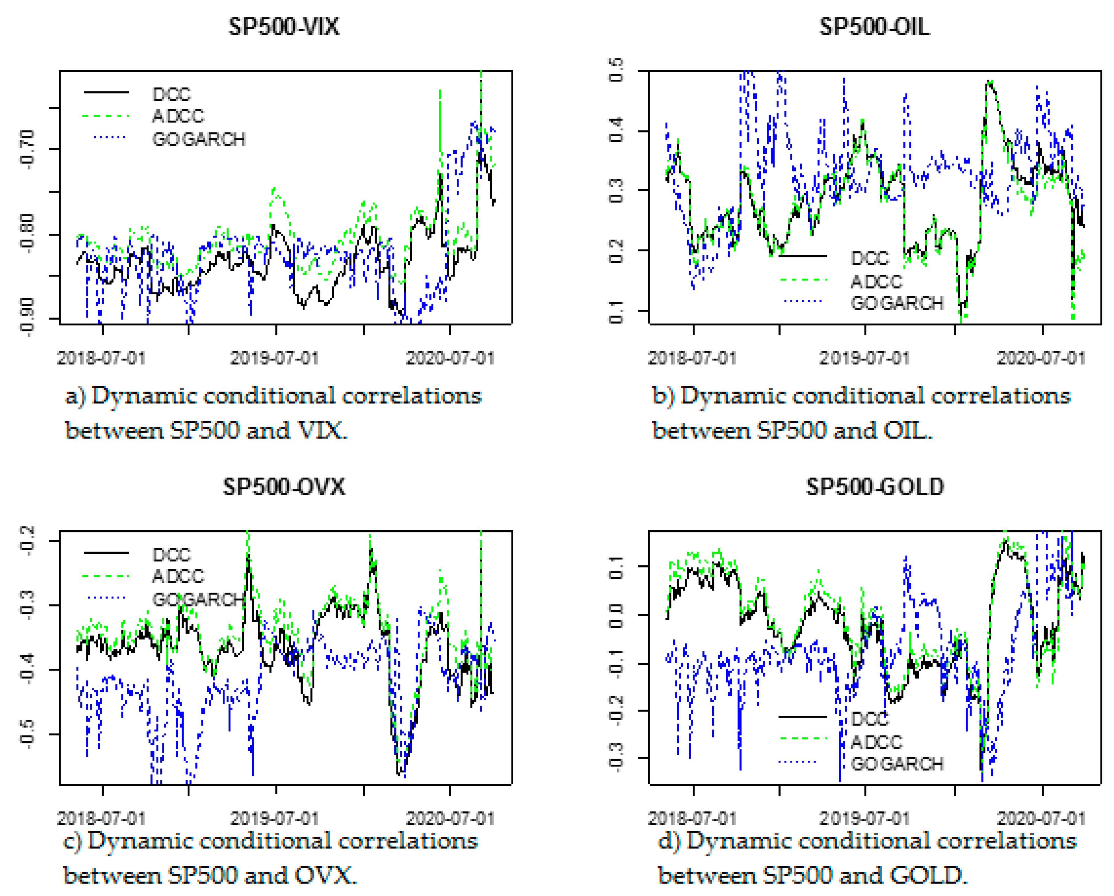
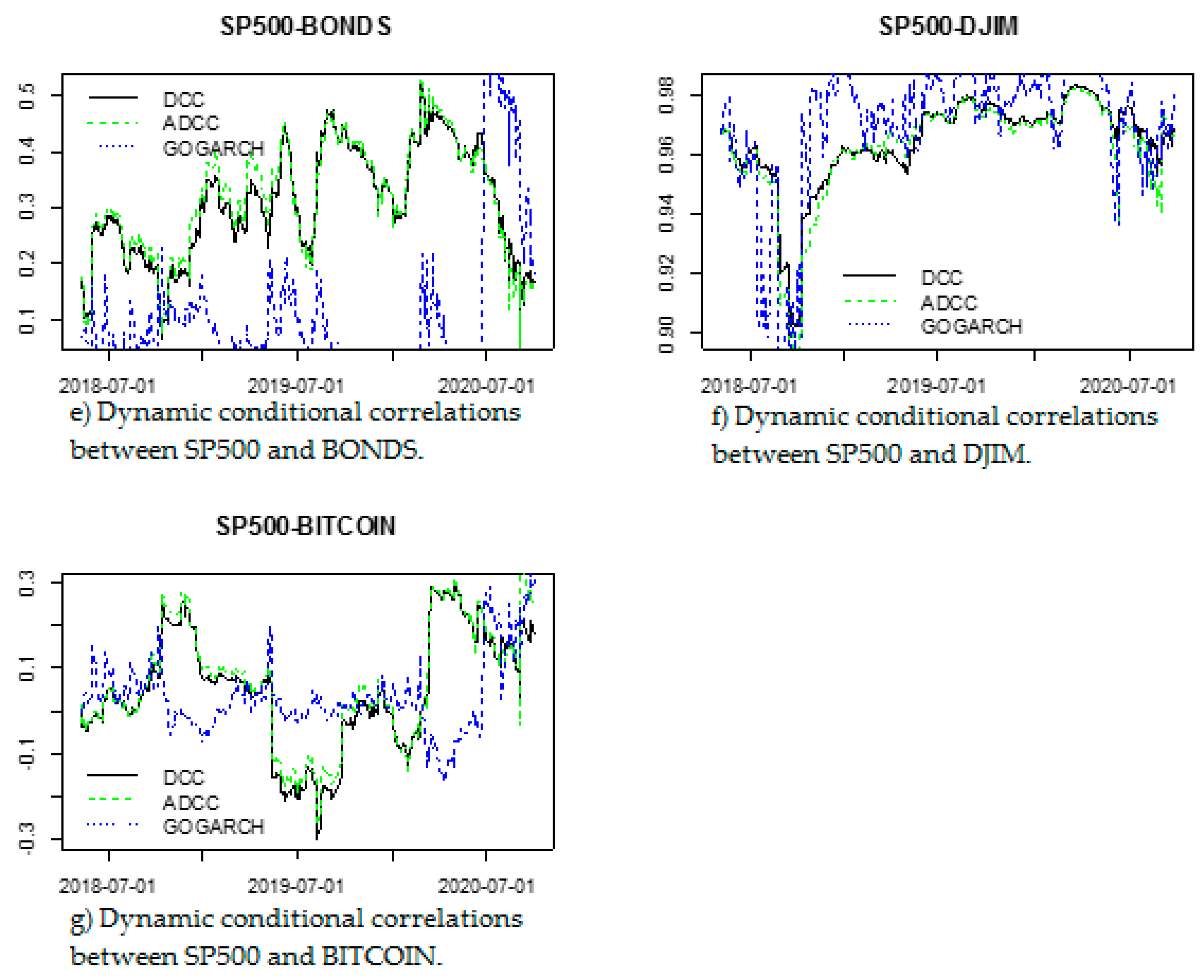
To construct one-step ahead dynamic conditional correlations, we use rolling window analysis. The estimation window is fixed at 2425 observations, and 600 dynamic conditional correlations one-step ahead are produced. GARCH models are refitted every 266 observations. Considering that the linkages between stocks and all variables change over time, we examine the time-varying dynamic conditional correlation of the market pairs. The results are presented in Figure 2a–g.

From the visual inspection of the dynamic correlations graphs, we establish first that the correlations between the S&P500 stock market and all variables are time-varying and highly volatile. Overall, we find that the dynamic conditional correlation between all return pairs fluctuates greatly during our sample period, which indicate that portfolio managers and investors should adjust their portfolio structure frequently. During the most of the sample period, the dynamic conditional correlations among market pairs are positive, indicating the spillover effects. However, in some periods, though short, the conditional correlation is negative for some pairs, indicating that investors may gain more from a portfolio diversification strategy.

Let us examine separately, one by one, the dynamic conditional correlations that obtained from the GARCH models between US stock market and each assets. For SP500/VIX and SP500/OVX pairs, the dynamic conditional correlations are negative for the three GARCH models, suggesting significant diversification benefits. The inverse relationship between the SP500 and VIX (OVX) means that stock markets tend to lose money when volatility or uncertainty increases.

The SP500/OIL pair show contrary findings, the conditional dynamic correlations are decisive values. The dynamic correlations produced from the three models are very high, especially during the fast spread period of COVID-19 in the US at the end of the first quarter of 2020 (March 2020), compared to the dynamic correlations during 2019.

The dynamic conditional correlations between SP500 and GOLD fluctuates between negative and positive values. The negative correlation between gold and equities is not a new phenomenon, as several studies (see Shahzad et al. 2017) showed that the negative relationship indicates that gold is an instrument of hedge and it is a safe-haven asset for stock markets during crisis periods. On the contrary, Basher and Sadorsky (2016) reported for emerging markets a positive relationship between gold and equities because of heavy demand for gold coming from China and India. In the case of the SP500/BONDS pair, the dynamic conditional correlations fluctuates between negative and positive values. The negative correlation SP500/BONDS is probably the result of the so-called “Bernanke put”, which may be attributed to the lower yield on the 10-year Treasury bonds. Considering that the positive correlation between SP500 and BONDS, the correlation may reflect investors’ “on/off” approach to asset allocation (flight to quality) due to the gradual reduction planned by the Federation of its quantitative policy easing triggered a sell-off in the U.S. stock market (S&P500).

On the other hand, for the SP500/DJIM pair, we noted that the positive dynamic conditional correlations are very high compared to the all assets. While the SP500/BTC pair show a weaker dynamic conditional correlations, they fluctuate between negative and positive values during the sample period.

From the dynamic correlation findings, we can conclude that during the recent health and economic-financial crisis, the correlations produced using the GARCH models are positive and have reached the highest level during the spread of the coronavirus period in the United States compared to the pre-COVID-19 period, which indicates that this health crisis supports the risk spillover. Except for SP500/VIX and SP500/OVX, the dynamic conditional correlations are still negative.

In comparison between the GARCH models, we noted that the time-varying conditional correlations estimated from DCC and ADCC models exhibit similar patterns. In contrast, the GO-GARCH model produces different patterns. For each examined pair, the correlations between the dynamic conditional correlations produced from the DCC and ADCC model are highly correlated (

Table 5. Correlation matrix.

	SP500/VIX	SP500/OIL	SP500/OVX	SP500/GOLD	SP500/BONDS	SP500/DJIM	SP500/BTC
DCC/ADCC	0.975	0.990	0.985	0.991	0.993	0.993	0.989
DCC/GO-GARCH	0.105	0.368	0.107	0.106	0.177	0.772	0.425
ADCC/GO-GARCH	0.138	0.364	0.133	0.103	0.173	0.774	0.429

This table is a correlation matrix between each pair of variables considered, depending on the underlying specification.

). For each pair of conditional correlations, the correlations between DCC and GO-GARCH or ADCC and GO-GARCH are less correlated, except for SP500/DJIM, which is consistent with Figure 3. For SP500/DJIM pairs, the conditional correlations produced from the DCC and GO-GARCH, also ADCC and GO-GARCH are highly correlated, but less than the correlations between DCC and ADCC for each pair.

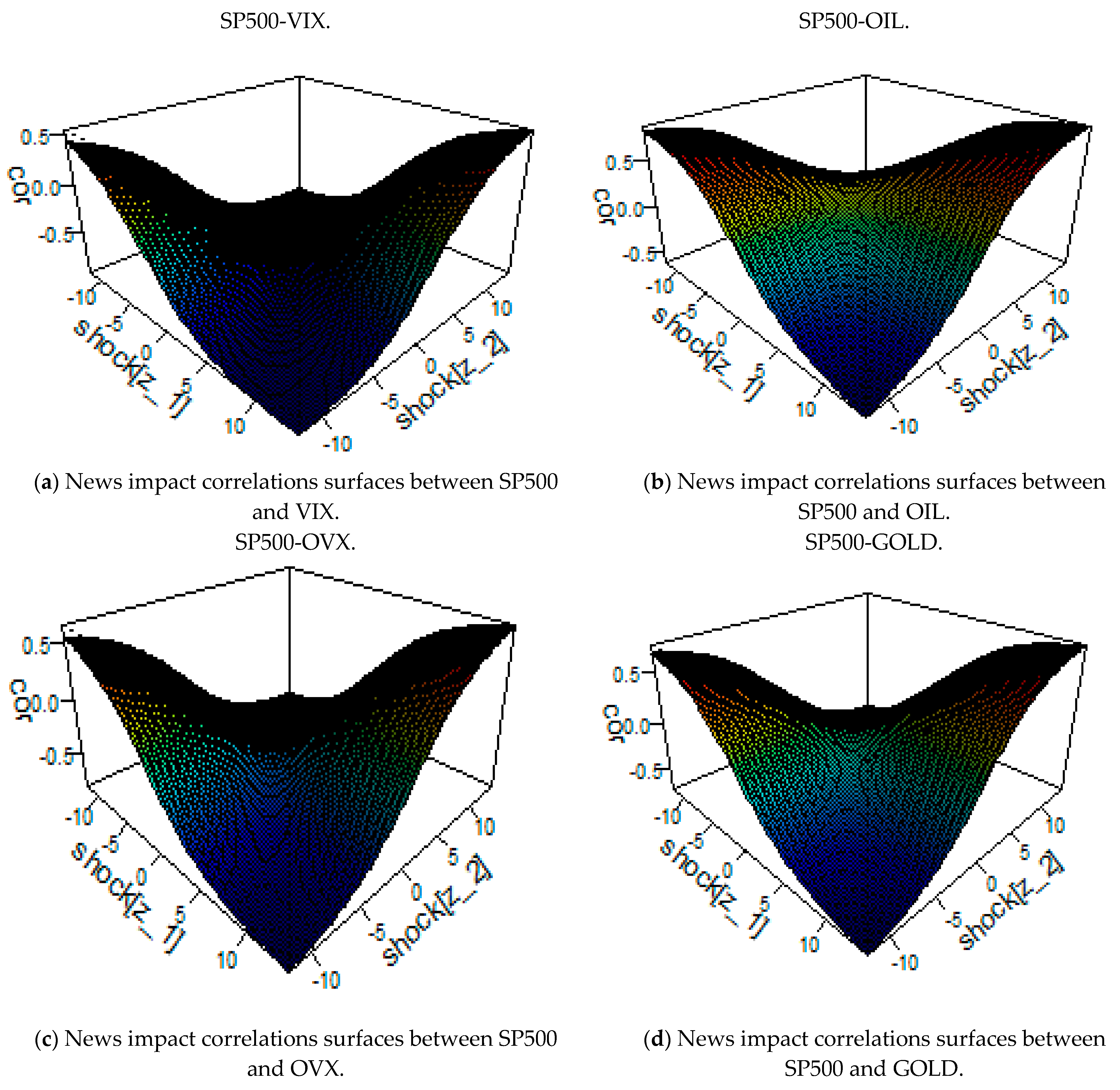
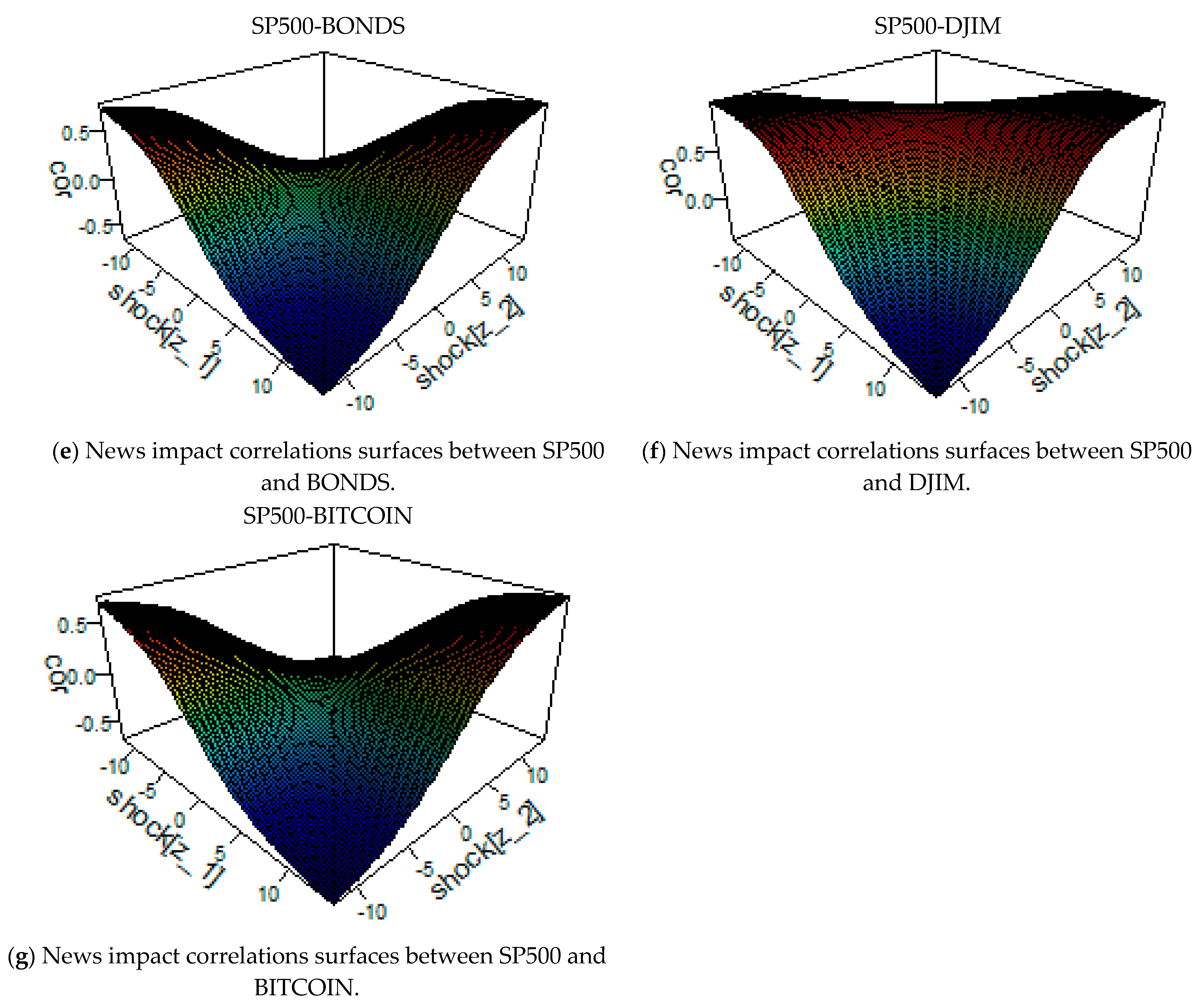
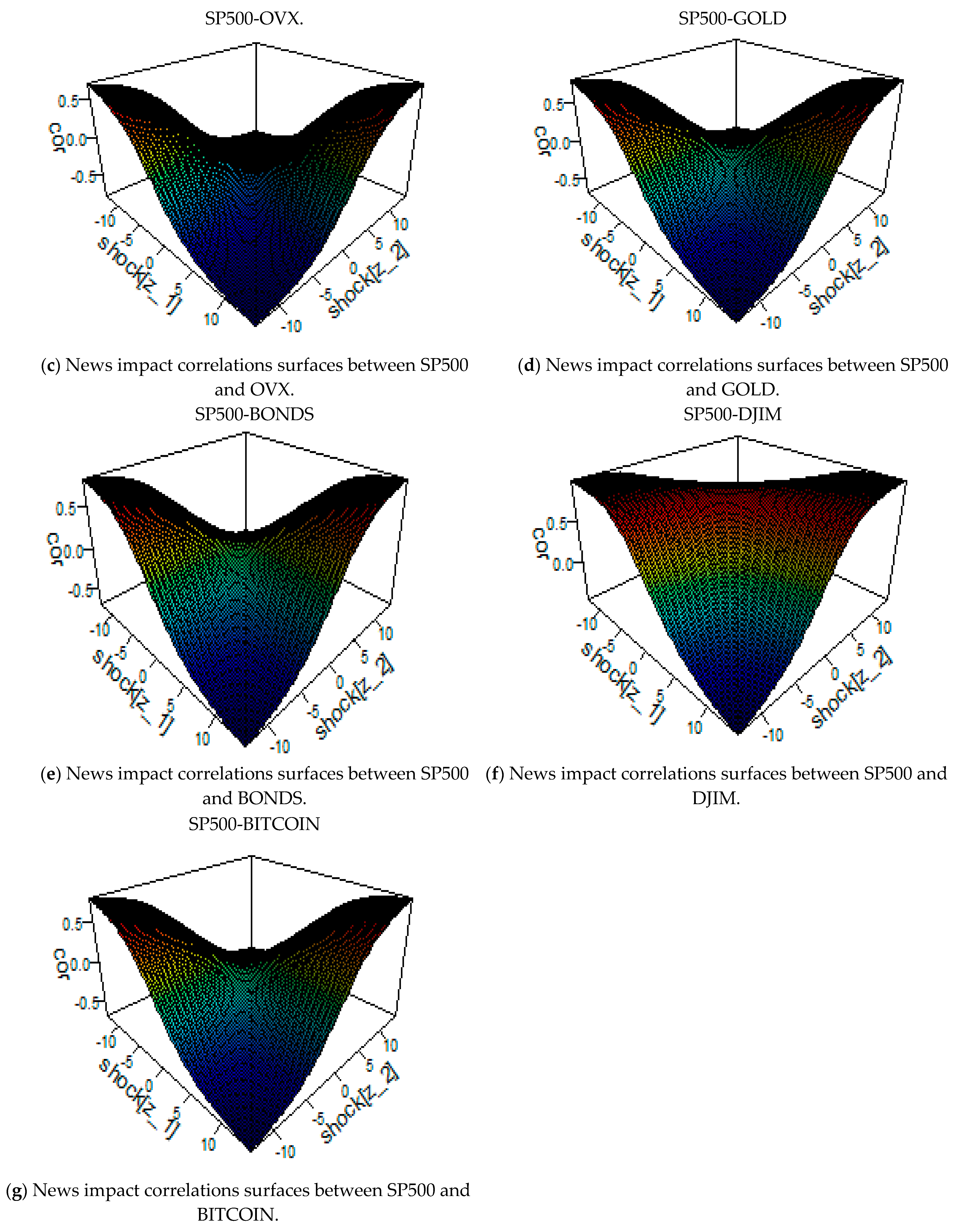
Further to the analysis of conditional correlations, we extended our analysis in this paper and we investigate the news impact correlations surfaces between each pair (Appendix C). We find that the news impact correlations surface produced from DCC and ADCC models show a similar shape, while the GO-GARCH model shows a different shape. The couple pairs shows that the news impact correlations surface produced from the DCC or ADCC models indicate that shocks have asymmetrical effects on the correlation between SP500 and each asset. While, the news impact correlations surfaces produced from the GO-GARCH model show more symmetric impact of shocks in correlation between SP500 and the remains assets. This is expected since the GO-GARCH factors are orthogonal. Moreover, we find that the shapes of new impact correlation surfaces produced from the DCC and ADCC models for each pair are convex, while the shapes produced from the GO-GARCH are concave for SP500/VIX, SP500/OVX, SP500/GOLD, and SP500/DJI, the shapes of the remains pairs are convex.

4.3. Analysis of Optimal Hedge Ratios and Hedging Performance

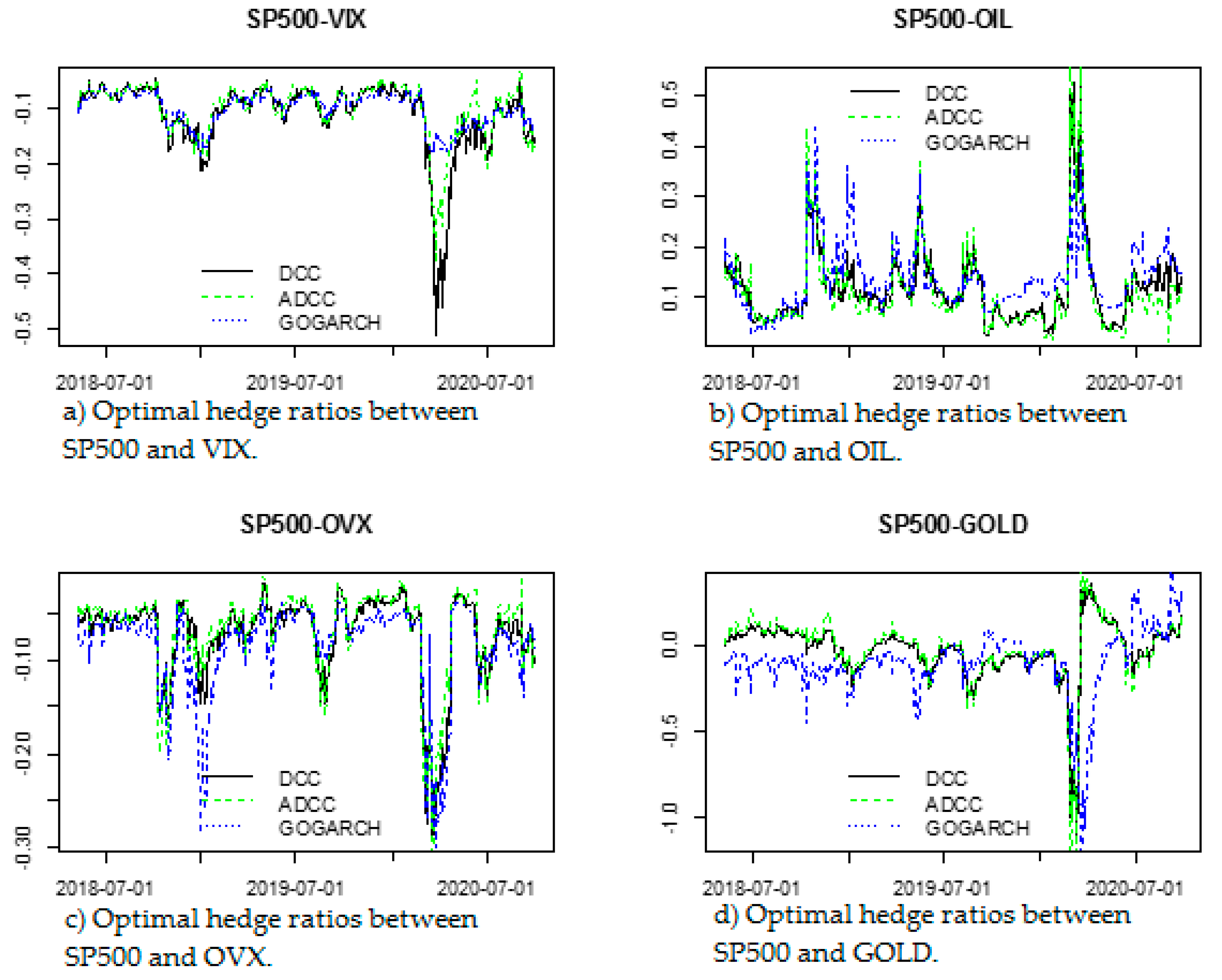
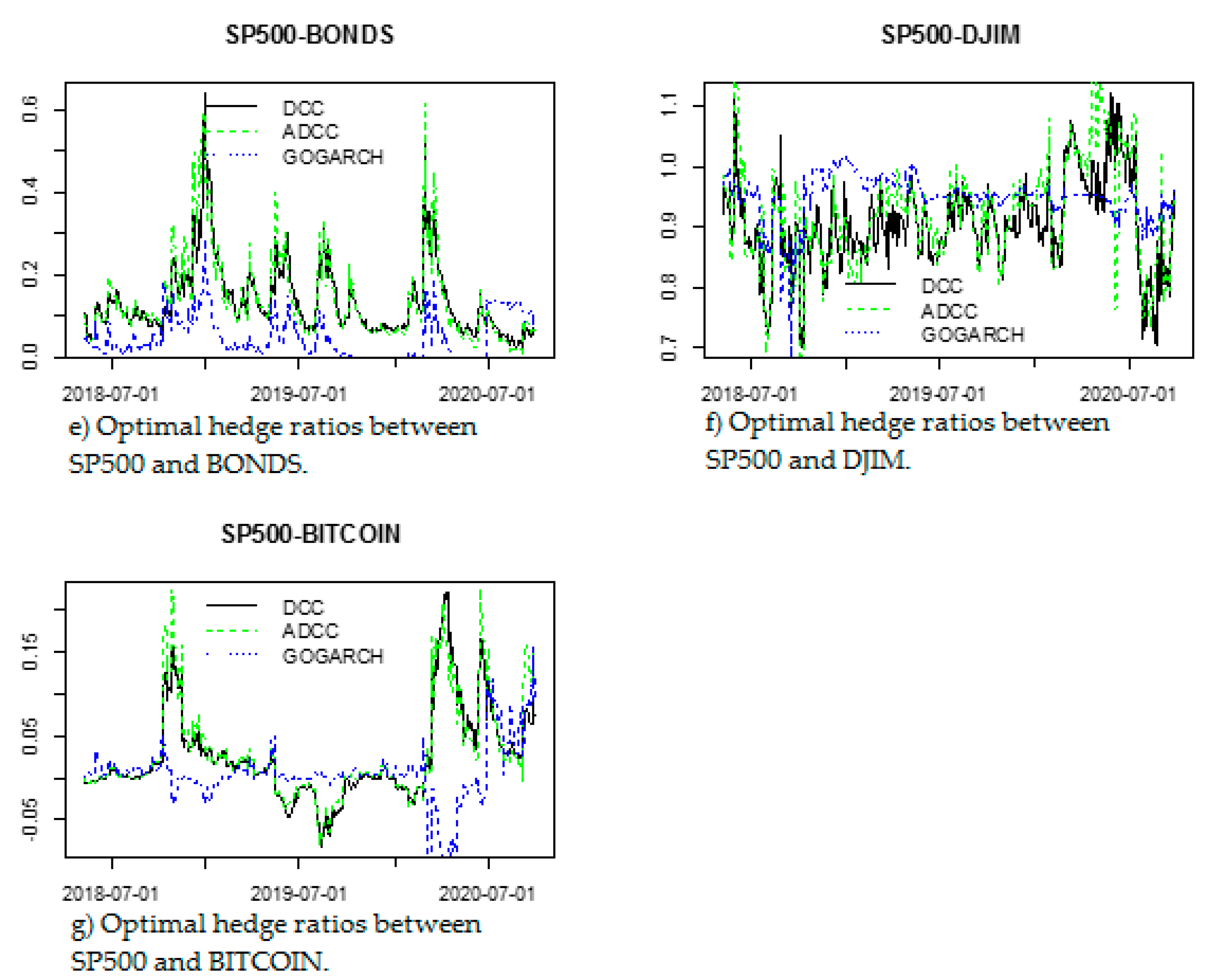
Using the rolling window analysis, we construct the out-of-sample hedge ratios. At period t, a one-period-ahead conditional volatility forecast for a period is established, these forecasts are used to build a one-period-ahead hedge ratio. All forecast hedge ratios are later used for the construction of the hedged portfolio. A rolling window size of 2425 observations is used to construct 600 one-period-ahead hedge ratios. GARCH models are refitted every 266 observations.

4.3.1. Optimal Hedge Ratios Plots

Figure 3a–g shows the optimal hedge ratios plots calculated between SP500 and a position in VIX, OIL, OVX, GOLD, BONDS, DJIM, and BTC.

We can see from the plots that optimal hedge ratios have high variability for most pairs for three models. The optimal hedge ratios SP500/VIX and SP500/OVX pairs are negative. This happens because these pairs are negatively correlated. The optimal hedge ratios between SP500/OIL and SP500/DJIM pairs are positive. While for SP500/GOLD, SP500/BONDS, and SP500/ BTC pairs, the hedge ratios are fluctuating between positive and negative values.

The weaker variability of hedge ratios is more likely observed produced by the GO-GARCH model compared to the DCC and ADCC models. For each pair, we noted that the high levels of optimal hedge ratios during the period of the substantial spread of the coronavirus in the United States. Except for SP500/VIX and SP500/OVX, the optimal hedge ratios are still negative. The same cases like the dynamic correlation, we also noted that the optimal hedge ratios patterns produced by the GO-GARCH model are different from those of DCC and ADCC, which are very similar patterns.

Table 6. Correlation between hedge ratios.

	SP500/VIX	SP500/OIL	SP500/OVX	SP500/GOLD	SP500/BONDS	SP500/DJIM	SP500/BTC
DCC/ADCC	0.964	0.974	0.971	0.983	0.984	0.975	0.988
DCC/GO-GARCH	0.317	0.059	0.090	0.058	−0.253	0.776	0.008
ADCC/GO-GARCH	0.332	0.059	0.106	−0.001	−0.289	0.778	0.048

This table displays the correlation between hedge ratios computed for each pair of variables considered.

shows the correlation between hedge ratios. We find that the hedge ratios produced from the DCC and ADCC model are highly correlated more than the correlations between DCC and GO-GARCH or ADCC and GO-GARCH, which is consistent with Figure 3.

4.3.2. Hedge Ratio Summary Statistics and Hedging Effectiveness

We present in

Table 7. Hedge ratio summary statistics and hedging effectiveness (HE).

		Mean	Min	Max	HE
SP500/VIX	DCC	−0.113	−0.513	−0.045	0.612
	ADCC	−0.101	−0.381	−0.033	0.604
	GO-GARCH	−0.101	−0.190	−0.061	0.597
SP500/OIL	DCC	0.120	0.026	0.534	0.041
	ADCC	0.113	0.014	0.589	0.044
	GO-GARCH	0.140	0.028	0.437	0.063
SP500/OVX	DCC	−0.072	−0.293	−0.016	0.145
	ADCC	−0.066	−0.312	−0.009	0.198
	GO-GARCH	−0.084	−0.301	−0.035	0.052
SP500/GOLD	DCC	−0.031	−1.130	0.362	−0.097
	ADCC	−0.018	−1.372	0.440	−0.116
	GO-GARCH	−0.102	−1.341	0.428	−0.342
SP500/BONDS	DCC	0.024	−0.082	0.222	0.166
	ADCC	0.029	−0.082	0.225	0.122
	GO-GARCH	0.046	−0.040	0.290	0.130
SP500/DJIM	DCC	0.904	0.702	1.120	0.981
	ADCC	0.919	0.650	1.211	0.980
	GO-GARCH	0.947	0.685	1.017	0.979
SP500/BTC	DCC	0.024	−0.082	0.222	0.118
	ADCC	0.029	−0.082	0.225	0.127
	GO-GARCH	0.005	−0.143	0.156	−0.098

Hedge ratios calculated from fixed width rolling analysis which produces 600 one-step forecasts. Models are refit every 266 observations. GARCH models estimated using a multivariate t (MVT) distribution. All specifications include a constant and an ARMA (1,1) term in the mean equation.

the hedge ratio summary statistics and hedging effectiveness between US markets and the potential hedge assets. We can see that the average value of hedge ratios between SP500 and the two implied volatility indexes is negative because these pairs of assets are negatively correlated. The same case for GOLD. On the other hand, the average value of the hedge ratio between SP500 and the remains assets is positive. SP500 and Islamic market have the high average of hedge ratio where it is 90 cents for the DCC model indicating that a $1 long position in SP500 can be hedged for 90 cents in the Islamic market. By comparison, the average value of the SP500/DJIM hedge ratio is 91 cents when computed using the ADCC model and 94 cents when using the GO-GARCH model. Using the GARCH models, we calculate the hedging effectiveness between US stock market and each asset. We find that Islamic assets are the most desirable hedge for the SP500 than VIX, OIL, OVX, BONDS, and BITCOIN. In comparison, we document that the DCC model has a high hedging effectiveness for SP500/VIX, SP500/GOLD, SP500/BONDS, and SP500/DJIM pairs than the GO-GARCH model, which it produces low effective hedge (except SP500/BONDS). The ADCC model has high hedging effectiveness for SP500/OVX and SP500/BTC pairs than the GO-GARCH model, it produces lower hedging performance. For SP500/OIL, the GO-GARCH model produces the most effective hedge while the DCC model produces the least effective. One possible reason for this is that the second and the third factor in the GO-GARCH has higher short-term persistence and lower long-term persistence which is better suited to capture the dynamics in this hedge.

Our results shows that the three models confirm that SP500/DJIM has higher hedging effectiveness than other pairs. VIX provides the second most effective hedge followed by BONDS and BITCOIN in third order. We can conclude that the Islamic market is the better hedge asset when it is combined with the US equity market during the sample period including the short period of the COVID-19 pandemic crisis.

4.4. Results Discussion

The results of time-varying conditional correlations show that the risk spillover during the COVID-19 period has reached the highest level compared to the pre-COVID period. This last one can lead us to an important conclusion where, the pandemic supports the contagion effect, which increase the risk spillover between US stock markets and different financial variables and commodities. We expected this finding because the COVID-19 pandemic works as a systematic risk which caused harmful consequences for financial markets and the economy. A similar observation unveiling the peaking of correlations during the COVID-19 global pandemic has been found in recent literature (Chevallier 2020, 2021; Akhtaruzzaman et al. 2020; Zhang et al. 2020; Zaremba et al. 2020). The U.S. stock market reacted so much more forcefully to COVID-19 than to previous pandemics, such as the Spanish flu (Baker et al. 2020). The high degree of correlations during the COVID-19 crisis supports strong evidence about the contagion effect of the COVID-19 pandemic on the connectedness between each couple pairs during the implementation of containment in the U.S. Since the COVID-19 outbreak, keeping in view the uncertainties concerning the end date of the pandemic and the rise of infection cases and deaths by the COVID-19 pandemic in the world was associated with a reduced value stock markets for short terms and increase the uncertainty and the fear in financial markets. This was expected because the governments in many countries have enforced some confinement policies like social distancing and border shutdowns, travel restrictions, and the general quarantine in countries which constitute the world’s largest economies to mitigate the spread of the virus, thus the health pandemic transformed to become the worst financial recession since the 1929 crisis.

The implied volatility index shows a negative connectedness with the equity market which explores significant diversification benefits (Basher and Sadorsky 2016). However, over the COVID-19 period, a smoothed stability in the dynamic conditional correlation between VIX (OVX) and SP500 during our sample period suggests the absence of additional economic benefits of diversification. As we have said previously, COVID-19 acts as a systematic risk that cannot be diversified and which caused hard financial and economic consequences.

Furthermore, looking to the findings of hedging analysis, they have important implications for investors in the US equity market. From a speculators and portfolio managers’ perspective, we can say that an investor seeking higher yields from S&P500 index exposure while hedging risk in their portfolios should combine it with the Islamic market. This is mainly because the hedging effectiveness is highest for the SP500/DJIM pair. Therefore, a hedging strategy can be implemented by taking a position on both assets. The high optimal hedge ratios relating to the Islamic market may be explained by the fact that Islamic agreements are noted and subject to revisions during the period of detention. This study shows that the DJIM is the best hedge asset either in the tranquil or crisis period. Therefore, the Islamic equities can serve as the best hedge asset for the investments in the U.S. stock index (S&P500) against extreme market conditions. In fact, over the short last period relating to the COVID-19 pandemic outbreak, our results confirm that these stock market indices still provide the best hedging effectiveness compared to the rest of the assets. Notice that taken together, the results above suggest that the higher the correlation between assets, the more suitable they are as a hedging instrument. However, using the opposite position of the highly correlated asset, it is easier to use options or futures contract on the same instrument to diversify the risk. The implied volatility index shows the second best hedging effectiveness. These results are consistent with those of Hood and Malik (2013) and Ahmad et al. (2018). From the previous studies, we noted that there is a huge debate in the literature about the Bitcoin, if is it really a valuable hedging tool and safe-haven asset for equity markets or not. Our paper adds to the most previous studies that limit their scope to testing the hypothesis that Bitcoin is a safe haven without capturing practical implications in terms of hedging effectiveness (Bouri et al. 2017b). We confirm that the virtual currency BTC can be a hedge asset for the US market, where it provides the third best effective hedge. We can explain this by the weak correlation of Bitcoin with traditional assets, making it a very potent diversification tool (Baur et al. 2018; Bouri et al. 2017a, 2017b; Briere et al. 2015; Corbet et al. 2018; Guesmi et al. 2019; Ji et al. 2018) and a valuable hedge for equities (Baur et al. 2018; Bouri et al. 2017a; Shahzad et al. 2020). Finally, we noted that some hedging effectiveness values are negative which indicates hedged portfolios are worse than unhedged portfolios.

5. Conclusions

Quantifying the economic impact of the COVID-19 pandemic is a complex task due to the sharp rise in the uncertainty about the economic and financial outlook. The variety of risks associated with this global spread of the new virus affected the world from various sides. The abrupt rise in uncertainty results in low economic growth and significant financial instability. A sharp increase in economic uncertainty, as measured approximately by the equity market volatility, is mostly observed around the world irrespective of the level of economic development of the economy. For instance, in the Euro area, the United States and Japan GDP fell abruptly. Investors strove to incorporate the latest risks induced by the sanitary crisis.

In comparison, between the pre-COVID-19 and COVID-19 crisis, our study is useful to financial advisors who often seek unconventional assets that can provide protection for stock portfolios against downside risk, especially during stress periods when protection is rewarding. The purpose of our analysis was to model volatility spillovers, investigate the dynamics of conditional correlations, and estimate optimal hedge ratios to identify the assets that provide the highest hedge effectiveness for US stock market returns (S&P500). We focused on energy and precious metal commodities (especially oil and gold) through their hedging capacity. Most studies highlight the hedge of stock market returns, as well as the implied volatility indexes (VIX, OVX), the spot interest rate (Bonds), the Islamic stock (the Dow Jones Islamic), and cryptocurrencies (Bitcoin).

We use daily data and span the period from 3 February 2011, to 29 September 2020. We have a total of 2425 observations. The analysis sample includes specifically the recent COVID-19 crisis period, leading investors to look for the best hedge asset or the best diversification strategy to smooth their exposition to risk.

The main findings of the study present interesting results. Both DCC and ADCC models confirms that the volatility of recent return has a significant influence on the dynamic relationship between the U.S. stock market and all indices. This can be observed for the considerable value of the coefficient of dynamic conditional correlations, indicating that the dynamic co-movement between the equity market and all other variables is persistent.

Through the lens of dynamic conditional correlations, we establish that the time-varying conditional correlations show that the conditional correlation of all return pairs fluctuating greatly during our sample period, which means that investors and portfolio managers should adjust their portfolio structure frequently. In most of the sample period, the dynamic conditional correlation among market pairs is positive and supports the contagion effects. However, in some periods, though short, the conditional correlation is negative for some pairs, indicating that investors may gain more from a portfolio diversification strategy, especially, the two implied volatility indexes VIX and OVX shows significant diversification benefits. During the pandemic, COVID-19 acts as a systematic risk that cannot be diversified, and which caused hard financial and economic consequences.

On the other hand, the second axis of the paper provides a valuable finding. Looking to the results of hedging analysis, we document that the optimal hedge ratios between SP500 and a position in VIX, OIL, OVX, GOLD, BONDS, DJIM, and BTC have higher variability and increase significantly in most cases, implying higher hedging costs, especially during the COVID-19 period. The SP500/DJIM pair have the higher hedge effectiveness over the entire sample, including a short period relating to the recent COVID-19 crisis. The Dow Jones Islamic is the best hedge asset for U.S. equity, either in tranquil or crisis periods, during the pre-COVID-19 and COVID-19 period. VIX gives the second best hedging effectiveness for S&P500. Bonds and Bitcoin provides the third best hedging effectiveness alternatives.

The results of our study are in line with some previous research arguing that during the COVID-19 pandemic, the risk spillover (contagions effect) increases between financial markets (e.g., Yousfi et al. 2021; Akhtaruzzaman et al. 2020; Zhang et al. 2020; Zaremba et al. 2020; Chevallier 2020, 2021). The implied volatility index suggests the diversification benefits, a finding confirmed with the empirical results of Abid et al. (2020a, 2020b); Ahmad et al. (2018). The main takeaway from this paper is that the Islamic market exhibits the most effective hedge for SP500 stock prices followed by VIX, BONDS, and BITCOIN, respectively, under our considered assumptions. This is a new result. The most recent studies on hedging U.S. equities document that commodity markets are the best hedge assets against the risks (Abid et al. 2020b; Junttila et al. 2018; Chkili et al. 2014; Raza et al. 2018; Shahzad et al. 2020). These latter results may have some practical implications for speculators, investors, and portfolio managers; they should be give more attention on the risk management during their portfolio construction to diversify and hedge their risk during the extreme risk period like the COVID-19 crisis. However, they should know that COVID-19 acts as a systematic risk that cannot be diversified.

References

- Abid, Ilyes, Abderrazak Dhaoui, Khaled Guesmi, and Olfa Kaabia. 2020a. Hedging strategy for financial variables and commodities. Economics Bulletin 40: 1368–79. [Google Scholar]
- Abid, Ilyes, Abderrazak Dhaoui, Stéphane Goutte, and Khaled Guesmi. 2020b. Hedging and diversification across commodity assets. Applied Economics 52: 2472–92. [Google Scholar] [CrossRef]
- Ahmad, Wasim, Perry Sadorsky, and Amit Sharma. 2018. Optimal hedge ratios for clean energy equities. Economic Modelling 72: 278–95. [Google Scholar] [CrossRef]
- Akhtaruzzaman, Md, Sabri Boubaker, and Ahmet Sensoy. 2020. Financial contagion during COVID-19 crisis. Finance Research Letters 38: 101604. [Google Scholar] [CrossRef] [PubMed]
- Arouri, Mohamed El Hedi, Amine Lahiani, and Duc Khuong Nguyen. 2015. World gold prices and stock returns in China: Insights for hedging and diversification strategies. Economic Modelling 44: 273–82. [Google Scholar] [CrossRef] [Green Version]
- Ashraf, B. N. 2020. Stock markets’ reaction to Covid–19: Cases or fatalities? Research in International Business and Finance 54: 101249. [Google Scholar] [CrossRef]
- Baker, Scott R., Nicholas Bloom, Steven J. Davis, Kyle Kost, Marco Sammon, and Tasaneeya Viratyosin. 2020. The unprecedented stock market reaction to COVID-19. The Review of Asset Pricing Studies 10: 742–58. [Google Scholar] [CrossRef]
- Basher, Syed Abul, and Perry Sadorsky. 2016. Hedging emerging market stock prices with oil, gold, VIX, and bonds: A comparison between DCC, ADCC, and GO-GARCH. Energy Economics 54: 235–47. [Google Scholar] [CrossRef] [Green Version]
- Baur, Dirk G., and Brain M. Lucey. 2010. Is gold a hedge or a safe haven? An analysis of stocks, bonds, and gold. Financial Review 45: 217–29. [Google Scholar] [CrossRef]
- Baur, Dirk G., KiHoon Hong, and Adrian D. Lee. 2018. Bitcoin: Medium of exchange or speculative assets? Journal of International Financial Markets, Institutions and Money 54: 177–89. [Google Scholar] [CrossRef]
- Boswijk, H. Peter, and Roy Van der Weide. 2006. Wake Me Up before You GO-GARCH (No. 06-079/4). Tinbergen Institute Discussion Paper. Amsterdam and Rotterdam: Tinbergen Institute. [Google Scholar]
- Boswijk, H. Peter, and Roy Van der Weide. 2011. Method of moments estimation of go-garch models. Journal of Econometrics 163: 118–26. [Google Scholar] [CrossRef] [Green Version]
- Bouri, Elie, Naji Jalkh, Peter Molnár, and David Roubaud. 2017a. Bitcoin for energy commodities before and after the December 2013 crash: Diversifier, hedge or safe haven? Applied Economics 49: 5063–73. [Google Scholar] [CrossRef]
- Bouri, Elie, Peter Molnár, Georges Azzi, David Roubaud, and Lars Ivar Hagfors. 2017b. On the hedge and safe haven properties of Bitcoin: Is it really more than a diversifier? Finance Research Letters 20: 192–98. [Google Scholar] [CrossRef]
- Briere, Marie, Kim Oosterlinck, and Ariane Szafarz. 2015. Virtual currency, tangible return: Portfolio diversification with bitcoin. Journal of Asset Management 16: 365–73. [Google Scholar] [CrossRef]
- Broda, Simon A., and Marc S. Paolella. 2009. Chicago: A fast and accurate method for portfolio risk calculation. Journal of Financial Econometrics 7: 412–36. [Google Scholar] [CrossRef]
- Cappiello, Lorenzo, Robert F. Engle, and Kevin Sheppard. 2006. Asymmetric dynamics in the correlations of global equity and bond returns. Journal of Financial Econometrics 4: 537–72. [Google Scholar] [CrossRef]
- Chang, Chia-Lin, Michael McAleer, and Roengchai Tansuchat. 2011. Crude oil hedging strategies using dynamic multivariate GARCH. Energy Economics 33: 912–23. [Google Scholar] [CrossRef] [Green Version]
- Chevallier, Julien. 2020. COVID-19 pandemic and financial contagion. Journal of Risk and Financial Management 13: 309. [Google Scholar] [CrossRef]
- Chevallier, Julien. 2021. COVID-19 Outbreak and CO2 Emissions: Macro-Financial Linkages. Journal of Risk and Financial Management 14: 12. [Google Scholar] [CrossRef]
- Chkili, Walid, Chaker Aloui, and Duc Khuong Nguyen. 2014. Instabilities in the relationships and hedging strategies between crude oil and US stock markets: Do long memory and asymmetry matter? Journal of International Financial Markets, Institutions and Money 33: 354–66. [Google Scholar] [CrossRef]
- Ciner, Cetin, Constantin Gurdgiev, and Brain M. Lucey. 2013. Hedges and safe havens: An examination of stocks, bonds, gold, oil, and exchange rates. International Review of Financial Analysis 29: 202–11. [Google Scholar] [CrossRef]
- Corbet, Shaen, Andrew Meegan, Charles Larkin, Brain Lucey, and Larisa Yarovaya. 2018. Exploring the dynamic relationships between cryptocurrencies and other financial assets. Economics Letters 165: 28–34. [Google Scholar] [CrossRef] [Green Version]
- Corbet, Shaen, Charles Larkin, and Brain Lucey. 2020a. The contagion effects of the COVID–19 pandemic: Evidence from Gold and Cryptocurrencies. Finance Research Letters 35: 101554. [Google Scholar] [CrossRef]
- Corbet, Shaen, Yang Hou, Yang Hu, Brain Lucey, and Les Oxley. 2020b. Aye Corona! The contagion effects of being named Corona during the COVID–19 pandemic. Finance Research Letters 38: 101591. [Google Scholar] [CrossRef]
- Dyhrberg, Anne Haubo. 2016. Bitcoin, gold, and the dollar—A GARCH volatility analysis. Finance Research Letters 16: 85–92. [Google Scholar] [CrossRef] [Green Version]
- El Mehdi, Imen Khanchel, and Asma Mghaieth. 2017. Volatility spillover and hedging strategies between Islamic and conventional stocks in the presence of asymmetry and long memory. Research in International Business and Finance 39: 595–611. [Google Scholar] [CrossRef]
- Engle, Robert. 2002. Dynamic conditional correlation: A simple class of multivariate generalized autoregressive conditional heteroskedasticity models. Journal of Business & Economic Statistics 20: 339–50. [Google Scholar]
- Glosten, Lawrence R., Ravi Jagannathan, and David E. Runkle. 1993. On the relation between the expected value and the volatility of the nominal excess return on stocks. The Journal of Finance 48: 1779–801. [Google Scholar] [CrossRef]
- Goodell, John W. 2020. COVID–19 and finance: Agendas for future research. Finance Research Letters 35: 101512. [Google Scholar] [CrossRef]
- Guesmi, Khaled, Samir Saadi, Ilyes Abid, and Zied Ftiti. 2019. Portfolio diversification with virtual currency: Evidence from bitcoin. International Review of Financial Analysis 63: 431–37. [Google Scholar] [CrossRef]
- Hood, Matthew, and Farooq Malik. 2013. Is gold the best hedge and a safe haven under changing stock market volatility? Review of Financial Economics 22: 47–52. [Google Scholar] [CrossRef]
- Ji, Qiang, Dayong Zhang, and Yuqian Zhao. 2020. Searching for safe-haven assets during the COVID–19 pandemic. International Review of Financial Analysis 71: 101526. [Google Scholar] [CrossRef]
- Ji, Qiang, Elie Bouri, Rangan Gupta, and David Roubaud. 2018. Network causality structures among Bitcoin and other financial assets: A directed acyclic graph approach. The Quarterly Review of Economics and Finance 70: 203–13. [Google Scholar] [CrossRef] [Green Version]
- Junttila, Juha, Juho Pesonen, and Juhani Raatikainen. 2018. Commodity market based hedging against stock market risk in times of financial crisis: The case of crude oil and gold. Journal of International Financial Markets, Institutions and Money 56: 255–80. [Google Scholar] [CrossRef]
- Kliber, Agata, Pawel Marszałek, Ida Musiałkowska, and Katarzyna Świerczyńska. 2019. Bitcoin: Safe haven, hedge, or diversifier? Perception of Bitcoin in the context of a country’s economic situation—A stochastic volatility approach. Physica A: Statistical Mechanics and Its Applications 524: 246–57. [Google Scholar] [CrossRef]
- Kroner, Kenneth F., and Jahangir Sultan. 1993. Time-varying distributions and dynamic hedging with foreign currency futures. Journal of Financial and Quantitative Analysis, 535–51. [Google Scholar] [CrossRef]
- Ku, Yuan-Hung Hsu, Ho-Chyuan Chen, and Kuang-hua Chen. 2007. On the application of the dynamic conditional correlation model in estimating optimal time-varying hedge ratios. Applied Economics Letters 14: 503–9. [Google Scholar] [CrossRef]
- Lucey, Brain M., and Sile Li. 2015. What precious metals act as safe havens, and when? Some U.S. evidence. Applied Economics Letters 22: 35–45. [Google Scholar] [CrossRef]
- Moran, Matthew T., and Srikant Dash. 2007. VIX futures and options: Pricing and using volatility products to manage downside risk and improve efficiency in equity portfolios. The Journal of Trading 2: 96–105. [Google Scholar] [CrossRef]
- Raza, Naveed, Sajid Ali, Syed Jawad Hussain Shahzad, and Syed Ali Raza. 2018. Do commodities effectively hedge real estate risk? A multi-scale asymmetric DCC approach. Resources Policy 57: 10–29. [Google Scholar] [CrossRef]
- Sadorsky, Perry. 2012. Correlations and volatility spillovers between oil prices and the stock prices of clean energy and technology companies. Energy Economics 34: 248–55. [Google Scholar] [CrossRef]
- Sadorsky, Perry. 2014. Modeling volatility and correlations between emerging market stock prices and the prices of copper, oil, and wheat. Energy Economics 43: 72–81. [Google Scholar] [CrossRef]
- Shahzad, Syed Jawad Hussain, Elie Bouri, David Roubaud, and Ladislav Kristoufek. 2020. Safe haven, hedge and diversification for G7 stock markets: Gold versus Bitcoin. Economic Modelling 87: 212–24. [Google Scholar] [CrossRef]
- Shahzad, Syed Jawad Hussain, Naveed Raza, Muhammad Shahbaz, and Azwadi Ali. 2017. Dependence of stock markets with gold and bonds under bullish and bearish market states. Resources Policy 52: 308–19. [Google Scholar] [CrossRef] [Green Version]
- Sharif, Arshian, Chaker Aloui, and Larisa Yarovaya. 2020. COVID–19 pandemic, oil prices, stock market, geopolitical risk, and policy uncertainty nexus in the U.S. economy: Fresh evidence from the wavelet-based approach. International Review of Financial Analysis 70: 101496. [Google Scholar] [CrossRef]
- Silvennoinen, Annastiina, and Susan Thorp. 2013. Financialization, crisis, and commodity correlation dynamics. Journal of International Financial Markets, Institutions, and Money 24: 42–65. [Google Scholar] [CrossRef] [Green Version]
- Szado, Edward. 2009. VIX futures and options: A case study of portfolio diversification during the 2008 financial crisis. Journal of Alternative Investments 12: 68–85. [Google Scholar] [CrossRef]
- Tang, Ke, and Wei Xiong. 2012. Index investment and the financialization of commodities. Financial Analysts Journal 68: 54–74. [Google Scholar] [CrossRef]
- Van der Weide, Roy. 2002. GO-GARCH: A multivariate generalized orthogonal GARCH model. Journal of Applied Econometrics 17: 549–64. [Google Scholar] [CrossRef]
- Vivian, Andrew, and Mark E. Wohar. 2012. Commodity volatility breaks. Journal of International Financial Markets, Institutions, and Money 22: 395–422. [Google Scholar] [CrossRef]
- Wątorek, Marcin, Stanisław Drożdż, Jarosław Kwapień, Ludovico Minati, Paweł Oświęcimka, and Marek Stanuszek. 2020. Multiscale characteristics of the emerging global cryptocurrency market. Physics Reports 901: 1–82. [Google Scholar]
- Yousfi, Mohamed, Younes Ben Zaied, Nidhaleddine Ben Cheikh, Béchir Ben Lahouel, and Houssam Bouzgarrou. 2021. Effects of the COVID-19 pandemic on the US stock market and uncertainty: A comparative assessment between the first and second waves. Technological Forecasting and Social Change 167: 120710. [Google Scholar] [CrossRef]
- Zaremba, Adam, Renatas Kizys, David Y. Aharon, and Ender Demir. 2020. Infected Markets: Novel Coronavirus, Government Interventions, and Stock Return Volatility around the Globe. Finance Research Letters 35: 101597. [Google Scholar] [CrossRef] [PubMed]
- Zhang, Dayong, Min Hu, and Qiang Ji. 2020. Financial markets under the global pandemic of Covid–19. Finance Research Letters 36: 101528. [Google Scholar] [CrossRef] [PubMed]
- Zhang, Kun, and Laiwan Chan. 2009. Efficient factor garch models and factor-dcc models. Quantitative Finance 9: 71–91. [Google Scholar] [CrossRef]
Figure 1.
Times series plots.
Figure 2.
Rolling one-step-ahead conditional correlations. (a) Present the dynamic conditional correlations between Scheme 500. and VIX; (b) Present the dynamic conditional correlations between SP500 and OIL; (c) Present the dynamic conditional correlations between SP500 and OVX; (d) Present the dynamic conditional correlations between SP500 and GOLD; (e) Present the dynamic conditional correlations between SP500 and BONDS; (f) Present the dynamic conditional correlations between SP500 and DJIM; (g) Present the dynamic conditional correlations between SP500 and BITCOIN.
Figure 3.
Rolling one-step-ahead optimal hedge ratios. (a) Present the hedge ratios between SP500 and VIX; (b) Present the hedge ratios between SP500 and OIL; (c) Present the hedge ratios between SP500 and OVX; (d) Present the hedge ratios between SP500 and GOLD; (e) Present the hedge ratios between SP500 and BONDS; (f) Present the hedge ratios between SP500 and DJIM; (g) Present the hedge ratios between SP500 and BITCOIN.