
Do Financial Professionals Process Information Better as a Group Than Non-Professionals?
1
Department of Accounting, Smeal College of Business, The Pennsylvania State University, State College, PA 16801, USA
2
School of Accountancy, Coles College of Business, Kennesaw State University, Kennesaw, GA 30144, USA
*
Author to whom correspondence should be addressed.
†
Deceased.
J. Risk Financial Manag. 2021, 14(5), 230; https://0-doi-org.brum.beds.ac.uk/10.3390/jrfm14050230
Submission received: 25 February 2021
/
Revised: 1 May 2021
/
Accepted: 12 May 2021
/
Published: 20 May 2021
(This article belongs to the Section Applied Economics and Finance)
Abstract
:In this study, we study information processing by financial professionals benchmarked with non-professionals and how correlation among individual forecasts explains the group level forecast performance. In an experiment in which participants make price forecasts based on common financial information, we find that individual professionals are no better than individual non-professionals in forecasting, but professionals’ mean forecasts are superior. Our analysis suggests that financial professionals’ individual errors are less correlated as they process information from more diverse perspectives. This leads to superior mean forecasts because the uncorrelated individual errors cancel each other out in the aggregate. In contrast, non-professionals are similar in using salient information such as earnings or cash flow. As a result, their individual errors are highly correlated. Instead of cancelling each other out, the individual errors are enlarged in the aggregated mean forecasts. We are the first to show the difference in the comparisons of professionals and non-professionals at the group level versus at the individual level. Our paper contributes to the literature by documenting the evidence of diversity in information processing by financial professionals.
1. Introduction
Researchers have called for more evidence concerning the nature of financial professionals’ expertise (Ramnath et al. 2008). Such professionals are widely employed by both large and small institutions. Often, these supposedly more sophisticated professionals cover the same firms’ stock. The nature of the expertise provided by these groups of professionals, however, remains unclear, because the effects of averaging forecasts by a group of financial professionals remain unclear. If financial professionals within the groups share common information and process information in a similar way, then their forecasts errors will be highly correlated and tend to add up instead of cancelling out in the average forecasts.
A major difference of our study from the prior research is the focus on group performance instead of individual performance. Prior research in accounting and psychology mostly focuses on the individual difference between professionals and non-professionals. The existing findings suggest that professionals’ information processing differs from non-professionals in a variety of ways, including information search, strategy selection, weights attached to data when arriving at conclusions, and final conclusions (see reviews in Libby et al. 2002; Maines 1995; Trotman et al. 2011; Anderson 1988). In contrast, we focus on comparing the group performance difference between professionals and non-professionals. The implication of our finding is that constructing a group—or composite—forecast from individual forecasts is more useful when sourcing these forecasts from professional investors than from nonprofessional investors.
Most importantly, we show that the comparison at the individual level does not necessarily translate into the same comparison at the group level. The important factor that determines group level performance is the correlation among the individuals’ judgement, not just the quality of individual judgement. A group with individuals who have low forecast accuracy but think differently can have superior group performance than a group with individuals who have high forecast accuracy but think in the same way. In group forecasts, uncorrelated errors cancel out so that more diverse knowledge collectively leads to superior group performance.
The prior literature indicates that experts’ judgments are highly correlated (e.g., Broomell and Budescu 2009). Existing archival data using analysts’ earnings forecasts also suggest that professional analysts are highly correlated in their information processing. The level of professional agreement about upcoming earnings has been viewed as typically high and increasing over time (e.g., Noreen et al. 1985, p. 133). Potential explanations for this seemingly high and increasing agreement included: (i) professionals employ similar procedures to process information, (ii) they use a common information set, (iii) they share information with each other information about their forecasts, and (iv) they have incentives to conform to the average forecast (Noreen et al. 1985, p. 133). All of these explanations are consistent with professionals being primarily conduits of common financial information. Additionally, while prior research shows evidence that incentives to conform to the average forecast are limited (e.g., Barron et al. 2002), there is little direct evidence as yet with regard to the first explanation (i.e., that professionals process information similarly), because information processing is unobservable in archival data. Using an experiment, we fill in this gap by directly examining the information processing among financial professionals benchmarked with those from non-professionals.
Our comparison of professionals to non-professionals is motivated in part by intuition that suggests that, in contrast to professionals, non-professionals’ information processing may be more heterogeneous. If so, then compared to financial professionals, the forecast errors of the group of non-professionals may be less correlated, thus causing the mean forecast of non-professionals to contain a richer set of information than the mean financial professionals’ forecast. Thus, professionals as a group may be inferior to non-professionals as a group even if individual professionals tend to be superior to individual non-professionals. Shiller (2005) points out this possibility that “Institutional investors as a group are not necessarily smarter than individual investors as a group” (Shiller 2005, p. 119). Additionally, it is possible that professionals’ forecasts add little to the overall accuracy of forecasts aggregated across all investors’ forecasts. If the correlation in forecast errors between the professional group and non-professional group is high, then the price forecasts of professionals may add little value to the average overall forecast. To make a contribution to the aggregate belief, professional forecasts must convey unique information that is not highly correlated with that of non-professionals.
To the extent that the market reflects and aggregates the consensus of non-professional and professional investors, the consensus of non-professionals provides us with a benchmark to evaluate the incremental contribution of professional investors. While the earnings forecasts of professionals are available for archival studies, the forecasts of non-professionals are not. Thus, we collect experimental data by asking professional and non-professionals to make price forecasts based on common financial information. The controlled experiment offers two main advantages. First, we can hold constant the information available to both professionals and non-professionals to focus on their processing of information, while controlling for other possible explanations such as differences in information access or herding incentives. Second, we can ask participants to tell us how they use information in forecasting, which directly sheds light on the commonality of information processing itself.
We send out a questionnaire with a common set of financial information to participants. Our data includes responses from 69 professional investors and 121 non-professional investors. Employment experience is the critical distinction between the two groups. In particular, professionals’ job functions involve stock recommendations (e.g., financial analysts, brokers, investment advisor, fund manager, portfolio manager). We find that individual professionals’ stock price forecasts are not significantly more accurate than those of non-professionals. Yet, the professionals’ forecasts as a group are more accurate than the non-professionals as a group. To show why this is true, we use a measure of the correlation in forecast errors advanced by Barron et al. (1998, hereafter BKLS). We find that this measure of correlation is significantly lower for professionals than for non-professionals. As a result, professionals in aggregate (and not individual professionals) outperform non-professionals. Furthermore, we find that the forecast errors of the non-professionals are highly correlated with the forecast errors of professionals, and the average price forecast of non-professionals contains little or nothing that would be new to professionals. In fact, non-professionals are “strictly dumber” than professionals, in that averaging in the price forecasts of non-professionals makes the overall price forecast less accurate.
The intuition behind our result can be illustrated using an example. Suppose the true value is 5. Non-professionals might both make a forecast of 7. Therefore, they are wrong by 2. Professionals might make forecasts of 3 and 7, because they process information from different perspectives. On average, non-professionals are not worse than professionals as they both make average individual forecast errors of 2. However, when we average the professional forecasts, we get the true value of 5, whereas the non-professionals remain at 7. In this way, the average of professional forecasts is more accurate than the average of non-professionals.
In addition to reporting price forecasts, participants also reported the weight they put on various pieces of information. We find that the weights put on different types of financial information vary more for the professionals than the non-professionals. Apparently, the private expertise of professionals makes them less susceptible as a group than non-professionals to fixating on any particular type of information. This evidence complements evidence in archival studies. Using published earnings forecasts, Barron et al. (2002) conclude that the correlation in analysts’ forecast errors typically decreases after earnings announcements. The stark evidence in our experiment shows that the relative advantage of professionals is driven primarily by the diverseness in information processing. This highlights the value of groups of financial professionals in security markets.
Our paper contributes to the recent literature that investigates the behavioral of financial professionals. Existing studies examine the individual attributes such as information processing (Anderson 1988; Andersson 2004; Hodge and Pronk 2006), behavioral biases or anomalies (Cohn et al. 2015; Haigh and List 2005; Kiymaz et al. 2016; Roth and Voskort 2014). In practice, however, multiple financial professionals often cover the same firm. Thus, the collective behavior of the group is important to understand the value of financial professionals in a market setting. We are the first to consider the group-level performance of professionals benchmarked with non-professionals, and contrast it with the comparison of professionals and non-professionals’ performance at the individual level. Most importantly, we find that financial professionals’ forecast errors are less correlated with each other, which explains why their group-level performance is superior. Contrary to the conventional beliefs that financial professionals are more similar to each other due to their common financial training, we find that the diversity of information processing by a group of financial professionals is greater than a group of non-professionals.
2. Conceptual Underpinnings and Hypotheses
2.1. Conceptual Underpinnings
Research in accounting and psychology has examined how and why professionals’ judgment and decision making differs from those of novices (Libby et al. 2002; Maines 1995; Trotman et al. 2011; Anderson 1988). They mostly focus on the individual performance. Libby and Luft (1993) provide a theoretical framework to analyze individual decision performance. Specifically, decision performance is a function of ability, experience, and knowledge. Experience affects performance through knowledge. In other words, they suggest that much of experienced decision makers’ advantage lies in their larger knowledge stores and, more importantly, the manner in which they organize their knowledge.
In our setting, for example, professionals such as financial analysts may have knowledge of sophisticated models. Professionals tend to have more training in the finance area. Their education and training give them knowledge about sophisticated financial models that can be useful to analyze financial data. This is likely to lead to higher individual forecast precision if the models are useful for forecasting. However, it is unclear how the knowledge about sophisticated models affects forecast diversity among the professional group. If their training involves similar models, and they tend to use the same models (for example, the Capital Asset Pricing Model based on market beta), then their forecasts are likely to be similar to each other. On the other hand, non-professionals have background in different areas and are likely to think from their own area-specific perspectives. Our study mainly focuses on the comparison between the degree of diversity in forecasting by professionals and non-professionals. How difference in individual forecasting improves the composite forecasts at the group level is the unique perspective adopted by our study.
Prior research has pointed out that the individual-level performance can be very different from the group-level performance. In particular, there are significant benefits of constructing composite group judgments from individual judgments. Bonner (2008, p. 235) states that “composite group JDM quality frequently exceeds individual JDM quality… these outcomes occur because composites of individual judgments and decisions cancel random errors and also can cancel bias if individuals have JDM biases that go in opposite directions.” Our paper considers how this error cancellation mechanism explains the performance difference between the professionals and non-professionals. This differentiates our paper from the existing literature that compares professionals and non-professionals, which mainly focus on individual-level performance.
2.2. Hypotheses
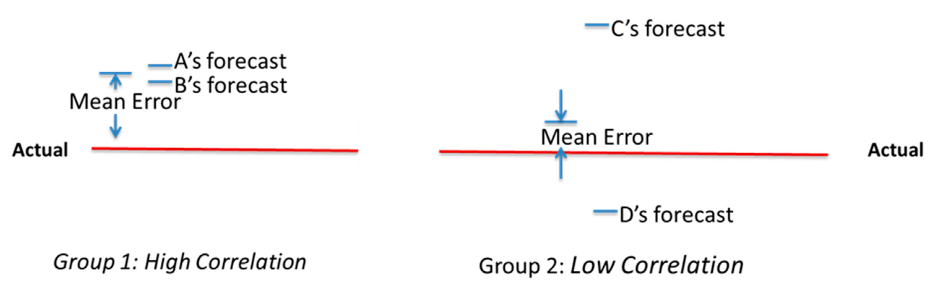
The impact of correlation in forecast errors on the accuracy of group forecasts can be seen from the following example. Suppose there are two forecasters, A and B, in group 1, and two forecasters, C and D, in group 2. Figure 1 shows a hypothetical case that demonstrates the important role of commonality (or correlation) within a group in affecting the accuracy of the group forecasts.
As shown in Figure 1, individual forecast accuracy for both A and B is higher than C and D. However, A and B’s forecast errors are correlated, while C and D’s forecast errors are not. Taking the average of group 1 forecasts adds up the errors in A and B, while taking the average of group 2’s forecasts cancels out the errors in C and D. Thus, the mean forecast error of group 2 is smaller than the mean forecast error of group 1, despite the fact that individual forecasters in group 2 are less accurate than group 1.
In our controlled experiment, subjects are provided with a common set of information about the same set of firms. Their forecasts are likely to have positively correlated errors for the following reasons. First, subjects face the common variation in fundamentals when evaluating the same asset. Second, subjects receive the same financial information about the asset. The common information source contains the same noise that can lead to positively correlated errors. In addition, subjects may make common mistakes in processing information. The similarity in processing information can also cause positive correlation in forecasts errors. However, subjects may process the same information in different ways. This diversity in information processing can reduce the correlation among subjects’ forecasts. If subjects process information in a more diverse manner, the correlation in forecasts errors is lower. In aggregate, idiosyncratic errors are diversifiable and can cancel each other out. Therefore, consensus forecasts are more accurate if the group of subjects share fewer common errors.
Whether financial professionals or non-professionals have less correlation in information processing is an empirical question. The direct empirical evidence on the degree of diversity of information processing by professionals and non-professionals is lacking. Our paper fills in this gap. We apply the BKLS model in Barron et al. (1998) to estimate the proportion of information that is common relative to information that is individual-specific using observable attributes of individual and consensus forecasts. When the information processing is more diverse, the BKLS measure of proportion of common information is smaller.
Benchmarking nonprofessionals with professionals allows us to evaluate the relative degree of diversity of information processing by professional investors. Both professionals and nonprofessionals face the same variation in fundamentals and noise in the information source. The difference in information processing is the only possibility that can cause the BKLS measure of proportion of common information to differ between the professional and nonprofessional group. If the BKLS measure of information commonality is lower for the professionals than the nonprofessionals, we can infer that the information processing by professionals is more diverse than nonprofessionals.
We define as the average squared error in individual non-professionals’ price forecast errors, and as the correlation (or commonality) of these errors across non-professionals. Likewise, we define as the average squared error in individual professionals’ price forecast errors, and as the correlation (or commonality) of these errors across professionals. and are the number of forecasts, respectively. From the BKLS model, we get the following relation when the average squared error in the mean forecast (SE) is equal across the two groups:
By inspection, it can be seen that average squared error in the mean forecast decreases as the number of forecasts increases. However, the number of forecasts does not have to be very large for this effect to be negligible, and for our purposes, both analytically and experimentally, we assume the groups of professionals and non-professionals to be large so that and are negligible. Thus, we focus on the following expression:
Of course, the non-professionals’ forecasts would likely always tend to “add value” to the degree that their average error was uncorrelated with the average error of professionals. To the degree that this was true, the two groups of errors may tend to cancel each other out. We assume that this effect is likely to be minimal, however, because when all investors have access to the same information (as they do in our experiment), it is likely that the information that is commonly inferred will also be the information that is the most easily inferred. Thus, non-professionals are likely to be able as a group to infer all or most of what is commonly inferred by professionals. As reported later, our empirical evidence confirms that the common (or average) forecast error of non-professionals is very highly correlated with that of professionals.
Thus, a necessary condition for professional forecasts having incremental information content beyond that of non-professionals is . We call this the condition in which professionals are strictly “smarter” as a group than the group of non-professionals. Both the superiority as an individual and the diversity among individuals (correlation) affect the superiority of the group. At the individual level, it is possible that professionals are superior, inferior to, or the same as non-professionals. It is also possible that the correlation among professionals is the same as, higher, or lower than non-professionals. The joint effect of individual superiority and correlation determines the aggregate level superiority.
The comparisons at the individual level are not always consistent with the comparisons at the aggregate level. For example, consider the case where individual professionals do tend to have smaller forecast errors that non-professionals, or . The non-professionals as a group may still be “smarter”, or , if they tend to interpret/process information differently from each other, or . This seems quite plausible and even intuitive. Therefore, there is no ex ante reason for predicting that professionals as a group are strictly smarter than non-professionals. Thus, our main hypothesis is stated in the null form as follows:
Hypothesis 1 (H1).
The aggregate forecast of professionals is no more accurate than the aggregate forecast of non-professionals, or .
We then examine the following two related hypotheses to explore the underlying reason for our findings with regard to the first hypothesis:
Hypothesis 2 (H2).
Professionals’ individual forecasts are of the same accuracy as those of non-professionals, or .
Hypothesis 3 (H3).
The degree of commonality of information in forecasts is the same for professionals as it is for non-professionals, or .
3. Experimental Design and Procedure
Investor sophistication is our main independent variable. Financial professionals are identified as those who have earned their living in the financial services community (with part of their responsibility including stock recommendations). The non-professionals are those who never had employment in the financial sector, but have made some stock investing decisions, no matter how little. Employment experience is the critical distinction between the two groups. Financial expertise is thus defined in terms of employment experience. Specifically, professionals include financial analysts, brokers, bankers, investment advisors, fund managers, portfolio managers, Certified Financial Professionals, fixed income specialists, financial planners, retirement planning specialists, traders, brokerage managers, financial consultants, and Chief Financial Officers.
As different accounting disclosure may trigger different information processing strategies, we varied the accounting disclosure regime to see if our results depended on the accounting disclosure regime. Specifically, we studied three disclosure regimes: earnings only, cash flow only, and both earnings and cash flow. Details about this manipulation are elaborated below when we describe our experimental procedure.
Our study employs a 2 (sophistication) × 3 (disclosure regimes) between-subject design. We used a questionnaire administered online to financial professionals and non-professionals. Both groups were asked to forecast share price changes for firms in the chemical and drug industries in 2008. There was a significant market decline in Year Three, which the subjects were informed about (see Appendix A). The set of instructions provided to each participant contained general economic conditions, stock market data, and outlooks for the chemical and drug industries that were available in the second half of 2008. The participants were not provided the identity of the year, except that it was ‘Year Three.’ The market data were intended to place all participants on the “same page” regarding economic conditions so as to allow differences in forecasts to be more firm-specific. The instructions also provided median financial ratios for the two industries. The ratios were compiled as of the end of Year One (2006), and at the end of Year Two (2007). All information provided to the participants came from the following sources: the Conference Board, the Standard and Poor’s (S&P) Stock Reporter, Wilshire Associates, and Yahoo Financial. In short, all data were compiled from publicly available on-line sources.
Members of both groups of participants were randomly assigned to one of three treatments: earnings treatment, cash flow treatment, and earnings/cash flow treatment. Participants assigned to each of the three treatments received the following common information for each of the 64 observations (32 chemical firms and 32 drug firms): average number of common shares outstanding, Beta, share prices as of the end of Year One and Year Two, and the following balance sheet items on a per share basis as of the end of Year One: cash, current assets, total assets, current liabilities, and long-term debt. Participants assigned to either the earnings treatment or the earnings/cash flow treatment received earnings per share as of the end of Year One and Year Two; participants assigned to either the cash flow treatment or the earnings/cash flow treatment received cash flow per share as of the end of Year One and Year Two.
Each participant was asked to forecast the one-year percentage change in price from Year Two to Year Three for each of the 64 observations. Although there were 64 observations, there were 60 unique firms, as two firms from each industry were repeated. The median ratios in the instructions were those for the variables provided to each respective treatment.
The professional investors were volunteers from various financial institutions; they were a convenience sample recruited by personal contact, referrals, and connections made through LinkedIn. The unsophisticated investors were recruited in a similar manner; many were contacted through their membership in the American Association of Individual Investors. Potential participants received a one-page description of the demands of the study and the potential contributions of the study to the financial services and retail investing communities. Once individuals agreed to volunteer for the study, they were sent three email attachments: a consent statement, a set of instructions, and an Excel spreadsheet. All responses were to be made on the spreadsheet and returned as an email attachment.
In addition to the economic and industry information, the instructions provided guidance to help participants to complete the spreadsheet, such as how to display observations one at a time on computer screens, the format of their responses, and the cells in which to respond. The instructions contained a glossary defining all terms used in the experiment. After participants became familiar with the instructions, they were directed to the Excel spreadsheet. They were additionally encouraged to refer back to the instructions at any time.
The Excel spreadsheet consisted of financial profiles for the 64 observations. By pressing the down arrow keys, subjects could go on to their next observations to make their forecasts. The instructions and spreadsheet clearly indicated that forecasts were to be entered in column C. The profiles consisted of the per share ratios for each observation depending upon the treatment classification. The industry but not the name of each firm was identified. Participants received different orderings of observations. Some participants received a random ordering of drug firms first; others received the chemical firms first, followed by the drug firms. The ordering within each industry group differed. The chemical and drug firms had SIC codes of 281, 282, and 283. The S&P Stock Reporter was also instrumental in selecting firms in that each covered firm was accompanied by a list of related firms. All firms were U.S. companies with a calendar year reporting period. The necessary data for 2006 to 2007 were publicly available for all selected firms.
The Excel spreadsheet also had a debriefing questionnaire following the 64 profiles. The debriefing questionnaire asked biographical questions related to general education, occupation, gender, income, and age. Additionally requested was information related to financial experience such as financial education, belief in efficient markets, risk tolerance, investing experience, and familiarity with the terms used in the study. In addition, questions were asked that were specific to the study, such as familiarity with the chemical and drug industries, level of confidence in one’s forecasts, time to complete the study, level of interest in the study, and the data that most impacted their forecasts. There was one open-ended question in which participants were requested to describe any heuristics and/or “rules of thumb” that assisted them in making their forecasts. On average, participants spent 87 min on the experimental task in total.
4. Experimental Results
This section reports our experimental results. First, we test our hypotheses regarding the comparison between professional and non-professionals using their forecasts. Second, we analyze information processing by examining reported weights on various pieces of financial information.
4.1. Descriptive Data
Our data include responses from 69 professional investors and 121 non-professional investors in three disclosure regimes. Table 1 shows the number of observations for each disclosure regime for the professional and non-professional investors.
Our post-experiment questionnaires provide information about differences in the backgrounds of the professionals and non-professionals. Responses suggest that professionals have more investment experience than non-professionals. We asked participants to indicate how often they have used accounting information in making decisions with respect to investments in common stocks, with level 1 “Never”, level 2 “Once or twice”, level 3 “Not too often, but more than once or twice”, level 4 “Somewhat frequently”, 5 “Frequently” and 6 “Very frequently”. The average response of the professionals is 4.6, and that of the non-professionals is 3.9. The difference is statistically significant (p = 0.0007). In addition, we ask participants to rate their familiarity with the Efficient Market Hypothesis, with 1 indicating yes and 2 indicating no. The average response for the professionals is 1.07 and non-professional is 1.38. This difference is also significantly different (p = 0.0001). Thus, professionals have more investment experience and financial knowledge than non-professionals.
4.2. Hypotheses Tests
Our hypotheses assume that the number of professional and non-professional investors is large enough for each group to be considered the same across groups (see the earlier discussion in Section 2 of the BKLS model), but our number of observations for non-professional investors is about twice that professional investors for all treatments. The number of people in a group is a critical factor in determining the accuracy of group forecasts. The more people are included, the more accurate the group forecasts are if the individual brings new information that others do not have. Thus, to make a fair comparison of group forecasts, we need to make the number of people included in the group forecasts equal. To make the number of people in each group equal while fully using all observations, we adopt the bootstrap method. For example, for the non-professional group with 40 observations, we randomly pick 22 out of the 40 observations. This process is repeated 200 times. Each time, each individual among the 40 observations has equal chances of getting picked. So, we fully use all observations. In our analysis, we bootstrap both the professional and non-professional samples and select the size of the bootstrapped sample to be 22 for both professional and non-professionals for all three treatments. Our bootstrapping procedure samples from the original observations with replacement for 200 replications. We report the mean levels of each test variable in the following tests based on nonparametric tests with bootstrapped samples.
To test H1, we calculate the squared error of the mean forecasts for the professional and non-professional groups in each treatment in our bootstrapped sample. Table 2 reports the averages of the bootstrapped sample.
We conduct a paired nonparametric test of difference for the squared error of mean forecasts using the 64 firm observations for each bootstrapped sample of 22 forecasts. Table 2 reports the average p-value using the Wilcoxon rank test. In all treatments, the average squared error of mean forecasts is significantly smaller for the professional group than the non-professional group. Thus, the null of H1 can be rejected.
Next, we examine H2 by comparing the quality of individual forecasts for the professional and non-professional groups. We calculate the squared error of individual forecasts and then take the average for each group. Table 3 reports the average squared error of individual forecasts for our bootstrapped sample. The average squared error of individual forecasts is not significantly different between the professional and non-professional groups. Thus, the null of H2 cannot be rejected. At the individual level, the professionals do not appear to be much smarter than the non-professionals.
Lastly, we examine H3 by comparing the ρ estimated using the BKLS model for the professional and non-professional groups. Following BKLS, we calculate ρ for each firm using the following equation, where SE is the squared error in the mean forecast, D is the dispersion in forecasts and N is the number of forecasts.1
Using the observed forecasts and actual percentage price changes, we calculate the ex post squared error in mean forecasts, SE.
where A is the actual percentage price change, is the forecasted percentage price change by analyst i, and is the average of the forecasted percentage price change by all analysts for a firm within a treatment cell.
For each of our bootstrapped samples, we calculate the BKLS measures and then conduct a Wilcoxon ranked paired test of the difference between the professional and non-professional groups using the 64 firm observations. Table 4 reports the averages over the 200 bootstrapped samples.
For all treatments, the average estimated ρ for the professional group is significantly lower than that for the non-professional group. This indicates that the professionals’ information processing is more heterogeneous than that of the non-professional group. Thus, the null of H3 can be rejected.
To further explore why professionals as a group have more accurate forecasts than non-professionals, we examine the sign of forecast errors. As shown in Figure 1, group forecasts are more accurate if the sign of errors are more balanced on the positive and negative side. Table 5 reports the average frequency of positive and negative forecast errors by treatments for the two groups.
For all treatments, there are more postive errors than negative errors. This suggests that forecasts tend to be more optimistic. The professionals are less optimistic than non-professionals. The frequency of positive errors are signficantly smaller than non-professionals for all three treatments. All differences between professionals and nonprofessionals are significantly different from each other, with p-value less than 0.001 based on the paired t-test. The errors are more balanced on the positive and negative side for professionals than non-professionals. Consistently with the intuition shown in Figure 1, having more balanced errors leads to more accurate group forecasts.
Furthermore, including the forecasts of the non-professionals in the mean forecast yields worse forecast quality compared to when only the forecasts of professionals are included. The average squared error of mean forecasts which include only the professionals compared with the averaged squared error of mean forecasts which include both the professionals and non-professionals. Paired tests of differences using the Wilcoxon rank test are significant for all treatments.
4.3. Information Weightings
In our post-experiment questionnaires, participants are asked to provide the reported weights they put on each of eleven pieces of information, which include Beta, price, earnings, cash flow, dividends, cash, current asset, total asset, current liability, long term debt, and number of shares. Both professionals and non-professionals put the majority of weight on four pieces of information: Beta, price, earnings and cash flow. Only these four pieces of information receive more than a 10% weight (the max weight is higher than 50%). The rest of the information receives a weight of less than 10%. This suggests that participants paid most attention to the accounting information such as earnings and cash flow, and market-based information such as Beta and price.
Table 6 reports the average weights and the standard deviation of the weights for these four pieces of information for the three disclosure regimes as well as tests of the differences between the professional and non-professional groups.
There is no significant difference in the average weights, but in many cases the standard deviation of the weights for professionals is significantly greater than that of non-professionals. For example, Panel A shows that the weight on earnings for professionals is 23.23, which is similar to that of non-professionals (22.20). However, the standard deviation of the weight on earnings for professionals is much greater than for non-professionals. The standard deviation of the weight on earnings for professionals is 19.62. The weights on earnings mostly vary by +/− one standard deviation, that is, between 3.61 and 42.85. The standard deviation of the weight on earnings for professionals is 12.10. The weights on earnings mostly vary between 10.1 and 34.3. As seen from the two ranges above, there is a greater difference in the weights on earnings among professionals than non-professionals. The standard deviation of the weights for the non-professionals is never significantly greater than that of the professionals. This indicates that the processing of information by the professionals is more diverse compared to the non-professionals.
Table 6 Panel B reports the reported weights on cash flow, price and Beta in the Cash Flow treatment. The standard deviation of the weights for the professionals is significantly greater than that of the non-professionals for two pieces of information: cash flow and price. The standard deviation of the weights on cash flow is 20.32 for the professionals, which is significantly higher than the corresponding standard deviation of 13.30 for the non-professionals (p = 0.02). The standard deviation of the weights on price is 23.14 for the professionals, which is significantly higher than the corresponding standard deviation of 13.32 for the non-professionals (p = 0.003). There are more variations among professionals in the use of cash flow and price information.
Table 6 Panel C reports the reported weights on earnings, cash flow, price and Beta in the Earnings/Cash Flow treatment. The standard deviation of the weights on Beta is 29.99 for the professionals, which is significantly higher than the corresponding standard deviation of 18.75 for the non-professionals (p = 0.01). There are more variations among professionals for the use of beta.
4.4. Robustness Check
The firms in our samples are not independent because they are drawn from the same period and two industries. To address the issue of dependence, we conduct supplementary analysis of our main tests. We use repeated measure ANOVA, employing a mixed model assuming compound symmetry (see Littell et al. 2006), and our main results are robust. In addition, we adopt the demean approach to account for the lack of dependence among firms. Specifically, we take out the industry average forecasted return from each individual forecasted return. At the same time, we take out the actual average industry return from each individual forecasted return. Forecast errors are calculated by benchmarking the adjusted forecasts with the adjusted actual. Our main results are also robust to this approach.
We can rule out the possibility that a few other factors may explain our results on the difference between professionals and non-professionals. In our post-experiment questionnaires, we ask participants to report their level of interest in the study, with level 1 indicating “Uninteresting”, level 2 “Somewhat uninteresting”, level 3 “Somewhat interesting”, and level 4 “Very interesting”. The average interest level for the professionals is 2.75 and for non-professionals is 2.78. There is no significant difference between the two (p = 0.82). Second, we have a measure of time that participants spent on completing the survey. On average, professionals spent 78 min and non-professionals spent 91 min. The difference between the two is not significant (p = 0.14). Thus, the interest in the task and effort in completing the forecasting tasks is not likely to explain our results.
We also ask participants to rate the level of confidence in their forecasts, with level 1 “Not very confident”, level 2 “Confident” and level 3 “Very confident”. The average confidence for professionals is 1.47 and the average confidence for non-professionals is 1.3. The confidence level of the professionals is significantly higher than the confidence level of non-professionals (p = 0.018).
5. Discussion and Conclusions
We conduct a controlled experiment to better understand how financial professionals as a group process public information relative to non-professionals as a group. Providing both groups with the same financial data, we ask professionals and non-professionals to make price forecasts and report their use of information and forecasting strategy. Our results suggest that the professional investors as individuals are not superior to the non-professional investors in making forecasts, but are superior as a group. Our analysis shows that the information processing by professional investors is more heterogeneous, so that forecast errors are less correlated and cancel each other out more than in the non-professional group.
Our theoretical analysis shows that forecast accuracy at the individual level does not always translate into higher forecast accuracy at the group level. In particular, high individual accuracy but low diversity can lead to lower accuracy at the aggregate level. In contrast, low individual accuracy combined with high diversity could lead to higher accuracy at the aggregate level. We demonstrate the impact of diversity in information processing on the accuracy of forecasts at the individual versus aggregate level. The unpredictable nature of a market crash results in a high degree of uncertainty, so that both professionals and non-professionals face a complex forecasting task. In our setting, both professional and non-professional groups adopt heuristic-based valuation models, but professionals are more highly diversified in the models they use compared to non-professionals. We caution readers to be careful in generalizing our results to other settings. In a setting with less uncertainty, it is possible that professionals have better forecasting ability as individuals. Yet, if their forecast errors are highly correlated, it is possible that professionals as a group have lower forecast accuracy than non-professionals as a group. We leave it for future research to explore such other possibilities.
We contribute to the literature investigating the behavior of financial professionals. Recent studies in behavioral finance explore whether experimental findings with students are also present for financial professionals. On the one hand, financial professionals are found to be less prone to behavioral biases such as anchoring (Kaustia et al. 2008) and the false consensus effect (Roth and Voskort 2014). On the other hand, financial professionals are found to exhibit stronger behavioral effects such as a higher degree of myopic loss aversion (Haigh and List 2005), and more risk taking in competitive situations involving rankings (Kirchler et al. 2018). The major difference of our paper from the prior literature is the focus on the group rather than individual attributes. While individuals may suffer biases and make mistakes, their group performance may still be superior if their individual errors are rather random and less correlated. Our study provides evidence that financial professionals have superior group performance because their individual errors are less correlated.
Our study has two major limitations. First, there is no monetary incentive in our study, which may not induce enough effort from the experimental subjects. Since our results focus on the difference between the professional group and nonprofessional group, this lack of incentive is the same for both groups, and therefore it does not necessarily distort our main results or negate the importance of our findings, but the level of results for each group could be different if monetary incentives are provided. Another potential concern is that we cannot rule out the possibility that other individuals did the task since our study is conducted online. Second, there is a large stock price decrease for the set of firms in our study. How professionals’ information processing diversity varies with the economic condition is an interesting question to pursue in future studies.
Our analysis of information processing suggests that more homogenous information processing is one potential explanation for the high correlation among non-professional investors’ forecasts. Using small trades data, Barber et al. (2009) show that trading decisions of non-professional investors are highly correlated and conjecture that this systematic behavior could be driven by behavioral biases such as disposition effects. In archival data, both biases in information processing and behavioral biases in trading decisions are simultaneously at work. Our study, which isolates these factors, suggests that information processing among non-professional investors is relatively homogenous, which may partly explain their findings. Future studies may explore the relationship between biases in information processing and trading.
Author Contributions
Conceptualization, O.E.B. and C.R.E.; data Collection, C.R.E.; data analysis, H.Q.; writing, O.E.B., C.R.E. and H.Q. All authors have read and agreed to the published version of the manuscript.
Funding
This research received no external funding.
Institutional Review Board Statement
The study was conducted according to the guidelines of the Declaration of Helsinki, and approved by the Institutional Review Board of Pennsylvania State University (Protocol code #33414 and date of approval 19 January 2011).
Informed Consent Statement
Informed consent was obtained from all subjects involved in the study.
Data Availability Statement
Data are available upon request.
Acknowledgments
We appreciate the valuable comments from Lucy Ackert, Saurabh Bansal, Steve Huddart, Terrance Odean, and seminar participants at Penn State Accounting seminar and Experimental Finance conference at University of Mannheim 2016.
Conflicts of Interest
The authors declare no conflict of interest.
Appendix A. Instructions
After reading these instructions you will be directed to an Excel spread sheet with financial profiles of actual unidentified firms from the drug and chemical industries. Please save the spread sheet to your desk top or other convenient location before responding to this instrument. You will be asked to provide share price forecasts for these firms, after which you will be asked some background questions. Once you have completed all items, please return the saved and completed Excel spread sheet as an email attachment. Use the email address contained in the email from which you received these instructions.
Before clicking on the Excel spread sheet it is important that you thoroughly read the instructions contained in the remainder of this Word file. Throughout this exercise you will be given information for YEARS ONE and TWO and be asked to make percentage price change forecasts for the one year period from the end of YEAR TWO to the end of YEAR THREE for each of the chemical and drug firms profiled in the spread sheet. Your forecasts and other responses are strictly confidential. This information will be available only to the researchers. Please do not discuss your responses with others. In making your forecasts use only the information contained in the attachments. These instructions are in 3 parts, [A], [B], and [C].
Part [A] provides a brief summary of the general economic conditions for the drug and chemical industries as reported in the financial press around the middle of YEAR THREE. You will also be given median financial ratios for the 32 firms selected from the drug industry and the 32 firms selected from the chemical industry. For each industry, 16 firms will have values for these ratios greater than the medians, and 16 will have values less than the medians. Firm specific values of these ratios will be in the form of financial profiles in the Excel spread sheet. Your observation of these profiles in conjunction with the other information provided in this exercise should form the basis of your one-year percentage price change forecast for each firm. Part [B] has instructions for entering your forecasts on the spread sheet.
Part [C] is a glossary defining the informational items that you will encounter in part [A] of these instructions. Most of these items are included in the financial profiles of the chemical and drug firms. If you are familiar with all of the information provided in Part [A], you may skip Part [C] and go directly to the Excel spread sheet. When working through the Excel spread sheet it is very important that you follow the instructions in Part [B]. At anytime you may refer to any part of the instructions in this Word document. You may use Columns E through L of the spread sheet to make calculations. Do not alter any of the data given in the cells of the spread sheet. If you choose to make calculations in Columns E through L, please include them in the saved spread sheet that you will return as an email attachment.
PART [A]: ECONOMIC CONDITIONS AND MEDIAN RATIOS
The information in this section is abstracted from The Conference Board, the Standard and Poor’s (S&P) Stock Reporter, and Wilshire Associates and pertains to the middle of YEAR THREE.
Industrial production fell steeply during this period, while employment continued to decline. Real GDP growth slowed to a 1.8 percent average annual rate in the first half of YEAR THREE, down from an annual rate of 2.3 percent in the second half of YEAR TWO. Taken together, the behavior of the composite indexes suggests that the economy is unlikely to improve in the near term.
The Wilshire 5000 Total Market Index (full-cap) is a performance measure of the U.S. stock market. This index increased by approximately 4 percent from the end of YEAR ONE to the end of YEAR TWO. However, this index declined by approximately 39 percent from the end of YEAR TWO to the end of YEAR THREE.
Housing and automobile market slowdowns will continue to hinder demand for chemicals into YEAR FOUR. The annual production by the chemical industry, as measured by the Federal Reserve’s production index for chemicals and related products, is expected to continue to rise sluggishly in YEAR THREE. Chemical industry output in YEAR TWO was unchanged from YEAR ONE. The producer Price Index for chemicals and related products in August of YEAR THREE was at a near record high, up 23% from a year earlier. In short, input costs are expected to be expensive, volatile, and driven by swings in energy prices.
Although drug firms had fairly strong sales and earnings for the third quarter of YEAR THREE, subsequent performance is expected to be weaker based on less favorable foreign exchange, poor new product flow and the soft economy. Additionally, drug firms will face tougher environments on the regulatory and political fronts. Key concerns include R&D productivity, and clinical trial risks. Leading drug firms have been affected by negative clinical outcomes on existing and pipeline products. Despite near-term uncertainties over pricing and patent expirations, long-term prospects should be enhanced by demographic growth in the elderly.
Median Ratios for the 32 Drug and 32 Chemical Firms:

The median Beta and average number of shares outstanding across the two years for the 32 Chemical Firms are 1.22 and 71.2 million, respectively. These figures for the 32 Drug Firms are 0.90 and 93.0 million, respectively. Of the 64 firms that you will observe, over 50 had decreases in their share prices from the end of YEAR TWO to the end of YEAR THREE. The median price change was −40 percent. No firm had an increase as large as 40 percent, and no firm had a price change as low as −90 percent.
The financial profiles that you will observe may not necessarily contain all of the above informational items. However, each item is covered in the glossary and addressed in the debriefing questionnaire that contains the background questions at the end of the Excel spread sheet.
PART [B]: SPECIFIC INSTRUCTIONS FOR COMPLETING THE EXCEL SPREAD SHEET
After clicking on the link to access the Excel spread sheet, save it to your desk top or other convenient location. Next, open the Excel spread sheet and you will see a financial profile of a firm from the chemical or the drug industry. After observing this information make sure your cursor is on cell [C23] where you will enter your first percentage price change forecast. Your forecasts will always be entered in column ‘C,’ and in the empty cell to the left of the cell with the word PERCENT. (The format of your forecasts is covered in the next sub-section.) Next, hit the ‘Page Down’ key on your keyboard to take you to the next screen.
The excel spread sheet was prepared on a Dell desk top computer. The view setting is zoom custom 150%. This setting allows the user of a similar computer to view 23 rows and 12 columns, or one profile per screen. This setting also allows one to arrive at the cell in which to enter the next forecast by just hitting the ‘page down’ key. The spread sheet may not be viewable in this manner on certain other computers such as laptops. In such cases it may be necessary to scroll down a few rows to locate the cell to enter the next forecast. Alternatively, you can adjust the custom zoom setting to show 23 rows per screen. For example, 110% may be the appropriate setting for certain laptops.
The firms are clustered by industry. You will make a total of 64 forecasts. Please make sure that none are skipped. The last forecast is made in cell [C1472]. After your last forecast is entered, please follow the instructions for answering the background questions in the debriefing questionnaire portion of the spread sheet. After these questions are answered, please return the saved and completed Excel spread as an email attachment. Additionally, save a copy of your completed spread sheet for about two weeks.
Forecast Format. Please enter your forecasts in the empty cell to the left of the cell with the word PERCENT. All forecasts must be entered as whole numbers. For example, if you forecast the one year percentage price change for a given firm to be twelve percent, your entry should be 12. DO NOT enter 12%, DO NOT enter 0.12. Additionally, do not make entries such as 12.6, enter only whole numbers (i.e., round 12.6 to 13 and enter 13). If you think the price will decline by twelve percent, enter −12; DO NOT use any of the following formats: −12%, −0.12, (−12), −(12)%, (0.12), (12%), etc. Again please use only whole numbers, no fractions, words, decimals, etc. In Sheet 2 of the spread sheet is a sample profile for a fictitious firm to show how your forecasts must be entered.
The next section is Part [C], the glossary. Please refer to it as needed. If it is not necessary for you to use the glossary, please click on the Excel spread sheet that you saved and start making your forecasts. You may return to the glossary or any other part of the instructions in this Word document at anytime during this exercise.
PART [C]: GLOSSARY
Firm No. This is a nondescript code number to enable the researchers to identify the firm.
Beta. This statistic indicates the volatility of a stock’s price. A Beta greater than 1 indicates higher price volatility than that of the stock market in general; lower than 1 indicates relative price stability. A negative Beta indicates price movement in a direction opposite of the market.
Average No. of shares. The number of shares of common stock held by investors (i.e., shares outstanding) at the end of YEAR ONE plus this number at the end of YEAR TWO, divided by two.
The following items are computed on a per share basis. For example, earnings per share are net income divided by the average number of shares.
Price. The last quoted price of a share of common stock as of the end of the year.
Earnings. This performance measure is income for the year divided by the average number of shares of common stock outstanding (i.e., earnings per share).
Cash Flow. This measure is net income minus preferred dividends and plus non-cash charges (e.g., depreciation) divided by the average number of shares of common stock outstanding (i.e., cash-flow per share). Cash flow is similar to the difference between cash received and cash spent from operating a firm’s business.
Dividends. This figure represents the amount of cash a firm has distributed to common shareholders during the year on a per share basis.
The following items are dollar amounts taken from the year-end balance sheets and are also presented on a per share basis; i.e., the amounts reported by the firm on the balance sheet are divided by the average number of common shares outstanding.
Cash. The year-end amounts of currency and other items that are acceptable for deposit at face value; serves as a medium of exchange and provides a basis of measurement for accounting.
Current Assets. These amounts are cash and resources that are reasonably expected to be converted into cash during the normal operating cycle of a business or within one year, whichever period is longer. In addition to cash, common examples of current assets include receivables (amounts owed to a firm by customers), inventories (materials and merchandise that are intended to be sold to customers), and prepaid items (e.g., advanced payment of insurance premiums).
Total Assets. The total resources of a firm measure by the amounts paid by a firm for these resources, examples include current assets, real estate, machines, furniture, vehicles, patents, investments in other firms, etc. Total assets are presented on a per share basis, to obtain a measurement of the size of a firm in millions of dollars, multiple the total assets figure by the average number of common shares outstanding.
Current Liabilities. These are debt obligations that are reasonably expected to be paid using current assets or by creating other current liabilities within one year or one operating cycle, examples include operating liabilities such as accounts payable (e.g., amounts owed to suppliers) and accrued liabilities (e.g., the amount of interest on debt that has accumulated but not paid).
Long Term Debt. These amounts are obligations that are not expected to be paid in cash or other current assets within one year or the normal operating cycle. Examples include the non-current portion of bonds payable and mortgages. In short, these are debts that must be paid in the future.
| 1 | We thank an anonymous reviewer for suggesting this analysis. |
References
- Anderson, Matthew J. 1988. A comparative analysis of information search and evaluation behavior of professional and non-professional financial analysts. Accounting, Organizations and Society 13: 431–46. [Google Scholar] [CrossRef]
- Andersson, Patric. 2004. Does experience matter in lending? A process-tracing study on experienced loan officers’ and novices’ decision behavior. Journal of Economic Psychology 25: 471–92. [Google Scholar] [CrossRef]
- Barber, Brad M., Terrance Odean, and Ning Zhu. 2009. Systematic noise. Journal of Financial Markets 12: 547–69. [Google Scholar] [CrossRef]
- Barron, Orie E., Oliver Kim, Steve C. Lim, and Douglas E. Stevens. 1998. Using Analysts’ Forecasts to Measure Properties of Analysts’ Information Environment. The Accounting Review 73: 421–33. [Google Scholar]
- Barron, Orie, Donald Byard, and Oliver Kim. 2002. Changes in Analysts’ Information around Earnings Announcements. The Accounting Review 77: 821–46. [Google Scholar] [CrossRef]
- Bonner, Sarah E. 2008. Judgment and Decision Making in Accounting. Upper Saddle River: Pearson. [Google Scholar]
- Broomell, Stephen B., and David V. Budescu. 2009. Why are experts correlated? Decomposing correlations between judges. Psychometrika 74: 531–53. [Google Scholar] [CrossRef]
- Cohn, Alain, Jan Engelmann, Ernst Fehr, and Michel André Maréchal. 2015. Evidence for countercyclical risk aversion: An experiment with financial professionals. American Economic Review 105: 860–85. [Google Scholar] [CrossRef] [Green Version]
- Haigh, Michael S., and John A. List. 2005. Do professional traders exhibit myopic loss aversion? An experimental analysis. The Journal of Finance 60: 523–34. [Google Scholar] [CrossRef]
- Hodge, Frank, and Maarten Pronk. 2006. The impact of expertise and investment familiarity on investors’ use of online financial report information. Journal of Accounting, Auditing & Finance 21: 267–92. [Google Scholar]
- Kaustia, Markku, Eeva Alho, and Vesa Puttonen. 2008. How much does expertise reduce behavioral biases? The case of anchoring effects in stock return estimates. Financial Management 37: 391–412. [Google Scholar] [CrossRef]
- Kirchler, Michael, Florian Lindner, and Utz Weitzel. 2018. Rankings and risk-taking in the finance industry. The Journal of Finance 73: 2271–302. [Google Scholar] [CrossRef]
- Kiymaz, Halil, Belma Öztürkkal, and K. Ali Akkemik. 2016. Behavioral biases of finance professionals: Turkish evidence. Journal of Behavioral and Experimental Finance 12: 101–11. [Google Scholar] [CrossRef]
- Libby, Robert, and Joan Luft. 1993. Determinants of judgment performance in accounting settings: Ability, knowledge, motivation, and environment. Accounting, Organizations and Society 18: 425–50. [Google Scholar] [CrossRef]
- Libby, Robert, Robert Bloomfield, and Mark W. Nelson. 2002. Experimental research in financial accounting. Accounting, Organizations and Society 27: 775–810. [Google Scholar] [CrossRef]
- Littell, Ramon C., George A. Milliken, Walter W. Stroup, Russell D. Wolfinger, and Oliver Schabenberger. 2006. SAS® for Mixed Models, 2nd ed. Cary: SAS Institute Inc. [Google Scholar]
- Maines, Laureen A. 1995. Judgment and Decision-Making Research in Financial Accounting: A Review and Analysis. Edited by A. H. Ashton and R. H. Ashton. Judgment and Decision-Making Research in Accounting and Auditing. Cambridge: Cambridge University Press. [Google Scholar]
- Noreen, Eric, George Foster, and Philip Brown. 1985. Studies in Accounting Research, 1st ed. Sarasota: American Accounting Association, vol. 1. [Google Scholar]
- Ramnath, Sundaresh, Steve Rock, and Philip Shane. 2008. The Financial Analyst Forecasting Literature: A Taxonomy with Suggestions for Further Research. International Journal of Forecasting 24: 34–75. [Google Scholar] [CrossRef]
- Roth, Benjamin, and Andrea Voskort. 2014. Stereotypes and false consensus: How financial professionals predict risk preferences. Journal of Economic Behavior & Organization 107: 553–65. [Google Scholar]
- Shiller, Robert. 2005. Irrational Exuberance, 2nd ed. Woodstock and Oxfordshire: Princeton University Press. [Google Scholar]
- Trotman, Ken T., Hwee C. Tan, and Nicole Ang. 2011. Fifty-year overview of judgment and decision making research in accounting. Accounting and Finance 51: 278–360. [Google Scholar] [CrossRef]
Figure 1.
Individual versus group forecast accuracy—role of correlation.


Table 1.
Summary of experimental treatments and observations.
| Disclosure Regime | Professional | Non-Professional |
|---|---|---|
| Earnings and Cash Flow | 25 | 41 |
| Earnings | 22 | 40 |
| Cash Flow | 22 | 40 |
Table 2.
Average Squared Error of Mean Forecast.
| Disclosure Regime | Professional | Non-Professional | p-Value |
|---|---|---|---|
| Earnings and Cash Flow | 1422.64 | 1737.62 | 0.01 |
| Earnings | 1410.2 | 1864.47 | 0.00 |
| Cash Flow | 1275.92 | 1459.53 | 0.09 |
Table 3.
Average Squared Error of Individual Forecasts.
| Disclosure Regime | Professional | Non-Professional | p-Value |
|---|---|---|---|
| Earnings and Cash Flow | 2135.37 | 2290.14 | 0.29 |
| Earnings | 2430.39 | 2571.63 | 0.49 |
| Cash Flow | 2289.18 | 2122.42 | 0.53 |
Table 4.
Average BKLS measure of correlation .
| Disclosure Regime | Professional | Non-Professional | p-Value |
|---|---|---|---|
| Earnings and Cash Flow | 0.49 | 0.60 | 0.00 |
| Earnings | 0.46 | 0.62 | 0.00 |
| Cash Flow | 0.46 | 0.53 | 0.01 |
Table 5.
Frequency of positive and negative forecast errors.
| Disclosure Regime | Error Sign | Professional | Non-Professional | p-Value |
|---|---|---|---|---|
| Earnings and Cash Flow | Positive | 0.72 | 0.78 | <0.001 |
| Negative | 0.28 | 0.21 | <0.001 | |
| Earnings | Positive | 0.71 | 0.80 | <0.001 |
| Negative | 0.28 | 0.20 | <0.001 | |
| Cash Flow | Positive | 0.70 | 0.74 | <0.001 |
| Negative | 0.28 | 0.25 | 0.001 |
Table 6.
Average information weighting percentage (standard deviation in brackets).
| Panel A: Disclosure Regime—Earnings | |||
| Professional | Non-Professional | p-Value | |
| Earnings | 23.23 | 22.20 | 0.82 |
| [19.62] | [12.10] | 0.009 | |
| Price | 18.82 | 19.38 | 0.91 |
| [20.78] | [12.08] | 0.003 | |
| Beta | 14.50 | 15.63 | 0.78 |
| [14.95] | [15.12] | 0.98 | |
| Panel B: Disclosure Regime—Cash Flow | |||
| Professional | Non-Professional | p-Value | |
| Cash Flow | 15.82 | 18.60 | 0.51 |
| [20.32] | [13.30] | 0.02 | |
| Price | 19.95 | 12.23 | 0.16 |
| [23.14] | [13.32] | 0.003 | |
| Beta | 33.77 | 23.55 | 0.24 |
| [33.20] | [29.88] | 0.56 | |
| Panel C: Disclosure Regime—Earnings and Cash Flow | |||
| Professional | Non-Professional | p-Value | |
| Earnings | 17.28 | 21.24 | 0.23 |
| [11.36] | [15.25] | 0.13 | |
| Cash Flow | 14.92 | 15.02 | 0.97 |
| [10.33] | [11.73] | 0.51 | |
| Price | 16.92 | 21.13 | 0.43 |
| [21.49] | [19.06] | 0.49 | |
| Beta | 19.00 | 14.71 | 0.52 |
| [29.99] | [18.75] | 0.01 | |
Publisher’s Note: MDPI stays neutral with regard to jurisdictional claims in published maps and institutional affiliations. |
© 2021 by the authors. Licensee MDPI, Basel, Switzerland. This article is an open access article distributed under the terms and conditions of the Creative Commons Attribution (CC BY) license (https://creativecommons.org/licenses/by/4.0/).
Share and Cite
MDPI and ACS Style
Barron, O.E.; Enis, C.R.; Qu, H. Do Financial Professionals Process Information Better as a Group Than Non-Professionals? J. Risk Financial Manag. 2021, 14, 230. https://0-doi-org.brum.beds.ac.uk/10.3390/jrfm14050230
AMA Style
Barron OE, Enis CR, Qu H. Do Financial Professionals Process Information Better as a Group Than Non-Professionals? Journal of Risk and Financial Management. 2021; 14(5):230. https://0-doi-org.brum.beds.ac.uk/10.3390/jrfm14050230
Chicago/Turabian StyleBarron, Orie E., Charles R. Enis, and Hong Qu. 2021. "Do Financial Professionals Process Information Better as a Group Than Non-Professionals?" Journal of Risk and Financial Management 14, no. 5: 230. https://0-doi-org.brum.beds.ac.uk/10.3390/jrfm14050230