
American Option Pricing with Importance Sampling and Shifted Regressions


1
Department of Statistical and Actuarial Sciences, University of Western Ontario, London, ON N6A 5B7, Canada
2
Department of Mathematics, Wilfrid Laurier University, Waterloo, ON N2L 3C7, Canada
3
Department of Economics, University of Western Ontario, London, ON N6A 5C2, Canada
*
Author to whom correspondence should be addressed.
J. Risk Financial Manag. 2021, 14(8), 340; https://0-doi-org.brum.beds.ac.uk/10.3390/jrfm14080340
Submission received: 21 June 2021
/
Revised: 17 July 2021
/
Accepted: 19 July 2021
/
Published: 22 July 2021
(This article belongs to the Special Issue Option Pricing)
Abstract
:This paper proposes a new method for pricing American options that uses importance sampling to reduce estimator bias and variance in simulation-and-regression based methods. Our suggested method uses regressions under the importance measure directly, instead of under the nominal measure as is the standard, to determine the optimal early exercise strategy. Our numerical results show that this method successfully reduces the bias plaguing the standard importance sampling method across a wide range of moneyness and maturities, with negligible change to estimator variance. When a low number of paths is used, our method always improves on the standard method and reduces average root mean squared error of estimated option prices by .
JEL Classification:
C15; G12; G131. Introduction
As its name suggests, the least-squares Monte Carlo (LSM) method of Longstaff and Schwartz (2001) employs a least-squares regression approach to estimate an optimal exercise strategy when pricing American style options. Contrary to deterministic solutions like those from multinominal trees or finite differences, regression-based estimators like the LSM are well adapted to multivariate settings and allow for great flexibility in the modeling of a strategy. The estimated exercise strategy is a core element of the LSM procedure, and one of the main obstacles to implementing an accurate LSM estimator is the bias and variance introduced by a sub-optimal exercise strategy. In order to efficiently compute accurate LSM estimators, a simple and effective solution is to employ Monte Carlo variance reduction tools.
One such variance reduction method is importance sampling. The objectives of importance sampling for European option pricing are twofold. First, it reduces the frequency of null payoffs that do not contribute to the estimation of the option premium. The same kind of concept is applied in stratified sampling for instance, where the optimal sampling weights are proportional to the variance of the discounted payoffs within each strata, such that no effort should be spent on sampling unexercised paths. Second, importance sampling reduces the variance of the estimator by generating more payoff events, which are otherwise ill-represented in a small sample drawn from the nominal distribution. Importance sampling thereby reduces the number of simulations that are necessary to obtain a balanced sample that includes some of the outliers that play an important role in the computation of an expectation. For the specific problem of pricing American options, a third objective can be formulated. That is, importance sampling should improve the accuracy of an exercise strategy, and, hence, reduce estimator bias resulting from incorrect exercise decisions.
This paper demonstrates that the stability of the LSM algorithm is improved when regression coefficients are estimated from the same importance distribution that is used to simulate option prices. The regression of discounted option cashflows on shifted paths improves continuation value predictions where the paucity of data under the nominal measure otherwise impedes the polynomial approximation. Indeed, when too few non-zero cashflows are simulated, the strategy obtained from a standard LSM approach leads to significantly low-biased prices. Our proposed method corrects this bias. The relative importance of the benefits of using our approach is particularly noticeable when a low number of simulation paths is available. Hence, the Monte Carlo valuation of deep out of the money options, knock-in options or barrier options with American-style features may greatly benefit from the approach introduced in this paper.
A crucial aspect of importance sampling lies in the choice of importance measure. For American option pricing with the LSM algorithm, Moreni (2003) considers a uniform change in the drift of the simulated geometric Brownian motion (GBM) paths of the Black and Scholes (1973) model. This method uses the standard continuation values estimated under the nominal measure to determine stopping times for paths simulated under the importance measure using the same normal increments to generate paths under both measures. Another suggestion by Moreni (2004) is simply to implement the LSM algorithm under the nominal measure, and apply a uniform change of drift to the discounted option payoffs at the end of the algorithm after stopping times are estimated using paths under the nominal measure. These American option pricing algorithms successfully achieve the two aforementioned variance reduction objectives. First, they increase the frequency of non-zero payoffs. Second, they generate more rare events by redirecting paths deeper in the money. However, they only achieve modest improvements on the third objective.
It is in this spirit that we introduce the new LSM-s estimator, where the “s” stands for “shifted”, in which the shifted paths are used in the regressions. To do so, the LSM-s algorithm employs stepwise likelihood ratios as weights in a weighted least squares approach. The LSM-s comports several advantages over the standard LSM. First, the LSM-s has significantly reduced bias and variance compared to the standard LSM. Second, the LSM-s requires no prior knowledge of regression coefficients since the regressions are directly carried out with the importance paths. Our new approach, therefore, removes the overhead related to estimating an exercise strategy under the nominal measure. Third, the LSM-s enjoys a larger sample of relevant observations in the regression due to a higher incidence of non-zero values in the cross-section of shifted payoffs. Finally, the polynomial approximation of an exercise strategy is enhanced as more paths are simulated in the vicinity of the exercise region. These improvements reduce root mean squared error of the “unshifted” LSM estimator by on average. Moreover, the LSM-s is particularly effective at bias reduction when the number of simulated paths is small, since it improves the polynomial approximations in data-poor regions where exercise is optimal.
Several contributions to the literature on variance reduction techniques for Monte Carlo derivative pricing have focused on reducing the variance of discounted payoffs to reduce the variance of the estimator. This approach is perfectly reasonable in the case of European-style options because exercise times are known. Whenever early exercise features are involved however, a significant portion of the error of the estimator is governed by the random errors in the exercise strategy. Consequently applying variance reduction tools to both continuation values and discounted payoffs achieves a significant reduction in both bias and variance. Our results, therefore, contribute to a strand of the literature for the valuation of American options in which bias reduction is achieved by reducing random exercise errors. A similar approach was used in Rasmussen (2005) in the context of variance reduction with control variates, as well as in Létourneau and Stentoft (2019) in the context of bootstrap aggregation of regression coefficients. See also Kan and Reesor (2012), who derive explicit approximations to the bias of Monte Carlo estimators of American option prices.
The paper is organized as follows: Section 2 outlines the American option pricing problem, provides details on the implementation of the LSM method, discusses the use of importance sampling and proposes a new method for using importance sampling with simulation and regression based algorithms. Section 3 presents the results of our numerical experiments along with robustness checks demonstrating the benefit of using our proposed method. Next, Section 4 explains how our improved approach generalizes to multivariate settings and a wider class of diffusion processes. Finally, Section 5 concludes. Appendix A contains further details on the numerical results.
2. Pricing Derivatives with Early-Exercise Features
In this section, we first state the valuation problem associated with pricing American options. Next, we illustrate how the price can be approximated using the least squares Monte Carlo (LSM) method of Longstaff and Schwartz (2001). Finally, we explain how importance sampling can be used in the context of simulation and regression methods. In this section we also propose our improved method in which regressions are carried out directly under the importance measure instead of under the nominal measure which has been the standard.
2.1. The Valuation Problem
Consider a complete probability space equipped with a continuous filtration . The valuation of an American option written on the -adapted underlying asset is a stochastic optimal control problem with the objective of maximizing discounted payoffs with respect to an -adapted class of stopping times . Assuming a constant continuously-compounded interest rate r and a risk-neutral pricing probability measure , we denote the price process of the option as and write
where is an -adapted payoff function. For instance, the payoff of a put option with strike price K is .
In a discrete-time formulation of the pricing problem, the complete probability space is equipped with a discrete filtration to which is adapted the discretized asset price process . Here we assume that the option may be exercised only at evenly spaced time points of length which define the time discretization, such that . Let denote the time-j value of an unexercised option with underlying asset value . The option price can then be written as
One can then show that solves the dynamic program below
Options with such discrete early exercise features are typically called Bermudan options. To value an American option numerically, one is technically required to instead price a Bermudan option with a high number of exercise opportunities, thereby letting (Glasserman 2013). In line with the literature and for the sake of our discussion, we refer to options as American rather than Bermudan in this paper.
2.2. Least Squares Monte Carlo
We can approximate the dynamic program in Equation (3) by estimating the conditional expectations with ordinary least squares (OLS) regressions. For this task a finite set of -measurable basis functions is used. Given a set of N simulated paths , a parametric approximation of the continuation value is obtained with a regression model of the form
where the path-n, time-j error term satisfies the usual OLS assumptions. Let be the set of time-j in-the-money (ITM) paths and let . In the LSM algorithm, the vector of coefficient estimates are obtained by regressing discounted cashflows against the cross-section of basis functions , with as a constant, and for . One can then easily show that
where the matrix denotes the time-j cross-section of basis functions and the vector is the sample of discounted option cashflows at time . The time-j cross-section of fitted continuation values then takes the form
which is an unbiased estimator of the conditional expectation of interest . Posing for notational simplicity, the resulting approximate dynamic program computes a sample of discounted cashflows as
It is easy to see that the estimated continuation values play a critical role in the LSM algorithm because they form a criterion for exercise and, thus, determine stopping time estimates. For each path, is given by the first time the exercise value is positive and exceeds the estimated continuation value. For unexercised paths, we set .
In this paper, we focus on asset prices governed by a geometric Brownian motion (GBM) as in the Black and Scholes (1973) model with continuous risk-free rate r, dividend yield q, and volatility of returns . The path-n simulation of the asset price is obtained from normal increments with
where . The sample-size N LSM estimator of is then computed as the average of the pathwise option cashflows
where is the path-n estimated stopping time from following the LSM exercise strategy derived from the algorithm in Equation (7).
2.3. Variance Reduction with Importance Sampling
A potential pitfall with the LSM method arises in the event that only a few of the sample paths meet the optimal exercise threshold. This has the undesirable effect of impeding the reliable approximation of continuation values and of reducing the sample of payoffs that measures the early exercise premium. Importance sampling techniques directly tackle this issue by generating more possible early-exercise instances. In accordance with the literature on importance sampling in a simulation and regression based approach, we select an equivalent importance probability measure among the Gaussian family of densities with identical scale, only allowing for a shift in the location parameter.1
To be specific, we consider the situation in which a uniform drift term is added to the normal increments by posing and we denote the “shifted” probability measure as . The same normal variates are used to simulate the GBM under the importance measure with and we have
By virtue of the Girsanov theorem the k-step likelihood ratio for the discretized diffusion process then takes the form
and the standard importance sampling LSM estimator is given by
where denotes the estimated path-n LSM stopping time.
It is apparent from Equation (12) that importance sampling simulates option payoffs under the importance measures. However, in the standard implementation of importance sampling the dynamic program being solved is
where is the set of time-j ITM paths simulated from the importance measure and . In this problem the continuation value predictions used to obtain the stopping time are given by
where the regression coefficients are determined from Equation (5).
Thus, the standard implementation uses a parametrization obtained by projecting discounted payoffs onto the space spanned by the basis functions evaluated under the nominal measures. This method is, therefore, somewhat cumbersome and essentially requires one to store two sets of simulated paths to calculate both and . Moreover, it stands to reason that if the shifted payoffs improve the determination of the option price, essentially a conditional expectation, it seems likely that using the shifted paths could improve on the estimated continuation values, also conditional expectations, used to estimate the optimal stopping time strategy, thus reducing the bias that results from incorrect exercise decisions.
Our proposed improvement to the standard implementation of importance sampling with the LSM method leverages this and calculates the cross sectional regressions using the shifted paths. We call this estimator the LSM-s and write
where the continuation values are now calculated from the cross-section of basis functions evaluated under the importance measure. That is, the vector of LSM-s coefficient estimates are obtained by regressing shifted discounted cashflows against the cross-section of basis functions , with as a constant, and for . The resulting LSM-s coefficients are then
where the matrix denotes the time-j cross-section of basis functions and the vector is the sample of shifted discounted option cashflows at time multiplied with the corresponding vector of stepwise likelihood ratio for . The time-j cross-section of fitted continuation values is then written as
Note that, instead of multiplying the likelihood ratios with the payoffs only when pricing the option in Equation (12), the stepwise likelihood ratios are now multiplied with the discounted payoffs at each iteration. This leads to the LSM-s estimator
where denotes the path-n LSM-s stopping time.
To see why LSM-s is better adapted to the task of estimating stopping times, we consider the work by Whitehead et al. (2012) and Kan and Reesor (2012) which derive approximations to the bias of Monte Carlo estimators of American option prices. Whitehead et al. (2012) do this in the context of the easy to analyze stochastic tree, while Kan and Reesor (2012) provide analogous derivations for LSM estimators. In both cases, the approximation to estimator bias depends on the ratio , where N is the sample size used to construct the continuation value estimator and is the estimated variance. The bias goes to zero as goes (monotonically) to zero, which happens as the sample size increases or as the estimated variance decreases. The typical importance sampling technique for American options (e.g., Moreni (2003)) has the effect of reducing the estimated variance () compared to the regular LSM estimator. Our proposed LSM-s estimator enjoys the same reduced estimated variance as the LSM estimator with importance sampling, but also increases the sample size used to construct the continuation value estimator. Hence our proposed estimator leads to a further reduction in bias compared to the LSM estimator with importance sampling.
3. Numerical Results
In this section we report results from a numerical application of the shifted regression method proposed above and compare the results to what would be obtained with the standard simulation and regression based method. We first consider two techniques that can be used to approximate the variance-minimizing change of measure in the context of importance sampling. The first such technique directly optimizes the drift parameter with a numerical gradient-based method. The second technique uses an approximation of the optimal drift for a European option to price an analogous American option. Although suboptimal, the latter technique is common in the literature.2 Second, we present numerical results for a sample of options with different moneyness and maturity highlighting the advantages of applying the optimal importance sampling tools in the regression component of the LSM. To do so, we examine the effect of importance sampling on the standard deviation, bias, and RMSE efficiency of the LSM and the LSM-s methods. Note that although the drift is selected with variance consideration in view, it has a remarkable effect on the estimator bias, particularly for LSM-s. Finally, we provide evidence on the robustness of these improvements when a suboptimal change of drift is considered.
3.1. Determination of the Optimal Drift
The optimal parameterization of an importance measure requires prior knowledge about the option price. Consequently practitioners are faced with the difficult problem of designing an automated procedure to select a distribution. That is to say, the chosen importance measure should consistently reduce the variance of a nominal estimator. One common approach is to find an easy solution to an approximating problem. With this in mind, Moreni (2003) simply proposes to approximate the optimal change of measure for a European option with the saddle point approximation of Glasserman et al. (1999), here called the GHS drift, and apply it to the corresponding American option. For put options, the GHS change in drift can be computed very quickly as
where . This approach successfully achieves the task of reducing the variance of the nominal estimator, and has the advantage of employing a very cost-effective approximation of the optimal drift.
However, one can easily find instances in which the GHS drift is significantly suboptimal and where the variance can be further reduced with a more involved optimization scheme. One such example is shown in Figure 1, which plots the standard deviation efficiency (left hand plot) and the bias with respect to a Cox et al. (1979) binomial tree with a large number of steps (right hand plot), obtained for different values of the change of drift for a put option with , , , , and . The three lines correspond to using an optimal exercise strategy, labeled FDM, and early exercise strategies estimated with the LSM and LSM-s methods, respectively. The FDM simply replaces the exercise criterion in the LSM algorithm in Equation (13) by a precisely estimated boundary criterion obtained with a finite difference method with a fine grid. The figure demonstrates that the value of obtained with the GHS method, although quite close to the optimal level, is suboptimal in terms of the variance reduction that could be achieved. Moreover, using the GHS drift could lead to price estimates that are more biased than with the actual optimal variance minimizing drift.
Motivated by the findings in Figure 1, in Section 3.2 we first consider the relative performance when an optimal drift is used. To implement this we use a gradient-based solution, as proposed in Morales (2006), by numerically computing the gradient of the variance as a function of the drift term . Since Figure 1 shows that the variance of the estimators is convex with respect to the drift parameter, numerical convergence is achieved fairly quickly.3 For a fair comparison of the performance of the LSM and LSM-s under optimal importance sampling, we use the FDM method with paths in the simulation to optimize the drift. In Section 3.3, we consider the results obtained when using the easier to calculate but suboptimal GHS change of measure as a robustness check.
3.2. The Benefits of Using Shifted Regressions
In our numerical results, we price a total of 28 put options with 50 exercise opportunities per year (i.e., ), maturities (in years) and strike prices , where the underlying asset price process is governed by a GBM with initial asset price , volatility of log-returns , and risk free rate r and dividend yield q set at . Both the LSM and the LSM-s algorithms employ a cubic approximation of the continuation value with the four basis functions . We compute Monte Carlo estimators with paths and replications to illustrate how the relative importance of this method increases for estimators with smaller sample sizes.
3.2.1. Bias
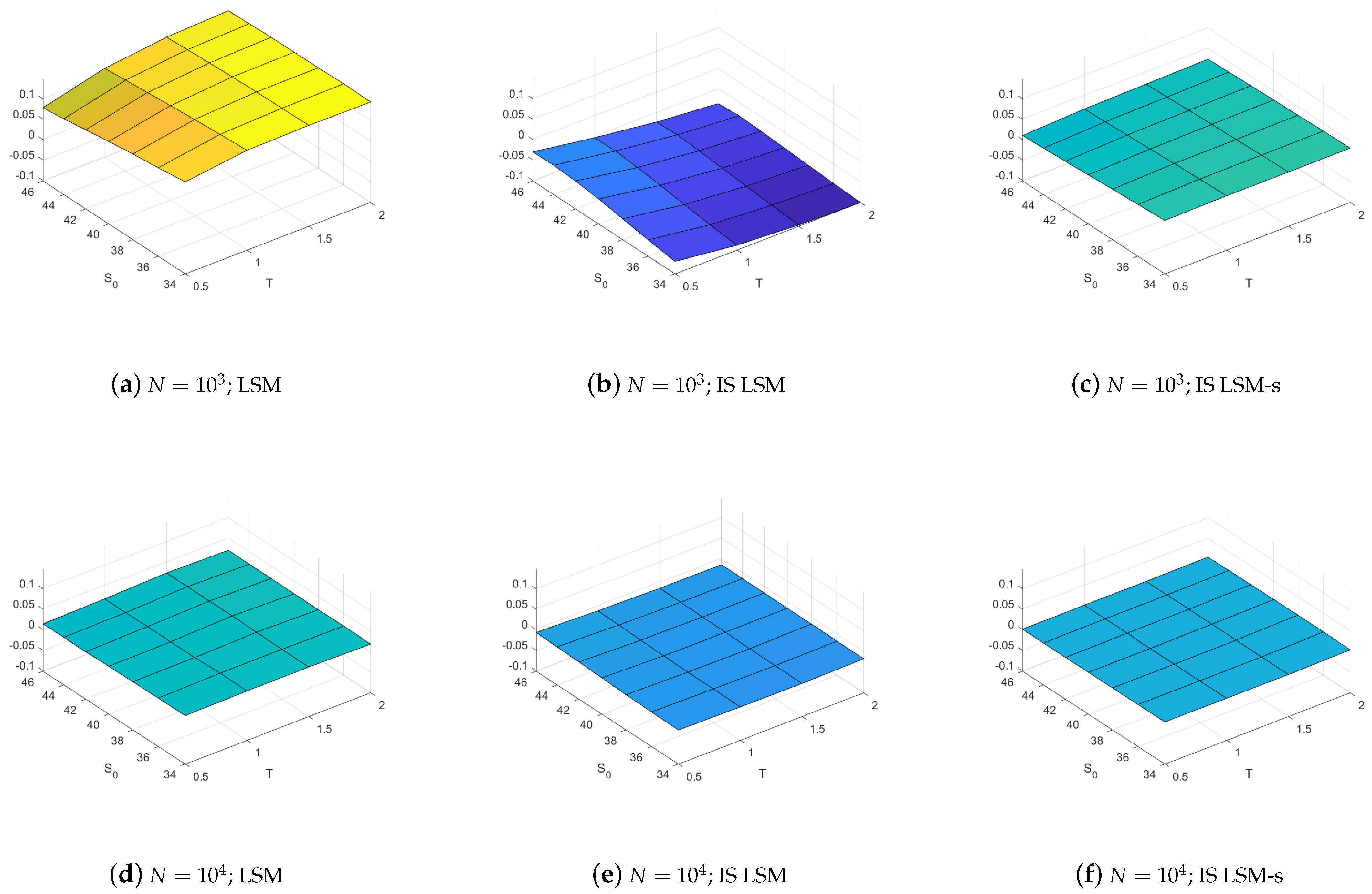
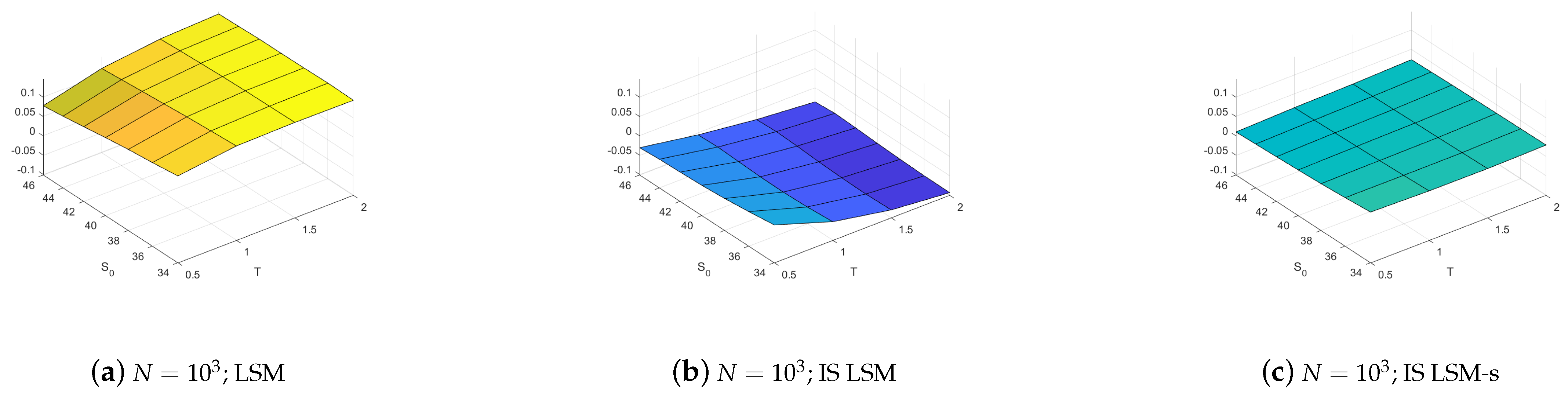
We first note from Figure 2 that the LSM-s estimators always have the smallest bias.4 Indeed, a significant bias is observed when importance sampling is used with the LSM, IS LSM, but this bias is eliminated with the importance sample LSM-s, IS LSM-s, even when as little as paths are used in the simulation. The LSM-s also has smaller bias than the LSM with and without importance sampling for all 28 options when using paths, although the magnitude of the bias tends to be smaller. The detailed results in Table A1 in Appendix A shows that this pattern persists when a large sample of paths is used in the simulation although in this case the size of the bias is essentially negligible. From these results we conclude that the LSM-s offers important reductions in the estimator bias compared to the LSM counterparts with and without importance sampling, and this is particularly so when the number of simulation paths is low.
The results in Figure 2 demonstrate that fitted regression values tend to be less accurate when regression coefficients estimated under the nominal measure are used to estimate continuation values when conditioning on values simulated from the importance measure. Indeed, continuation values can be difficult to approximate, especially if they take the form of a polynomial extrapolation for deep ITM paths. By regressing on paths from the importance measure the fitted values are more robust for deep ITM paths. Having a larger sample of deep ITM paths also contributes to preserving the convexity of continuation values with respect to the asset price. This effect reduces the frequency and importance of exercise errors and thus corrects the bias.
3.2.2. Standard Deviation
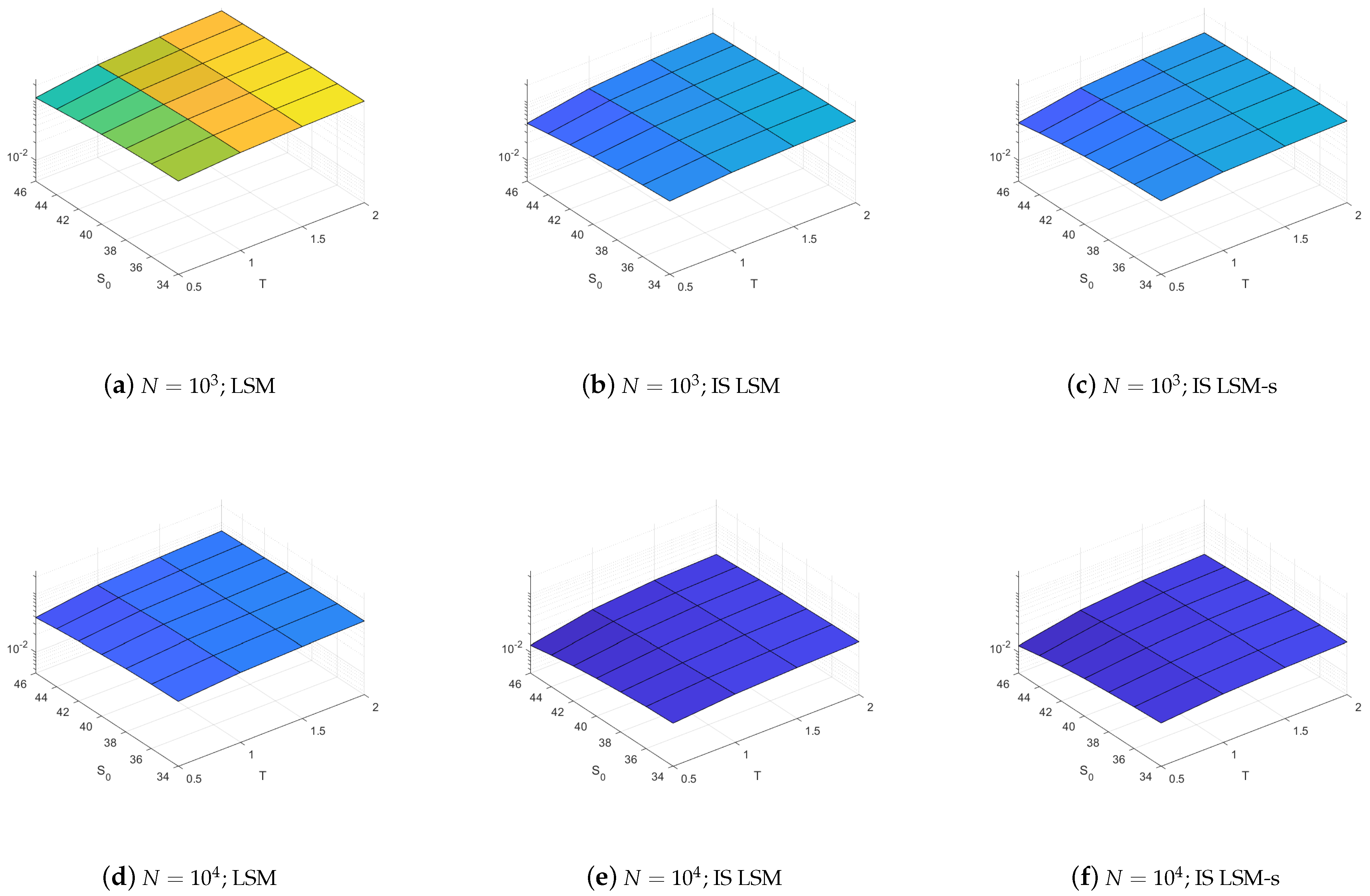
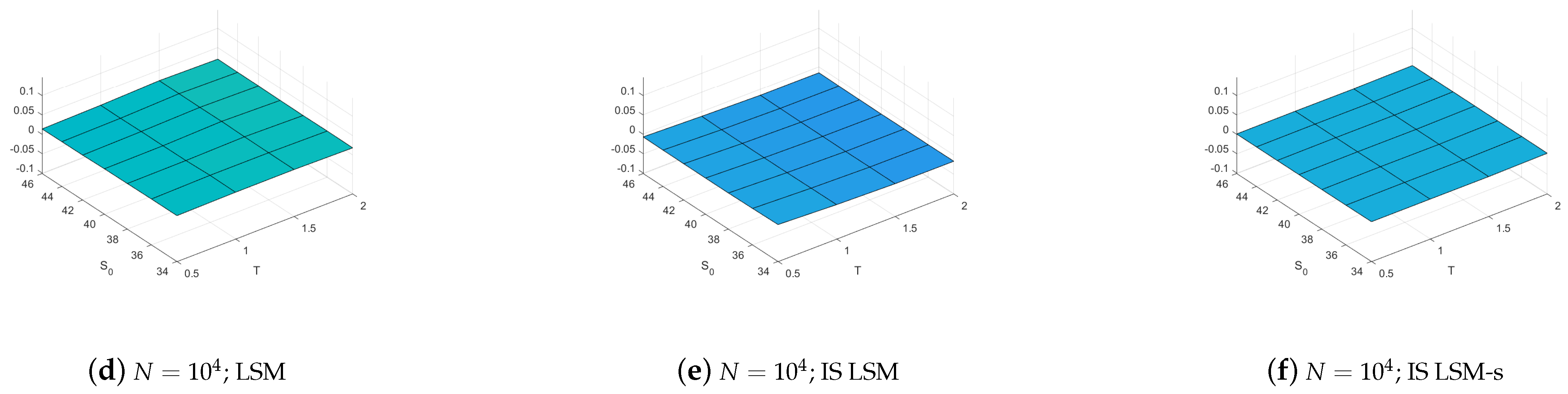
We next note from Figure 3 that the importance sampling variance reductions of the LSM and LSM-s estimators are remarkably similar. This is also confirmed by the detailed results shown in Table A3 in Appendix A. The figure also shows that compared to the variance of the LSM estimator without importance sampling the standard deviations are significantly lower, often around half of what is obtained without importance sampling, and importance sampling is, thus, clearly effective as a variance reduction technique.
The results in Figure 3 demonstrates that while the estimated early exercise strategy is worse with the IS LSM than when using the IS LSM-s it is “equally” suboptimal across all repetitions leading to an estimator bias of similar size. Once an early exercise strategy has been estimated, valuing the option amounts to averaging discounted payoffs and the fraction of such payoffs that are non-zero depends much less on the estimated exercise strategy and much more on the change of measure.
3.2.3. RMSE Efficiency
The results above demonstrate the efficiency of importance sampling as a variance reduction technique. They also demonstrate that the standard implementation may introduce a significant bias in the estimator which fortunately can be eliminated by using our proposed shifted LSM regression methodology. Combining these two findings we expect the root mean squared error, RMSE, of the estimated prices to be smaller when using LSM-s than when using LSM with importance sampling. We also expect that both methods have RMSEs that are much smaller than what is obtained with the LSM method implemented without any importance sampling. To illustrate this in a more concise way, we compute the RMSE efficiency of a given estimator as
In other words, the efficiencies of importance sampling for the LSM and the LSM-s are measured relative to the standard LSM estimator with the same number of paths.
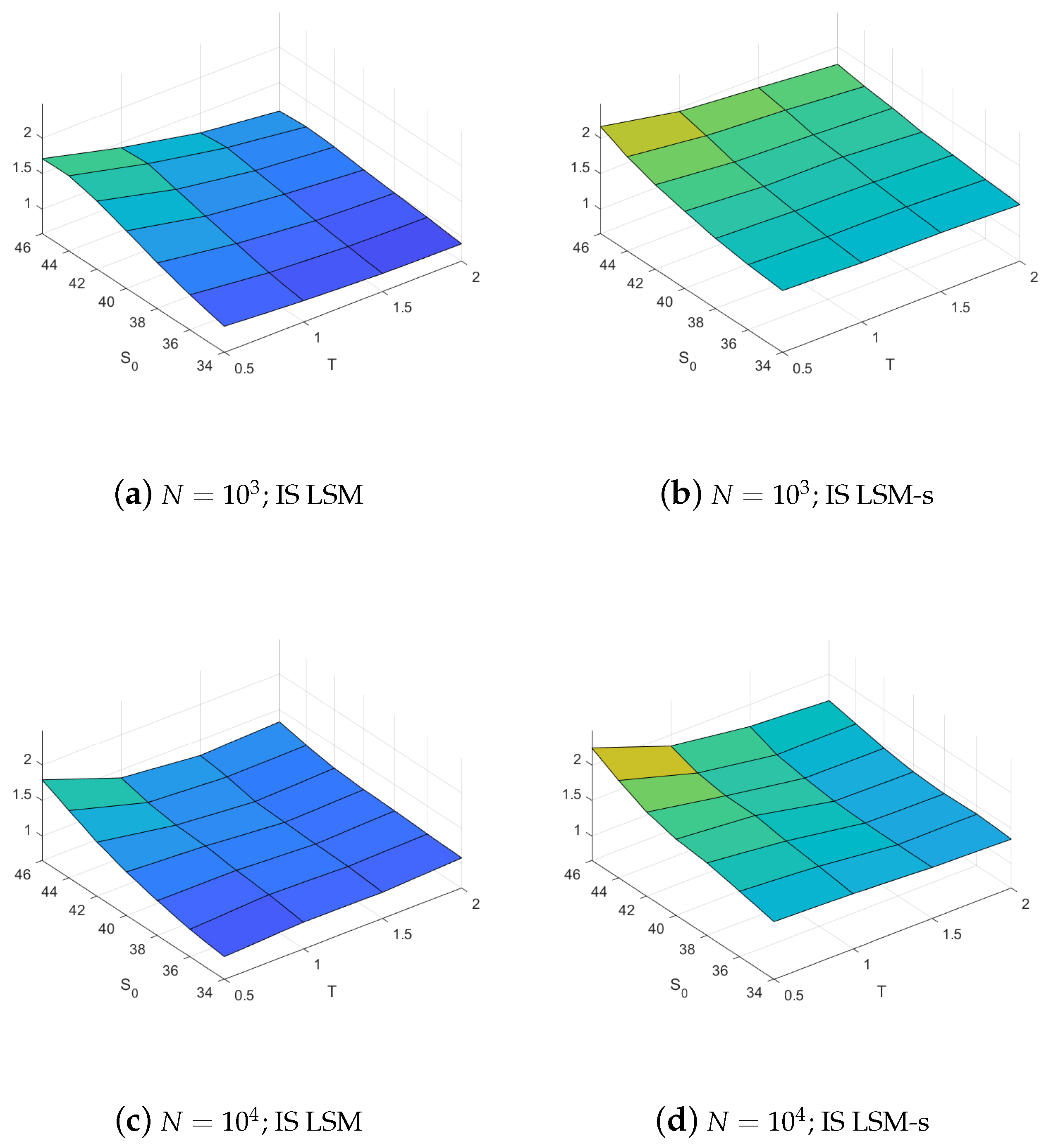
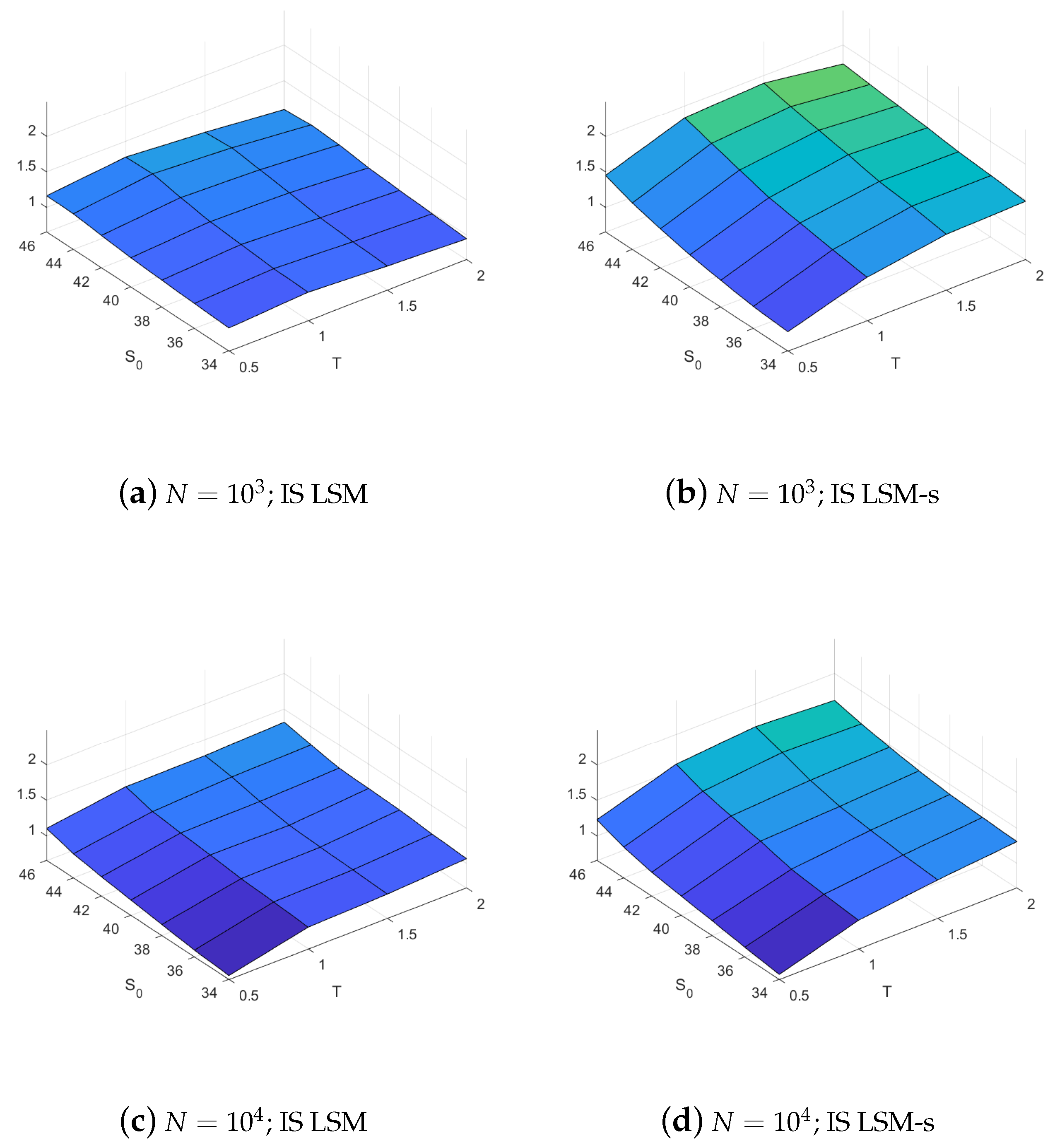
Figure 4 plots the efficiencies for the two methods and demonstrates that the LSM-s method indeed has the highest RMSE efficiency across the board for all the options, and this holds irrespective of the number of paths used. When using only paths the average efficiency of the LSM-s is an impressive . The RMSE of the IS LSM-s is on average smaller than that of the IS LSM, at least better and could improve on the IS LSM by as much as . The detailed results in Table A5 in Appendix A shows that the LSM-s also exhibits higher efficiencies when a large sample of paths is used in the simulation. However, the relative difference between the efficiencies of importance sampling for LSM and LSM-s methods decreases with the sample size because the bias improvement is negligible.
The results in the above figures therefore provide strong support for our proposed method. In particular, they demonstrate that our proposed method should be particularly useful when one is restricted to using a low number of simulated paths for option pricing. Moreover, because of the reduced bias this method lends itself to simple parallel implementation where many independent jobs (with small sample size) are serially farmed out to processors in parallel. The reduction in bias allows for more accurate estimators when computing price estimators in this fashion as compared to the LSM and IS LSM estimators, respectively.
3.3. Robustness
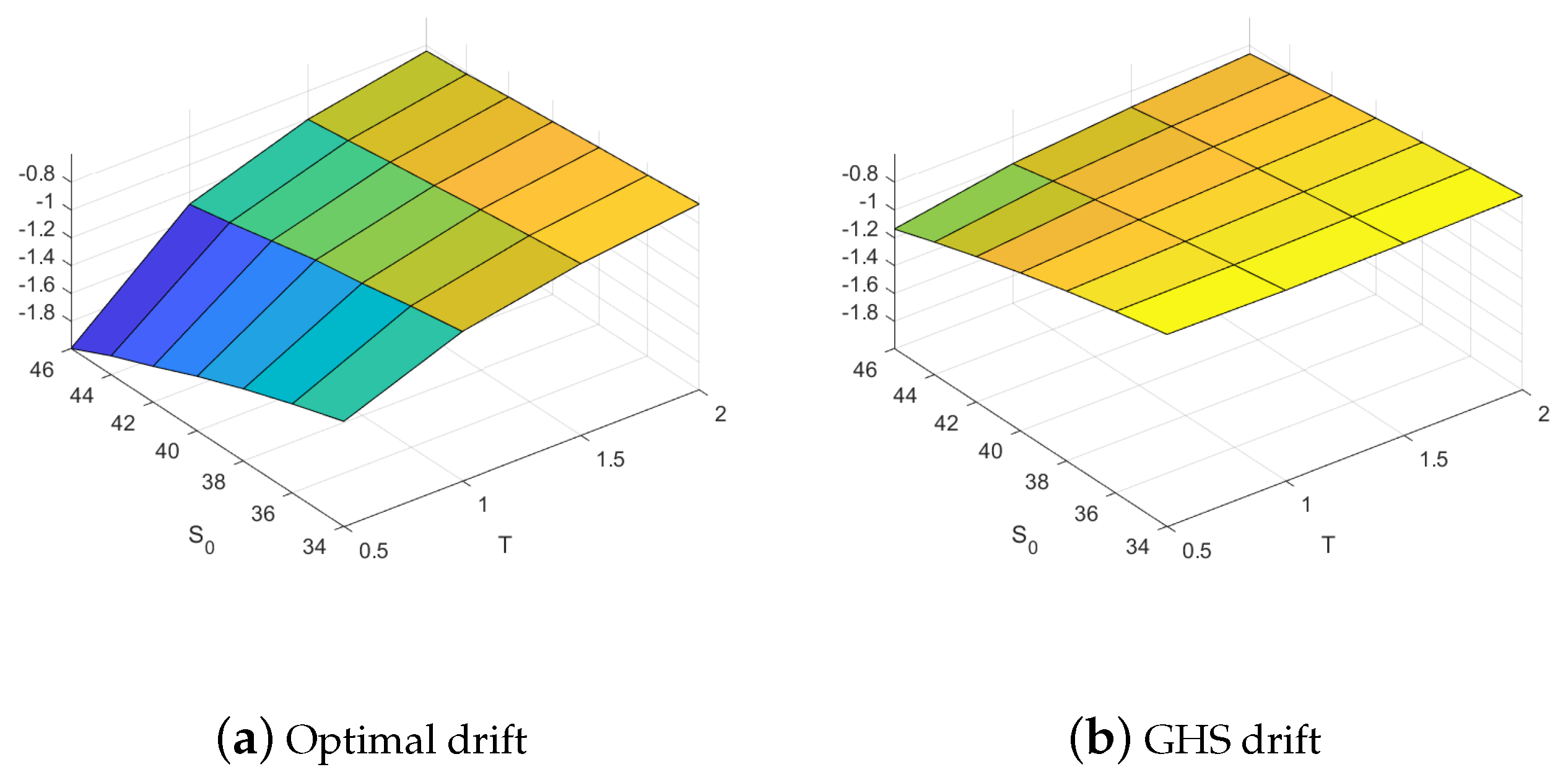
The results in Section 3.2 are based on the optimal (but potentially infeasible) drift which is difficult (or even impossible) to calculate as it requires knowledge of the optimal early exercise strategy. In this section we, therefore, consider the robustness of our results when the easier to calculate but suboptimal GHS change of drift is used. Figure 5 demonstrates that the changes of drift indeed differ and that it tends to be much smaller for the suboptimal GHS method and this particularly so for short maturity options.
Figure 6, Figure 7 and Figure 8 show the bias, standard deviation and RMSE efficiencies when the GHS drift is used. The corresponding detailed results are found in Table A2, Table A4 and Table A6 in Appendix A. These plots look very similar to what is obtained with an optimal drift. In particular, Figure 6 shows that the LSM-s has the smallest bias in the vast majority of the cases, although the bias is slightly smaller with the IS LSM for the 3 out of the money short term options when paths are used, Figure 7 shows that the standard deviations of the IS LSM and IS LSM-s are very close and much smaller than the LSM without importance sampling, and Figure 8 shows that as a result the IS LSM-s is significantly more efficient than the IS LSM when measured with RMSE.
When using paths only, with the GHS drift the average efficiency of the IS LSM-s is still large at and the RMSE of the IS LSM-s is on average smaller than that of the IS LSM. These results, therefore, demonstrate that our proposed method is indeed robust to the choice of (optimal) change of drift and hold true even when a suboptimal change of drift is considered. Moreover, the results confirm that our proposed method should be particularly useful when one is restricted to using a low number of simulated paths for option pricing.
4. Extensions and Future Research
Importance sampling can be extended to a multivariate setting as in Moreni (2004). In particular, we can model D correlated GBM processes as a vector with a vector of continuously compounded dividend yields , and a positive definite covariance matrix , where A is a lower-triangular matrix and C is a diagonal matrix.5 Discretized paths are simulated under the nominal measure with
where is a vector of independent normal increments, and is a vector of mean log-returns defined as the difference between the continuously compounded risk-free rate and asset-specific dividend yield. Paths are simulated under the importance measure with the drift adjustment by using the same multivariate normal increments to generate . Under both measures the initial values of each path are the same, , and path are simulated under the importance measure with
The k-step likelihood ratio for the discretized multivariate diffusion process takes the form
for any and . One can then optimize the importance drift with a gradient descent routine or use the saddle point approximation of Glasserman et al. (1999) when a closed-form solution to the analogous European-style option price is available.
In addition to the multivariate generalizations, it may also be desirable to consider importance sampling in models with fat-tailed distributions and variance dynamics for the underlying assets as exhibited in financial time series. When it comes to accommodating non-Gaussian fat-tailed returns, it is important to note that importance sampling techniques are not at all restricted to GBMs, as they only require that the importance distribution be absolutely continuous with respect to the nominal distribution. In such cases, the Radon–Nikodym derivative is well defined, and if it can be computed in a cost-effective way, importance sampling yields appreciable variance reduction for security pricing (see Boyle et al. (1997)). When it come to allowing for more flexible variance dynamics, Glasserman et al. (1999) also note that their approach can be used with the Hull and White (1987) stochastic volatility model or the Cox et al. (1977) mean-reverting square-root volatility model for interest rate derivatives.6 For all these cases, the optimization of the drift term can be carried out with a gradient descent for any model specification or option payoff (Su and Fu 2000).
The shifted regression method proposed herein for American options can in principle be used with (all combinations of) the extensions outlined above simply by adjusting the likelihood ratio accordingly. Extensions to the multivariate setting are particular straightforward and simple to implement. However, to our knowledge applications of importance sampling for American option pricing in the presence of stochastic volatility and conditional heteroskedasticity (i.e., GARCH-type models) has yet to be thoroughly examined in the literature. The extension to the class of GARCH models, in particular with fat-tailed conditional distributions, is particularly interesting and challenging and it is currently the subject of ongoing research.7
5. Conclusions
This paper proposes a new method for pricing American options when using importance sampling as a variance reduction technique in simulation-and-regression based methods. Our suggested method uses regressions under the importance measure directly to determine the optimal early exercise strategy. The standard method for using importance sampling is instead to use regressions under the nominal measure.
We show that our proposed method offers several important benefits. First, our proposed method requires no prior knowledge of regression coefficients since the regressions are carried out directly with the importance paths and our approach, therefore, removes the overhead related to estimating an exercise strategy under the nominal measure. Second, our proposed method successfully reduces the bias that plague the standard LSM method with and without importance sampling by improving the accuracy of an exercise strategy. Third, the shifted LSM approach preserves the variance reduction in the standard implementation of importance sampling.
As a result, when a low number of paths is used, our method always improves on the standard method and reduces average root means squared error of estimated option prices by . Hence, the Monte Carlo valuation of deep out of the money options, knock-in options or barrier options with American-style features may greatly benefit from the approach introduced in this paper. Moreover, our methods lends itself to simple parallel implementation where many independent jobs (with small sample size) are serially farmed out to processors in parallel because of the reduced bias compared to standard (and unshifted) estimators.
Author Contributions
Conceptualization, F.-M.B., R.M.R. and L.S.; data curation, F.-M.B. and R.M.R.; formal analysis, F.-M.B. and R.M.R.; funding acquisition, F.-M.B. and R.M.R.; project administration, L.S.; supervision, L.S. All authors have read and agreed to the published version of the manuscript.
Funding
F.-M. Boire thanks the University of Western Ontario and OGS for financial support. M. Reesor thanks NSERC and Wilfrid Laurier University for financial support. L. Stentoft thanks NSERC for financial support.
Institutional Review Board Statement
Not applicable.
Informed Consent Statement
Not applicable.
Data Availability Statement
Data sharing is not applicable to this article.
Acknowledgments
The authors would like to thank three anonymous referees for valuable comments and SHARCNET for providing computational resources.
Conflicts of Interest
The authors declare no conflict of interest.
Appendix A. Tables with Detailed Results
This appendix provides detailed results for the performance of the various methods used in this paper under the two different choices of change of measures used. Table A1 and Table A2 present bias results, calculated with respect to a Cox et al. (1979) binomial tree solution, for the LSM, IS LSM, and IS LSM-s estimators across the 28 options considered for different number of paths and repetitions with the optimal drift and GHS approximate drift, respectively. Table A3, Table A4, Table A5 and Table A6 present corresponding results for the standard deviation and root mean squared error, RMSE, respectively.

Table A1.
Detailed bias results () with optimized drift.
| 0.5 | 34 | 117.1 | −73.3 | 28.5 | 17.6 | −18.9 | 1.7 | −2.3 | −4.6 | −2.0 |
| 0.5 | 36 | 110.1 | −62.7 | 24.1 | 15.8 | −17.8 | 1.5 | −3.1 | −3.8 | −1.4 |
| 0.5 | 38 | 104.2 | −52.1 | 21.5 | 14.4 | −15.5 | 3.0 | −1.2 | −5.8 | −0.9 |
| 0.5 | 40 | 95.0 | −42.1 | 17.6 | 15.9 | −12.8 | 2.1 | −0.0 | −3.9 | −1.5 |
| 0.5 | 42 | 90.9 | −33.8 | 15.3 | 14.1 | −11.0 | 2.1 | −1.0 | −3.3 | −0.7 |
| 0.5 | 44 | 81.4 | −30.0 | 12.2 | 15.4 | −7.8 | 1.1 | 0.6 | −3.9 | −0.4 |
| 0.5 | 46 | 75.4 | −30.2 | 9.1 | 12.0 | −6.6 | 0.5 | −1.2 | −2.3 | −1.1 |
| 1 | 34 | 138.5 | −91.5 | 30.1 | 21.3 | −19.6 | 0.1 | 4.6 | −3.9 | −2.3 |
| 1 | 36 | 138.6 | −81.6 | 26.6 | 17.8 | −18.8 | 2.4 | −2.4 | −6.4 | −0.8 |
| 1 | 38 | 132.0 | −74.2 | 25.4 | 15.1 | −16.6 | 2.4 | −3.3 | −4.1 | −1.1 |
| 1 | 40 | 128.1 | −66.4 | 22.0 | 15.4 | −15.5 | 1.5 | 1.6 | −4.7 | −1.0 |
| 1 | 42 | 124.4 | −60.4 | 19.7 | 20.5 | −17.0 | 2.4 | 2.7 | −4.3 | −0.9 |
| 1 | 44 | 118.7 | −54.2 | 17.1 | 17.9 | −12.6 | 1.5 | −2.4 | −3.8 | −0.8 |
| 1 | 46 | 114.6 | −54.9 | 15.8 | 18.4 | −11.9 | 2.0 | 3.5 | −4.3 | 0.3 |
| 1.5 | 34 | 141.5 | −99.5 | 31.5 | 20.0 | −20.7 | 3.4 | −1.3 | −4.4 | −0.1 |
| 1.5 | 36 | 141.2 | −93.2 | 29.2 | 22.5 | −19.4 | 0.9 | −0.1 | −5.2 | −1.8 |
| 1.5 | 38 | 141.9 | −89.7 | 27.1 | 18.7 | −18.6 | 3.6 | −0.2 | −5.3 | −1.9 |
| 1.5 | 40 | 138.3 | −82.4 | 24.8 | 13.7 | −18.2 | 2.1 | −0.1 | −4.0 | −0.3 |
| 1.5 | 42 | 134.2 | −76.1 | 23.4 | 15.5 | −15.8 | 2.4 | 0.9 | −4.8 | 0.3 |
| 1.5 | 44 | 131.7 | −72.6 | 20.0 | 15.2 | −16.4 | 2.4 | −0.5 | −3.4 | −1.7 |
| 1.5 | 46 | 129.2 | −74.3 | 18.9 | 15.6 | −14.3 | 1.7 | −1.0 | −4.0 | −1.3 |
| 2 | 34 | 141.8 | −104.3 | 30.6 | 16.7 | −20.9 | 1.7 | 0.7 | −4.5 | −2.2 |
| 2 | 36 | 144.0 | −98.8 | 29.0 | 13.1 | −20.4 | 1.9 | −1.0 | −4.2 | −2.1 |
| 2 | 38 | 142.0 | −95.7 | 26.0 | 17.2 | −17.5 | 2.4 | −0.1 | −4.1 | −0.8 |
| 2 | 40 | 141.0 | −91.8 | 24.8 | 14.5 | −18.3 | 1.8 | −1.1 | −5.6 | −1.7 |
| 2 | 42 | 139.4 | −87.1 | 27.0 | 18.7 | −17.9 | 2.3 | 5.3 | −4.4 | −1.4 |
| 2 | 44 | 141.6 | −84.5 | 23.2 | 17.0 | −18.5 | 3.1 | 3.2 | −4.2 | −1.2 |
| 2 | 46 | 137.6 | −87.9 | 21.8 | 19.2 | −16.8 | 1.1 | 1.3 | −2.9 | −0.7 |
Table A2.
Detailed bias results () with GHS drift.
| 0.5 | 34 | 117.1 | −3.0 | 26.7 | 17.6 | −5.8 | 1.3 | −2.3 | −3.1 | −2.2 |
| 0.5 | 36 | 110.1 | −11.8 | 21.8 | 15.8 | −7.2 | 2.1 | −3.1 | −3.5 | −2.4 |
| 0.5 | 38 | 104.2 | −20.3 | 18.7 | 14.4 | −8.1 | 0.6 | −1.2 | −1.5 | −2.0 |
| 0.5 | 40 | 95.0 | −25.2 | 15.4 | 15.9 | −8.9 | −0.2 | −0.0 | −2.0 | −1.5 |
| 0.5 | 42 | 90.9 | −26.4 | 13.2 | 14.1 | −8.5 | −0.2 | −1.0 | −3.1 | −2.2 |
| 0.5 | 44 | 81.4 | −28.6 | 10.2 | 15.4 | −8.0 | 0.6 | 0.6 | −3.0 | −1.4 |
| 0.5 | 46 | 75.4 | −32.2 | 8.9 | 12.0 | −7.4 | 0.4 | −1.2 | −2.8 | −0.9 |
| 1 | 34 | 138.5 | −56.7 | 23.8 | 21.3 | −14.5 | −0.2 | 4.6 | −2.3 | −0.6 |
| 1 | 36 | 138.6 | −59.7 | 22.2 | 17.8 | −13.2 | 0.5 | −2.4 | −1.9 | −0.7 |
| 1 | 38 | 132.0 | −59.7 | 21.2 | 15.1 | −13.5 | 1.6 | −3.3 | −5.0 | −1.0 |
| 1 | 40 | 128.1 | −61.3 | 18.9 | 15.4 | −14.7 | 0.2 | 1.6 | −3.7 | 0.1 |
| 1 | 42 | 124.4 | −58.5 | 17.1 | 20.5 | −12.5 | 0.7 | 2.7 | −2.3 | −1.4 |
| 1 | 44 | 118.7 | −54.8 | 14.7 | 17.9 | −14.0 | 0.1 | −2.4 | −2.5 | −1.8 |
| 1 | 46 | 114.6 | −57.2 | 14.8 | 18.4 | −13.4 | 1.5 | 3.5 | −3.8 | −0.4 |
| 1.5 | 34 | 141.5 | −81.4 | 23.1 | 20.0 | −15.6 | 0.5 | −1.3 | −4.6 | −0.6 |
| 1.5 | 36 | 141.2 | −85.0 | 23.5 | 22.5 | −16.4 | 1.4 | −0.1 | −3.6 | −1.5 |
| 1.5 | 38 | 141.9 | −83.5 | 22.0 | 18.7 | −16.7 | 3.7 | −0.2 | −4.0 | −2.6 |
| 1.5 | 40 | 138.3 | −80.4 | 21.6 | 13.7 | −19.0 | 1.0 | −0.1 | −4.1 | −2.1 |
| 1.5 | 42 | 134.2 | −76.1 | 19.1 | 15.5 | −17.0 | 1.7 | 0.9 | −6.1 | −1.8 |
| 1.5 | 44 | 131.7 | −73.0 | 18.3 | 15.2 | −15.7 | 3.1 | −0.5 | −4.3 | −1.7 |
| 1.5 | 46 | 129.2 | −75.4 | 17.8 | 15.6 | −15.2 | 2.0 | −1.0 | −2.7 | −1.6 |
| 2 | 34 | 141.8 | −95.2 | 27.0 | 16.7 | −21.4 | 1.8 | 0.7 | −0.4 | −2.9 |
| 2 | 36 | 144.0 | −96.1 | 27.3 | 13.1 | −18.8 | 3.6 | −1.0 | −6.6 | −1.5 |
| 2 | 38 | 142.0 | −94.0 | 27.0 | 17.2 | −17.7 | 1.7 | −0.1 | −4.4 | −4.8 |
| 2 | 40 | 141.0 | −91.1 | 24.7 | 14.5 | −17.2 | 3.5 | −1.1 | −5.3 | −1.4 |
| 2 | 42 | 139.4 | −87.7 | 25.5 | 18.7 | −18.3 | 2.1 | 5.3 | −3.9 | −1.1 |
| 2 | 44 | 141.6 | −84.6 | 23.8 | 17.0 | −16.1 | 3.7 | 3.2 | −3.3 | −0.7 |
| 2 | 46 | 137.6 | −89.2 | 21.7 | 19.2 | −15.7 | 2.5 | 1.3 | −3.6 | 0.4 |
Table A3.
Detailed standard deviation results () with optimized drift.
| 0.5 | 34 | 18.2 | 8.1 | 8.1 | 5.7 | 2.5 | 2.5 | 1.7 | 0.8 | 0.9 |
| 0.5 | 36 | 17.6 | 7.5 | 7.7 | 5.6 | 2.2 | 2.4 | 1.5 | 0.7 | 0.8 |
| 0.5 | 38 | 16.8 | 7.0 | 7.2 | 5.5 | 2.2 | 2.1 | 1.7 | 0.6 | 0.7 |
| 0.5 | 40 | 15.9 | 6.3 | 6.5 | 4.9 | 1.9 | 2.0 | 1.4 | 0.7 | 0.7 |
| 0.5 | 42 | 14.7 | 5.7 | 5.9 | 4.8 | 1.8 | 1.9 | 1.3 | 0.5 | 0.6 |
| 0.5 | 44 | 13.4 | 4.9 | 5.1 | 4.4 | 1.6 | 1.5 | 1.4 | 0.5 | 0.4 |
| 0.5 | 46 | 12.2 | 4.3 | 4.5 | 3.9 | 1.3 | 1.3 | 1.4 | 0.4 | 0.4 |
| 1 | 34 | 21.6 | 10.0 | 9.9 | 6.6 | 3.0 | 3.0 | 2.3 | 0.8 | 1.0 |
| 1 | 36 | 21.2 | 9.4 | 9.4 | 6.6 | 2.9 | 2.9 | 2.0 | 0.9 | 0.9 |
| 1 | 38 | 21.1 | 8.9 | 9.1 | 6.6 | 2.9 | 2.9 | 2.2 | 0.9 | 0.9 |
| 1 | 40 | 20.4 | 8.4 | 8.7 | 6.4 | 2.6 | 2.5 | 1.8 | 0.9 | 0.8 |
| 1 | 42 | 19.4 | 7.9 | 8.1 | 6.3 | 2.5 | 2.5 | 1.8 | 0.8 | 0.8 |
| 1 | 44 | 18.3 | 7.3 | 7.5 | 6.0 | 2.2 | 2.3 | 1.9 | 0.6 | 0.7 |
| 1 | 46 | 17.4 | 6.7 | 6.9 | 5.6 | 2.1 | 2.1 | 1.8 | 0.6 | 0.7 |
| 1.5 | 34 | 23.6 | 10.8 | 10.9 | 7.8 | 3.2 | 3.3 | 2.2 | 1.0 | 1.1 |
| 1.5 | 36 | 23.6 | 10.6 | 10.5 | 7.8 | 3.2 | 3.3 | 2.2 | 1.1 | 1.1 |
| 1.5 | 38 | 23.1 | 10.1 | 10.1 | 7.6 | 3.1 | 3.1 | 2.1 | 1.0 | 1.0 |
| 1.5 | 40 | 22.5 | 9.7 | 9.8 | 7.1 | 2.9 | 3.1 | 2.3 | 0.9 | 0.9 |
| 1.5 | 42 | 22.0 | 9.3 | 9.4 | 6.9 | 2.9 | 2.9 | 2.2 | 0.8 | 0.9 |
| 1.5 | 44 | 21.3 | 8.8 | 9.0 | 6.8 | 2.6 | 2.7 | 2.1 | 0.7 | 0.9 |
| 1.5 | 46 | 20.7 | 8.3 | 8.5 | 6.5 | 2.5 | 2.5 | 2.1 | 0.8 | 0.7 |
| 2 | 34 | 25.2 | 11.4 | 11.4 | 8.0 | 3.5 | 3.5 | 2.6 | 1.0 | 1.2 |
| 2 | 36 | 25.1 | 11.3 | 11.3 | 8.1 | 3.5 | 3.5 | 2.3 | 1.0 | 1.1 |
| 2 | 38 | 24.7 | 10.9 | 11.1 | 7.4 | 3.4 | 3.4 | 2.4 | 1.0 | 1.1 |
| 2 | 40 | 24.5 | 10.5 | 10.6 | 7.6 | 3.3 | 3.2 | 2.3 | 1.1 | 1.0 |
| 2 | 42 | 24.2 | 10.2 | 10.2 | 7.6 | 3.0 | 3.1 | 2.2 | 0.9 | 1.1 |
| 2 | 44 | 23.2 | 9.7 | 9.9 | 7.2 | 2.9 | 3.0 | 2.3 | 0.9 | 0.9 |
| 2 | 46 | 22.6 | 9.3 | 9.4 | 7.1 | 2.8 | 2.8 | 2.1 | 0.9 | 0.9 |
Table A4.
Detailed standard deviation results () with GHS drift.
| 0.5 | 34 | 18.2 | 10.9 | 10.9 | 5.7 | 3.6 | 3.6 | 1.7 | 1.2 | 1.1 |
| 0.5 | 36 | 17.6 | 10.4 | 10.3 | 5.6 | 3.2 | 3.2 | 1.5 | 1.0 | 1.0 |
| 0.5 | 38 | 16.8 | 9.4 | 9.5 | 5.5 | 2.9 | 3.0 | 1.7 | 0.8 | 0.9 |
| 0.5 | 40 | 15.9 | 8.7 | 8.6 | 4.9 | 2.7 | 2.7 | 1.4 | 0.8 | 0.9 |
| 0.5 | 42 | 14.7 | 7.7 | 7.7 | 4.8 | 2.4 | 2.3 | 1.3 | 0.8 | 0.8 |
| 0.5 | 44 | 13.4 | 6.7 | 6.7 | 4.4 | 2.1 | 2.1 | 1.4 | 0.6 | 0.7 |
| 0.5 | 46 | 12.2 | 5.9 | 5.8 | 3.9 | 1.8 | 1.9 | 1.4 | 0.6 | 0.6 |
| 1 | 34 | 21.6 | 11.5 | 11.2 | 6.6 | 3.4 | 3.7 | 2.3 | 1.1 | 1.1 |
| 1 | 36 | 21.2 | 10.9 | 10.8 | 6.6 | 3.3 | 3.5 | 2.0 | 0.9 | 0.9 |
| 1 | 38 | 21.1 | 10.2 | 10.1 | 6.6 | 3.2 | 3.1 | 2.2 | 0.9 | 0.8 |
| 1 | 40 | 20.4 | 9.5 | 9.3 | 6.4 | 3.0 | 2.9 | 1.8 | 1.0 | 1.0 |
| 1 | 42 | 19.4 | 8.7 | 8.6 | 6.3 | 2.7 | 2.8 | 1.8 | 0.7 | 0.8 |
| 1 | 44 | 18.3 | 8.0 | 8.0 | 6.0 | 2.5 | 2.6 | 1.9 | 0.8 | 0.8 |
| 1 | 46 | 17.4 | 7.3 | 7.3 | 5.6 | 2.3 | 2.3 | 1.8 | 0.7 | 0.7 |
| 1.5 | 34 | 23.6 | 11.6 | 11.2 | 7.8 | 3.7 | 3.7 | 2.2 | 1.1 | 1.0 |
| 1.5 | 36 | 23.6 | 11.2 | 10.8 | 7.8 | 3.3 | 3.3 | 2.2 | 1.1 | 1.0 |
| 1.5 | 38 | 23.1 | 10.5 | 10.4 | 7.6 | 3.2 | 3.3 | 2.1 | 1.0 | 0.9 |
| 1.5 | 40 | 22.5 | 9.9 | 9.7 | 7.1 | 3.1 | 3.1 | 2.3 | 1.0 | 0.9 |
| 1.5 | 42 | 22.0 | 9.5 | 9.4 | 6.9 | 2.9 | 2.9 | 2.2 | 1.0 | 0.9 |
| 1.5 | 44 | 21.3 | 8.9 | 8.9 | 6.8 | 2.6 | 2.7 | 2.1 | 1.0 | 0.8 |
| 1.5 | 46 | 20.7 | 8.5 | 8.3 | 6.5 | 2.6 | 2.6 | 2.1 | 0.9 | 0.8 |
| 2 | 34 | 25.2 | 11.6 | 11.3 | 8.0 | 3.6 | 3.7 | 2.6 | 1.0 | 1.1 |
| 2 | 36 | 25.1 | 11.2 | 11.0 | 8.1 | 3.4 | 3.4 | 2.3 | 1.2 | 1.1 |
| 2 | 38 | 24.7 | 11.0 | 10.7 | 7.4 | 3.5 | 3.4 | 2.4 | 1.2 | 1.1 |
| 2 | 40 | 24.5 | 10.5 | 10.5 | 7.6 | 3.3 | 3.2 | 2.3 | 1.0 | 0.9 |
| 2 | 42 | 24.2 | 10.1 | 10.2 | 7.6 | 3.1 | 3.2 | 2.2 | 0.9 | 1.0 |
| 2 | 44 | 23.2 | 9.8 | 10.1 | 7.2 | 3.1 | 2.9 | 2.3 | 0.8 | 1.0 |
| 2 | 46 | 22.6 | 9.5 | 9.5 | 7.1 | 3.0 | 2.7 | 2.1 | 0.9 | 0.9 |
Table A5.
Detailed RMSE efficiency results with optimized drift.
| 0.5 | 34 | 0.98 | 1.52 | 0.90 | 1.43 | 0.81 | 0.95 |
| 0.5 | 36 | 1.12 | 1.56 | 1.05 | 1.42 | 0.99 | 1.05 |
| 0.5 | 38 | 1.28 | 1.64 | 1.13 | 1.63 | 0.94 | 1.39 |
| 0.5 | 40 | 1.43 | 1.73 | 1.22 | 1.55 | 0.86 | 1.10 |
| 0.5 | 42 | 1.61 | 1.85 | 1.39 | 1.64 | 1.29 | 1.29 |
| 0.5 | 44 | 1.71 | 1.98 | 1.63 | 2.13 | 1.18 | 2.10 |
| 0.5 | 46 | 1.72 | 2.13 | 1.71 | 2.13 | 2.03 | 2.34 |
| 1 | 34 | 0.89 | 1.48 | 0.94 | 1.30 | 1.50 | 1.33 |
| 1 | 36 | 1.03 | 1.59 | 0.97 | 1.34 | 0.80 | 1.21 |
| 1 | 38 | 1.15 | 1.63 | 1.05 | 1.36 | 1.18 | 1.41 |
| 1 | 40 | 1.25 | 1.68 | 1.15 | 1.57 | 0.77 | 1.13 |
| 1 | 42 | 1.32 | 1.76 | 1.17 | 1.66 | 0.94 | 1.33 |
| 1 | 44 | 1.40 | 1.83 | 1.49 | 1.69 | 1.55 | 1.83 |
| 1 | 46 | 1.40 | 1.94 | 1.46 | 1.83 | 1.41 | 1.72 |
| 1.5 | 34 | 0.87 | 1.43 | 1.09 | 1.42 | 0.97 | 1.09 |
| 1.5 | 36 | 0.95 | 1.53 | 1.16 | 1.46 | 0.89 | 0.94 |
| 1.5 | 38 | 1.00 | 1.58 | 1.17 | 1.49 | 0.86 | 0.99 |
| 1.5 | 40 | 1.07 | 1.61 | 1.12 | 1.31 | 1.23 | 1.44 |
| 1.5 | 42 | 1.14 | 1.67 | 1.13 | 1.48 | 1.24 | 1.33 |
| 1.5 | 44 | 1.19 | 1.72 | 1.25 | 1.56 | 1.58 | 1.29 |
| 1.5 | 46 | 1.19 | 1.79 | 1.37 | 1.69 | 1.39 | 1.98 |
| 2 | 34 | 0.88 | 1.46 | 1.01 | 1.34 | 1.36 | 1.06 |
| 2 | 36 | 0.93 | 1.48 | 1.04 | 1.35 | 1.13 | 0.94 |
| 2 | 38 | 0.96 | 1.50 | 0.99 | 1.27 | 1.17 | 1.29 |
| 2 | 40 | 1.02 | 1.59 | 1.06 | 1.44 | 0.88 | 1.31 |
| 2 | 42 | 1.08 | 1.64 | 1.26 | 1.55 | 1.27 | 1.08 |
| 2 | 44 | 1.12 | 1.68 | 1.16 | 1.44 | 1.39 | 1.46 |
| 2 | 46 | 1.07 | 1.75 | 1.27 | 1.63 | 1.31 | 1.40 |
Table A6.
Detailed RMSE efficiency results with GHS drift.
| 0.5 | 34 | 0.98 | 0.93 | 0.65 | 0.66 | 0.35 | 0.53 |
| 0.5 | 36 | 0.99 | 0.97 | 0.78 | 0.81 | 0.54 | 0.57 |
| 0.5 | 38 | 1.05 | 1.04 | 0.88 | 0.91 | 0.96 | 0.92 |
| 0.5 | 40 | 1.05 | 1.11 | 0.77 | 0.86 | 0.65 | 0.48 |
| 0.5 | 42 | 1.12 | 1.22 | 0.96 | 1.13 | 0.66 | 0.69 |
| 0.5 | 44 | 1.16 | 1.33 | 1.05 | 1.20 | 0.99 | 0.94 |
| 0.5 | 46 | 1.14 | 1.45 | 1.08 | 1.16 | 1.22 | 1.18 |
| 1 | 34 | 1.00 | 1.25 | 0.84 | 0.88 | 1.01 | 1.02 |
| 1 | 36 | 1.04 | 1.30 | 0.91 | 0.95 | 1.22 | 1.17 |
| 1 | 38 | 1.11 | 1.41 | 0.96 | 1.18 | 1.05 | 1.62 |
| 1 | 40 | 1.13 | 1.52 | 0.97 | 1.25 | 0.73 | 0.80 |
| 1 | 42 | 1.19 | 1.63 | 1.22 | 1.37 | 1.33 | 1.10 |
| 1 | 44 | 1.25 | 1.68 | 1.17 | 1.44 | 1.24 | 1.24 |
| 1 | 46 | 1.25 | 1.81 | 1.20 | 1.60 | 1.23 | 1.61 |
| 1.5 | 34 | 0.95 | 1.42 | 0.99 | 1.16 | 0.84 | 1.21 |
| 1.5 | 36 | 0.96 | 1.49 | 1.18 | 1.46 | 1.00 | 1.12 |
| 1.5 | 38 | 1.01 | 1.55 | 1.19 | 1.33 | 0.96 | 1.25 |
| 1.5 | 40 | 1.07 | 1.65 | 1.01 | 1.36 | 1.06 | 1.47 |
| 1.5 | 42 | 1.12 | 1.68 | 1.11 | 1.48 | 0.90 | 1.43 |
| 1.5 | 44 | 1.17 | 1.75 | 1.28 | 1.60 | 0.92 | 1.57 |
| 1.5 | 46 | 1.15 | 1.88 | 1.23 | 1.60 | 1.22 | 1.42 |
| 2 | 34 | 0.93 | 1.48 | 0.93 | 1.20 | 1.62 | 1.27 |
| 2 | 36 | 0.96 | 1.54 | 1.09 | 1.38 | 0.64 | 0.96 |
| 2 | 38 | 0.97 | 1.58 | 0.96 | 1.25 | 0.93 | 1.06 |
| 2 | 40 | 1.03 | 1.61 | 1.09 | 1.41 | 1.02 | 1.48 |
| 2 | 42 | 1.08 | 1.65 | 1.17 | 1.47 | 1.33 | 1.29 |
| 2 | 44 | 1.10 | 1.63 | 1.14 | 1.54 | 1.67 | 1.38 |
| 2 | 46 | 1.04 | 1.70 | 1.19 | 1.67 | 1.29 | 1.29 |
| 1 | |
| 2 | |
| 3 | Note that Boire et al. (2021) show that this approach is not appropriate when importance sampling is combined with other variance reduction techniques. In this situation the variance is no longer convex in the change of drift and alternative methods like, e.g., a grid search is required. |
| 4 | Since there is no closed-form solution to the price of an American option, we use a very precise approximation of the price from a Cox et al. (1979) binomial tree with a large number of time steps as the benchmark. |
| 5 | Such a decomposition is easily computed with, for example, a Cholesky factorization. |
| 6 | They also present a more general framework for importance sampling in the Heath et al. (1990) model. |
| 7 | We thank one of the reviewers for suggesting this extension. |
References
- Black, Fischer, and Myron Scholes. 1973. The pricing of options and corporate liabilities. Journal of Political Economy 81: 637. [Google Scholar] [CrossRef] [Green Version]
- Boire, François-Michel, R. Mark Reesor, and Lars Stentoft. 2021. Efficient Variance Reduction with Least-Squares Monte Carlo Pricing. Available online: https://papers.ssrn.com/sol3/papers.cfm?abstract_id=3795621 (accessed on 21 June 2021).
- Boyle, Phelim, Mark Broadie, and Paul Glasserman. 1997. Monte Carlo methods for security pricing. Journal of Economic Dynamics and Control 21: 1267. [Google Scholar] [CrossRef]
- Cox, John C., Jonathan E. Ingersoll, and Stephen A. Ross. 1977. A theory of the term structure of interest rates and the valuation of interest-dependent claims. Journal of Financial and Quantitative Analysis 12: 661. [Google Scholar] [CrossRef]
- Cox, John C., Stephen A. Ross, and Mark Rubinstein. 1979. Option pricing: A simplified approach. Journal of Financial Economics 7: 229. [Google Scholar] [CrossRef]
- Glasserman, Paul. 2013. Monte Carlo Methods in Financial Engineering. Berlin/Heidelberg: Springer Science & Business Media, vol. 53. [Google Scholar]
- Glasserman, Paul, Philip Heidelberger, and Perwez Shahabuddin. 1999. Asymptotically optimal importance sampling and stratification for pricing path-dependent options. Mathematical Finance 9: 117. [Google Scholar] [CrossRef] [Green Version]
- Heath, David, Robert Jarrow, and Andrew Morton. 1990. Bond pricing and the term structure of interest rates: A discrete time approximation. Journal of Financial and Quantitative Analysis 25: 419. [Google Scholar] [CrossRef]
- Hull, John, and Alan White. 1987. The pricing of options on assets with stochastic volatilities. The Journal of Finance 42: 281. [Google Scholar] [CrossRef]
- Kan, Kin Hung, and R. Mark Reesor. 2012. Bias reduction for pricing American options by least-squares monte carlo. Applied Mathematical Finance 19: 195. [Google Scholar] [CrossRef]
- Lemieux, Christiane, and Jennie La. 2005. A study of variance reduction techniques for American option pricing. Paper presented at the Winter Simulation Conference, Orlando, FL, USA, December 5; p. 8. [Google Scholar]
- Létourneau, Pascal, and Lars Stentoft. 2019. Bootstrapping the early exercise boundary in the least-squares monte carlo method. Journal of Risk and Financial Management 12: 190. [Google Scholar] [CrossRef] [Green Version]
- Longstaff, Francis A., and Eduardo S. Schwartz. 2001. Valuing Aamerican options by simulation: A simple least-squares approach. The Review of Financial Studies 14: 113. [Google Scholar] [CrossRef] [Green Version]
- Morales, Manuel. 2006. Implementing Importance Sampling in the Least-Squares Monte Carlo Approach for American Options. Working Paper. Montreal, QC, Canada: University of Montreal. [Google Scholar]
- Moreni, Nicola. 2003. Pricing American Options: A Variance Reduction Technique for the Longstaff-Schwartz Algorithm. Research Report 2003-256. Marne la Vallée: CERMICS. [Google Scholar]
- Moreni, Nicola. 2004. A variance reduction technique for American option pricing. Physica A: Statistical Mechanics and Its Applications 338: 292. [Google Scholar] [CrossRef]
- Rasmussen, Nicki S. 2005. Control variates for monte carlo valuation of American options. Journal of Computational Finance 9: 83. [Google Scholar] [CrossRef]
- Su, Yi, and Michael C. Fu. 2000. Importance sampling in derivative securities pricing. Paper presented at the 2000 Winter Simulation Conference Proceedings (Cat. No. 00CH37165), Orlando, FL, USA, December 10–13; vol. 1, p. 587. [Google Scholar]
- Whitehead, Tyson, R. Mark Reesor, and Matt Davison. 2012. A bias-reduction technique for monte carlo pricing of early-exercise options. Journal of Computational Finance 15: 33. [Google Scholar] [CrossRef] [Green Version]
Figure 1.
Standard deviation efficiency and bias as a function of change in drift . Results are for a put option with , , , , which is priced using paths. The three lines correspond to optimal, labeled FDM, and LSM and LSM-s estimates obtained with a polynomial of order 3 in the cross-sectional regressions, respectively. The error bars around the bias illustrate 95% confidence intervals.

Figure 2.
Bias without and with optimal drift. Bias results are calculated with respect to a Cox et al. (1979) binomial tree solution for the LSM and the LSM-s estimators. The left column illustrates results for the LSM without importance sampling, the center column LSM with importance sampling, and the right column LSM-s with importance sampling. The top row presents results for estimators using 1000 paths and the bottom row for 10,000 paths.

Figure 3.
Standard deviation without and with optimal drift. Standard deviation results are calculated from a sample of replications of the LSM and the LSM-s estimators. The left column illustrates results for the LSM without importance sampling, the center column LSM with importance sampling, and the right column LSM-s with importance sampling. The top row presents results for estimators using 1000 paths and the bottom row for 10,000 paths.

Figure 4.
RMSE efficiency with optimal drift. RMSE efficiency results are calculated from a sample of replications of the LSM and the LSM-s estimators. The left column illustrates results for the LSM without importance sampling, the center column LSM with importance sampling, and the right column LSM-s with importance sampling. The top row presents results for estimators using 1000 paths and the bottom row for 10,000 paths.

Figure 5.
Optimal and GHS drift. Results from panel (a) show the estimated variance minimizing drift parameter for an FDM algorithm with paths obtained from a gradient descent procedure. Results from panel (b) show the saddle point approximation of the variance minimizing drift parameter for a European put option following the methodology of Glasserman et al. (1999).

Figure 6.
Bias without and with GHS drift. Bias results are calculated with respect to a Cox et al. (1979) binomial tree solution for the LSM and the LSM-s estimators. The left column illustrates results for the LSM without importance sampling, the center column LSM with importance sampling, and the right column LSM-s with importance sampling. The top row presents results for estimators using 1000 paths and the bottom row for 10,000 paths.


Figure 7.
Standard deviation without and with GHS drift. Standard deviation results are calculated from a sample of replications of the LSM and the LSM-s estimators. The left column illustrates results for the LSM without importance sampling, the center column LSM with importance sampling, and the right column LSM-s with importance sampling. The top row presents results for estimators using 1000 paths and the bottom row for 10,000 paths.

Figure 8.
RMSE efficiency with GHS drift. RMSE efficiency results are calculated from a sample of replications of the LSM and the LSM-s estimators. The left column illustrates results for the LSM without importance sampling, the center column LSM with importance sampling, and the right column LSM-s with importance sampling. The top row presents results for estimators using 1000 paths and the bottom row for 10,000 paths.

Publisher’s Note: MDPI stays neutral with regard to jurisdictional claims in published maps and institutional affiliations. |
© 2021 by the authors. Licensee MDPI, Basel, Switzerland. This article is an open access article distributed under the terms and conditions of the Creative Commons Attribution (CC BY) license (https://creativecommons.org/licenses/by/4.0/).
Share and Cite
MDPI and ACS Style
Boire, F.-M.; Reesor, R.M.; Stentoft, L. American Option Pricing with Importance Sampling and Shifted Regressions. J. Risk Financial Manag. 2021, 14, 340. https://0-doi-org.brum.beds.ac.uk/10.3390/jrfm14080340
AMA Style
Boire F-M, Reesor RM, Stentoft L. American Option Pricing with Importance Sampling and Shifted Regressions. Journal of Risk and Financial Management. 2021; 14(8):340. https://0-doi-org.brum.beds.ac.uk/10.3390/jrfm14080340
Chicago/Turabian StyleBoire, Francois-Michel, R. Mark Reesor, and Lars Stentoft. 2021. "American Option Pricing with Importance Sampling and Shifted Regressions" Journal of Risk and Financial Management 14, no. 8: 340. https://0-doi-org.brum.beds.ac.uk/10.3390/jrfm14080340