Comparison of Model-Based Control Solutions for Severe Riser-Induced Slugs

Abstract

Control solutions for eliminating severe riser-induced slugs in offshore oil & gas pipeline installations are key topics in offshore Exploration and Production (E&P) processes. This study describes the identification, analysis and control of a low-dimensional control-oriented model of a lab-scaled slug testing facility. The model is analyzed and used for anti-slug control development for both lowpoint and topside transmitter solutions. For the controlled variables’ comparison it is concluded that the topside pressure transmitter ($P_t$) is the most difficult output to apply directly for anti-slug control due to the inverse response. However, as $P_t$ often is the only accessible measurement on offshore platforms this study focuses on the controller development for both $P_t$ and the lowpoint pressure transmitter ($P_b$). All the control solutions are based on linear control schemes and the performance of the controllers are evaluated from simulations with both the non-linear MATLAB and OLGA models. Furthermore, the controllers are studied with input disturbances and parametric variations to evaluate their robustness. For both pressure transmitters the $H_{\infty }$ loop-shaping controller gives the best performance as it is relatively robust to disturbances and has a fast convergence rate. However, $P_t$ does not increase the closed-loop bifurcation point significantly and is also sensitive to disturbances. Thus the study concludes that the best option for single-input-single-output (SISO) systems is to control $P_b$ with a $H_{\infty }$ loop-shaping controller. It is suggested that for cases where only topside transmitters are available a cascaded combination of the outlet mass flow and $P_t$ could be considered to improve the performance.

1. Introduction

In offshore oil & gas installations the pipelines transport a multi-phase mixture of liquids and gases. A typical offshore oil & gas pipeline system consists of three connected subsections: The production well, the subsea transport pipeline, and the vertical riser [1]. In the well-pipeline-riser severe slugs can occur, caused by running conditions where the inlet flow rates and pressure are low. The severe slug regime is characterized by huge flow and pressure oscillations causing significant operational problems, such as: low production, poor separation, separator overflow and gas flaring [2,3].

Feedback control has proved to be an effective method for slug flow elimination [4]. Usually the manipulated variable is either a topside choke valve [5,6] or the injected gas at a gas-lift well or riser [7,8]. The compressors often have limited capacity, and thus they cannot always track the required gas-injection setpoints required for eliminating the severe slugs [9]. This solution also requires extra facility installation, operation as well as maintenance, which can significantly expend the costs for production. Hence, the topside choke valve is in many cases the only available solution on offshore installations for handling the severe slugs. Even though the topside choke valve effectively can reduce the pressure and flow oscillations and correspondingly eliminate or mitigate the slugs, the production rate can be reduced meanwhile. For this reason several studies have focused on anti-slug control with large valve openings to both eliminate the severe slugs and optimize the production rate [10,11,12]. However, the controller may lose robustness along with the higher valve openings it operates with. Thus, picking the right controlled variables and designing a robust controller is one of the key challenges in the anti-slug controller design.

This paper studies the manipulation of a topside choke valve to control different controlled variables based on an identified control-oriented slug model. Several controllers are developed and compared to each other both in MATLAB and OLGA simulations. The controller comparison also consists of added input and parametric uncertainties to evaluate the robustness of the controllers. The objective is to find the best available controlled variable for existing offshore pipeline-riser installations and to compare the performance of linear controllers with realistic uncertain running conditions. The examined work in this paper is inspired by the controllability methods from [13] and the linear controller designs from [14].

This article is organized as follows: Section 2 describes a control-oriented low-dimensional model and the related parameter identification for model fitting to an equivalent OLGA model and data from a lab-scaled testing facility, followed by a system analysis in Section 3. Descriptions of the control developments in Section 4 with corresponding closed-loop MATLAB and OLGA results in Section 5. Finally, the main conclusions are summarized in Section 6.

2. Identification of Control-Oriented Model

The description, modification and identification of a low-dimensional model is examined in this section. The low-dimensional model is oriented for the control development (carried out in Section 4) and thus a trade-off between the simplicity and the precision of the model has to be carried out. For this reason, the controllers developed based on the low-dimensional control-oriented model is verified based on a more advanced OLGA model and laboratory experiments, see Section 5.

2.1. Low-Dimensional Modeling

The anti-slug control-oriented low-dimensional model applied in this study is an extension of the pipeline-riser model developed in [15]. The model is based on 4 Ordinary Difference Equations (ODEs) with nonlinear functions describing 4 state variables, $x_{1-4}$. The model is divided into two sections: the pipeline section, and the riser section. Hence, the states describe the masses of gas and liquid in both the pipeline and the riser, respectively. The four state equations of the model are based on the following mass balance equations:

$$\begin{array}{c}\hfill {\dot{x}}_1={\omega }_{g,in}-{\omega }_g\end{array}$$

(1)

$$\begin{array}{c}\hfill {\dot{x}}_2={\omega }_{l,in}-{\omega }_l\end{array}$$

(2)

$$\begin{array}{c}\hfill {\dot{x}}_3={\omega }_g-\alpha {\omega }_{mix,out}\end{array}$$

(3)

$$\begin{array}{c}\hfill {\dot{x}}_4={\omega }_l-(1-\alpha ){\omega }_{mix,out}\end{array}$$

(4)

Here $x_1$ is the pipeline gas mass, $x_2$ is pipeline liquid mass, $x_3$ is the riser gas mass, and $x_4$ is the riser liquid mass. $\alpha$ is the gas-liquid mass ratio out of the riser. The pipeline mass inflow of gas, ${\omega }_{g,in}$, and liquid, ${\omega }_{l,in}$, are assumed to be disturbances to the system, while the mass flow rates from the pipeline to the riser, ${\omega }_g$ and ${\omega }_l$ are described by virtual valve equations. The outlet mixture mass flow (${\omega }_{mix,out}$) is calculated based on a valve equation with the topside choke valve opening (z) which also is a model input, see Equation (5).

$$\begin{array}{c}\hfill {\omega }_{mix,out}=C_v{A}_c{\left({\rho }_{mix}(P_1-P_2)\right)}^{1/n}f\left(z\right)\end{array}$$

(5)

where ${\omega }_{mix,out}$ is the combined gas and liquid mass flow through a choke valve, ${\rho }_{mix}$ is the mixed density, $P_2$ is the pressure after the valve, $P_1$ is the pressure before the valve, $f\left(z\right)$ is a static function for the choke valve opening, $A_c$ is the cross-section area, n has a value of 1 for laminar flow and 2 for turbulent flow and $C_v$ is a tuning parameter which is further explained in Section 2.3. The mixed density is calculated as the combined gas and liquid masses over the volume:

$$\begin{array}{c}\hfill {\rho }_{mix}=\frac{m_G+m_L}{V}\end{array}$$

(6)

The entire model is highly nonlinear as the valve equations, the friction and the $\alpha$ are derived from several nonlinear equations.

In this study several modifications have been added to the model to improve the accuracy of the model. The adjustments are listed here:

• Extending the static linear choke valve equation to an exponential relationship;
• Including two different Darcy friction equations;
• Introducing a new topside pressure to precisely model the topside friction; and
• Addition of a new tuning parameter, $K_a$, which is a liquid blowout correction factor.

The valve opening is changed from a static linear relationship, $f\left(z\right)=z$, to a static exponential relationship where $f\left(z\right)=K_{n1}\times e^{z\times K_{n2}}$ which is obtained from the choke valve’s datasheet and experimental tests. The choke valve used in this work is a globe valve which is a preferred valve type in offshore installations. This adjustment gives a more accurate bifurcation point and choke-to-production rate relationship. Please notice that the relationship does not apply for $z<5\%$, however this is outside the operational range (due to safety regulations with very small valve openings) and thus does not cause any model inaccuracy within the operational region.

Two different Darcy friction factors are applied in this model: One for the calculation of the friction loss in the pipeline and one for the friction loss in the riser. For the horizontal pipeline a friction factor, ${\lambda }_{pipe}$, obtained from [16] was used:

$$\begin{array}{c}\hfill {\lambda }_{pipe}=0.0056+0.5{\left(R{e}_p\right)}^{-0.32}\end{array}$$

(7)

where

$$\begin{array}{c}\hfill R{e}_p=\frac{{\rho }_{mix}\times U_{mix,in}\times D_p}{{\mu }_{mix}}\end{array}$$

(8)

Here ${\rho }_{mix}$ is the mixed density in the pipeline, $U_{mix,in}$ is the superficial mixed flow velocity at the pipeline inlet, $R{e}_p$ is the Reynolds number of the fluid mixture in the pipeline, $D_p$ is the pipeline diameter and ${\mu }_{mix}$ is the mixed viscosity in the pipeline. $U_{mix,in}$ is calculated as the sum of superficial gas and liquid velocities:

$$\begin{array}{c}\hfill U_{mix,in}=U_{sG,in}+U_{sL,in}\end{array}$$

(9)

where $U_{sG,in}=\frac{{\omega }_{G,in}}{\pi r^2{\rho }_G}$ and $U_{sL,in}=\frac{{\omega }_{L,in}}{\pi r^2{\rho }_L}$. ${\rho }_{mix}$ is calculated as:

$$\begin{array}{c}\hfill {\mu }_{mix}={\alpha }_{pipe}{\mu }_G+(1-{\alpha }_{pipe}){\mu }_L\end{array}$$

(10)

where ${\alpha }_{pipe}$ is the gas-liquid mass ratio in the pipeline. The riser friction factor, ${\lambda }_{riser}$, was obtained from the Haaland equation [17]:

$$\begin{array}{c}\hfill \frac{1}{\sqrt{{\lambda }_{riser}}}=-1.8\times lo{g}_{10}\left({\left(\frac{ϵ}{D_r\times 3.7}\right)}^{1.11}+\frac{6.9}{R{e}_r}\right)\end{array}$$

(11)

where $ϵ$ is the roughness of the riser, $R{e}_r$ is the Reynolds number of the fluid mixture in the riser, and $D_r$ is the diameter of the riser. $R{e}_r$ is obtained from a calculation similar to Equation (8). Even though the fiction coefficients can be calculated in different ways, Equations (7) and (11) are applied, respectively, because the results were closer to the data from the testing facility.

A new topside pressure point upstream the choke valve ($P_{t,v}$) is being introduced for improving the accuracy of Equation (5). This pressure is derived from the topside pressure ($P_t$) subtracted with the pressure generated by the topside pipeline friction ($P_{t,f}$), such that $P_{t,v}=P_t-P_{t,f}$. The topside valve equation now uses $P_{t,v}$ instead $P_t$. The value of $P_{t,v}$ will vary further from $P_t$ the longer the topside choke valve is located from the riser top. The friction for $P_{t,f}$ is calculated similar to the friction Equation (11). Note that $P_{t,v}$ is not considered a model output similar to $P_t$, but is used for improving the model accuracy for (another output) ${\omega }_{mix,out}$.

2.2. Test Rig

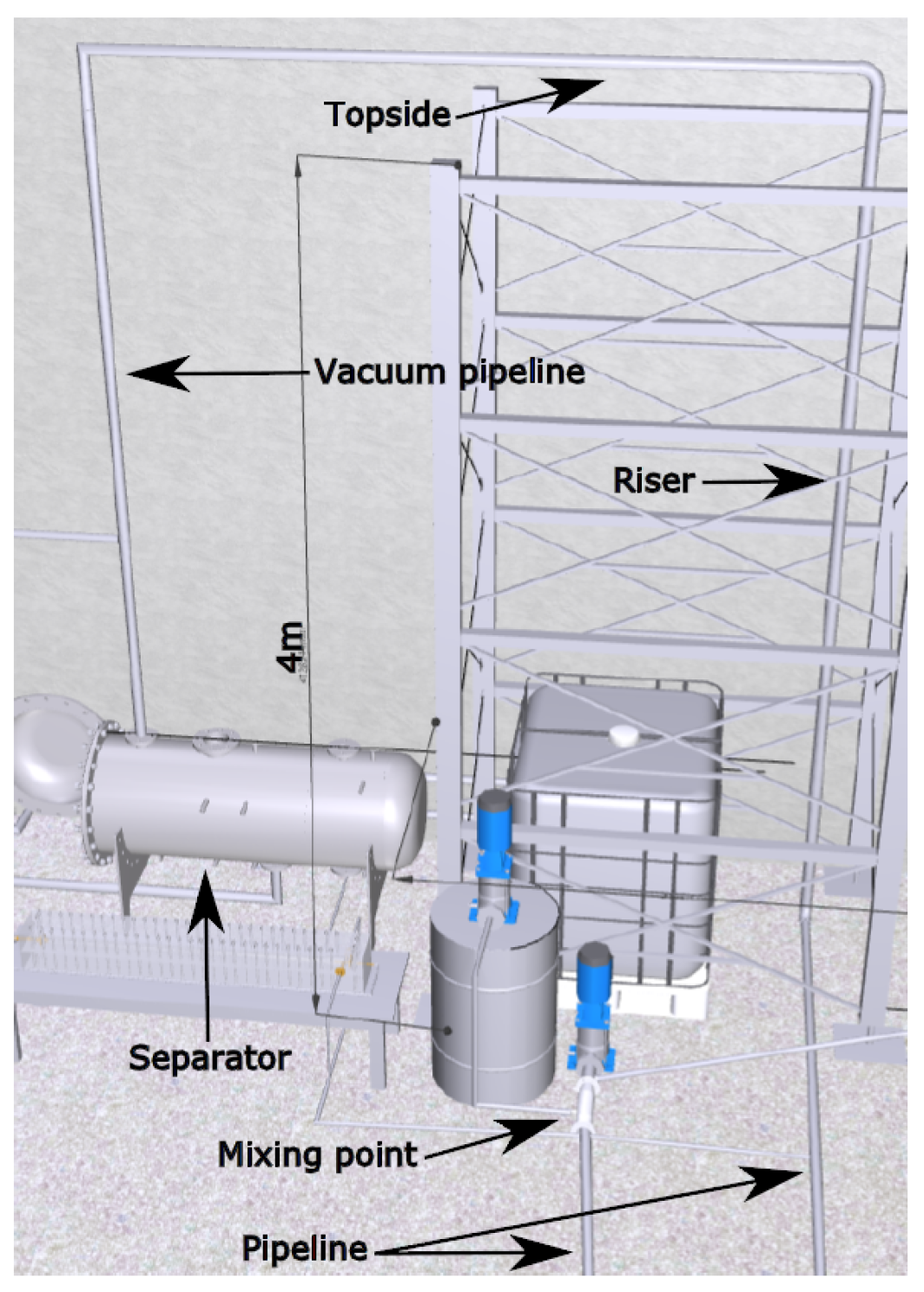
The small-scale experiments in this study is carried out on pipeline-riser slug testing facility located at Aalborg University Esbjerg. The slug testing facility is an extension of the facility examined in [11,18]. The new testing facility can be observed in Figure 1. The physical changes in the testing facility mainly consist of longer pipelines: 16 m horizontal pipeline, 4 m inclination pipeline, 4 m riser and 1.2 m topside pipeline from riser top to the topside choke valve. The outlet of the topside choke valve is connected to a vertical descending vacuum pipeline 3 m down to a 3-phase gravity separation, where the gas-liquid separation is carried out. The gravity separator is specially designed and currently has a 5 min separation buffer time (for the examined inflow conditions), however the weir level inside the separator can be adjusted in an offline manner if required for new testing conditions. The pipeline-riser dimensions can be found in

Table 1. A collection of the identified constants for the model of the testing facility.

Symbol	Description	Value	Unit
G	Gravitational constant	9.81	m/s${}^2$
R	Gas constant	8314	J/(kmol × K)
$D_p$	Pipeline diameter	$5\times {10}^{-2}$	m
$D_r$	Riser diameter	$5\times {10}^{-2}$	m
$A_c$	Pipeline cross area	$2\times {10}^{-3}$	m${}^2$
${\rho }_l$	Liquid (water) density	1000	Kg/m${}^3$
${\rho }_g$	Gas (air) density	1.649	Kg/m${}^3$
${\mu }_l$	Liquid (water) viscosity	$8.9\times {10}^{-4}$	Pa × s
${\mu }_g$	Gas (air) viscosity	$1.8\times {10}^{-5}$	Pa × s
$L_0$	Horizontal pipe length	18	m
$L_1$	Inclination pipe length	4	m
$L_2$	Riser length	4	m
$L_3$	Topside length (to valve)	1.2	m
$\theta$	Inclination pipeline angle	0.175 (${10}^{\circ }$)	Rad
$T_p$	Pipeline temperature	288.15	${}^{\circ }$K
$T_r$	Riser temperature	288.15	${}^{\circ }$K
$V_b$	Buffer (gas) tank volume	$3.9\times {10}^{-2}$	m${}^3$
$ϵ$	Pipeline roughness	$1.5\times {10}^{-6}$	m
${\gamma }_1$	Correction factor for gas	1.7	-
	flow through the lowpoint
${\gamma }_2$	Correction factor for liquid	2	-
	flow through the low point
${\gamma }_3$	Correction factor for	0.85	-
	production rate
$K_{n1}$	Tuning parameter for static	0.05	-
	valve characteristics
$K_{n2}$	Tuning parameter for static	3	-
	valve characteristics
$K_h$	Tuning parameter for steady-state	1	-
	liquid level in pipeline
$K_a$	Tuning parameter for liquid	0.78	-
	flow leaving riser during blow-out

. The pressure and flow measurement uncertainties have been reduced by installing new equipment in a narrower range than in [11,18], such that the pressure measurement uncertainty now is 0.01 bar and the flow measurement uncertainty now is $5.56\times {10}^{-4}$ kg/s. However, it has to be noted that the multi-phase flow transmitters are more uncertain the more gas is present in the pipeline, as they are measured by Coriolis flow meters. The software system is implemented in Simulink/MATLAB environment on a PC. For data acquisition an NI PCI-6229 DAQ-card is utilized and the central software system links the physical interface card through the Simulink Desktop Real-time (previously known as Real-time Windows Target) which guarantees Real-Time implementation.

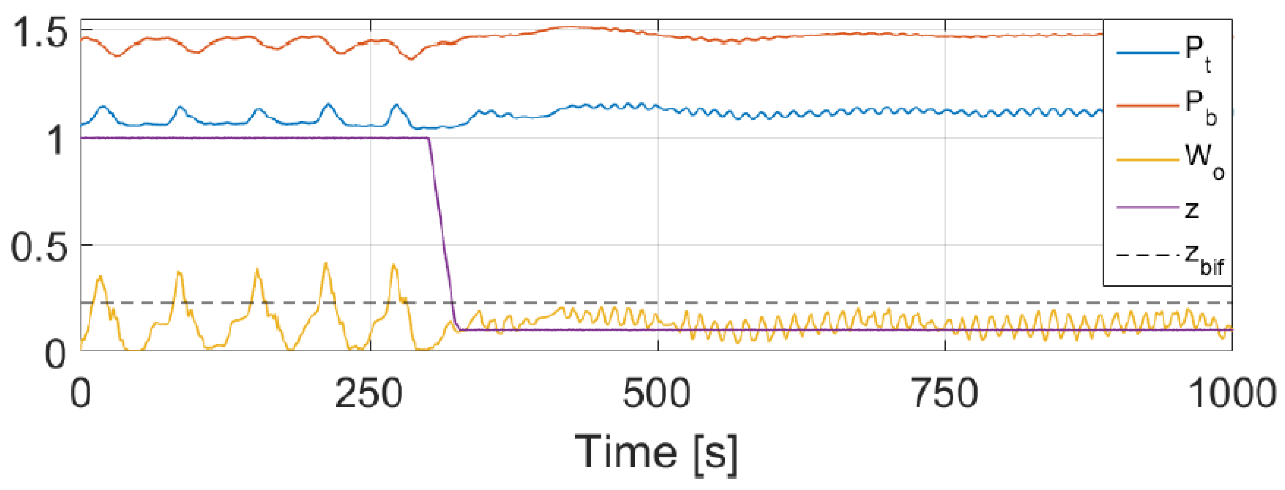
For all the tests in this paper the inflow is constant ($u_2=w_{g,in}=1.7\times {10}^{-4}$ kg/s and $u_3=w_{l,in}=1.8\times {10}^{-1}$ kg/s), with the only exceptions of the input disturbances’ tests in Section 5. The gas mass inflow is controlled by a bürkert MFC8626 solenoid valve after the compressor, and the product has a built-in PID mass flow controller for single-phase gas which has a fast tracking capability (within 5 s) without causing any visible overshooting. The liquid mass inflow is controlled by a centrifugal pump with measurement from an electromagnetic flow meter, where a PI controller is implemented, dedicated for obtaining a step response settling time under 10 s without any overshoot. The work in [19] showed that both the gas and water inflow controllers have a fast bandwidth compared to dynamics of the entire system, hence these control loops do not have any significant unintended influence to the complete system’s behavior. Figure 2 shows the step response of the slug testing facility where the valve goes from full open to 10% opening at 300 s. It is clear that the system initially is slugging before being stabilized as a consequence of the valve choking. One severe slug cycle lasts approximately 70 s. The open-loop bifurcation point (the changing from slug to steady flow) during these running conditions is at $23.4\%$ valve opening. The high frequency oscillations at non-slug flow (after 300 s) exist due to the vacuum pipeline downstream the choke valve. The pipeline is not entirely vacuum and thus sucks the flow down the pipeline in a rapid cyclic manner.

2.3. Parameter Identification

A tuning guide is carried out in [15] by isolating the dimensionless tuning parameters, $K_G$, $K_L$ and $C_v$, in the valve equations (see Equation (5)) with predefined operational points. Three correction factors were introduced: ${\gamma }_1$, ${\gamma }_2$ and ${\gamma }_3$. Each of these three new correction factors are dimensionless and should individually be close to a value of one. The relationship between the tuning parameters and the correction factors can be observed in Equations (12)–(14), where ${\rho }_{G,p}$, $\Delta P_G$, $\Delta P_L$ and ${\rho }_{rt}$ is back calculated from the steady-state measured $P_{in}$, $P_{rt}$, ${\omega }_{L,in}$, ${\omega }_{G,in}$ and $Z_1$. $Z_1$ is a non-slugging operational topside valve opening. Besides, a parameter correction factor was also considered for the steady-state level of liquid in the pipeline, $K_h$, however this correction factor performed the best for $K_h=1$.

$$\begin{array}{c}\hfill K_G=\frac{{\gamma }_1{\omega }_{G,in}}{A_G\sqrt{{\rho }_{G,p}\Delta P_G}}\end{array}$$

(12)

$$\begin{array}{c}\hfill K_L=\frac{{\gamma }_2{\omega }_{L,in}}{A_L\sqrt{{\rho }_L\Delta P_L}}\end{array}$$

(13)

$$\begin{array}{c}\hfill C_v=\frac{{\gamma }_3({\omega }_{G,in}+{\omega }_{L,in})}{Z_1{A}_c\sqrt{{\rho }_{rt}max(P_{rt}-P_s,0)}}\end{array}$$

(14)

In this study the model is further extended with a new tuning parameters, $K_a$, used to correct for how much of the liquid is flowing through the riser during the blowout stage of each slug cycle. $K_a$ can be used to adjust for offsets in the pressure. In Equation (15) $K_a$ is included to calculate the liquid-volume-fraction out of the riser (${\alpha }_{L,rt}$):

$$\begin{array}{c}\hfill {\alpha }_{L,rt}\left(t\right)=K_a(2{\alpha }_{L,r}\left(t\right)-{\alpha }_{L,rb}\left(t\right))=K_a\left(\frac{2m_{l,r}\left(t\right)}{V_r{\rho }_L}-\frac{A_{L,rb}\left(t\right)}{A_{p,rb}}\right)\end{array}$$

(15)

for ${\alpha }_{L,r}\ge {\alpha }_{L,rt}\ge 0$, where $A_{L,rb}$ is the area of liquid in riser lowpoint and $A_{p,rb}$ is the pipeline cross-section at riser lowpoint.

A collection of the identified model’s constants for the slug testing facility including the tuning parameters is listed in Table 1. The overall accuracy of the model is significantly improved with the addition of the added $K_{n1}$, $K_{n2}$ and $K_a$ tuning parameters. $K_{n1}$ and $K_{n2}$ increases the simulating accuracy for the impact of valve manipulation in the region $10\ge z\ge 90$, where the linear valve characteristic varies the most from the exponential characteristic. The inclusion of $K_a$ both improves the simulation accuracy of the riser’s hydrostatic pressure offset, as well as the pressure and flow amplitudes of the severe slugs.

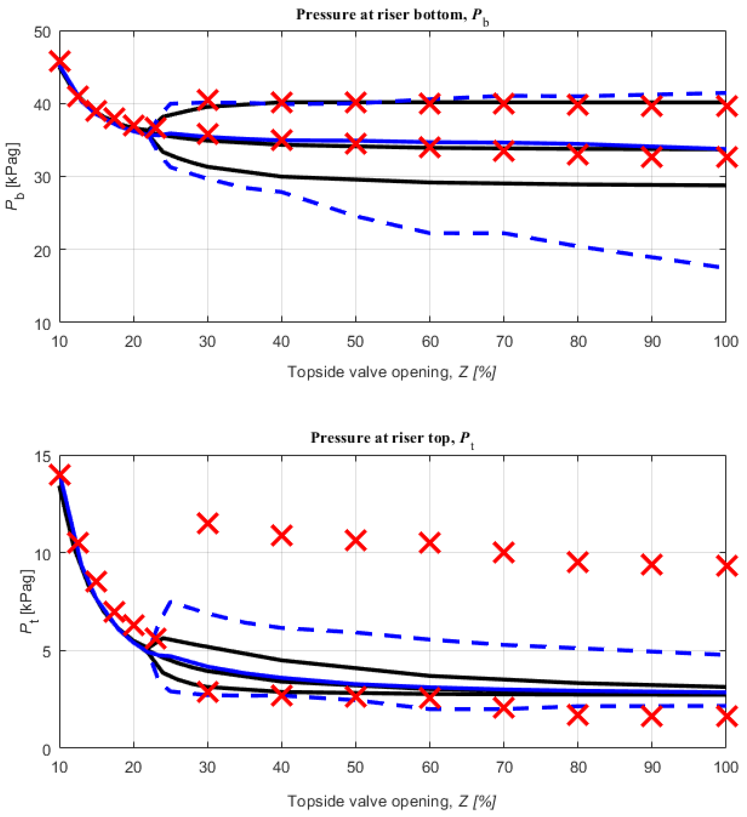
The bifurcation map of the low-dimensional (black) and OLGA model (blue) are compared with the measured pressure data (red) in Figure 3. The bifurcation map only plots the steady-state results, however it can be a useful tool to compare and validate models’ steady-state performance. It is observed that the open-loop measured bifurcation point ($Z_{bif}$) fits both models reasonably well, however, the pressures in both models vary from the measured data. At the $P_b$-plot the OLGA model seems to have a decreasing minimum peak, however this was due to high-frequency numerical peaks in the OLGA simulations and the average minimum peak was nearly constant at 28 $kPag$ for $Z\ge 40\%$. For $P_t$ is was hard to make the low-dimensional model fit the slug region with large amplitudes observed from the lab measurements. Thus it is clear that even though $Z_{bif}$ is located very close to reality for both models, the models do not fit the measurement well in the slugging region. However the fit of the bifurcation point was weighted over the amplitude peaks in the slug region for the tuning of the models, see

Table 2. The open-loop bifurcation point ($Z_{bif}$) comparison between the actual measurements from the test rig to the two models. When the models were tuned to fit the data, $Z_{bif}$ had the highest priority. Thus $Z_{bif}$ is close to reality for both models.

System	Open-Loop ${\mathit{Z}}_{\mathit{bif}}$
Test rig	23.4%
MATLAB model	23.6%
OLGA model	23.3%

. The control-oriented model will be used for the controller designs and the OLGA model will be used as a reference model for the controller implementation in Section 5.

3. System Analysis

From Figure 2 it can be observed that both top and bottom pressure measurement and the mass flow observe oscillations during a slug cycle. However at this point it is uncertain which of these measurements are preferable for control purpose. A comparison carried out in [6,13] concluded that $P_b$ is the best controlled variable for single-input-single-output (SISO) control, where $w_o$ is preferred if only considering topside measurements, while $P_t$ gave the worst results. However in [20] a pressure control comparison was made where it was concluded that $P_b$ and $P_t$ did equally well as a SISO controlled variable, where $P_t$ actually performed best. In this section two subsea pressure measurements, the pipeline inlet pressure ($P_{in}$) and the riser bottomhole pressure ($P_b$), are evaluated as well as the most applied topside measurements, riser topside pressure ($P_t$) and the topside total mass flow ($W_o$), based on Input-Output controllability (abb. controllability) analysis.

Controllability of a system is found by evaluating the minimum achievable maximal peaks of different closed-loop transfer functions [21]. The bounds are physical properties of the system and the controlled variables resulting in small peaks are preferable for a control scheme. It has to be noted that severe slugging is a highly nonlinear phenomenon and even the simple model used in this study got nonlinear properties. This is a limitation as the controllability analysis gives information of linear time-invariant systems. Hence the system analysis is based on the Jacobian linearizations of the nonlinear slug model. The peaks are found by obtaining the mean maximum value of the frequency response known as the system’s $H_{\infty }$ norm,

$$\begin{array}{c}\hfill {\left|\right|M\left|\right|}_{\infty }=\underset{0\le \omega \le \infty }{max}\left|\left|M\left(j\omega \right)\right|\right|\end{array}$$

(16)

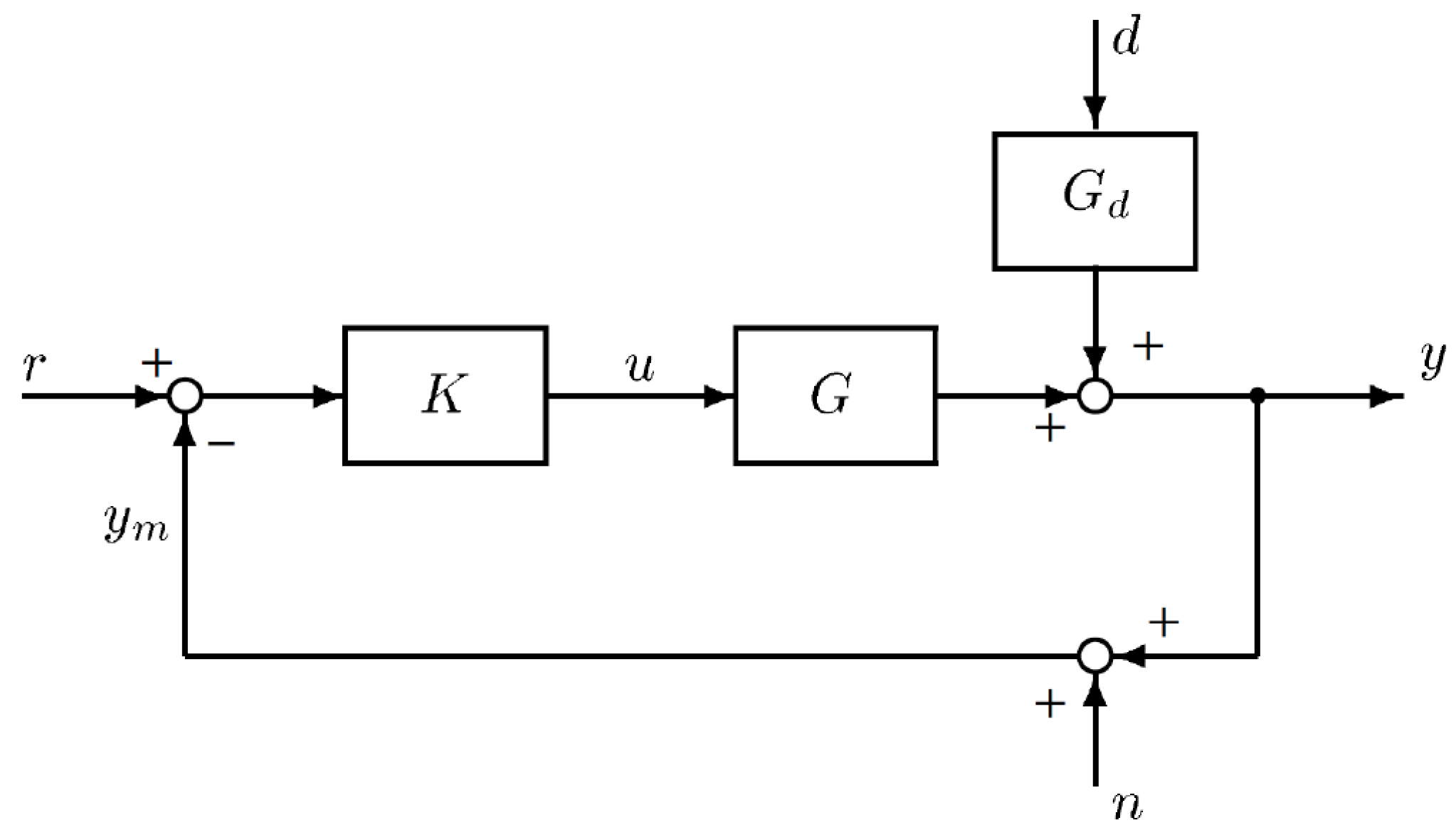
The linearized model has the form $y=G\left(s\right)u+G_d\left(s\right)d$ with a linear feedback controller $u=K\left(s\right)(r-y-n)$. Here d is the disturbances, n is the measurement noise and r is the reference setpoint. The system can be observed on Figure 4 where the system is illustrated as a block diagram. Thus, the closed-loop system is

$$\begin{array}{c}\hfill y=Tr+S{G}_{d}d-Tn,\end{array}$$

(17)

where the sensitivity transfer function is

$$\begin{array}{c}\hfill S={(I+GK)}^{-1},\end{array}$$

(18)

and the complementary sensitivity transfer function is

$$\begin{array}{c}\hfill T=GK{(I+GK)}^{-1}=I-S.\end{array}$$

(19)

The control input to the closed-loop system is

$$\begin{array}{c}\hfill u=KS(r-G_{d}d-n).\end{array}$$

(20)

$SG$ relates to the effect of the input disturbances to the control error. Besides, $KS$, $SG$ and S are considered indicators of robustness to different types of uncertainties. Normally it is prefered to keep them as small as possible to improve system robustness [13].

3.1. Lower Bounds

The equations in this section is obtained based on [21].

The lowest achievable peak values for S and T are calculated based on the distance between the unstable poles ($p_i$) and zero (z) of the open-loop system:

$$\begin{array}{c}\hfill \underset{K}{min}{\left|\right|S\left|\right|}_{\infty }\ge M_{S,min}=\prod _{i=1}^{N_p}\frac{z+p_i}{z-p_i}\end{array}$$

(21)

In [22] it was proved that Equation (21) can also be applied to the lowest peak boundary calculation of any T with no time delay, i.e., $M_{T,min}$, because the identity constraint $S+T=I$ implies that $|M_{S,min}|\ge |M_{T,min}|+1$. Furthermore, in [22] a more general boundary calculation was presented for Multiple Input Multiple Output (MIMO) systems with no time delay which also can handle multiple Right Half-Plane (RPH) zeros:

$$\begin{array}{c}\hfill M_{S,min}=M_{T,min}=\sqrt{1+{\overline{\sigma }}^2(Q_p^{-1/2}{Q}_{zp}{Q}_z^{-1/2}})\end{array}$$

(22)

where

$$\begin{array}{c}\hfill {\left[Q_z\right]}_{ij}=\frac{y_{z,i}^H{y}_{z,j}}{z_i+{\overline{z}}_j},{\left[Q_p\right]}_{ij}=\frac{y_{p,i}^H{y}_{p,j}}{{\overline{p}}_i+p_j},{\left[Q_{zp}\right]}_{ij}=\frac{y_{z,i}^H{y}_{p,j}}{z_i-p_j}.\end{array}$$

(23)

The function describing $KS$ is a transfer function from n to u, and hence considers the effect of the measurement noise and output disturbances. The lowest peak of $KS$ is estimated according to

$$\begin{array}{c}\hfill {\left|\right|KS\left|\right|}_{\infty }\ge \left|G_s{\left(p\right)}^{-1}\right|,\end{array}$$

(24)

where $G_s$ is a stable transfer function where the RHP-poles of G is mirrored into the LHP. When there are multiple and complex unstable poles the peak can be calculated as

$$\begin{array}{c}\hfill {\left|\right|KS\left|\right|}_{\infty }\ge \frac{1}{{\underline{\sigma }}_H}\left(U{\left(G\right)}^{\times }\right),\end{array}$$

(25)

where ${\underline{\sigma }}_H$ is the smallest Hankel singular value and $U{\left(G\right)}^{\times }$ is the mirrored image of the antistable part of G.

Where $SG$ relates to the input disturbances and robustness against pole uncertainty, $S{G}_d$ is related to the effect of output disturbances. For any single unstable zero, denoted as z here, the lower boundaries of the $H_{\infty }$ norms of two transfer functions for $SG$ and $S{G}_d$ can be estimated according to Equations (26) and (27):

$$\begin{array}{c}\hfill {\left|\right|SG\left|\right|}_{\infty }\ge \left|G_{ms}\left(z\right)\right|\prod _{i=1}^{N_p}\frac{z+p_i}{z-p_i}\end{array}$$

(26)

$$\begin{array}{c}\hfill \left|\right|S{G}_d{\left|\right|}_{\infty }\ge \left|G_{ms,d}\left(z\right)\right|\prod _{i=1}^{N_p}\frac{z+p_i}{z-p_i}\end{array}$$

(27)

where $G_{ms}$ and $G_{ms,d}$ are the minimum phase stable versions of G and $G_d$ as both RHP poles and zeros are mirrored into LHP.

Similarly, the lower boundary of $KS{G}_d$ can be obtained from

$$\begin{array}{c}\hfill \left|\right|KS{G}_d{\left|\right|}_{\infty }\ge \frac{1}{{\underline{\sigma }}_H}(U{(G_{d,ms}^{-1}G)}^{\times })\end{array}$$

(28)

where $U{(G_{d,ms}^{-1}G)}^{\times }$ is the mirror image of the antistable part of $G_{d,ms}^{-1}G$ [13].

The pole vector for each model is obtained for optimal output selection. A large pole vector element suggests the minimum input effort required for stabilization. Equation (29) is used to calculate the pole vector based on the C matrix from the state-space model. Here t is the right normalized eigenvector associated with the unstable RHP pole (p) such that $At=pt$. For these system models (two dominant conjugated RHP poles) the pole vector can be used as an indication of the input’s influence to the output [13].

$$\begin{array}{c}\hfill y_p=Ct\end{array}$$

(29)

3.2. Controllability Results

Table 3. Model analysis for Z = 30%.

Measurement	Equilibrium	G(0)	Pole Vector	${\left|\right|\mathit{S}\left|\right|}_{\mathbf{\infty },\mathit{min}}$	${\left|\right|\mathit{KS}\left|\right|}_{\mathbf{\infty },\mathit{min}}$	${\left|\right|\mathit{SG}\left|\right|}_{\mathbf{\infty },\mathit{min}}$	$\left|\right|{\mathit{KSG}}_{\mathit{d}1}{\left|\right|}_{\mathbf{\infty },\mathit{min}}$	$\left|\right|{\mathit{KSG}}_{\mathit{d}2}{\left|\right|}_{\mathbf{\infty },\mathit{min}}$	$\left|\right|{\mathit{SG}}_{\mathit{d}1}{\left|\right|}_{\mathbf{\infty },\mathit{min}}$	$\left|\right|{\mathit{SG}}_{\mathit{d}2}{\left|\right|}_{\mathbf{\infty },\mathit{min}}$
$P_{in}$ [bar]	0.36	−2.62	3.67	1.00	0.05	0.00	0.17	0.32	0.00	0.00
$P_b$ [bar]	0.35	−2.62	3.73	1.00	0.05	0.00	0.17	0.32	0.00	0.00
$P_t$ [bar]	0.04	−2.46	1.05	1.17	0.16	1.42	0.16	0.34	0.23	0.53
${\omega }_o$ [kg/s]	0.18	0.00	156	1.00	0.00	0.00	0.16	0.34	0.03	32.4

,

Table 4. Model analysis for Z = 45%.

Measurement	Equilibrium	G(0)	Pole Vector	${\left|\right|\mathit{S}\left|\right|}_{\mathbf{\infty },\mathit{min}}$	${\left|\right|\mathit{KS}\left|\right|}_{\mathbf{\infty },\mathit{min}}$	${\left|\right|\mathit{SG}\left|\right|}_{\mathbf{\infty },\mathit{min}}$	$\left|\right|{\mathit{KSG}}_{\mathit{d}1}{\left|\right|}_{\mathbf{\infty },\mathit{min}}$	$\left|\right|{\mathit{KSG}}_{\mathit{d}2}{\left|\right|}_{\mathbf{\infty },\mathit{min}}$	$\left|\right|{\mathit{SG}}_{\mathit{d}1}{\left|\right|}_{\mathbf{\infty },\mathit{min}}$	$\left|\right|{\mathit{SG}}_{\mathit{d}2}{\left|\right|}_{\mathbf{\infty },\mathit{min}}$
$P_{in}$ [bar]	0.36	−1.17	3.60	1.00	0.21	0.00	0.35	0.62	0.00	0.00
$P_b$ [bar]	0.34	−1.17	3.73	1.00	0.20	0.00	0.33	0.64	0.00	0.00
$P_t$ [bar]	0.03	−1.10	0.58	1.88	1.31	1.44	0.32	0.68	0.23	0.53
${\omega }_o$ [kg/s]	0.18	0.00	192	1.00	0.00	0.00	0.32	0.70	0.03	32.4

,

Table 5. Model analysis for Z = 60%.

Measurement	Equilibrium	G(0)	Pole Vector	${\left|\right|\mathit{S}\left|\right|}_{\mathbf{\infty },\mathit{min}}$	${\left|\right|\mathit{KS}\left|\right|}_{\mathbf{\infty },\mathit{min}}$	${\left|\right|\mathit{SG}\left|\right|}_{\mathbf{\infty },\mathit{min}}$	$\left|\right|{\mathit{KSG}}_{\mathit{d}1}{\left|\right|}_{\mathbf{\infty },\mathit{min}}$	$\left|\right|{\mathit{KSG}}_{\mathit{d}2}{\left|\right|}_{\mathbf{\infty },\mathit{min}}$	$\left|\right|{\mathit{SG}}_{\mathit{d}1}{\left|\right|}_{\mathbf{\infty },\mathit{min}}$	$\left|\right|{\mathit{SG}}_{\mathit{d}2}{\left|\right|}_{\mathbf{\infty },\mathit{min}}$
$P_{in}$ [bar]	0.35	−0.44	3.58	1.00	0.69	0.00	0.89	1.57	0.00	0.00
$P_b$ [bar]	0.34	−0.44	3.76	1.00	0.65	0.00	0.84	1.60	0.00	0.00
$P_t$ [bar]	0.03	−0.41	0.36	3.09	6.83	0.97	0.79	1.76	0.23	0.53
${\omega }_o$ [kg/s]	0.18	0.00	212	1.00	0.01	0.00	0.80	1.78	0.03	32.4

and

Table 6. Model analysis for Z = 75%.

Measurement	Equilibrium	G(0)	Pole Vector	${\left|\right|\mathit{S}\left|\right|}_{\mathbf{\infty },\mathit{min}}$	${\left|\right|\mathit{KS}\left|\right|}_{\mathbf{\infty },\mathit{min}}$	${\left|\right|\mathit{SG}\left|\right|}_{\mathbf{\infty },\mathit{min}}$	$\left|\right|{\mathit{KSG}}_{\mathit{d}1}{\left|\right|}_{\mathbf{\infty },\mathit{min}}$	$\left|\right|{\mathit{KSG}}_{\mathit{d}2}{\left|\right|}_{\mathbf{\infty },\mathit{min}}$	$\left|\right|{\mathit{SG}}_{\mathit{d}1}{\left|\right|}_{\mathbf{\infty },\mathit{min}}$	$\left|\right|{\mathit{SG}}_{\mathit{d}2}{\left|\right|}_{\mathbf{\infty },\mathit{min}}$
$P_{in}$ [bar]	0.35	−0.14	3.57	1.00	2.35	0.00	2.73	4.79	0.00	0.00
$P_b$ [bar]	0.34	−0.14	3.78	1.00	2.22	0.00	2.53	4.85	0.00	0.00
$P_t$ [bar]	0.03	−0.13	0.24	4.74	34.6	0.48	2.40	5.41	0.23	0.53
${\omega }_o$ [kg/s]	0.18	0.00	223	1.00	0.04	0.00	2.42	5.47	0.03	32.4

show the values for all the estimated lower controllability boundaries for linearizations at $Z=30\%$, $Z=45\%$, $Z=60\%$ and $Z=75\%$. There are two disturbances which are considered separately: $d_1$ denotes $10\%$ of the nominal value of ${\omega }_{g,in}$ and $d_2$ denotes $10\%$ of the nominal value of ${\omega }_{l,in}$. $G_{d1}$ and $G_{d2}$ is then the corresponding two linearized transfer functions between $d_1$ and $d_2$ to the considered output, respectively.

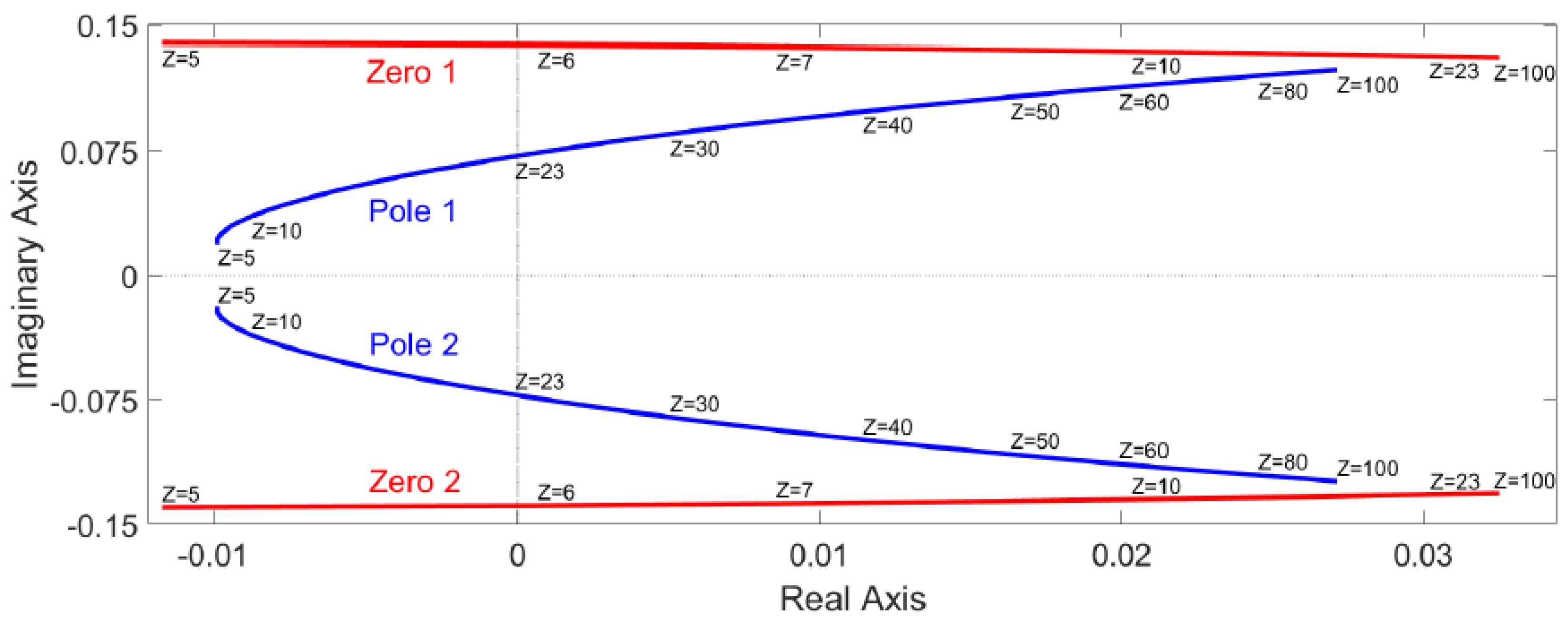
It is clear that $P_t$ in general indicates the worst possible performance, especially for the large openings ($Z>45\%$). It is also observed from ${\left|\right|S\left|\right|}_{\infty ,min}$ that only $P_t$ has RHP zeros. Figure 5 shows the pole-zero map of $P_t$ for different valve openings (linearization points). The two dominated conjugated poles get closer to two RHP zeros the higher the valve opening is, which is also observed from the Table 3, Table 4, Table 5 and Table 6. According to Equation (22) the sensitivity function rapidly increases when a RHP pole approaches a RHP zero. Furthermore ${\left|\right|KS\left|\right|}_{\infty ,min}$ and ${\left|\right|SG\left|\right|}_{\infty ,min}$ are both larger for $P_t$ which indicate the system is sensitive to measurement noise and input disturbances. For $P_b$ and $P_{in}$ the results are alike with only minor deviations from each other; both indicate acceptable properties in general and seem to handle disturbances well. Only for $Z=75\%$ the $KS$ is large and can cause problems for output noise and disturbances. $W_o$ seems to be the best solution, although it is the worst measurement for the induced disturbances in $\left|\right|KS{G}_1{\left|\right|}_{\infty ,min}$, $\left|\right|KS{G}_2{\left|\right|}_{\infty ,min}$ and especially $\left|\right|S{G}_2{\left|\right|}_{\infty ,min}$.

In general $P_t$ seems to be the worst solution for control purpose, where the three other alternatives all seem to be acceptable controlled variables. However, all four measurements seems to be able to eliminate the slug and operate beyond the open-loop bifurcation point.

4. Controller Development

The controllability analysis indicated that $P_t$ is the worst of the considered measurements to use for a control scheme. However, on many platforms $P_t$ is the only installed transmitter, as both $P_{in}$ and $P_b$ are considered too expensive due to the subsea equipment installation and maintenance, and $W_o$ can not always be directly measured as multi-phase flow transmitters still are rare due to the inaccurate measurement precision caused by the huge variations in liquid-to-gas concentrations.

For practical implementations operators often require simple anti-slug controllers, one level above the safety controllers designed by operators, e.g., minimum and maximum pressure boundaries for safe operations. The anti-slug controllers aim for (i) eliminating the severe slugs, and (ii) optimize the production rate.

The controller development is based on the linearized models as [23] concluded that a linear model with two conjugated unstable poles is sufficient for design of an anti-slug controller. Three linear control schemes are designed on the linearized models: PIDF, IMC and $H_{\infty }$ loop-shaping. All three control schemes can be applied as the K controller examined in Section 3 and are thus easy to implement. The controllers will be developed for $P_b$ and $P_t$, respectively. For both $P_b$ and $P_t$ the linearized models have 4 poles and 3 zeros, however for $P_b$ there exist two dominant conjugated poles in the RHP and one dominant zero in the LHP. For $P_t$ there two dominant conjugated poles and zeros in the RHP. In Section 5 the developed controllers will be validated based on simulations with the non-linear low-dimensional Matlab-implemented model and OLGA simulations. All the controllers included in the results can be observed in their respective transfer function form in

Table 7. Transfer functions of all the controllers developed on the low-dimensional model.

Controller Type	MV *	CV **	Transfer Function
Optimal-PIDF	z	P_b	$\frac{-15.9(s+0.083)}{s(s+1.11)}$
IMC-PIDF	z	P_b	$\frac{-19.7(s+0.137)(s+0.31)}{s(s+0.0468)}$
$H_{\infty }$ Loop-shaping	z	P_b	$\frac{-7.77(s+8.35)(s+2.17)(s^2+0.00329s+0.00579)}{s(s+0.0484)(s^2+1.22s+0.508)}$
$H_{\infty }$ Loop-shaping	z	P_b	$\frac{-2.86(s+8.35)(s+2.17)(s^2+0.00209s+0.00529)}{s(s+1.31)(s^2-0.988s+0.324)}$

* Manipulated variable. ** Controlled variable.

.

4.1. Optimal PIDF Controller Design

A Proportional–Integral–Derivative controller with low-pass filter (PIDF) controller has the following structure in the standard form:

$$\begin{array}{c}\hfill K_{PIDF}\left(s\right)=K_p(1+\frac{1}{s{T}_i}+\frac{T_{d}s}{T_{f}s+1})\end{array}$$

(30)

where $K_p$ is the proportional gain, $T_i$ is the integral time, $T_d$ is the derivative time and $T_f$ is the time constant of the derivative filter. The filter is essential for reducing the noise effect to the derivative part.

The controller was automatically tuned by using an optimization algorithm to minimize the weighted sum of a cost function ($J\left(t\right)$) for the closed-loop input and output performance, such that the optimization problem finds the minimum $J\left(t\right)$ by manipulating K using the Integrated Square Error (ISE). The cost function in Equation (32) is obtained from applying the cost from the ISE function in Equation (31) and adding an extra cost parameter:

$$\begin{array}{c}\hfill ISE={\int }_0^{\infty }{(r\left(t\right)-y\left(t\right))}^{2}dt\end{array}$$

(31)

$$\begin{array}{c}\hfill \underset{K}{min}J\left(t\right)=\underset{K}{min}{\int }_0^{\infty }\left(w_y{(r\left(t\right)-y\left(t\right))}^2+w_{u,dif}{\left|\dot{u}\left(t\right)\right|}^2\right)dt\end{array}$$

(32)

where r is the output reference, and $w_y$ and $w_{u,dif}$ are weighting values. $w_y$ is weighted the highest to prioritize the weighting of the output error the most and $w_{u,dif}$ was adjusted to take care of the physical rate limiter for the choke valves opening speed.

During the tuning it was observed that $T_i$ was problematic as an increased integral gain decreases the controllers robustness and heavily influences the oscillations of the system. However with no integral part the controller will not converge to the given setpoint. Thus a significant high $T_i$ was used for $P_b$. For $P_t$ the controller had problems handling the non-minimum phase system, generated by the RHP zero. In the OLGA simulations it was possible to manually tune a PI controller with large $T_i$ for stabilizing the system without oscillations, but with long settling time.

4.2. IMC Controller Design

Internal Model Control (IMC) includes the model in the control scheme. In this case we design the controller based on the linearized model. The IMC can also be calculated from

$$\begin{array}{c}\hfill u\left(s\right)=K(r-(y_p\left(s\right)-\tilde{y}\left(s\right)))\end{array}$$

(33)

where $y_p$ is the plant’s output and $\tilde{y}$ is the model’s output calculated as $\tilde{y}\left(s\right)=\tilde{G}\left(s\right)u\left(s\right)$ where $\tilde{G}$ is the transfer function model. The IMC structure is converted into a standard PIDF structure for K where the control parameters are tuned based on $\tilde{G}$. For more information of the structure see [24].

4.3. H-Infinity Loop-Shaping Controller Design

$H_{\infty }$ loop-shaping is based on the perturbed plant model $G_p$ to maximize the stability margin for model uncertanties. The normalized left coprime factorization of G is

$$\begin{array}{c}\hfill G=M^{-1}N.\end{array}$$

(34)

For simplification, the subscript of M and N is not included. Hence, the perturbed plant model is

$$\begin{array}{c}\hfill G_P={(M+\Delta M)}^{-1}(N+\Delta N).\end{array}$$

(35)

Here $\Delta M$ and $\Delta N$ are stable transfer functions which represent the uncertainty in the nominal plant model. The controller’s objective is to stabilize a list of perturbed plants. Hence the closed-loop feedback system is stable if and only if the nominal feedback system is stable and

$$\begin{array}{c}\hfill {\gamma }_K\stackrel{\Delta }{=}{∥\left[\begin{array}{c}K\\ I\end{array}\right]{(I-GK)}^{-1}{M}^{-1}∥}_{\infty }\le \frac{1}{ϵ}\end{array}$$

(36)

where $ϵ>0$ is the stability margin and ${\gamma }_K$ is the $H_{\infty }$ norm. When ${\gamma }_K$ is small the stability margin, $ϵ$, is correspondingly large.

5. Results and Discussion

In this section the developed controllers’ performances are investigated and compared to each other. The results are obtained using both laboratory experiments and simulations of the non-linear low-dimensional model and OLGA model, respectively. The OLGA simulations are included because it is more detailed than the low-dimensional model and thus potentially can provide more realistic results. The numerous obtained results, both from experiments and simulations, are included to give an enhanced overview of the developed controllers’ performances.

5.1. Controller Comparison

The results of the PIDF, IMC and $H_{\infty }$ loop-shaping controllers for two different independent pressure measurements ($P_t$ and $P_b$) can be observed in

Table 8. Controller comparison between $P_b$ and $P_t$ with optimal PIDF, IMC-PIDF and $H_{\infty }$ loop-shaping control schemes. The table’s result entries show the absolute maximum stable choke opening indicating the closed-loop bifurcation point for each controller respectively.

Open-Loop ${\mathit{Z}}_{\mathit{bif}}=23\%$ *	Non-Linear MATLAB Model			OLGA Model
Measurement	Optimal	IMC-PIDF	${\mathit{H}}_{\infty }$	Optimal	Tuned	IMC-PIDF	${\mathit{H}}_{\infty }$
	PIDF		Loop-Shaping	PIDF${}_{\mathit{MATLAB}}$	PIDF${}_{\mathit{OLGA}}$		Loop-Shaping
$P_b$ [bar]	62%	70%	98%	46%	59% **	47%	74%
$P_t$ [bar]	-	-	35%	-	29% **	-	41%

* The open-loop $Z_{bif}$ is 23.3 % in OLGA and 23.6 % in MATLAB. ** The controller has been retuned in OLGA to obtain better results.

. The table shows the maximum allowed choke valve openings before the closed-loop systems goes unstable ($Z_{bif}$). The results are based on simulations with the non-linear model in MATLAB and the OLGA model.

It is clear that $P_b$ gives the best performance for any of the three control schemes respectively, where $P_t$ only can stabilize with relatively low openings in both the MATLAB and OLGA simulations. The open-loop bifurcation point was not improved for $P_t$ with PIDF or IMC controllers, however by manual tuning in OLGA a PI controller was obtained which could move the bifurcation point to $29\%$ which corresponds to a relative increase of $6\%$. This solution however, had a slow converge rate as the integral gain had to be relatively low with respect to the proportional gain to guarantee stability. A similar issue was observed for $P_b$ using the PIDF control scheme, where the the integral gain had to be significantly smaller than the proportional gain to guarantee stability. Even with a low integral gain the PIDF controllers resulted in big fluctuations and long settling time for the system.

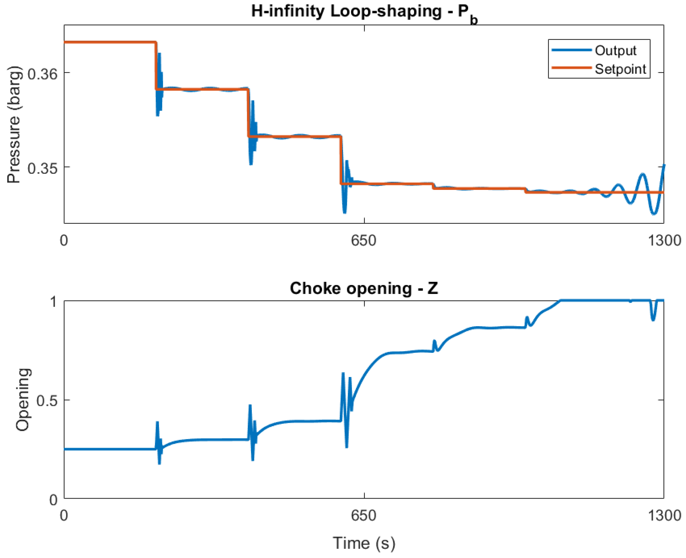
The best system performance for both $P_b$ and $P_t$ was achieved using the $H_{\infty }$ loop-shaping controller which could effectively eliminate the slug with high valve openings both in the MATLAB and OLGA simulations. The fastest settling time (≈20 s for $P_b$ at $Z=40\%$ and $\approx 65$ s for $P_t$ at $Z=40\%$) was also obtained with the $H_{\infty }$ loop-shaping controller. This is an acceptable system convergence rate with subject to the open-loop severe slug frequency ($\frac{1}{70}Hz$). Figure 6 and Figure 7 shows the MATLAB simulations of the closed-loop non-linear system performance using the $H_{\infty }$ loop-shaping controller with $P_t$ and $P_b$ respectively. It is clear that the $P_t$$H_{\infty }$ loop-shaping controller gets worse performance at high openings where it barely stabilizes the system close to the closed-loop bifurcation point, the $P_b$$H_{\infty }$ loop-shaping controller operates well at high openings, but the choke valve’s saturation cause the system to be unstable in the end.

5.2. Control with Model Disturbances

Disturbances have been introduced to the model to further evaluate the closed-loop system performances with the considered controllers.

The mass flow inputs, $w_{g,in}$ ($u_2$) and $w_{l,in}$ ($u_3$), are often only estimated on real platforms as flow transmitters not always are installed at the pipeline inlet. Thus the robustness of the controllers have been examined with input disturbance simulations in MATLAB, see

Table 9. Controller comparison between $P_b$ and $P_t$ with input and parametric disturbances based on non-linear MATLAB simulations. The result entries show the new bifurcation points for each disturbed system with the controllers from Table 8.

Non-Linear MATLAB Model Properties		${\mathit{P}}_{\mathit{b}}$			${\mathit{P}}_{\mathit{t}}$
Disturbances	Open-Loop	Optimal	IMC-PIDF	${\mathit{H}}_{\infty }$	${\mathit{H}}_{\infty }$
	${\mathit{Z}}_{\mathit{bif}}$	${\mathit{PIDF}}_{\mathit{MATLAB}}$		Loop-Shaping	Loop-Shaping
$-3\%w_{g,in}$	22%	47%	60%	98%	33%
$-6\%w_{g,in}$	21%	40%	38%	75%	-
$-3\%w_{l,in}$	24%	61%	65%	94%	32%
$-6\%w_{l,in}$	25%	60%	64%	91%	31%
$-3\%w_{g,in}$, $-3\%w_{l,in}$	23%	37%	38%	92%	32%
$-6\%w_{g,in}$, $-6\%w_{l,in}$	23%	36%	35%	87%	-
15 ${}^{\circ }$C, $W_{oil}/W_{water}=0.25$	26%	55%	68%	98%	34%
15 ${}^{\circ }$C, $W_{oil}/W_{water}=0.50$	31%	70%	70%	98%	34%
40 ${}^{\circ }$C, $W_{oil}/W_{water}=0.25$	28%	35%	72%	70%	34%
40 ${}^{\circ }$C, $W_{oil}/W_{water}=0.50$	39%	61%	82%	98%	-

. The input disturbances vary from the linearization points of the model at which the controller designs are based on. Note that the input disturbances included are negative (lower inlet mass flow), as it is experienced that systems with lower flow rates (especially for lower $w_{g,in}$) are harder for the controller to stabilize. The results show that the $H_{\infty }$ loop-shaping controller overall handles the disturbances the best. The $P_t$$H_{\infty }$ loop-shaping controller handles the disturbances well, but performs significantly worse when $w_{g,in}$ is low. For the $P_b$ the $H_{\infty }$ loop-shaping controller can still operate with large valve opening even with disturbances. The IMC-PIDF controller performed aggressively to stabilize the system, however a rate limiter was included in the simulations to emulate the valve’s opening speed. This caused the IMC-PIDF controller performance to decrease, especially for the larger steps in the setpoint. The optimal PIDF controller had an overall inadequate settling time and was considered inferior to the evaluated $P_b$ controllers.

The identified low-dimensional model is based on 2-phase flow, where the gas is air and the liquid is water. In reality the liquid phase consists of a mixture of water and crude oil, and the gas phase is methane, ethane, propane, carbon dioxide and hydrogen sulfide etc. It has to be noted that most fluids are in liquid phases in the reservoir, but phase changes can occur when the high pressure is reduced throughout the transportation pipeline. The different compositions can be considered in the model by varying the densities and viscosities. A bigger ratio of crude oil will reduce the density which correspondingly reduces the slug cycle amplitude and increases the slug cycle frequency. However the increase in crude oil also significantly increases the viscosity, which has huge impact on the friction. Table 9 include these parametric disturbances where the change in compositions are listed. For both $P_b$ and $P_t$ the controllers in general handles the disturbances well; The PIDF controller’s performance is still below the performance of the $H_{\infty }$ loop-shaping technique which is the preferred method.

The system response is acceptable for all three $P_b$ controllers, but the settling time is low for the optimal PIDF controller where no overshoot is included due to the low integral gain. The IMC-PIDF controller gives the fastest settling time in some scenarios but worst for others. The loop-shaping controller is the most robust and can operate with large valve openings, even for huge disturbances. For the $P_t$ controller the performance is very uniform over most disturbances, however for some variations the controller was not able to stabilize the system above the open-loop bifurcation point.

6. Conclusions and Future Work

This paper examines the model analysis and control design of several anti-slug controllers. The work focuses on linear controllers based on the linearized slug models but tested against the non-linear low-dimensional and OLGA models. The linearized model analysis gave an indication of which controlled variables are preferable and it was concluded that the low-point measurements are preferable over the topside transmitters where the topside flow transmitter is the best alternative if only topside measurements are available.

Slug modeling is a difficult task and it is experienced that the MATLAB and OLGA models did not fit the lab data perfectly in every aspect. The MATLAB model’s accuracy was improved by some modifications: A change in Darcy friction, an added top pressure for better estimating ${\omega }_o$, an updated static valve characteristic for $f\left(z\right)$, and a new tuning parameter for the estimating how much liquid is leaving the riser during a slug’s blowout stage. Even with these modifications, model deviations were still present, especially in the amplitude of $P_t$ during slug flow. However, this is also the case for the OLGA model. Furthermore, even though deviations from the reality exist, both the MATLAB and OLGA model are very accurate on most parameters, such as: the open-loop bifurcation point, equilibrium pressure and transient performance. Besides, the OLGA and MATLAB simulations gave consistent results. The main limitation of including the MATLAB model’s modifications, is the applicability, which to some degree compromised with more tuning parameters and extra equations.

The control solutions were based on the riser top and bottom pressures as these are the most common transmitters on offshore platforms. A comparison between optimal PIDF, IMC-PIDF and $H_{\infty }$ loop-shaping controllers were carried out based on the non-linear low-dimensional MATLAB model and on OLGA simulations. $P_b$ archieved acceptable performance with all three controllers in both the non-linear MATLAB and OLGA simulations. In MATLAB only the $H_{\infty }$ loop-shaping control technique was able to stabilize the system above the open-loop bifurcation point using the $P_t$ as the controlled variable, although $P_t$$H_{\infty }$ loop-shaping still had a relatively low $Z_{bif}$. In OLGA it was possible to find a PI controller for $P_t$ which could stabilize the system just above the open-loop bifurcation point, although the system had a long settling time due to the low integral gain required for stabilizing the system. Furthermore, the controllers was examined with input and parametric system disturbances, where the $H_{\infty }$ loop-shaping technique once again proved to be the best of the considered controller due to the controller’s ability to handle uncertain systems. For $P_t$ the controller was able to handle the disturbances in most cases but was still only able to operate with relatively low valve openings.

It is concluded the $P_b$ is the preferable pressure transmitter to use for feedback control in an anti-slug control scheme. However, if only the topside pressure transmitter is available this can still be used for eliminating the slug outside the open-loop slug region. The $H_{\infty }$ loop-shaping control solution gave the best performance for both $P_b$ and $P_t$. For a slug model a robust controller (such as $H_{\infty }$ loop-shaping) seems to handle the uncertain running conditions much better than an optimal controller (such as optimal PIDF), and furthermore the robustness does not sacrifice much of the control performance. The biggest limitation using the $H_{\infty }$ loop-shaping controllers are the significant overshoots at the output transient response before output stabilization. In future work further evaluation of the controllers’ performance will be based on implementations on the lab-scaled testing rig. This has not been possible as the testing facility has been further modified after the system identification data was obtained, and thus the model has to be updated and re-identified with the new facility dimensions.

References

- Pedersen, S.; Durdevic, P.; Yang, Z. Challenges in slug modeling and control for offshore oil and gas productions: A review study. Int. J. Multiph. Flow 2017, 88, 270–284. [Google Scholar] [CrossRef]
- Hill, T.J.; Wood, D.G. Slug flow: Occurrence, consequences, and prediction. In Proceedings of the University of Tulsa Centennial Petroleum Engineering Symposium, Tulsa, Oklahoma, 29–31 August 1994. [Google Scholar]
- Havre, K.; Stornes, K.O.; Stray, H. Taming slug flow in pipelines. ABB Rev. 2000, 4, 55–63. [Google Scholar]
- Havre, K.; Dalsmo, M. Active Feedback Control as the Solution to Severe Slugging. In Proceedings of the SPE Annual Technical Conference & Exhibition, San Antonio, TX, USA, 9–11 October 2017. [Google Scholar]
- Ogazi, A.I. Multiphase Severe Slug Flow Control. Ph.D. Thesis, School of Engineering, Department of Offshore, Process and Energy Engineering, Cranfield University, Cranfield, UK, 2011. [Google Scholar]
- Jahanshahi, E. Control Solutions for Multiphase Flow—Linear and Nonlinear Approaches to Anti-Slug Control. Ph.D. Thesis, Norwegian University of Science and Technology, Trondheim, Norway, 2013. [Google Scholar]
- Hu, B. Characterizing Gas-Lift Instabilities. Ph.D. Thesis, Norwegian University of Science and Technology (NTNU), Trondheim, Norway, 2004. [Google Scholar]
- Jepsen, K.; Hansen, L.; Mai, C.; Yang, Z. Emulation and Control of Slugging Flows in a Gas-Lifted Offshore Oil Production Well Through a Lab-sized Facility. In Proceedings of the IEEE International Conference on Control Applications (CCA), Hyderabad, India, 28–30 August 2013; pp. 906–911. [Google Scholar]
- Jansen, F.E.; Shoham, O.; Taitel, Y. The Elimination of severe slugging - experiments and modeling. Int. J. Multiph. Flow 1996, 22, 1055–1072. [Google Scholar] [CrossRef]
- Ogazi, A.; Cao, Y.; Yeung, H.; Lao, L. Slug Control With Large Valve Openings To Maximize Oil Production. SPE J. 2010, 15, 3. [Google Scholar] [CrossRef]
- Pedersen, S.; Durdevic, P.; Yang, Z. Learning control for riser-slug elimination and production-rate optimization for an offshore oil and gas production process. In Proceedings of the 19th World Congress of the International Federation of Automatic Control, Cape Town, South Africa, 24–29 August 2014; pp. 8522–8527. [Google Scholar]
- De Oliveira, V.; Jäschka, J.; Skogestad, S. An Autonomous Approach for Driving Systems towards Their Limit: An Intelligent Adaptive Anti-Slug Control System for Production Maximization. In Proceedings of the 2nd IFAC Workshop on Automatic Control in Offshore Oil and Gas Production, Florianopolis, Brazil, 27–29 May 2015; pp. 104–111. [Google Scholar]
- Jahanshahi, E.; Skogestad, S.; Helgesen, A.H. Controllability analysis of severe slugging in well-pipeline-riser systems. In Proceedings of the IFAC Workshop on Automatic Control in Offshore Oil and Gas Production, NTNU, Trondheim, Norway, 31 May–1 June 2012; pp. 101–108. [Google Scholar]
- Jahanshahi, E.; Oliveira, V.D.; Grimholt, C.; Skogestad, S. A comparison between Internal Model Control, optimal PIDF and robust controllers for unstable flow in risers. In Proceedings of the 19th World Congress, The International Federation of Automatic Control (IFAC’14), Cape Town, South Africa, 24–29 August 2014; pp. 5752–5759. [Google Scholar]
- Jahanshahi, E.; Skogestad, S. Simplified Dynamic Models for Control of Riser Slugging in Offshore Oil Production; SPE 172998; Society of Petroleum Engineers: Richardson, TX, USA, 2014; pp. 40–55. [Google Scholar]
- Drew, T.B.; Koo, E.C.; McAdams, W.H. The Friction Factor for Clean Round Pipes. Trans. AIChe 1932, 28, 56–72. [Google Scholar]
- Haaland, S.E. Simple and Explicit Formulas for the Friction Factor in Turbulent Flow. J. Fluids Eng. (ASME) 1983, 105, 89–90. [Google Scholar] [CrossRef]
- Biltoft, J.; Hansen, L.; Pedersen, S.; Yang, Z. Recreating Riser Slugging Flow Based on an Economic Lab-sized Setup. In Proceedings of the 5th IFAC International Workshop on Periodic Control Systems, Caen, France, 3–5 July 2013; pp. 47–52. [Google Scholar]
- Pedersen, S. Plant-Wide Anti-Slug Control for Offshore Oil and Gas Processes. Ph.D. Thesis, Aalborg University, Aalborg, Denmark, 2016. [Google Scholar]
- Meglio, F.D.; Petit, N.; Alstadb, V.; Kaasab, G.O. Stabilization of slugging in oil production facilities with or without upstream pressure sensors. J. Process Control 2012, 22, 809–822. [Google Scholar] [CrossRef]
- Skogestad, S.; Postlethwaite, I. Multivariable Feedback Control: Analysis and Design; Wiley & Sons: Hoboken, NJ, USA, 2005. [Google Scholar]
- Chen, J. Logarithmic integrals, interpolation bounds and performance limitations in MIMO feedback systems. IEEE Trans. Autom. Control 2000, 45, 1098–1115. [Google Scholar] [CrossRef]
- Jahanshahi, E.; Skogestad, S. Closed-loop model identification and PID/PI tuning for robust antislug control. In Proceedings of the 10th IFAC International Symposium on Dynamics and Control of Process Systems, Mumbai, India, 18–20 December 2013; pp. 233–240. [Google Scholar]
- Jahanshahi, E.; Skogestad, S. Anti-slug control solutions based on identified model. J. Process Control 2015, 30, 58–68. [Google Scholar] [CrossRef]
Figure 1.
An illustrative 3D drawing of the test rig at Aalborg University Esbjerg. The figure shows the mixing point between liquid and gas to a horizontal pipeline joint with a riser and a vacuum pipeline down to a 3-phase separator at ground level. The illustration does not include the choke valves since they can be moved along all pipeline and riser sections.
Figure 2.
A choke valve (z) step test from 100% (slug flow) to 10% (non-slug flow) opening at 300 s. The open-loop bifurcation point is located at illustrated by the black dashed line. The riser top pressure () in bar is the blue characteristic, The riser bottom pressure () in bar is the red characteristic, and the mass flow out of the system () measured by a Coriolis mass flow transmitter in kg/s is the yellow characteristic.
Figure 3.
The and bifurcation maps of the low-dimensional model (blue), OLGA model (black) and data from slug testing facility (red).
Figure 4.
Block diagram showing the considered system including output disturbance (d) and measurement noise (n).
Figure 5.
The pole-zero map of z to ’s transfer function with linearizations from 5 to 100% valve openings. The model consists of 4 poles and 3 zeros. It is clear that two dominated conjugated poles (blue) approach the two Right Half-Plane (RHP) zeros (red) at high valve openings. The last 2 poles and zero are located far out on Left Half-Plane (LHP) real axis (not plotted) and are thus insignificant to the system performance.
Figure 6.
The non-linear model with the loop-shaping controller for . The setpoint is stepped to find highest allowed valve opening. At 1000 s the system stabilizes at highest allowed opening before reaching the closed-loop bifurcation point.
Figure 7.
The non-linear model with the loop-shaping controller for . The setpoint is stepped to find highest allowed valve opening. At 1000 s the system cannot stabilize due to the saturation of the choke valve.