Acceleration of Gas Flow Simulations in Dual-Continuum Porous Media Based on the Mass-Conservation POD Method

1
National Engineering Laboratory for Pipeline Safety, China University of Petroleum, Beijing 102249, China
2
MOE Key Laboratory of Petroleum Engineering, China University of Petroleum, Beijing 102249, China
3
Beijing Key Laboratory of Urban Oil and Gas Distribution Technology, China University of Petroleum, Beijing 102249, China
4
Key Laboratory of Thermo-Fluid Science and Engineering, Xi’an Jiaotong University, Ministry of Education, Xi’an 710049, China
5
Computational Transport Phenomena Laboratory, Division of Physical Science and Engineering, King Abdullah University of Science and Technology, Thuwal 23955-6900, Saudi Arabia
6
School of Mechanical Engineering, Beijing Institute of Petrochemical Technology, Beijing 102617, China
*
Author to whom correspondence should be addressed.
Energies 2017, 10(9), 1380; https://0-doi-org.brum.beds.ac.uk/10.3390/en10091380
Submission received: 17 August 2017
/
Revised: 6 September 2017
/
Accepted: 7 September 2017
/
Published: 12 September 2017
(This article belongs to the Special Issue Flow and Transport Properties of Unconventional Reservoirs)
Abstract
:Reduced-order modeling approaches for gas flow in dual-porosity dual-permeability porous media are studied based on the proper orthogonal decomposition (POD) method combined with Galerkin projection. The typical modeling approach for non-porous-medium liquid flow problems is not appropriate for this compressible gas flow in a dual-continuum porous media. The reason is that non-zero mass transfer for the dual-continuum system can be generated artificially via the typical POD projection, violating the mass-conservation nature and causing the failure of the POD modeling. A new POD modeling approach is proposed considering the mass conservation of the whole matrix fracture system. Computation can be accelerated as much as 720 times with high precision (reconstruction errors as slow as 7.69 × 10⁻⁴%~3.87% for the matrix and 8.27 × 10⁻⁴%~2.84% for the fracture).
1. Introduction
A dual-porosity, dual-permeability (dual-continuum) model is an important conceptual model for unconventional oil/gas flow in fractured reservoirs [1,2,3,4]. Its computational consumption is very large for solving the two coupled sets of partially differential equations for fluid flows in the matrix and the fracture [5,6], which is not endurable in engineering for analyzing the long-term transient characteristics of flow in fractured porous media. Due to the high computational cost, many analytical solutions have been proposed [7,8,9,10,11]. However, analytical solutions can only be obtained under much idealized assumptions, such as slight compressibility, infinite radial flow, homogenization etc., so that their applications are very limited to simplified cases of oil flow. For gas flow, the slight compressibility assumption is no longer held, leading to nonlinear equations which cannot be analytically solved. Therefore, gas flow simulation in dual-continuum porous media has the same computational problem as has also existed with other problems [12] and has its own problems such as strong nonlinearity. It is urgent to develop an efficient numerical method for gas flow in dual-porosity, dual-permeability porous media.
Proper orthogonal decomposition (POD) is an efficient numerical method to largely accelerate the computational speed via project governing equations onto low dimensional eigen spaces to establish a reduced-order model. It has been widely utilized for many non-porous-medium flow problems [13,14,15] and also proved to be efficient for some liquid flow cases in single-continuum porous media [16,17]. In reference [16], Ghommem et al. discussed a high-precision mode decomposition method for a time-dependent incompressible single-phase flow, but did not describe the acceleration performance of the method. In reference [17], a POD Galerkin model is proposed for an incompressible single-phase flow. Only four samples and two modes used in the model can predict hundreds of cases with high-precision and fast-computation. This research is all on incompressible single-phase flow. The flow domain is a single-continuum porous media. To the best knowledge of the authors, no work has been reported for a POD model of compressible single-phase gas flow in dual-continuum porous media, which has much higher computational cost than single-continuum porous media. Thus, POD has larger potential to accelerate the numerical computation of gas flow in dual-continuum porous media. In this study, we proposed a POD acceleration method for gas flow in fractured porous media based on a dual-porosity, dual-permeability model for the first time. The principle for the POD modeling of this complex flow system is discussed to guide the improvement of the POD modeling of a dual-continuum, porous-medium compressible flow system. The precision and acceleration of the improved POD model are examined.
2. Problems Arising from the Typical POD Modeling Approach
2.1. Model Derivation via the Typical Approach
For statement convenience, we only consider ideal gas flow in two-dimensional Cartesian coordinates in this paper. Darcy’s law is as follows:
Governed by the Darcy’s law, mass conservation equations for gas flow in dual-porosity dual-permeability porous media become:
where , , , , are porosity, pressure, injection/production rate and two components of conductivity (diagonal permeability tensor divided by dynamic viscosity ). The subscripts M and F represent the matrix and fracture respectively. is the intrinsic conductivity of the matrix for the matrix–fracture interaction term. T is temperature. is the molecular weight of gas. R is the universal gas constant (8.3147295 J/(mol·K)). is the shape factor of the fracture, taking the form proposed by Kazemi [18]:
where and are the lengths of the fracture spacing in the x and y directions respectively. The last terms of Equations (3) and (4) are interaction terms between matrix and fracture.
To establish the POD model for this flow system, pressure is assumed to be the following linear combination:
where consists of and with corresponding spatial modes for matrix pressure () and fracture pressure (), respectively, so that and , are the temporal coefficients, and N is the number of POD modes. Substitute Equation (6) to Equations (3) and (4) to obtain the variable-separated Equations (7) and (8):
According to the typical procedure of POD modeling, one should project the matrix equation, Equation (7), onto and project the fracture equation, Equation (8), onto , respectively (m = 1~N), and add these two projection equations together to solve the unique temporal coefficients (n = 1~N). The procedure will be explained as follows. First of all, the projections of Equations (7) and (8) are expressed as:
where lx and ly are the domain length in the x and y directions, respectively. Note that is only the spatial function and is only the temporal function. Using this property, the above two equations can be transformed to:
The first integrations on the right hand side of Equations (11) and (12) can be transformed using integration by part:
By substituting these two expressions back to the first term of right hand side of Equations (11) and (12), one can obtain the following expressions:
For the Dirichlet boundary condition, the boundary pressure gradients in Equations (15) and (16) can be expressed as:
where i and j are the index of the grid points in the x and y directions, respectively; nx and ny are grid numbers; and and are corresponding grid spaces. K = M for the matrix and F for the fracture.
For the Neumann boundary condition, boundary pressure gradients can be expressed via Darcy’s law (Equations (1) and (2)). Substitute Equations (15) and (16) and the boundary conditions to Equations (11) and (12), and the projection equations can be expressed as follows:
Projection equation of the matrix:
Projection equation of the fracture:
where , ,
- ,
- ,
- ,
- ,
- , .
k = M for the matrix and F for the fracture. Diri is 1 for the Dirichlet boundary and 0 for the Neumann boundary. To uniquely solve the value of the POD coefficients, Equations (18) and (19) should be added to obtain the final POD projection equation of the dual-porosity, dual-permeability system:
where , , , , , , .
2.2. Numerical Methods and Parameters
Equation (20) is the POD model for the gas flow in dual-porosity, dual-permeability porous media using the typical modeling approach. The temporal advancement of coefficients can be expressed by the following linear algebraic equations:
where , . Starting with initial coefficients , the coefficients for every time step can be calculated via Equation (21). comes from the inner product of initial pressure onto POD modes:
The symbol “·” means inner product. Equation (22) exists because of an important property of POD modes, namely that they are unitary vectors orthogonal to each other, i.e., . To calculate the temporal coefficients of the POD model in Equation (21), and should be firstly calculated by POD modes. The modes are generated from the following sampling and eigenvalue decomposition process:
- (1)
- Through the numerical computation of Equations (3) and (4), a sample matrix of pressure can be collected at different moments as:where Ns is the number of samples. To ensure stability and accuracy at a large time step, we used the semi-implicit finite difference method (FDM) to compute Equations (3) and (4). With the samples, a kernel for the eigenvalue decomposition can be calculated as follows:
- (2)
- Take the eigenvalue decomposition for the kernel to obtain eigenvalues and eigenvectors:where are the eigenvalues; and is the corresponding eigenvector matrix.
- (3)
- Calculate the POD modes using the eigenvectors and samples:where “” means L2 norm.
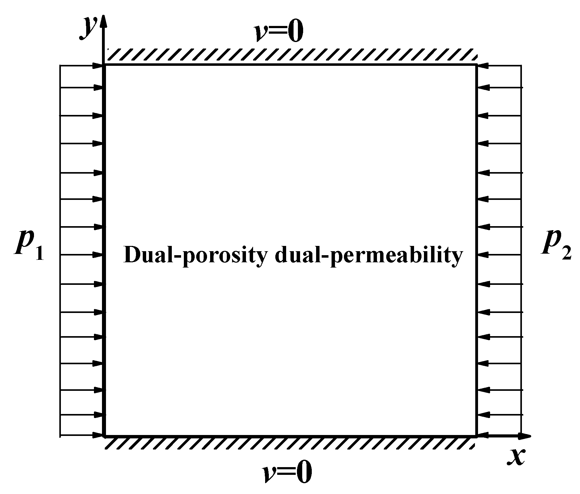
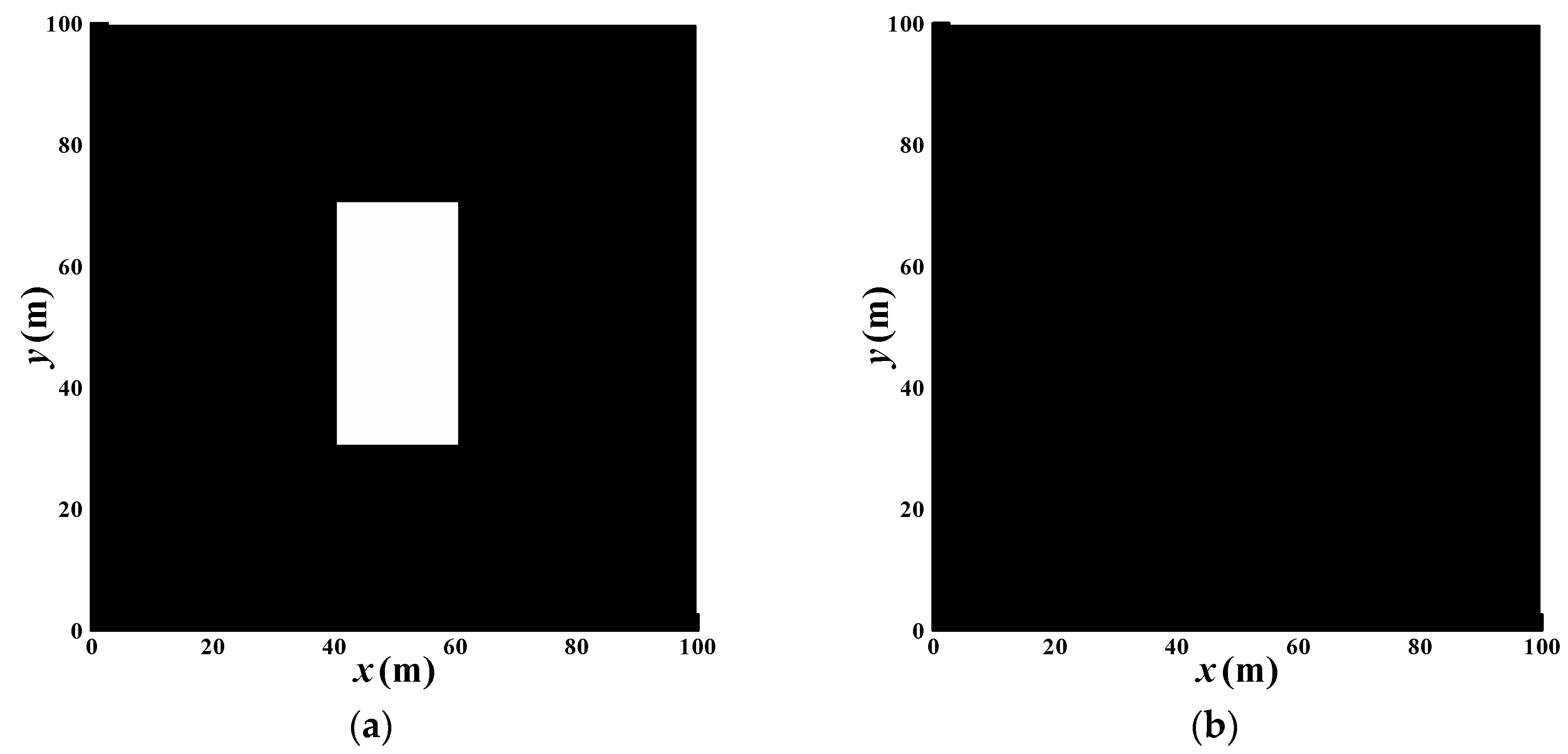
A numerical case is designed for the gas flow in the dual-porosity, dual-permeability porous media. The computational domain and boundary conditions are shown in Figure 1. Permeability is assumed to be isotropic with spatial distribution (Figure 2). The gas property was chosen to be methane as it is the main composition of natural gas. Uniform mesh was used. Sampling was made every 10 time steps. Other parameters are listed in Table 1.
2.3. Problem Analyses
The typical POD model for gas flow in dual-porosity, dual-permeability porous media (Equations (6) and (21)) is computed using the above parameters. To examine the deviation quantitatively, the relative error for pressures in the matrix and the fracture are defined as follows:
where and are matrix pressure and fracture pressure computed by FDM in Equations (3) and (4), and are corresponding pressures computed by the POD model. The details of the FDM algorithm are as follows. The temporal advancement for the whole equation system is a semi-implicit method. The diffusion terms in Equations (3) and (4) are discretized using the second-order cell-centered finite difference scheme. A staggered grid, where velocity components are placed on the cell surfaces of the pressure grid, is used to ensure the computational stability. The discrete equations via these FDM algorithms can be easily solved using the linear solver of algebraic equations.
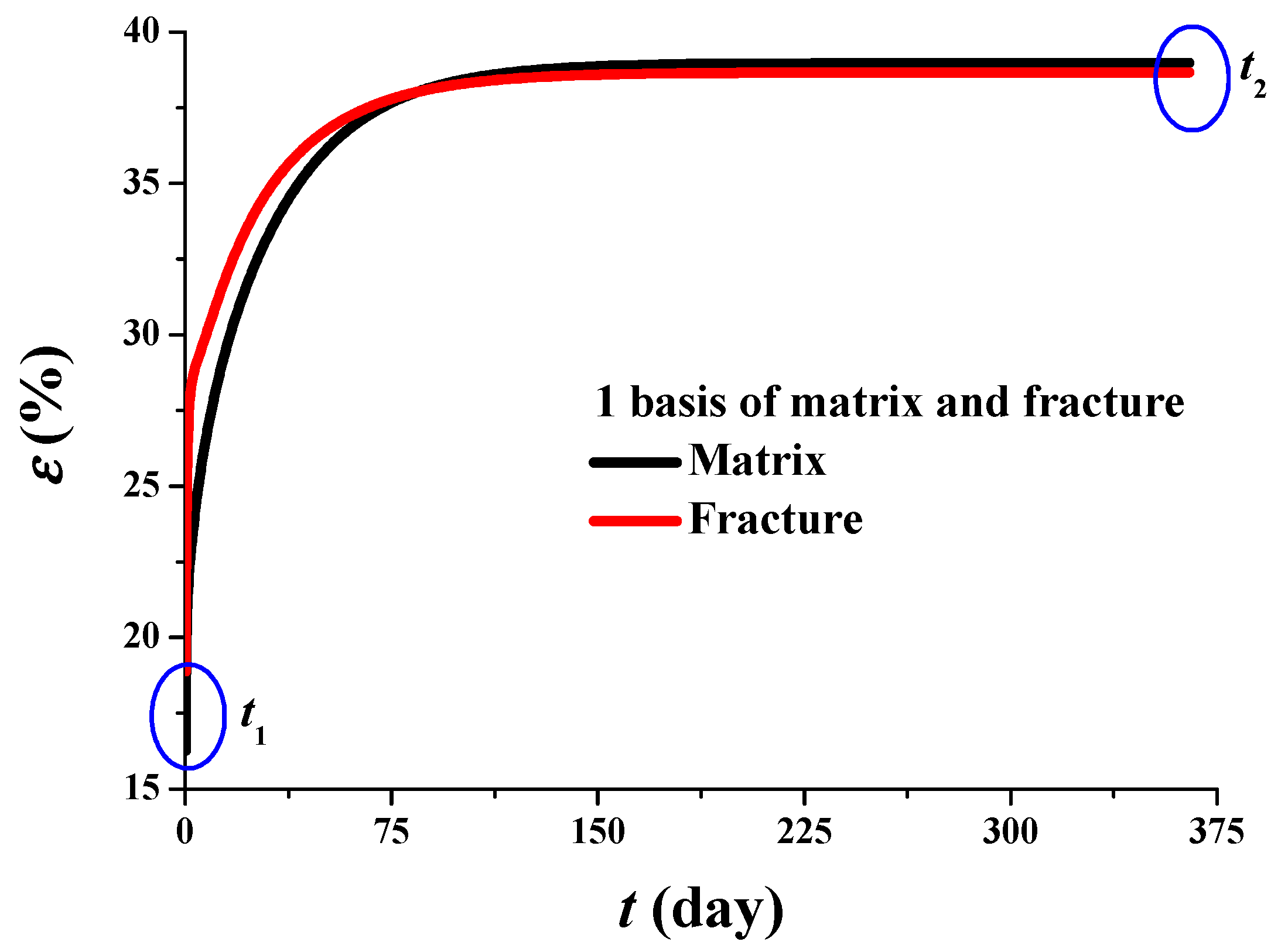
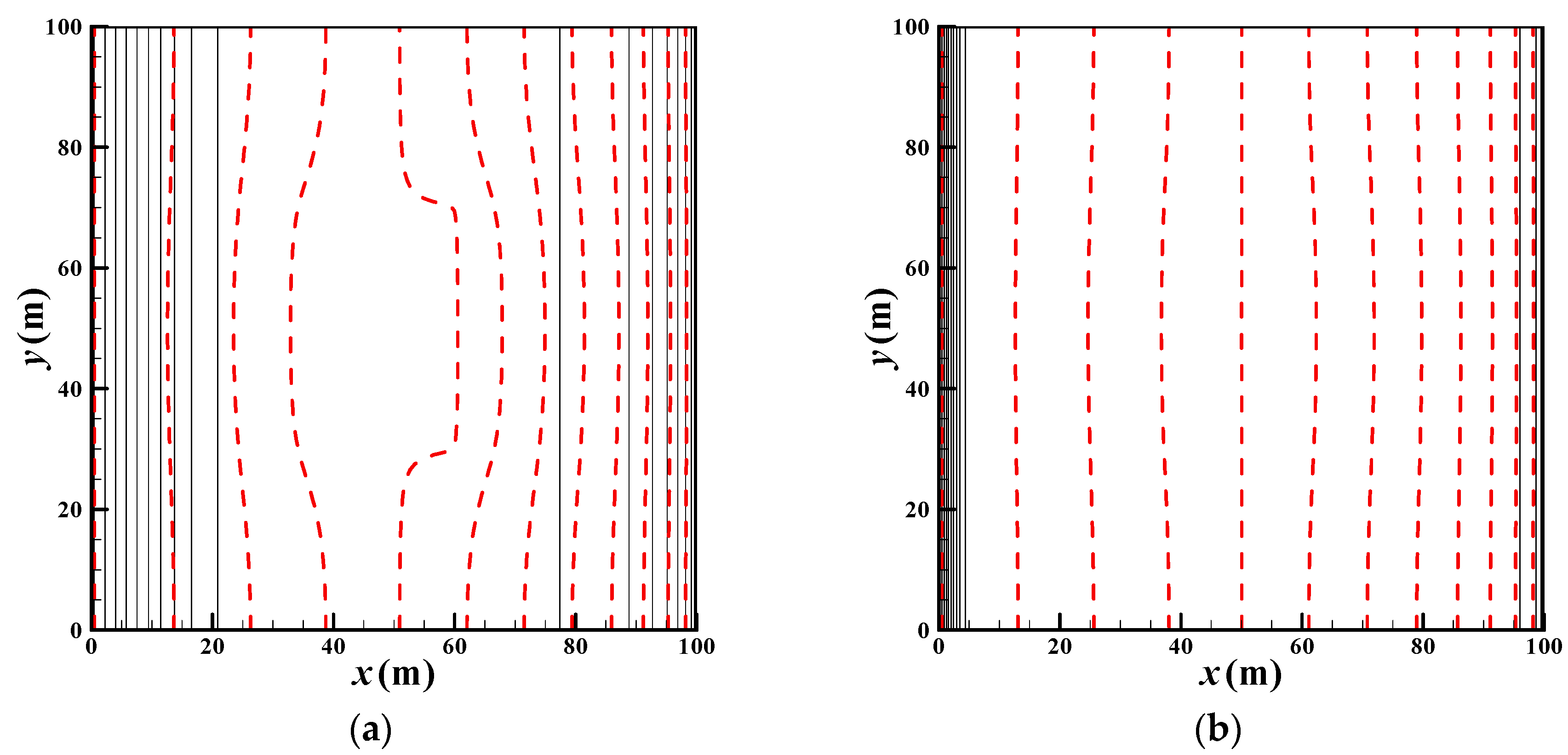
It is unusual that the typical POD model can only be computed when the top one POD modes of matrix and fracture ( and ) are used. If more POD modes are used in the POD model, the computation will be broke up. For the POD results using the top one POD modes, the relative errors are very large all over the whole transient process (18.89~38.67% for the fracture pressure and 16.26~38.98% for the matrix pressure), as shown in Figure 3. It is further confirmed in Figure 4 and Figure 5 that the reconstructed pressure fields for both the fracture and matrix cannot reproduce pressure fields accurately at the two moments: t1 and t2. Thus, the typical POD model has quite low robustness and low precision, and it should be improved.
Before the improvement of the above POD model, the reason for the low robustness and low precision should be revealed firstly to clarify the direction of improvement. We revisited the governing equations (Equations (3) and (4)) of the gas flow in dual-porosity, dual-permeability porous media and realized that these two equations actually reflect the mass transfer of gas between the matrix and fracture. The term in Equation (3) represents the mass leaving the matrix. The term in Equation (4) represents the mass entering the fracture. The mass of gas in the matrix and fracture changes every second, but the total mass for the whole system does not change. Mass is only transferred from the matrix part to the fracture part so that the net mass transfer should be zero. Therefore, the projection of the net mass transfer should also be zero. However, in the typical POD modeling approach, the transfer term in Equation (3) is projected onto while the transfer term in Equation (4) is projected onto so that the projection of the net mass transfer could not be zero. This non-zero term is generated from the projection process but not from its physical nature. Thus, the typical POD modeling is correct in mathematics but incorrect in physics because it induces artificial mass transfer of the whole system, which does not exist in nature.
To verify the above theoretical analyses, we examine the value of and compare its magnitude with other terms. It is obvious that according to the definition of integration. Therefore, in Equation (20) can represent the projection of the net mass transfer . For convenience of comparison, we define a ratio of the net mass transfer to the diffusion term:
The ratio is −3.62 × 10², −1.98 × 10³ and 4.85 × 10³ for N = 1, 2, 3 respectively in Table 2. This means that the effect of the matrix–fracture interaction is hundreds or thousands of times larger than the effect of the diffusion, so that the behavior is indeed controlled by the matrix–fracture interaction in the typical POD modeling. However, this interaction effect is artificially generated from the projection of the transfer term and separately in the matrix equation and fracture equation. Thus, the large unphysical mass transfer term causes the computation of the typical POD model to have very low precision (N = 1) or even to be broken up (N > 1). It is confirmed by the above comparison that the previous theoretical analyses are correct quantitatively. To obtain a reliable and accurate POD model for the dual-porosity, dual-permeability system, the artificial mass transfer should be avoided.
3. A New POD Modeling Approach Based on System Mass Conservation
3.1. Establishment of the New POD Model
According to the theoretical analysis and numerical comparison in Section 2.3, we realized that the separate projections of the interaction terms in matrix Equation (3) and fracture Equation (4) in the typical POD modeling approach introduces artificial mass transfer between matrix and fracture which does not exist in nature. Although it is correct in mathematics, the typical approach violates the mass conservation of the whole dual-continuum system in physics. A new POD modeling approach should be developed obeying both mathematics and physics.
From the analyses in Section 2.3, we recall that the mass is only exchanged between the matrix part and the fracture part, but the net mass transfer for the whole system is zero. This kind of mass conservation is automatically ensured in FDM but not automatically ensured in the typical POD modeling approach. To guarantee the mass conservation in the POD modeling, we propose a new approach in which the summation of Equations (3) and (4) is made before their projection. After the summation, the mass conservation equation of the whole system is:
This equation can be projected onto either or . Using a general symbol (* = M or F representing the matrix or fracture respectively) in a similar projection process to that in Section 2.1, the projection equation of Equation (30) can be expressed as follow:
where , ,
- ,
- ,
- ,
- ,
Equation (31) does not contain the projection of interaction terms, such as in Equation (20), so that no artificial mass transfer exists. Thus, it represents the mass conservation of the whole system in physical nature. The derivation also obeys mathematical laws strictly.
3.2. Model Verification
A new POD model based on the mass conservation of the whole system is established in Section 3.1 theoretically. Its precision and computational speed should be verified by the same numerical case in Section 2.2. First of all, the projection operator or needs to be discussed to determine the exact model expression. For convenience of comparison, the relative errors in Equations (27) and (28) are averaged in time. The time-averaged errors of the matrix pressure and the fracture pressure are listed in Table 3 and Table 4. The time-averaged errors have slight differences between the projections onto and when the numbers of the POD modes are from 1 to 4. However, the POD model based on the projection of cannot obtain results for due to the break-up of the computation. This is because the gas in the matrix flows much more slowly than the gas in the fracture, i.e., changes much faster than in the same time scope. Thus, the values of in samples are in a very small range, leading the base to contain more numerical errors than (the numerical errors are generated from the POD decomposition). Thus, the blow up using more modes () indicates that only the first four modes of the base contain information on fracture pressure while the following modes () are all numerical errors with no physical meaning. Thus, the new POD modeling approach can only use the projection of matrix mode, i.e., the superscript “*” in Equation (31), and is “M”.
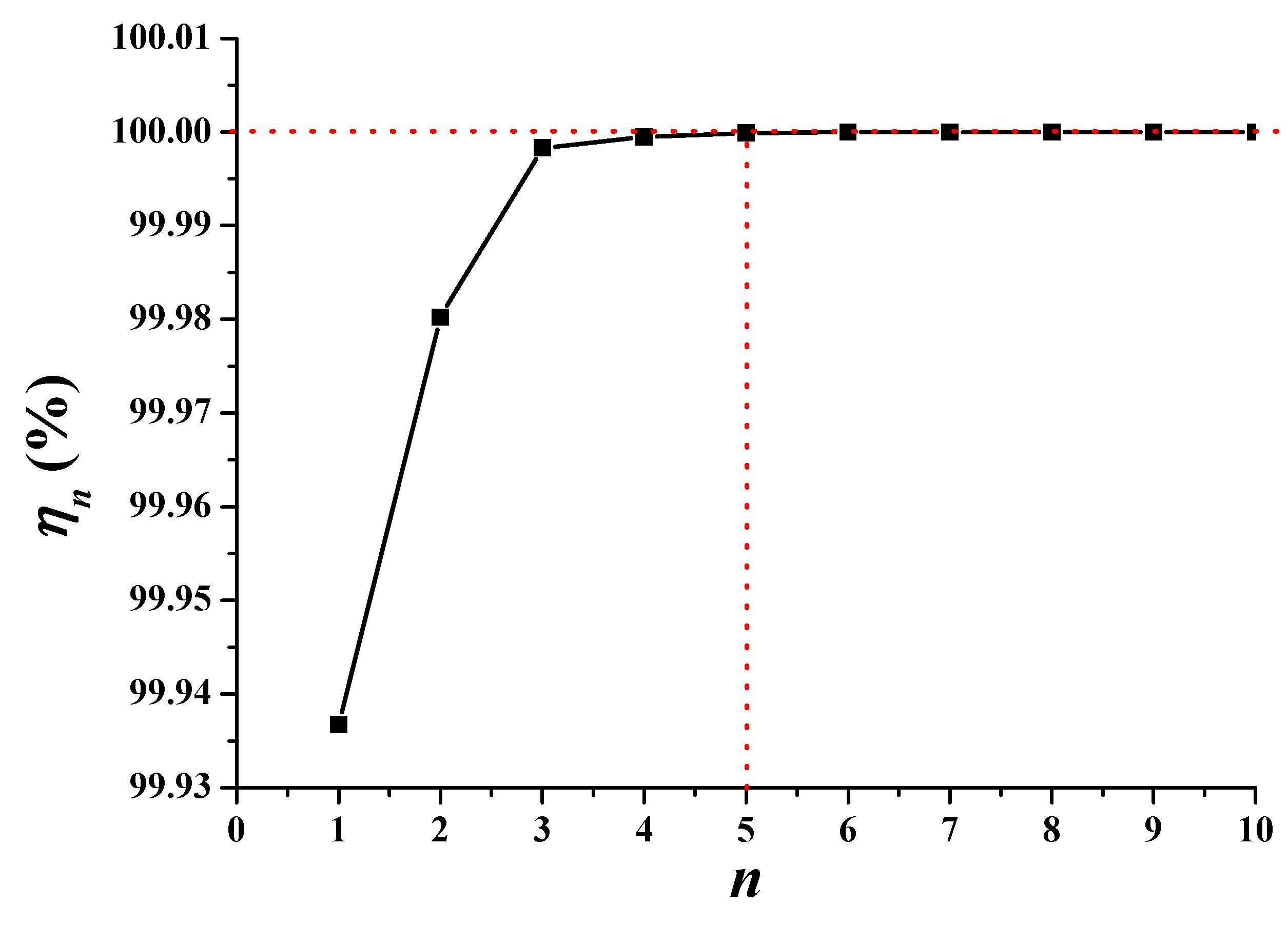
After the determination of the projection onto , the number of POD modes should also be determined because it affects the precision of the POD model. The importance of the mode number can be represented by the energy spectrum:
where is the cumulative energy contribution of the top n POD modes () to total energy. Once achieves 100%, it indicates that all information has been captured by these top n POD modes. As shown in Figure 6, the cumulative energy contribution achieves 100% from the 5th or 6th mode so that the POD modes at least after the 6th mode should be neglected. The exact mode number needs an examination of the relative error for the whole transient process.
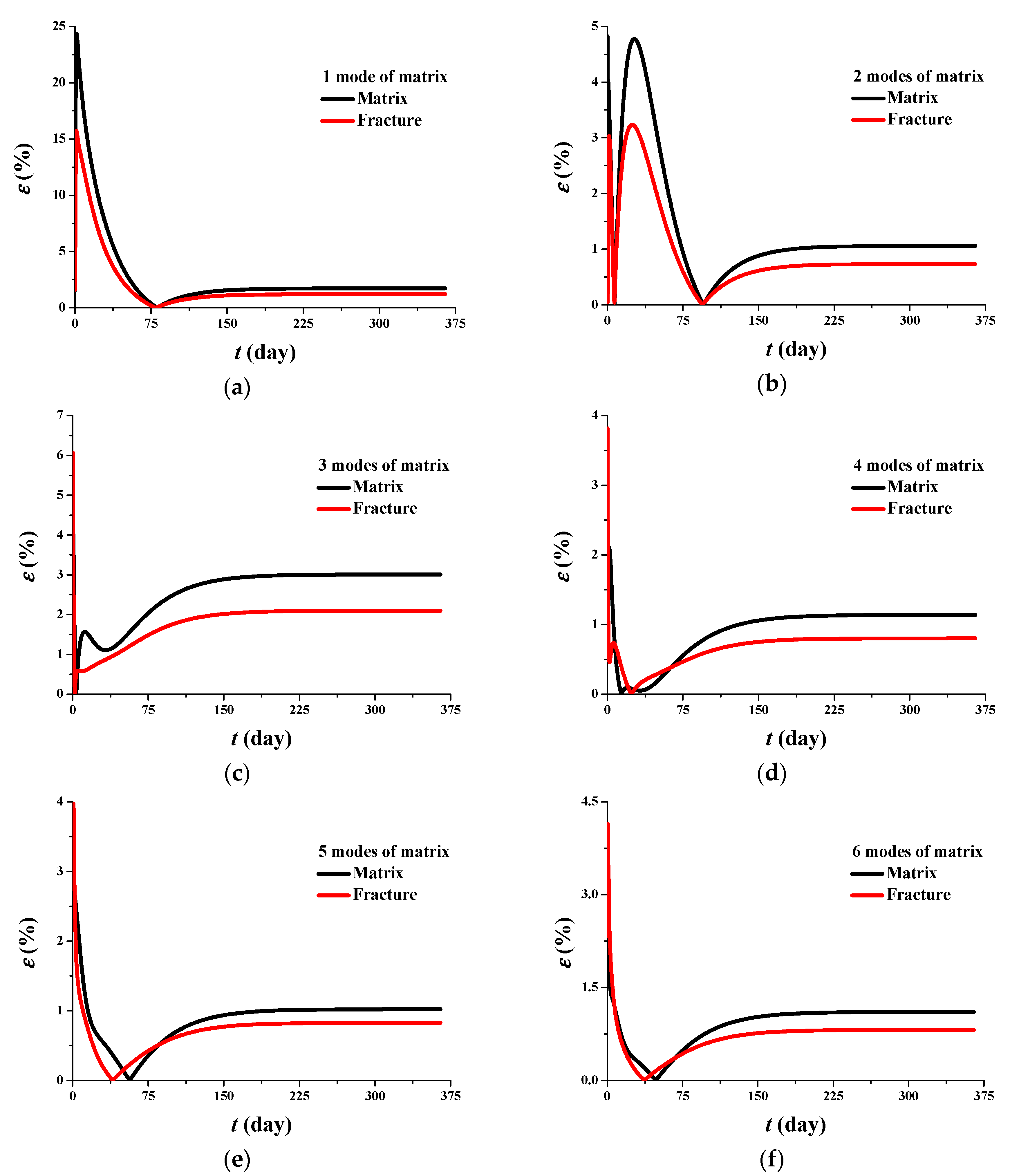
The temporal evolutions of relative errors using different POD modes are shown in Figure 7. Relative errors for the matrix and fracture pressures fluctuate at the initial stage and then rapidly decrease to a stable value at any number of POD modes. They decrease with increasing number of POD modes and become stable after five modes. The addition of the 6th mode causes the error to increase slightly (Figure 7f), indicating that the 6th mode has no positive contribution to precision promotion. Thus, the top five modes should be adopted in the new POD model.
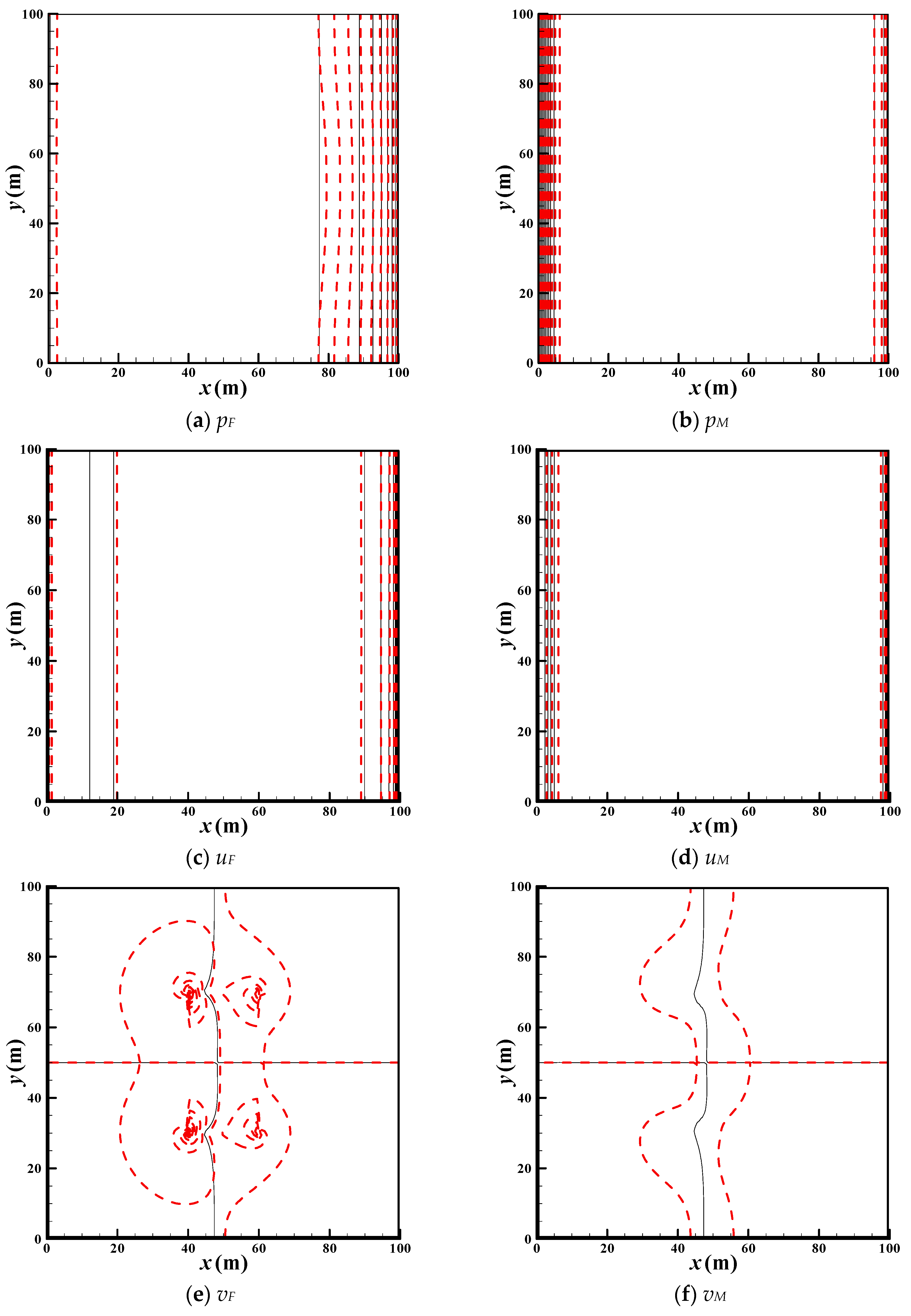
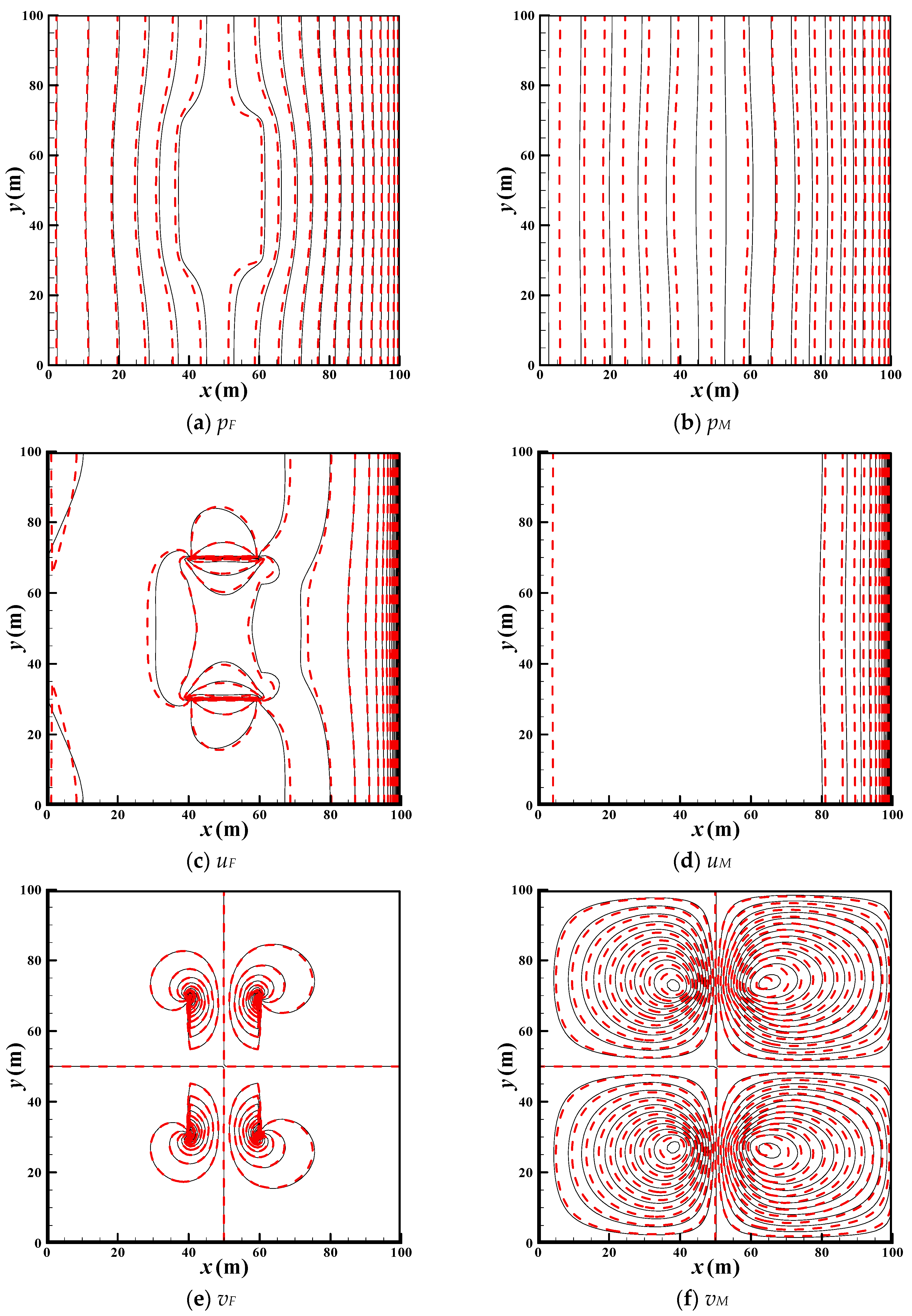
To further examine the local precision of the new POD model, it is necessary to compare the local flow fields at two typical moments (0.15 days and 365 days). At 0.15 days, the reconstruction errors of the POD are maximum. At 365 days, the reconstruction errors of the POD stay low and stable. As shown in Figure 8 and Figure 9, the reconstructed pressure fields and velocity fields in the fracture and matrix from the new POD model always agree well with those from FDM. The local distributions of the reconstructed flow fields by POD only have small deviations with the flow fields computed by FDM, regardless of whether the reconstruction errors are large (, at 0.15 days) or small (, at 365 days). Thus, it is confirmed that the new POD model can reproduce all the transient characteristics of pressure and velocity for gas flow in the dual-porosity, dual-permeability system with high precision.
The aim of POD modeling is not only high-precision reconstruction, but also a large-acceleration of computation. Hence, the verification of computational speed is important. The comparison of code running time, i.e., CPU time, is listed in Table 5. For the same period of simulation time (365 days in this case), simulation via FDM needs one hour (i.e., 3600 s), but the simulation via the new POD model only needs 5 s. The acceleration of computational speed is as high as 720 times, indicating that the computational time is largely saved. The new POD modeling approach is a good way to decrease CPU time for numerical computation for gas flow in dual-porosity, dual-permeability porous media.
4. Conclusions
POD modeling for gas flow in dual-porosity, dual-permeability porous media was studied for the purpose of the acceleration of computation with high-precision for potential engineering applications. Some conclusions related to the principle of POD modeling for this type of flow can be made as follows:
- (1)
- For dual-porosity, dual-permeability porous media, the typical method should be avoided to project the matrix equation and fracture equation separately. Otherwise, an artificial mass transfer term, which is 103~102 times larger than the diffusion term, will be generated to cause the failure of the POD modeling, because it violates the mass conservation of the whole system.
- (2)
- A mass conservation POD modeling method is proposed to ensure that no artificial mass transfer is generated by the POD projection process. Original governing equations should be projected onto the POD modes of matrix pressure to maintain a robust POD model.
- (3)
- The new POD model obeying the mass-conservation nature of the whole system can promote computational speed as much as 720 times under high precision: , ; , ; , .
Acknowledgments
The work presented in this paper has been supported by National Natural Science Foundation of China (NSFC) (No. 51576210, No. 51325603), Science Foundation of China University of Petroleum-Beijing (No. 2462015BJB03, No. 2462015YQ0409, No. C201602) and supported in part by funding from King Abdullah University of Science and Technology (KAUST) through the grant BAS/1/1351-01-01. This work is also supported by the Foundation of Key Laboratory of Thermo-Fluid Science and Engineering (Xi’an Jiaotong University), Ministry of Education, Xi’an 710049, P. R. China (KLTFSE2015KF01).
Author Contributions
Y.W. has contributed to the model derivation, coding, simulation, and preparation of the article; S.S. has contributed to the concept design and language polishing; B.Y. has contributed to the numerical methods.
Conflicts of Interest
The authors declare no conflict of interest.
References
- Wu, Y.S.; Haukwa, C.; Bodvarsson, G.S. A physically based approach for modeling multiphase fracture-matrix interaction in fractured porous media. Adv. Water Resour. 2004, 27, 875–887. [Google Scholar] [CrossRef]
- Wu, Y.S.; Lu, G.; Zhang, K.; Pan, L.; Bodvarsson, G.S. Analyzing unsaturated flow patterns in fractured rock using an integrated modeling approach. Hydrogeol. J. 2007, 15, 553–572. [Google Scholar] [CrossRef]
- Wu, Y.S.; Di, Y.; Kang, Z.; Fakcharoenphol, P. A multiple-continuum model for simulating single-phase and multiphase flow in naturally fractured vuggy reservoirs. J. Petrol. Sci. Eng. 2011, 78, 13–22. [Google Scholar] [CrossRef]
- Lin, D.; Wang, J.J.; Yuan, B.; Shen, Y.H. Review on gas flow and recovery in unconventional porous rocks. Adv. Geo-Energy Res. 2017, 1, 39–53. [Google Scholar]
- Wu, Y.S.; Qin, G. A generalized numerical approach for modeling multiphase flow and transport in fractured porous media. Commun. Comput. Phys. 2009, 6, 85–108. [Google Scholar] [CrossRef]
- Presho, M.; Wo, S.; Ginting, V. Calibrated dual porosity dual permeability modeling of fractured reservoirs. J. Petrol. Sci. Eng. 2011, 77, 326–337. [Google Scholar] [CrossRef]
- De Swaan, O.A. Analytical solutions for determining naturally fractured reservoir properties by well testing. SPE J. 1976, 16, 117–122. [Google Scholar] [CrossRef]
- Chen, Z.X. Transient flow of slightly compressible fluids through double-porosity double-permeability systems—A state-of-the-art review. Trans. Porous Med. 1989, 4, 147–184. [Google Scholar] [CrossRef]
- Huang, C.S.; Chen, Y.L.; Yeh, H.D. A general analytical solution for flow to a single horizontal well by fourier and laplace transforms. Adv. Water Resour. 2011, 34, 640–648. [Google Scholar] [CrossRef]
- Nie, R.S.; Meng, Y.F.; Jia, Y.L.; Zhang, F.X.; Yang, X.T.; Niu, X.N. Dual porosity and dual permeability modeling of horizontal well in naturally fractured reservoir. Transp. Porous Med. 2012, 92, 213–235. [Google Scholar] [CrossRef]
- Cai, J.; Hu, X.; Standnes, D.C.; You, L. An analytical model for spontaneous imbibition in fractal porous media including gravity. Colloids Surf. A 2012, 414, 228–233. [Google Scholar] [CrossRef]
- Chen, J.; Chen, Z. Three-dimensional superconvergent gradient recovery on tetrahedral meshes. Int. J. Numer. Methods Eng. 2016, 108, 819–838. [Google Scholar] [CrossRef]
- Wang, Y.; Yu, B.; Wu, X.; Wang, P. POD and wavelet analyses on the flow structures of a polymer drag-reducing flow based on DNS data. Int. J. Heat Mass Transf. 2012, 55, 4849–4861. [Google Scholar] [CrossRef]
- Wang, Y.; Yu, B.; Cao, Z.; Zou, W.; Yu, G. A comparative study of POD interpolation and POD projection methods for fast and accurate prediction of heat transfer problems. Int. J. Heat Mass Transf. 2012, 55, 4827–4836. [Google Scholar] [CrossRef]
- Wang, Y.; Yu, B.; Sun, S. Fast prediction method for steady-state heat convection. Chem. Eng. Technol. 2012, 35, 668–678. [Google Scholar] [CrossRef]
- Ghommem, M.; Calo, V.M.; Efendiev, Y. Mode decomposition methods for flows in high-contrast porous media: A global approach. J. Comput. Phys. 2014, 257, 400–413. [Google Scholar] [CrossRef]
- Wang, Y.; Yu, B.; Sun, S. POD-Galerkin model for incompressible single-phase flow in porous media. Open Phys. 2016, 14, 588–601. [Google Scholar] [CrossRef]
- Kazemi, H.; Merrill, L.S.; Porterfield, K.L.; Zeman, P.R. Numerical simulation of water-oil flow in naturally fractured reservoirs. SPE J. 1976, 16, 317–326. [Google Scholar] [CrossRef]
Figure 1.
Computational domain and boundary condition.

Figure 2.
Permeability fields: white region-100 md, black region-1 md (1 md = 9.8692327 × 10⁻¹⁶ m2). (a) Permeability of fracture; (b) Permeability of matrix.
Figure 2.
Permeability fields: white region-100 md, black region-1 md (1 md = 9.8692327 × 10⁻¹⁶ m2). (a) Permeability of fracture; (b) Permeability of matrix.

Figure 3.
Numerical errors of pressures in the matrix and fracture for typical POD modeling.

Figure 4.
Pressure fields comparison at t1: black solid line-FDM; red dashed line-POD. (a) Fracture (εF = 18.89%); (b) Matrix (εM = 16.26%).
Figure 4.
Pressure fields comparison at t1: black solid line-FDM; red dashed line-POD. (a) Fracture (εF = 18.89%); (b) Matrix (εM = 16.26%).

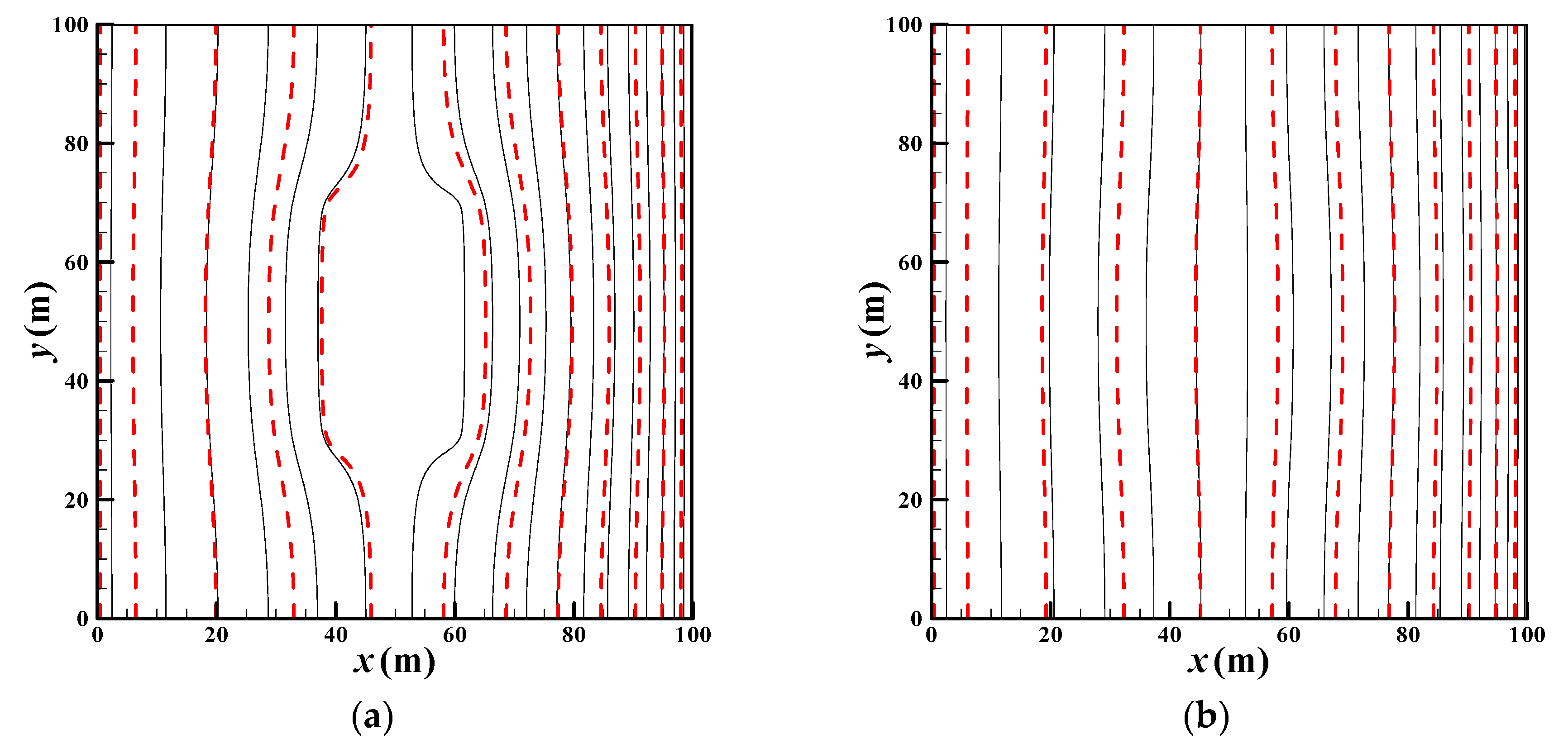
Figure 5.
Pressure fields comparison for typical POD modeling at t2: black solid line-FDM; red dashed line-POD. (a) Fracture (εF = 38.67%); (b) Matrix (εM = 38.98%).
Figure 5.
Pressure fields comparison for typical POD modeling at t2: black solid line-FDM; red dashed line-POD. (a) Fracture (εF = 38.67%); (b) Matrix (εM = 38.98%).

Figure 6.
Cumulative energy contribution of the top n POD modes.

Figure 7.
Relative errors of matrix and fracture pressures using the new POD modeling. (a) top 1 mode; (b) top 2 modes; (c) top 3 modes; (d) top 4 modes; (e) top 5 modes; (f) top 6 modes.
Figure 7.
Relative errors of matrix and fracture pressures using the new POD modeling. (a) top 1 mode; (b) top 2 modes; (c) top 3 modes; (d) top 4 modes; (e) top 5 modes; (f) top 6 modes.

Figure 8.
Flow field comparison for matrix and fracture at 0.15 days: black solid line-FDM; red dashed line-POD (, ).
Figure 8.
Flow field comparison for matrix and fracture at 0.15 days: black solid line-FDM; red dashed line-POD (, ).

Figure 9.
Flow field comparison for matrix and fracture at 365 days: black solid line-FDM; red dashed line-POD (, ).
Figure 9.
Flow field comparison for matrix and fracture at 365 days: black solid line-FDM; red dashed line-POD (, ).


Table 1.
Additional parameters for computation.
| Parameter | Value | Unit |
|---|---|---|
| 0.5 | / | |
| 0.02 | / | |
| 1,013,250 | Pa | |
| 1,013,250 | Pa | |
| 2,026,500 | Pa | |
| 101,325 | Pa | |
| 0 | Kg/(m3·s) | |
| 0 | Kg/(m3·s) | |
| 8.9177127 × 10⁻¹¹ | m2/(Pa·s) | |
| W | 16 × 10−3 | Kg/mol |
| R | 8.3147295 | J/(mol·K) |
| T | 298 | K |
| 11.067 × 10⁻⁶ | Pa·s | |
| nx | 100 | / |
| ny | 100 | / |
| Ns | 2433 | / |
| lx | 100 | m |
| ly | 100 | m |
| Lx | 0.2 | m |
| Ly | 0.2 | m |
| 1 | m | |
| 1 | m | |
| 1296 | s | |
| Simulation time scope | 365 | days |
Table 2.
Magnitude comparison between the net mass transfer and the diffusion term.
| N | 1 | 2 | 3 |
|---|---|---|---|
| −3.62 × 10² | −1.98 × 10³ | 4.85 × 10³ |
Table 3.
Time-averaged error of matrix pressure for different projection operators.
| (%) | N = 1 | N = 2 | N = 3 | N = 4 | N = 5 | N = 6 |
|---|---|---|---|---|---|---|
| Project onto | 2.7527 | 1.3319 | 2.5884 | 0.9123 | 0.8826 | 0.9110 |
| Project onto | 2.7469 | 1.8863 | 1.9840 | 1.1248 | N/A | N/A |
Table 4.
Time-averaged error of fracture pressure for different projection operators.
| (%) | N = 1 | N = 2 | N = 3 | N = 4 | N = 5 | N = 6 |
|---|---|---|---|---|---|---|
| Project onto | 1.9049 | 0.9131 | 1.8079 | 0.6702 | 0.7182 | 0.7062 |
| Project onto | 1.8990 | 1.3435 | 1.3795 | 0.7912 | N/A | N/A |
Table 5.
Acceleration ability of the new POD model.
| FDM | New POD Model | |
|---|---|---|
| CPU time | 3600 s | 5 s |
© 2017 by the authors. Licensee MDPI, Basel, Switzerland. This article is an open access article distributed under the terms and conditions of the Creative Commons Attribution (CC BY) license (http://creativecommons.org/licenses/by/4.0/).
Share and Cite
MDPI and ACS Style
Wang, Y.; Sun, S.; Yu, B. Acceleration of Gas Flow Simulations in Dual-Continuum Porous Media Based on the Mass-Conservation POD Method. Energies 2017, 10, 1380. https://0-doi-org.brum.beds.ac.uk/10.3390/en10091380
AMA Style
Wang Y, Sun S, Yu B. Acceleration of Gas Flow Simulations in Dual-Continuum Porous Media Based on the Mass-Conservation POD Method. Energies. 2017; 10(9):1380. https://0-doi-org.brum.beds.ac.uk/10.3390/en10091380
Chicago/Turabian StyleWang, Yi, Shuyu Sun, and Bo Yu. 2017. "Acceleration of Gas Flow Simulations in Dual-Continuum Porous Media Based on the Mass-Conservation POD Method" Energies 10, no. 9: 1380. https://0-doi-org.brum.beds.ac.uk/10.3390/en10091380
Note that from the first issue of 2016, this journal uses article numbers instead of page numbers. See further details here.