Lattice Boltzmann Simulation of Fluid Flow Characteristics in a Rock Micro-Fracture Based on the Pseudo-Potential Model

Faculty of Civil Engineering and Mechanics, Kunming University of Science and Technology, Kunming 650500, China
*
Author to whom correspondence should be addressed.
Energies 2018, 11(10), 2576; https://0-doi-org.brum.beds.ac.uk/10.3390/en11102576
Submission received: 9 August 2018
/
Revised: 25 September 2018
/
Accepted: 26 September 2018
/
Published: 27 September 2018
(This article belongs to the Special Issue Flow and Transport Properties of Unconventional Reservoirs 2018)
Abstract
:Slip boundary has an important influence on fluid flow, which is non-negligible in rock micro-fractures. In this paper, an improved pseudo-potential multi-relaxation-time (MRT) lattice Boltzmann method (LBM), which can achieve a large density ratio, is introduced to simulate the fluid flow in a micro-fracture. The model is tested to satisfy thermodynamic consistency and simulate Poiseuille flow in the case of large liquid-gas density ratio. The slip length is used as an index for evaluating the flow characteristics, and the effects of wall wettability, micro-fracture width, driving pressure and liquid-gas density ratio on the slip length are discussed. The results demonstrate that the slip length increases significantly with the increase of the wall contact angle in rock micro-fracture. And the liquid-gas density ratio has an important impact on the slip length, especially for the hydrophobic wall. Moreover, under the laminar flow regime the driving pressure and the micro-fracture width has little effect on the slip length.
1. Introduction
The fluid flow in rock micro-fractures is a topic of great importance for a wide range of scientific problems, such as water conservancy, oil recovery in low-permeability oilfields, nuclear waste treatment and others [1,2,3,4]. Classical Navier-Stokes hydrodynamics with non-slip boundaries, in which the fluid velocity at a fluid-solid interface equals the solid velocity, is successfully applied to seepage research at the macro-scale. However, a series of experimental and numerical results indicate that the non-slip boundary notion is invalid at the micro-scale [5,6]. Besides, there are a large number of micro-fractures in the rock with the width < 1 mm [7]. The slip boundaries should be taken into account during the fluid flow in these micro-fractures [8,9]. Meanwhile, the surfaces of micro-fractures show different wettabilities due to its diverse mineral composition [10], and it has a strong influence on the wall slip. Therefore, great attention should be paid to studying the slip conditions in micro-fractures with different wettabilities.
Slip length is an important dynamic parameter for quantifying the slip condition of a liquid flowing over the solid surface, and it’s difficult to measure directly through experiments due to the objective limits of the current techniques [11,12]. Thus, slip length studies in micro-fluidics have focused on numerical simulations. The lattice Boltzmann method (LBM) offers great potential for micro-scale flow simulations owing to its mesoscopic particle background [13]. Many scholars have studied micro-scale fluid flow with the LBM and proposed several typical multiphase models, such as the color model, the free-energy model, the pseudo-potential model, etc. Among these, the pseudo-potential model realizes the phase separation by implementing micro-molecular interactions. It has received considerable attention due to the fact the interface between different phases does not need to be tracked or captured. Based on this model, Zhang et al. [14] found that the non-slip boundary conditions could produce an apparent slip. Chen et al. [15] simulated the Couette flow and found that there was a direct relationship between the magnitude of slip length and the strength of solid-fluid interaction. Zhang et al. [16] investigated the droplet flow velocity in the micro-channels, and discussed the wall slip caused by the roughness. Kunert [17] studied the influence of fluid viscosity on the slip length. However, almost all the studies do not consider the effect of liquid-gas density ratio on the wall slip due to the difficulty of achieving a large liquid-gas density ratio with the original pseudo-potential model [18].
Based on the LBM, an improved pseudo-potential model is introduced to simulate the liquid flow in a rock micro-fracture, which could achieve a large liquid-gas density ratio. The validity of the proposed model is tested on two benchmark cases: the thermodynamic consistency and Poiseuille flow. The slip length is discussed considering the effects of wall wettability, micro-fracture width, driving pressure and liquid-gas density ratio.
2. Slip Condition
Bernoulli first proposed the non-slip boundary model (Figure 1a) where the fluid velocity was zero relative to the physical wall. Subsequently, some scholars have supposed that the fluid layer near the wall has a certain thickness (Figure 1b), in which no relative movement occurs between the fluid and the wall. In addition, some experimental results indicated that the fluid velocity was not zero at the wall (Figure 1c). The above three slip conditions have been confirmed, and they are deemed to be related to the wall wettability. When the fluid flow over a strong hydrophilic wall, it presents non-slip or negative slip, and a fluid usually shows a positive slip condition at a strong hydrophobic wall. As shown in Figure 1c, based on the assumption that the distance to the virtual wall, at which the extrapolated fluid velocity at a constant shear would be equal to the wall velocity, Navier defined the slip length as:
where is the slip velocity at the physical wall; is the local shear near the physical wall.
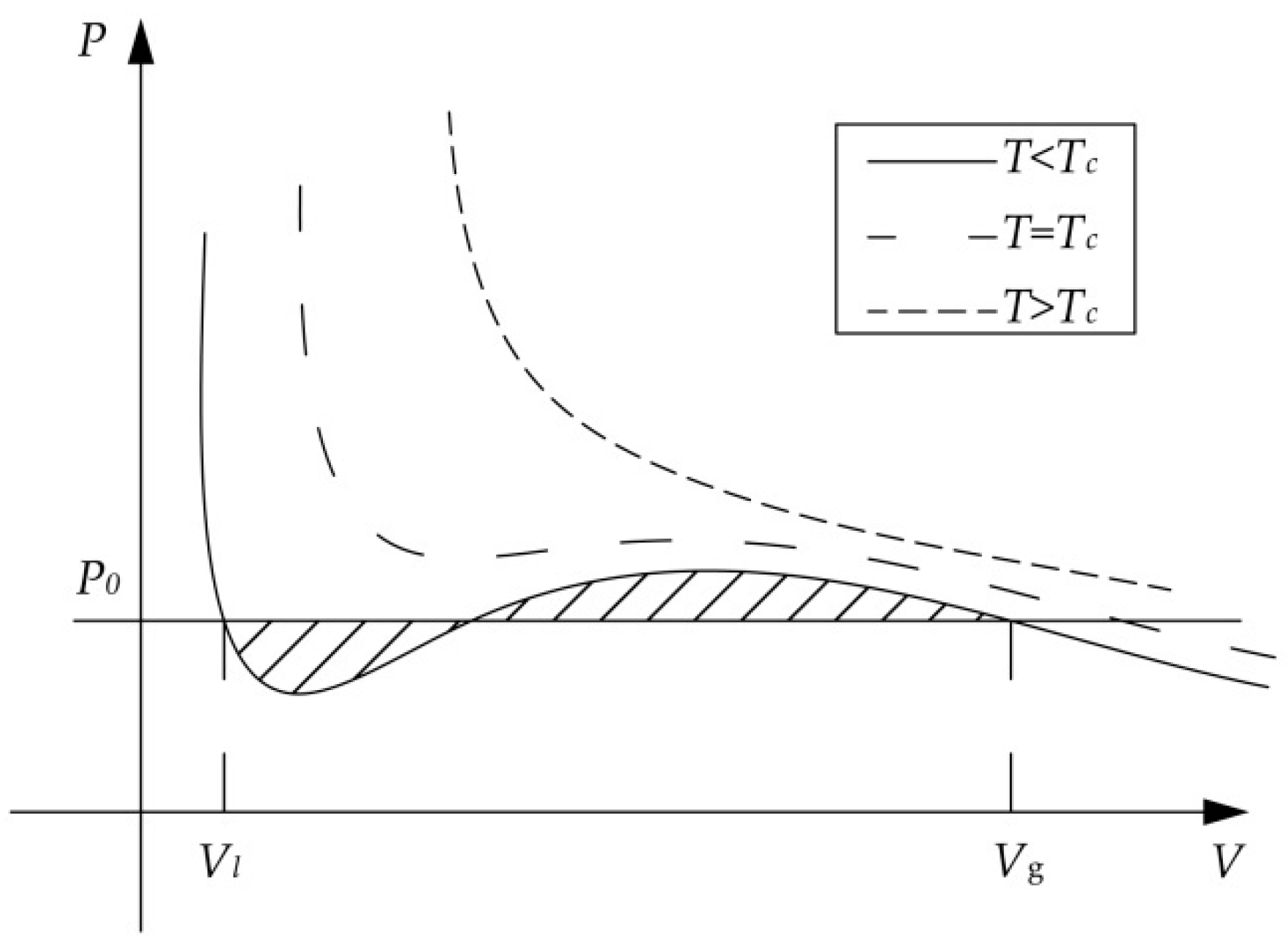
3. Coexistence Densities and Maxwell Construction Rule
In nature, the fluids in rock micro-fractures are mostly in a liquid-gas two phase situation. A two phase fluid could be described by its equation of state, which is an equation relating the fluid state variables in thermodynamics, such as pressure , molar volume , and temperature . Figure 2 shows a series of − curves of an equation of state with different temperatures, where the bulk (the region not close to any interface) pressure is a function of the molar volume and the temperature . For different temperatures, the fluid may show subcritical, critical, and supercritical behaviors. At high temperature (above the critical temperature ) the fluid shows supercritical behavior and no distinct liquid and gas phases can be discerned. Below the critical temperature, phase separation into liquid and gas is possible, and different molar volumes and of the certain substance may coexist at a single pressure at equilibrium, where and are the liquid and gas phases molar volumes, respectively. At the critical temperature, the coexistence of different molar volumes is also impossible, nevertheless the first and second derivative of at should be zero [19]:
The Carnahan-Starling equation of state (C-S EOS) is one of classic equations of state for non-ideal fluid, which is given by [19]:
where is the attraction parameter; is the repulsion parameter; is the gas constant and is the fluid density. Rearranging and taking the derivatives of Equation (3), and can be presented as function of the critical pressure and the :
Then, can be given as:
In this paper, the parameters in Equation (3) are set as , , , respectively [20]. Then . The reduced temperature coefficient () is introduced to ensure the temperature below the critical temperature, which makes the system at the subcritical behavior. The coexistence of different molar volumes at a single pressure could be found according to Maxwell construction rule [13]:
Replacing the molar volume as the reciprocal of density , Maxwell construction rule Equation (6) can be rewritten as:
where and are the liquid and gas phase coexistence densities, respectively. A series of coexistence densities with different temperatures could be directly obtained by numerical method according to Maxwell construction rule.
4. Numerical Model
4.1. The MRT-LBM
Using the Guo’s force scheme [21], the evolution equation of LBM can be given as follows:
where is the density distribution function in the direction; represents the coordinate of the node; is the discrete velocity; is the time step; is the collision operator; is the forcing term.
For the D2Q9 model:
The single-relaxation-time lattice Boltzmann method (SRT-LBM) can simplify the collision operator of the Equation (8). However, it comes at a cost of reduced accuracy and stability. Compared with SRT-LBM, the multi-relaxation-time lattice Boltzmann method (MRT-LBM), which offers a series of relaxation-time can overcome these problems [22]. So the MRT-LBM is applied in the present work. The collision operator and the Guo’s forcing term are respectively given by [23]:
where is an orthogonal transformation matrix; is a diagonal matrix; is the equilibrium density distribution function; is the forcing term in the moment space; and is the row and column number of a matrix, respectively. For the D2Q9 model, and can be written as:
where contains all the relaxation rates; it is set as [20] in this paper. The kinematic viscosity can be derived from one of the relaxation coefficients : , where is lattice sound speed, and is the lattice constant, which is set as 1 for the present.
The moments can be obtained by ; the equilibrium moments can be straightforwardly computed by . Alternatively, it can be constructed more precisely and efficiently from the density and the velocity by [20]:
where is the macroscopic velocity given by ; and is the macroscopic density; is the total force.
Through Equations (11) and (12), the Equation (8) can be transformed as follows:
where are the moments after the collision step; is the unit tensor; is the forcing term in the moment space which is given by [20]:
After the collision step, the moments should be transformed to the density distribution function by , then the can be streamed to the next node through Equation (9).
4.2. The Original Pseudo-Potential Model
The total force in Equation (17) is given by , where is the external force such as gravitational force and buoyancy force. The inter-molecular force can be obtained by the pseudo-potential presented in the following, which is a function to mimic the molecular interactions that cause phase separation. is the inter-molecular force within fluids; is the adhesive force between fluid particles and solid wall. Both and can be expressed as [24,25,26]:
where is the interaction strength, which is set as 6.0 in the present paper; is the weight, and ; represents the solid wall node; is the wall density. It should be noticed that is not a real physical density. It is merely an artificial parameter to acquire different wall affinities.
Using the Chapman-Enskog analysis, the following macroscopic equation can be derived from Equations (11), (15)–(17) [20]:
Combining Equations (21) and (22), the normal pressure tensor of the interface can be given by [26]:
where the subscript n denotes the normal direction of the interface; and are constants for the D2Q9 model. According to Equation (23) and the physical requirement that the interface pressure should be equal to the bulk (the region not close to any interface) pressure at equilibrium, the following mechanical stability condition can be written as:
where , , and . In the pseudo-potential LB model, the coexistence densities ( and ) are determined by the mechanical stability condition Equation (24). Maxwell construction rule, which determines the thermodynamic coexistence, is built in the requirement of Equation (7). To satisfy the Equation (7), Sbragaglia and Shan [28] have proposed the following interaction potential :
which gives . With the above potential function, Equations (7) and (22) will be same, thereby the thermodynamic consistency (Maxwell construction rule) will be obtained. But, to be consistent with the equation of state in the thermodynamic theory, the potential must be chosen as [18,29]:
Obviously, Equations (25) and (26) cannot be obtained at the same time, so this original pseudo-potential model cannot content the thermodynamic consistency.
4.3. The Improved Pseudo-Potential Model
To resolve the problem of thermodynamic inconsistency, the parameter in Equation (24) can be tuned to approximately achieve the thermodynamic consistency when is defined by Equation (26). Through changing the original forcing term, Equation (17) is rewritten as follows [20]:
Meanwhile, Equation (23) could be given as:
which leads to , where is a correction parameter which could tune the mechanical stability condition Equation (24) to approximately get the thermodynamic consistency.
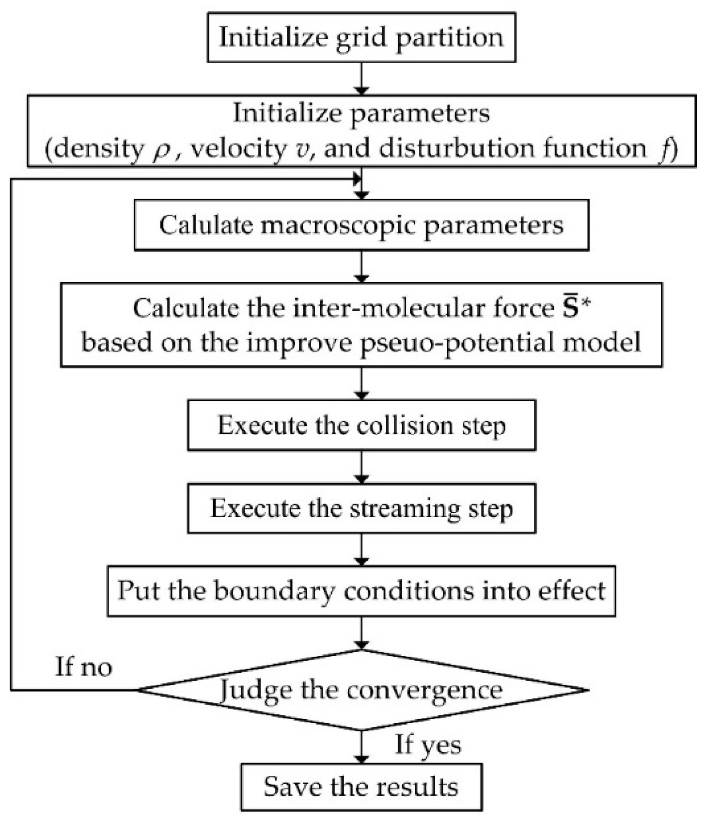
4.4. Flowchart of the MRT-LBM
Based on the improved pseudo-potential model, the MRT-LBM has been proposed to simulate the fluid flow in the rock micro-fracture. The flowchart is shown in Figure 3.
4.5. Verification
Two reference problems are simulated to verify the improved pseudo-potential MRT-LBM in this section. One case is a bubble in gas, which is applied to test the thermodynamic consistency with large liquid-gas density ratio. The other is Poiseuille flow, in which the slip boundary with the slip length close to zero is applied to simulate the non-slip behavior. It should be noticed that the units in this paper are all lattice units.
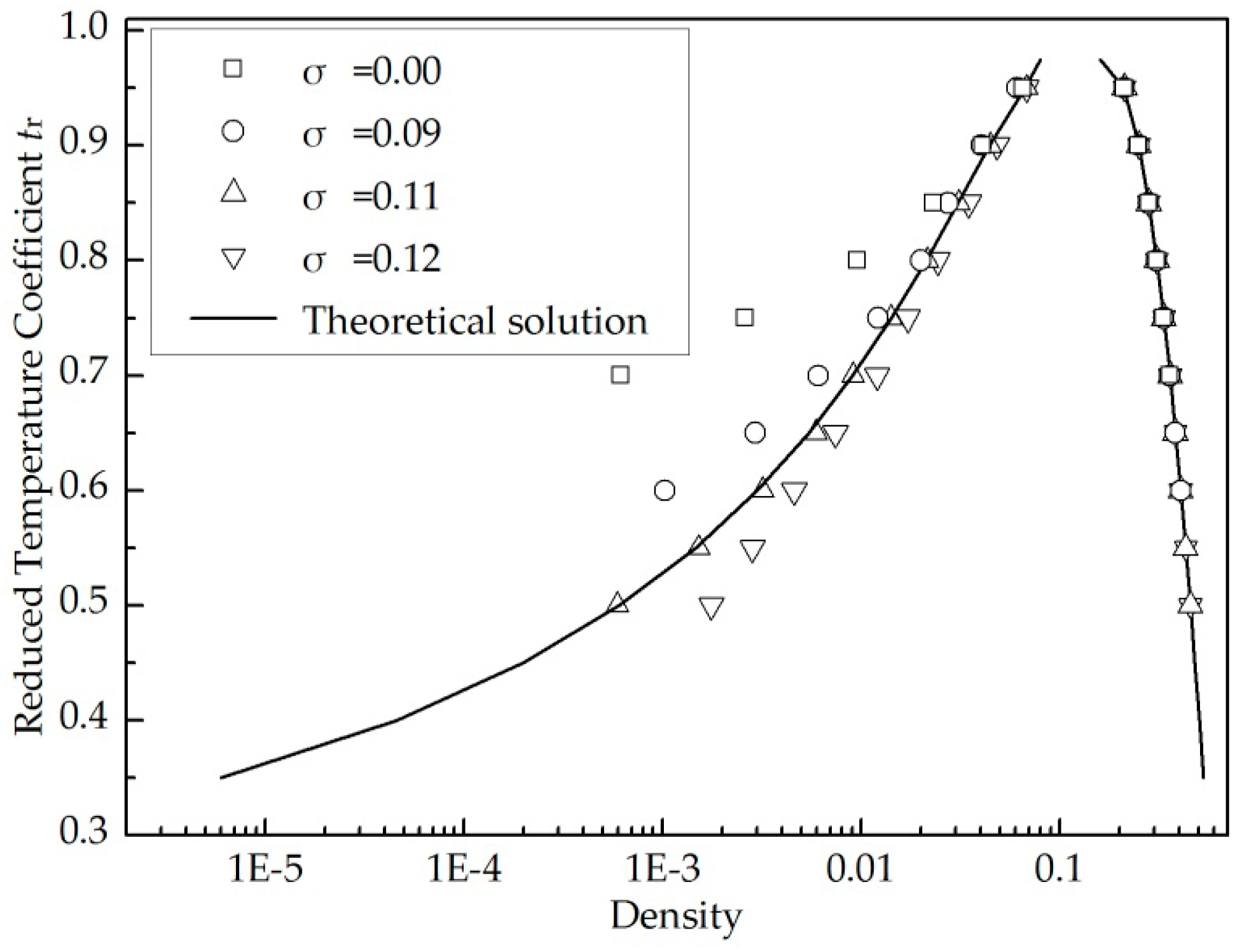
4.5.1. The Thermodynamic Consistency
A bubble in gas is simulated in a 100 × 100 lattice computational domain. The periodic boundary is set for its four sides, and the bubble is placed in the middle. The liquid-gas density coexistence curves are obtained by changing the temperature , which are compared with the theoretical curve given by Maxwell construction rule [30]. As shown in Figure 4, the results of the original forcing scheme (), and the improved model with are in good agreement with the theoretical results in the liquid phase, but there are large deviation between them in the gas phase. The numerical solutions of the improved forcing scheme with agrees well with the theoretical ones in both phases, which indicate that the proposed model could satisfy the thermodynamic consistency in the case of large liquid-gas density ratio, so the correction parameter is set as 0.11 in the following work.
4.5.2. Poiseuille Flow
Poiseuille flow is simulated with the slip length close to zero (). A 800 × 100 uniform lattice system is chosen in this case, the top and bottom boundaries are solid walls with the bounce-back boundaries, and the left and right sides are set as the periodic boundaries. To analyze the influence of different discretization features, we simulate the Poiseuille flow with the different mesh sizes (400 × 50, 800 × 100, and 1600 × 200). In this test, the liquid kinematic viscosity is 0.1, the liquid is driven by the pressure of 3 × 10⁻⁴ along the horizontal direction. The wall density is set as 0.12 to ensure the slip length close to zero (). The reduced temperature coefficient is 0.55. The correction parameter is 0.11. Other parameters are set as follows: lattice spaces are equal in horizontal and vertical direction, , and the time step is . Figure 5 shows the velocity profile obtained by the proposed model, which are compared with the theoretical solutions of Poiseuille flow (non-slip behavior) [13]. It is obvious that the fluid velocity given by numerical method shows a good match with the theoretical results and the grids number have little influence on the computed result. The maximum error is less than 3.24%. Hence, the improved pseudo-potential MRT-LBM can be used to simulate the fluid flow in the narrow channel successfully.
5. Results and Discussion
In the present study, the slip condition is discussed in a rock micro-fracture with different wettabilities. The wall wettability is the macroscopic expression of the interaction between fluid particles and the solid wall, so the relationship between the contact angle and the wall density is tested based on the improved the improved pseudo-potential model and the slip length, as an important parameter for judging the slip condition, is investigated considering the effects of contact angle, driving pressure, and liquid-gas density ratio.
5.1. Contact Angle Test
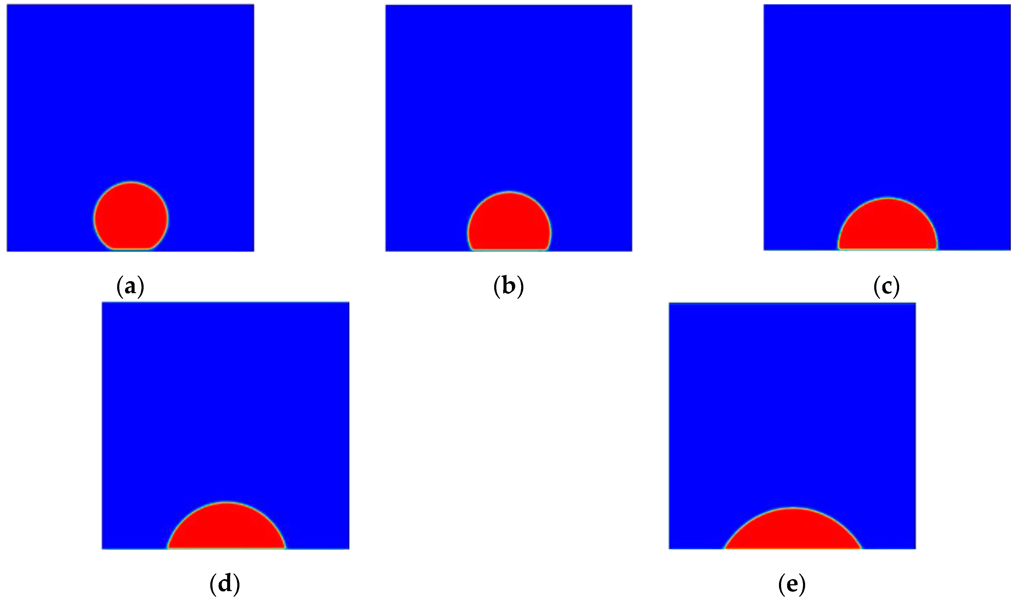
To obtain the relationship between the contact angle and the wall density, a 200 × 200 lattice domain is used, the top and bottom boundaries are solid walls and the left and right sides are set as the periodic boundaries. A liquid droplet is placed at the solid surface. The liquid-gas density ratio is set as 293:1 in this test. Different wall densities are applied to describe the changing wall affinities, Figure 6 presents different contact angles, and the relationship between the contact angle and the wall density is listed in Table 1.
5.2. Discussion
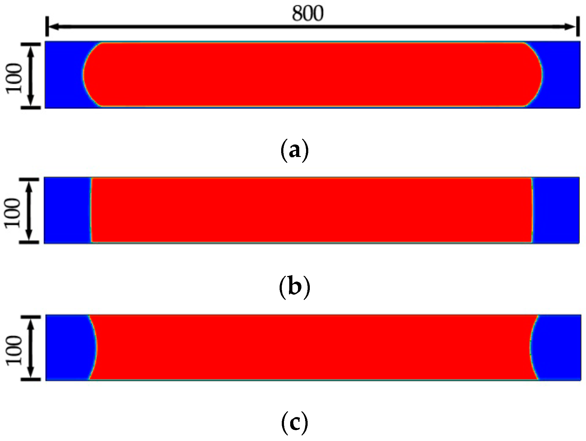
Based on the improved pseudo-potential MRT-LBM, a size of 800 × 100 lattice domain is applied to simulate the rock micro-fracture with different wettabilities. As shown in Figure 7, the left and right sides of the micro-fracture are set as the periodic boundaries; the top and bottom of the model are the solid walls. The volume ratio of liquid to gas is 9:2 in the initial state, and the liquid phase is placed in the middle of the micro-fracture. To ensure a laminar flow regime, the driving pressure of 3 × 10⁻⁴ is applied in the horizontal direction after the liquid-gas phases separated, in which the calculated Reynolds number is 1.49. The slip length, as an important parameter for judging the slip degree, is used to discuss the effects of contact angle, driving pressure, and liquid-gas density ratio on the fluid flow state in the micro-fracture.
5.2.1. Effect of the Contact Angle
In order to study the effect of the contact angle on the slip length, the liquid-gas density ratio is set as 293:1, and the micro-fracture widths are set as 25, 50, and 100, respectively. Figure 8 shows the slip length against the contact angle.
It can be observed that the slip length increases from −0.27 to 4.9 as the contact angle increasing from 61.9° to 148.7°. The larger the contact angle, the more significant the slip length changes. This finding is in agreement with that by Tsu-Hsu Yen [31] and Bladimir Ramos-Alvarado [32]. Moreover, in the case of different fracture widths, the variation trends of slip length with the contact angle are very close to each other, which indicate that the micro-fracture width has little effect on the slip length.
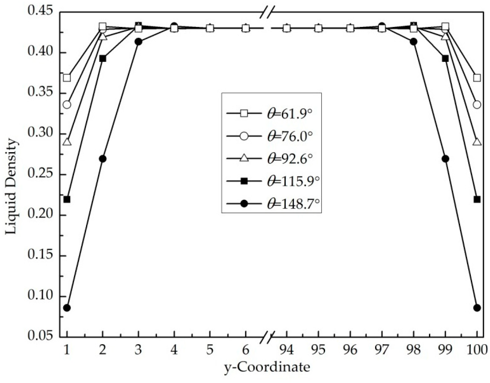
To analyze the physical mechanism of wall slip, the liquid density profiles (the fracture width is 100) for different contact angles are shown in Figure 9. As the contact angle increases, the liquid density near the wall decreases and the slip length increases, which confirms the existing slip theory [33,34]. The wall slip is induced by the changes of the liquid density near the solid surface, which is attributed to the varying interaction force between the liquid and the solid wall. With the increases of interaction force, the liquid density near the wall increases. Thereby it shows non-slip or even negative slip behaviors. As the interaction force decreases, the liquid density close to the wall surface decreases and the slip length increases. Even when the liquid density is less than a certain value, the liquid density near the wall surface is reduced to the gas density, so that a “gas layer” is formed at the solid surface.
5.2.2. Effect of the Driving Pressure
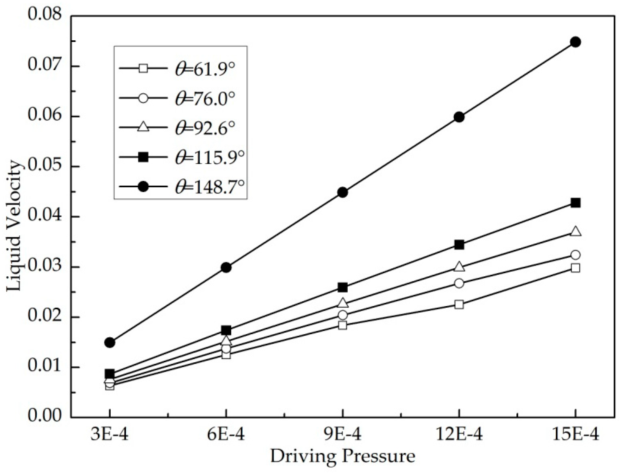
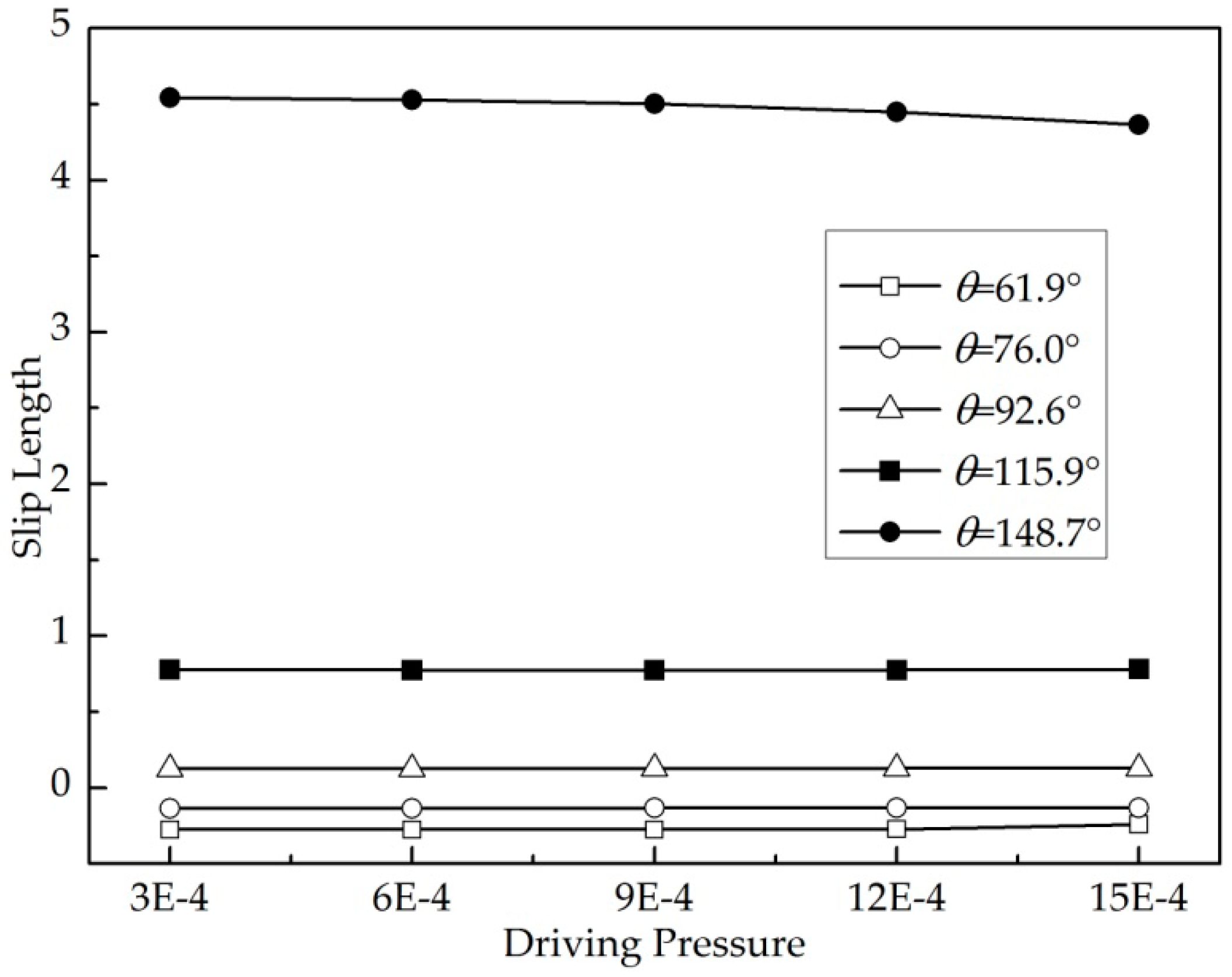
To investigate the effect of the driving pressure on the slip length, the micro-fracture width W is set as 100, the liquid-gas density ratio is 293:1, and the contact angles are 61.9°, 76.0°, 92.6°, 115.9° and 148.7°, respectively. When the driving pressure ranges from 3 × 10⁻⁴ to 1.5 × 10⁻³, the maximum Reynolds number is 7.48, which shows that the liquid flow is in a laminar flow regime. Figure 10 presents the relationship between the driving pressure and the average flow velocity, which indicates that the flow velocity linearly increases with the driving pressure. In Figure 11, the relationship between the driving pressure and the slip length shows that the driving pressure has almost no influence on the slip length. Xiang [35] and Huang [36] have also yielded the similar results by other numerical methods.
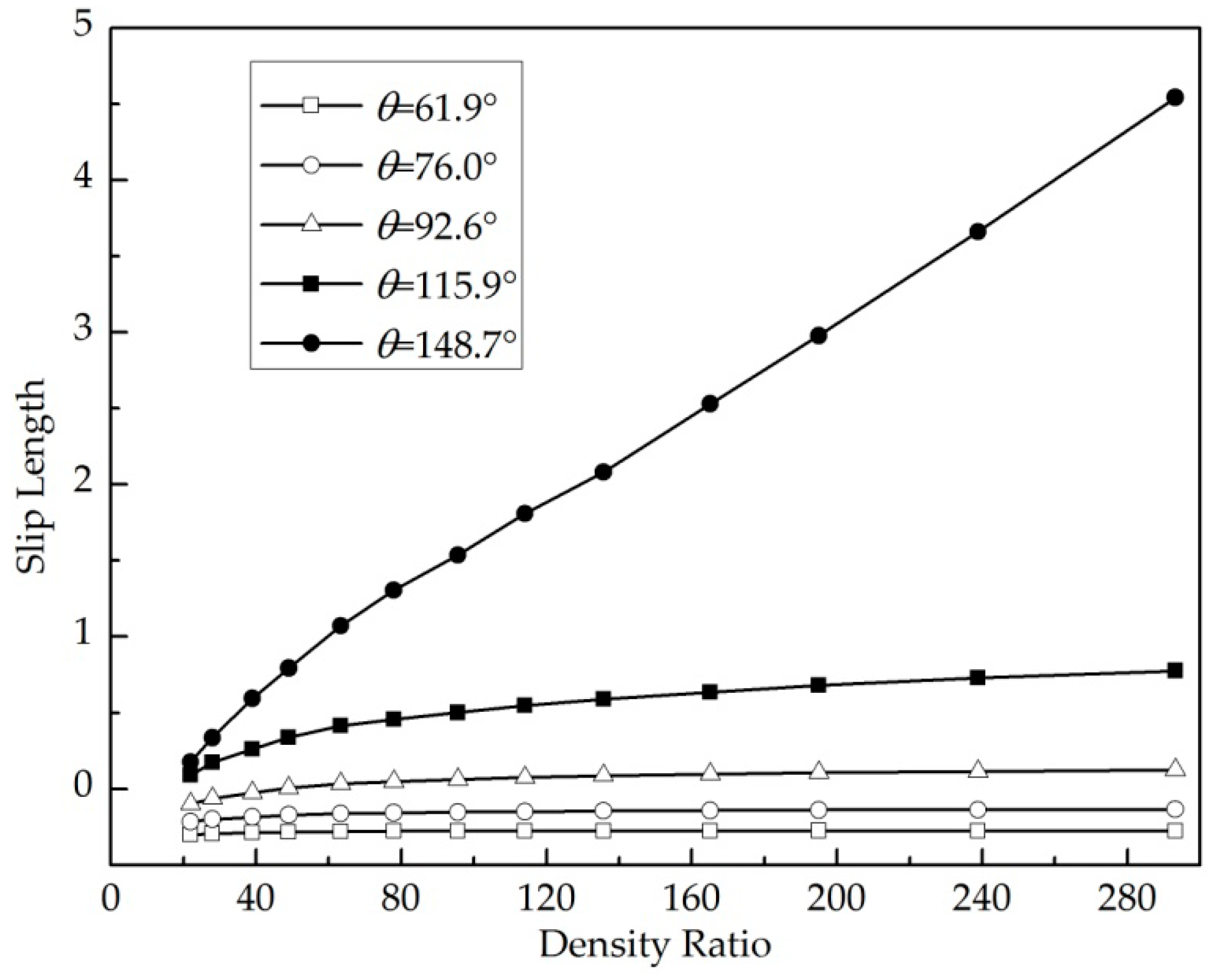
5.2.3. Effect of the Liquid-Gas Density Ratio
To study the influence of liquid-gas density ratio on the slip length, the liquid-gas density ratios are chosen in the range from 22:1 to 293:1. In this case, the micro-fracture width is 100, the driving pressure is 3 × 10⁻⁴, and the contact angles are 61.9°, 76.0°, 92.6°, 115.9°, and 148.7°, respectively. It should be noticed that changing liquid-gas density ratio will affect the contact angle, so the wall density should be lightly tuned to ensure the contact angle unchanged. Numerical results of the slip length against the density ratio are shown in Figure 12. In the case of , the slip length increases from 0.18 to 4.54 with the liquid-gas density ratio from 22:1 to 293:1. The relationship between the slip length and the density ratio is close to linear. The above phenomena is induced by the strong changes of the liquid density near the wall and the formation of the “gas layer” at the solid surface. When the contact angles are 115.9°, 92.6°, 76.0°, and 61.9°, the slip lengths increase from 0.09 to 0.77, −0.09 to 0.12, −0.21 to −0.13, and −0.30 to −0.27, respectively, the growth slope is relatively smaller. Thus, the liquid-gas density ratio has an important influence on the fluid flow characteristics, especially for the hydrophobic wall.
6. Conclusions
Based on the improved pseudo-potential model, the MRT-LBM is proposed to investigate the fluid flow in the rock micro-fracture, and it is verified according to two benchmark cases. The slip length is used to evaluate the flow characteristics in the micro-fracture, and the effects of the contact angles, the driving pressure, and the liquid-gas density ratio on the slip length are discussed, the corresponding conclusions are summarized as follows:
- (1)
- With increasing contact angle, the slip length increases at the wall, and the larger the contact angle, the more obvious the slip length changes.
- (2)
- Under the laminar flow regime, the fluid flow velocity is proportional to the driving pressure, but there is almost no change in the slip length with the driving pressure increasing, so the driving pressure has almost no impact on the slip length.
- (3)
- The slip length increases with the increasing of the liquid-gas density ratio, and the larger the wall contact angle, the more remarkable it shows. The liquid-gas density ratio has an important influence on the fluid flow characteristics, especially for the hydrophobic wall.
- (4)
- The wall slip is induced by the changing of liquid density near the solid surface, which is attributed to the varying interaction force between fluid particles and the solid wall. With the decrease of interaction force, the liquid density near the wall decreases and the slip length increases.
And as the increase of interaction force, it shows no slip or even negative slip at the solid wall.
Author Contributions
Each author has made contributions to the present paper. W.Z. proposed this topic and designed the calculation verification. P.W. performed the simulation and the result analysis. General supervision was provided by L.S. L.X. provided simulation support. All authors have read and approved the final manuscript.
Funding
This research was funded by the National Natural Science Foundation of China (No. 51508253, 51668028) and the Yunnan Applied Basic Research Project (No. 2016FB077).
Conflicts of Interest
The authors declare no conflict of interest.
References
- Wang, F.; Liu, Y.; Hu, C.; Shen, A.; Liang, S.; Cai, B.; Sciubba, E. A simplified physical model construction method and gas-water micro scale flow simulation in tight sandstone gas reservoirs. Energies 2018, 11, 1559. [Google Scholar] [CrossRef]
- Zhu, W.; Li, B.; Liu, Y.; Song, H.; Wang, X. Solid-liquid interfacial effects on residual oil distribution utilizing three-dimensional micro network models. Energies 2017, 10, 2059. [Google Scholar] [CrossRef]
- Di, Q.; Shen, C.; Wang, Z.H. Experimental research on drag reduction of flow in micro channels of rock using nano-particle adsorption method. Acta Pet. Sin. 2009, 30, 125–128. [Google Scholar]
- Coli, N.; Pranzini, G.; Alfi, A.; Boerio, V. Evaluation of rock-mass permeability tensor and prediction of tunnel inflows by means of geostructural surveys and finite element seepage analysis. Eng. Geol. 2008, 101, 174–184. [Google Scholar] [CrossRef]
- Voronov, R.S.; Papavassiliou, D.V.; Lee, L.L. Slip length and contact angle over hydrophobic surfaces. Chem. Phys. Lett. 2007, 441, 273–276. [Google Scholar] [CrossRef]
- Burton, Z.; Bhushan, B. Hydrophobicity, adhesion, and friction properties of nanopatterned polymers and scale dependence for micro-and nanoelectromechanical systems. Nano Lett. 2005, 5, 1607. [Google Scholar] [CrossRef] [PubMed]
- Hanna, R.B.; Rajaram, H. Influence of aperture variability on dissolutional growth of fissures in Karst Formations. Water Resour. Res. 1998, 34, 2843–2853. [Google Scholar] [CrossRef] [Green Version]
- Cao, B.Y.; Chen, M.; Guo, Z.Y. Velocity slip of liquid flow in nanochannels. Acta Phys. Sin. Chin. Ed. 2006, 55, 5305–5310. [Google Scholar]
- Xu, C.; He, Y.; Wang, Y. Molecular dynamics studies of velocity slip phenomena in a nanochannel. J. Eng. Thermophys. 2005, 26, 912–914. [Google Scholar]
- Dekany, I. Liquid adsorption and immersional wetting on hydrophilic/hydrophobic solid surfaces. Pure Appl. Chem. 1992, 64, 1499–1509. [Google Scholar] [CrossRef]
- Li, Y.; Pan, Y.; Zhao, X. Measurement and quantification of effective slip length at solid–liquid interface of roughness-induced surfaces with oleophobicity. Appl. Sci. 2018, 8, 931. [Google Scholar] [CrossRef]
- Turner, S.E. Experimental investigation of gas flow in microchannels. J. Heat Transf. 2004, 126, 753–763. [Google Scholar] [CrossRef]
- Sukop, M.C.; Thorne, D.T.J. Lattice Boltzmann Modeling: An Introduction for Geoscientists and Engineers; Springer: Heidelberg/Berlin, Germany, 2007; pp. 1490–1511. [Google Scholar]
- Zhang, J.; Kwok, D.Y. Apparent slip over a solid-liquid interface with a no-slip boundary condition. Phys. Rev. E 2004, 70. [Google Scholar] [CrossRef] [PubMed]
- Chen, Y.Y.; Yin, H.H.; Li, H.B. Boundary slip and surface interaction: A lattice boltzmann simulation. Chin. Phys. Lett. 2008, 25, 184–187. [Google Scholar] [CrossRef]
- Zhang, R.L.; Di, Q.; Wang, X.L. Institute numerical study of wall wettabilities and topography on drag reduction effect in micro-channel flow by lattice boltzmann method. J. Hydrodyn. 2010, 22, 366–372. [Google Scholar] [CrossRef]
- Kunert, C.; Harting, J. On the effect of surfactant adsorption and viscosity change on apparent slip in hydrophobic microchannels. Prog. Comp. Fluid Dyn. Int. J. 2006, 8, 197–205. [Google Scholar] [CrossRef]
- Huang, H.; Krafczyk, M.; Lu, X. Forcing term in single-phase and shan-chen-type multiphase lattice boltzmann models. Phys. Rev. E 2011, 84. [Google Scholar] [CrossRef] [PubMed]
- Yuan, P.; Schaefer, L. Equations of state in a lattice Boltzmann model. Phys. Fluids 2006, 18, 042101. [Google Scholar] [CrossRef]
- Li, Q.; Luo, K.H.; Li, X.J. Lattice boltzmann modeling of multiphase flows at large density ratio with an improved pseudopotential model. Phys. Rev. E 2013, 87. [Google Scholar] [CrossRef] [PubMed]
- Guo, Z.; Zheng, C.; Shi, B. Discrete lattice effects on the forcing term in the lattice boltzmann method. Phys. Rev. E 2002, 65. [Google Scholar] [CrossRef] [PubMed]
- Pan, C.; Luo, L.S.; Miller, C.T. An evaluation of lattice boltzmann schemes for porous medium flow simulation. Comput. Fluids 2006, 35, 898–909. [Google Scholar] [CrossRef]
- Mukherjee, S.; Abraham, J. A pressure-evolution-based multi-relaxation-time high-density-ratio two-phase lattice-Boltzmann model. Comput. Fluids 2007, 36, 1149–1158. [Google Scholar] [CrossRef]
- Krüger, T.; Kusumaatmaja, H.; Kuzmin, A.; Shardt, O.; Silva, G.; Viggen, E.M. The Lattice Boltzmann Method-Principles and Practice; Springer International Publishing: New York, NY, USA, 2017. [Google Scholar]
- Chen, L.; Kang, Q.; Mu, Y.; He, Y.; Tao, W. A critical review of the pseudopotential multiphase lattice boltzmann model: Methods and applications. Int. J. Heat Mass Transf. 2014, 76, 210–236. [Google Scholar] [CrossRef]
- Shan, X. Pressure tensor calculation in a class of nonideal gas lattice Boltzmann models. Phys. Rev. E 2008, 77. [Google Scholar] [CrossRef] [PubMed]
- Sbragaglia, M.; Benzi, R.; Biferale, L.; Succi, S.; Sugiyama, K.; Toschi, F. Generalized lattice boltzmann method with multirange pseudopotential. Phys. Rev. E 2007, 75. [Google Scholar] [CrossRef] [PubMed]
- Sbragaglia, M.; Shan, X. Consistent pseudopotential interactions in lattice boltzmann models. Phys. Rev. E 2011, 84. [Google Scholar] [CrossRef] [PubMed]
- Shan, X.; Doolen, G. Multicomponent lattice-boltzmann model with interparticle interaction. J. Stat. Phys. 1995, 81, 379–393. [Google Scholar] [CrossRef]
- Li, Q.; Luo, K.H.; Li, X.J. Forcing scheme in pseudopotential lattice boltzmann model for multiphase flows. Phys. Rev. E 2012, 86. [Google Scholar] [CrossRef] [PubMed]
- Yen, T.H.; Soong, C.Y. Effective boundary slip and wetting characteristics of water on substrates with effects of surface morphology. Mol. Phys. 2015, 114, 1–13. [Google Scholar] [CrossRef]
- Ramos-Alvarado, B.; Kumar, S.; Peterson, G.P. Wettability transparency and the quasiuniversal relationship between hydrodynamic slip and contact angle. Appl. Phys. Lett. 2016, 108. [Google Scholar] [CrossRef]
- Du, Y.P. The Study on Relationship of the Hydrophobic Surface Nanobubbles Characteristics and Solid-Liquid Boundary Slip Length. Master’s Thesis, Harbin Institute of Technology, Harbin, China, June 2012. [Google Scholar]
- Thompson, P.A.; Robbins, M.O. Shear flow near solids: Epitaxial order and flow boundary conditions. Phys. Rev. A 1990, 41, 6830–6837. [Google Scholar] [CrossRef] [PubMed]
- Xiang, H. Heat Transport in Nanoparticle and Nanoporous Media and Nanoscale Liquid Flow. Ph.D. Thesis, Tsinghua University, Beijing, China, April 2008. [Google Scholar]
- Huang, Y.D. Research on the Effect of Surface Micro Topography on Boundary Slip and Flow Resistance. Master’s Thesis, Harbin Institute of Technology, Harbin, China, July 2015. [Google Scholar]
Figure 1.
Slip boundary model (a) non-slip; (b) negative slip; (c) positive slip.

Figure 2.
The equation of state of non-ideal fluid.

Figure 3.
The flowchart of the improved pseudo-potential MRT-LBM.

Figure 4.
Comparison of the numerical coexistence curves with the theoretical solutions.

Figure 5.
Comparison of the numerical velocity profile and the theoretical solutions.

Figure 6.
The wall wettabilities. (a) θ = 148.7°; (b) θ = 115.9°; (c) θ = 92.6°; (d) θ = 76.0°; (e) θ = 61.9°.
Figure 6.
The wall wettabilities. (a) θ = 148.7°; (b) θ = 115.9°; (c) θ = 92.6°; (d) θ = 76.0°; (e) θ = 61.9°.

Figure 7.
Fluids in a rock micro-fracture with different contact angles: (a) θ = 148.7°; (b) θ = 92.6°; (c) θ = 61.9°.
Figure 7.
Fluids in a rock micro-fracture with different contact angles: (a) θ = 148.7°; (b) θ = 92.6°; (c) θ = 61.9°.

Figure 8.
Slip length versus contact angle.

Figure 9.
Liquid density profiles for different contact angles.

Figure 10.
Liquid velocity against driving pressure.

Figure 11.
Slip length against driving pressure.

Figure 12.
Slip length against liquid-gas density ratio.


Table 1.
Relationship between the contact angle and the wall density.
| Wall Density (ρw) | 0.02 | 0.06 | 0.10 | 0.14 | 0.18 |
| Contact Angle (θ) | 148.7° | 115.9° | 92.6° | 76.0° | 61.9° |
© 2018 by the authors. Licensee MDPI, Basel, Switzerland. This article is an open access article distributed under the terms and conditions of the Creative Commons Attribution (CC BY) license (http://creativecommons.org/licenses/by/4.0/).
Share and Cite
MDPI and ACS Style
Wang, P.; Wang, Z.; Shen, L.; Xin, L. Lattice Boltzmann Simulation of Fluid Flow Characteristics in a Rock Micro-Fracture Based on the Pseudo-Potential Model. Energies 2018, 11, 2576. https://0-doi-org.brum.beds.ac.uk/10.3390/en11102576
AMA Style
Wang P, Wang Z, Shen L, Xin L. Lattice Boltzmann Simulation of Fluid Flow Characteristics in a Rock Micro-Fracture Based on the Pseudo-Potential Model. Energies. 2018; 11(10):2576. https://0-doi-org.brum.beds.ac.uk/10.3390/en11102576
Chicago/Turabian StyleWang, Pengyu, Zhiliang Wang, Linfang Shen, and Libin Xin. 2018. "Lattice Boltzmann Simulation of Fluid Flow Characteristics in a Rock Micro-Fracture Based on the Pseudo-Potential Model" Energies 11, no. 10: 2576. https://0-doi-org.brum.beds.ac.uk/10.3390/en11102576
Note that from the first issue of 2016, this journal uses article numbers instead of page numbers. See further details here.