A Numerical Study on the Diversion Mechanisms of Fracture Networks in Tight Reservoirs with Frictional Natural Fractures

Abstract

An opened natural fracture (NF) intercepted by a pressurized hydro-fracture (HF) will be diverted in a new direction at the tips of the original NF and subsequently form a complex fracture network. However, a clear understanding of the diversion behavior of fracture networks in tight reservoirs with frictional NFs is lacking. By means of the extended finite element method(XFEM), this study investigates the diversion mechanisms of an opened NF intersected by an HF in naturally fractured reservoirs. The factors affecting the diversion behavior are intensively analyzed, such as the location of the NF, the horizontal principal stress difference, the intersection angle between HF and NF, and the viscosity of the fracturing fluid. The results show that for a constant length of NF (7 m): (1) the upper length of the diverted fracture (DF) decreases by about 2 m with a 2 m increment of the upper length of NF ($L_{upper}$), while the length of DF increases 9.06 m with the fluid viscosity increased by 99 mPa$·$s; (2) the deflection angle in the upper parts increases by 30.8° with the stress difference increased by 5 MPa, while the deflection angle increases by 61.2° with the intersection angle decreased by 30°. It is easier for the opened NF in lower parts than that in upper parts to be diverted away from its original direction. It finally diverts back to the preferred fracture plane (PFP) direction. The diversion mechanisms of the fracture network are the results of the combined action of all factors. This will provide new insight into the mechanisms of fracture network generation in tight reservoirs with NFs.

1. Introduction

With the technological progress in petroleum industries, petroleum engineers are increasingly concerned with the exploration and development of tight reservoirs in recent years. Due to the ultra-low matrix permeability, hydraulic fracturing is a key technology for enhancing the recovery of tight hydrocarbon reservoirs [1,2,3,4,5,6,7,8,9,10,11]. Activation of preexisting natural fractures (NFs) during fracturing treatment is favorable for creating complex fracture networks. The interaction between a hydraulic fracture (HF) and an NF is a complex coupled process, which involves rock deformation, fluid flow, and fracture diversion [12,13,14,15,16,17,18,19,20,21].

When an HF intercepts an NF during a hydro-fracking treatment, three scenarios—arrest, offset, and cross—are observed. Renshaw and Pollard developed a criterion to describe the mechanical NF–HF interaction when they were perpendicular to each other [22]. Gu et al. afterwards proposed an extended Renshaw–Pollard criterion at nonorthogonal intersection angles on the basis of the experimental results of hydraulic fracturing for Colton sandstone [23]. This crossing criterion has been extensively applied in the mathematical models of stimulated reservoir volume (SRV) fracturing in shale gas wells. Various numerical techniques such as finite difference, discrete element, and finite element methods have been presented to investigate the mechanical interaction between HF and NF [16,24,25,26]. Based on the finite element software ABAQUS 6.14, Chen et al. developed a cohesive zone finite element-based model to investigate the NF–HF interaction complexity, which took into account the interface friction of weak planes [24]. Based on the discrete element method (DEM) model, Zou et al. numerically investigated HF network propagation in shale formations, and the plastic deformation in hydraulic fracturing was considered [25]. Wu and Wong used a numerical manifold method (NMM) to capture the strong discontinuity across the crack face, and this method could smoothly handle the problems of fracture network propagation [26]. However, the above-mentioned numerical methods have the drawback that crack paths should be predefined a priori. Therefore, crack cannot be freely extended on mesh grids if the direction of crack propagation is not known in advance. By means of a diffusive phase-field modeling approach, Heider et al. introduced a numerical framework of HF in tight rocks, but this simulation could be time-consuming because it requires a very fine mesh [27].

The extended finite element method (XFEM), which introduces additional enrichment functions to account for the jump across the crack surfaces and the singularity of stress in the vicinity of crack tips, provides a powerful tool to simulate the hydraulic fracturing problem. Its great advantage is that crack propagation is not mesh-dependent. Some scholars such as Dahi-Taleghani, Mao, and Gordeliy have done a great deal of innovative research on hydraulic fracturing simulation [28,29,30,31,32] in past decades, but some assumptions, such as a constant fluid pressure, were made to deal with the mechanical NF–HF interaction in order to simplify the complex precess. Recently, Shi and Wang successfully modeled the connection of two cracks by means of additional junction enrichment and by sharing pore pressure nodes at intersection points [33,34]. Using the combined method of XFEM and DEM, Ghaderi et al. concluded that the tensile and shear breakage of NFs were a function of angle and distance from an induced fracture [35]. Paul et al. developed a mixed linear cohesive law, which relies on a stable mortar formalism, and utilized the XFEM method to simulate the non-planar HF propagation [36]. Based on the XFEM technique, Remij et al. applied the enhanced local pressure (ELP) model to investigate crack interaction in hydraulic fracturing by assuming multiple discontinuities in the domain [37]. Vahab and Khalili used an XFEM penalty method, which was embedded in Kuhn–Tucker inequalities, to model multi-zone fracking treatments within saturated porous media [38].

It is well known that an HF usually has a non-planar crack growth (refereed to fracture diversion) by a stress shadow effect [39,40,41,42,43,44]. An opened NF intercepted by an HF will be diverted in a new direction at the tips of the original NF and subsequently form a complex fracture network [33,34,45,46]. However, a clear understanding of the diversion behavior of fracture network in tight reservoirs with frictional NFs is lacking [47]. In particular, the effect of factors such as the location of the NF, the horizontal stress difference, and the intersection angle between HF and NF on the mechanical diversion behavior of HFs is not clear at present. Therefore, with the XFEM technique [48,49,50,51], a numerical simulation on the diversion mechanisms of a fracture network in naturally fractured reservoirs was studied. This study focuses on the diversion propagation behavior in the vicinity of the two crack tips of the opened NF after an HF intersects with an NF. This will provide new insight on the mechanisms of fracture network formation in tight formations with pre-existed frictional NFs.

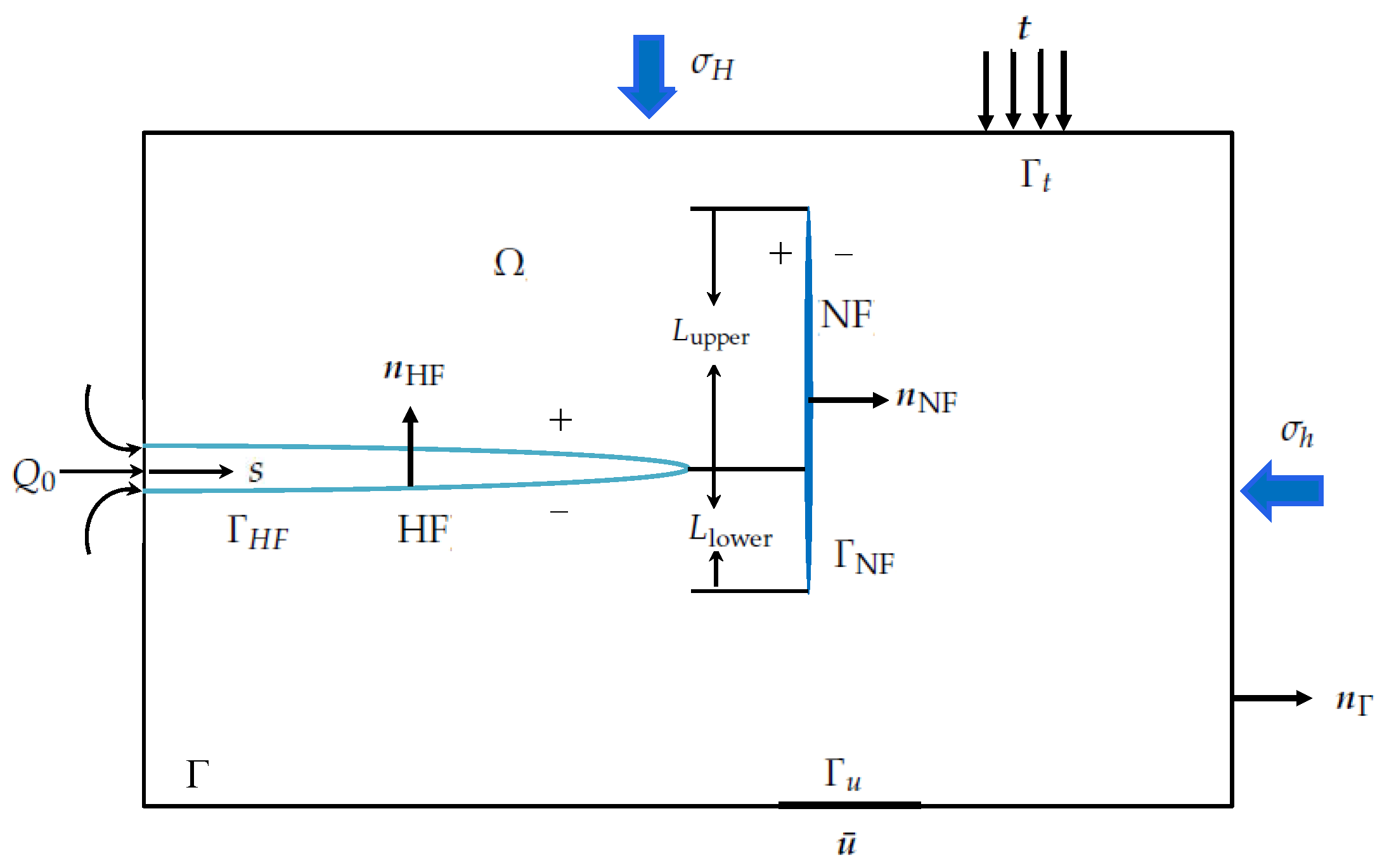
2. Problem Formulation

2.1. Governing Equations of Hydraulic Fracturing Problems

As shown in Figure 1, the domain $\Omega$ denotes a tight reservoir, which includes an HF and an NF. The injection point is located on the middle left of the domain $\Omega$, and the corresponding pump rate is denoted by $Q_0$. As is known, the hydraulic fracturing problem is essentially a fluid–solid interaction process, so its governing equations consist of two parts: the stress equilibrium equation for rock skeleton and fluid pressure equation in the hydraulically driven fracture [52,53,54].

(1) The Stress Equilibrium Equation: According to the theory of elasticity, the stress equilibrium equation is expressed:

$$\nabla ·\mathit{\sigma }+\mathit{b}=\mathbf{0}in\Omega ,$$

(1)

where $\mathit{\sigma }$ denotes the stress tensor; $\mathit{b}$ denotes the body force vector in the rock skeleton. As shown in Figure 1, the boundary conditions are composed of a displacement boundary condition (${\Gamma }_{\mathrm{u}}$) and a force boundary condition (${\Gamma }_{\mathrm{t}}$). They are expressed as

$$\left\{\begin{array}{c}\mathit{u}=\overline{\mathit{u}}on{\Gamma }_{\mathrm{u}},\hfill \\ \mathit{\sigma }·\mathit{n}=\mathit{t},on{\Gamma }_{\mathrm{t}},\hfill \\ \mathit{\sigma }·{\mathit{n}}_{\mathrm{HF}}=p{\mathit{n}}_{\mathrm{HF}},on{\Gamma }_{\mathrm{HF}},\hfill \\ \mathit{\sigma }·{\mathit{n}}_{\mathrm{NF}}={\mathit{t}}_{\mathrm{NF}},on{\Gamma }_{\mathrm{NF}},\hfill \end{array}\right.$$

(2)

where p denotes the fluid pressure on the artificial fracture; ${\mathit{t}}_{\mathrm{NF}}$ denotes the contact traction vector on the NF surface ${\Gamma }_{\mathrm{NF}}$; $\overline{\mathit{u}}$ denotes the displacement imposed on the boundary ${\Gamma }_{\mathrm{u}}$; $\mathit{t}$ denotes the traction vector imposed on the boundary ${\Gamma }_{\mathrm{t}}$.

For brittle rocks, there is a linear relationship between stress tensor and strain tensor under a small deformation assumption, so the corresponding constitutive equation is expressed as

$$\mathit{\sigma }=\mathit{D}:\mathit{\epsilon },$$

(3)

where $\mathit{D}$ denotes the fourth elasticity tensor; $\mathit{\epsilon }$ denotes the strain tensor; the symbol ":" denotes the double dot product of the two tensors.

Under the assumption of small deformation, the relationship between displacement vector $\mathit{u}$ and strain tensor $\mathit{\epsilon }$ are as follows:

$$\mathit{\epsilon }=\frac{1}{2}[\nabla \mathit{u}+{(\nabla \mathit{u})}^T].$$

(4)

(2) Fluid Pressure in an HF: Under lubrication theory assumptions, the velocity profile of the fluid in the HF is that of a planar Poiseuille flow between two parallel plates. Therefore, the fluid pressure in the HF can be expressed as [15,33,34,55,56]

$$\frac{\partial w}{\partial t}-\frac{\partial }{\partial s}\left(k\frac{\partial p}{\partial s}\right)=0,$$

(5)

where w denotes the fracture opening of HF; s denotes the crack propagation direction; t denotes the injection time; k denotes the fracture transmissivity.

According to the cubic law, the fracture transmissivity can be expressed as

$$k=\frac{w^3}{12\mu },$$

(6)

where $\mu$ denotes the viscosity of fracturing fluid.

The corresponding initial and boundary conditions can be expressed as

$$\left\{\begin{array}{c}w(s,0)=0,\hfill \\ w(s_{tip},0)=0,\hfill \\ q(0,t)=Q_0,\hfill \\ q(s_{tip},0)=0,\hfill \end{array}\right.$$

(7)

where $s_{tip}$ denotes the tips of HFs; q denotes the injection rate of fracturing fluid at the crack point s and time t.

It is can be seen that Equation (7) satisfies mathematically the Neumann boundary condition. In order to get a unique solution for the fluid pressure equation, the constraint condition should be additionally imposed. The necessary condition, i.e., the conservation of global mass in the HF can be written as

$${\int }_0^{s_{tip}}wds-{\int }_0^t{Q}_{0}dt=0.$$

(8)

2.2. Crack Propagation Criterion

According to the theory of fracture mechanics, the maximum circumferential stress criterion is adopted to determine the propagation direction of a hydraulically driven fracture at every time t. The artificial fracture will propagate along a direction perpendicular to the maximum circumferential stress. If the stress intensify factor K is no less than the fracture toughness of rock skeleton $K_{\mathrm{IC}}$, the crack will propagate along a certain direction. The interaction integral method in domain form is utilized to calculate the stress intensity factors $K_{\mathrm{I}}$ and $K_{\mathrm{II}}$. The following equation of the interaction integral can be written as [57]

$$I^{(1,2)}={\int }_A[{\sigma }_{ij}^{\left(1\right)}\frac{\partial u_i^2}{\partial x_1}+{\sigma }_{ij}^{\left(2\right)}\frac{\partial u_i^1}{\partial x_1}-W^{(1,2)}{\delta }_{1j}]\frac{\partial q_w}{\partial x_j}dA,$$

(9)

where $I^{(1,2)}$ denotes the interaction integral; $W^{(1,2)}$ denotes the interaction strain energy as follows; $q_w\left(\mathit{x}\right)$ denotes the smooth weighting function, which takes a value from 0 to 1; $\delta$ denotes the Kronecker symbol; the superscripts (1) and (2), respectively, denote the current state and the auxiliary state for the stress and strain field. The corresponding calculation procedures can be described in detail in [40,57,58]

$$W^{(1,2)}={\sigma }_{ij}^{\left(1\right)}{\epsilon }_{ij}^{\left(2\right)}={\sigma }_{ij}^{\left(2\right)}{\epsilon }_{ij}^{\left(1\right)}.$$

(10)

The direction of crack propagation $\theta$ can be computed in a local tip coordinate system:

$$\theta =2\arctan [\frac{1}{4}({\mathrm{K}}_{\mathrm{I}}/{\mathrm{K}}_{\mathrm{II}}+\sqrt{{\mathrm{K}}_{\mathrm{I}}/{\mathrm{K}}_{\mathrm{II}}{)}^2+8})],$$

(11)

where the symbol “arctan” denotes the arc-tangent function.

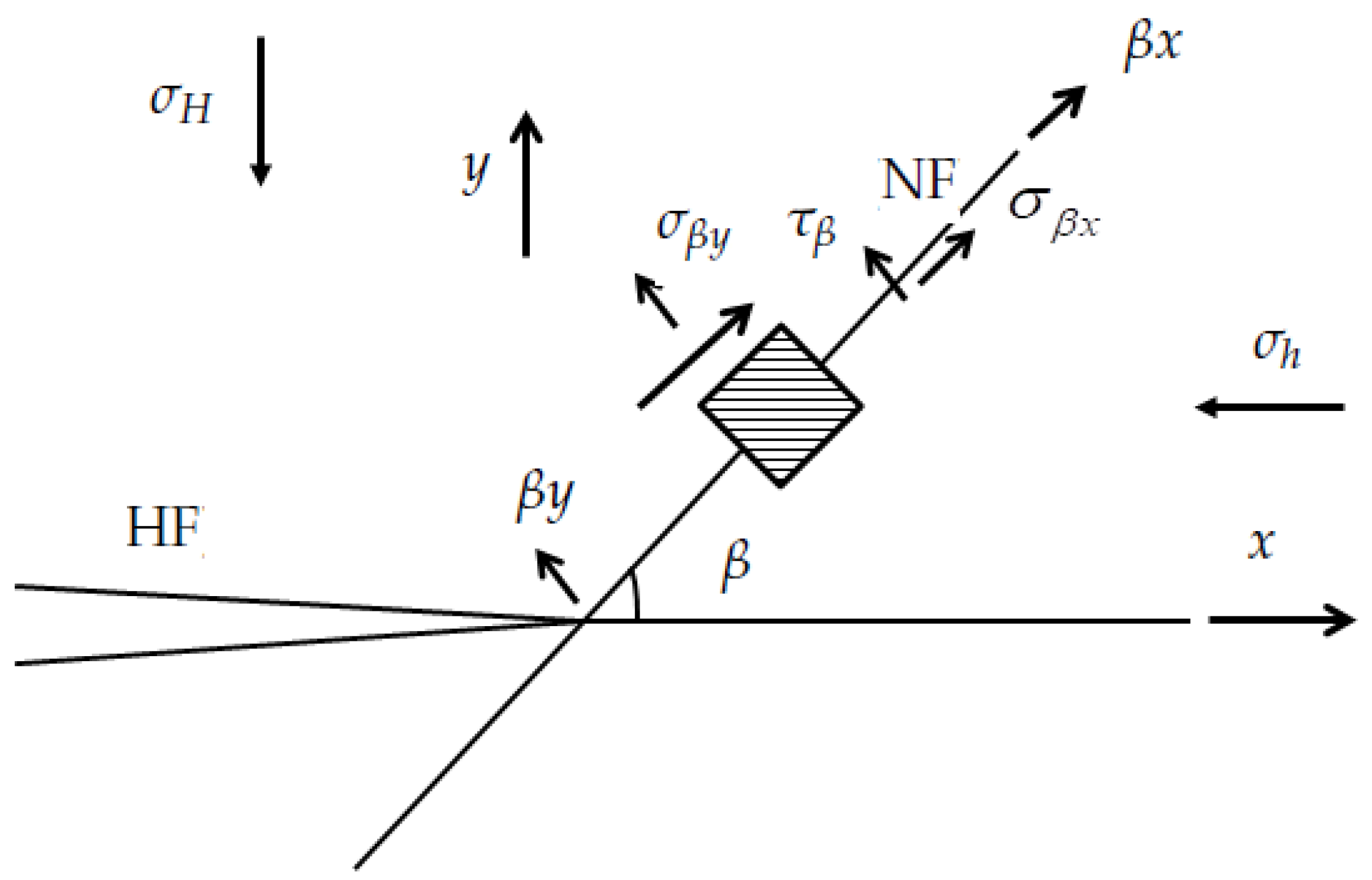
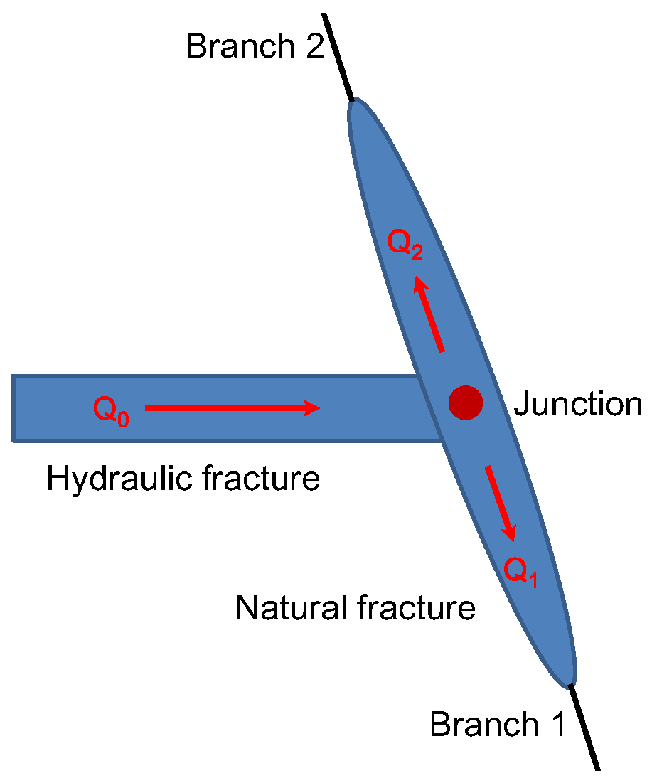
2.3. The Cross Criterion between HF and Frictional NF

As is known, when an HF encounters a frictional NF, there are three possible scenarios: arrested, direction-crossing, or a crossing with an offset [16,23,41]. Here, the extended Renshaw and Pollard rule is adopted to determine the interaction behavior between HF and NF. As shown in Figure 2, if a new fracture initiates on the opposite side of the NF, the maximum principle stress ${\sigma }_1$ will reach the rock tensile stress. Meanwhile, a no-slip condition should be satisfied along the NF surface. Otherwise, the HF will cross directly or branch into NF with an offset. The expressions of the combined shear stress and normal stress are shown in Equation (12), which is described in detail in other references [15,23].

$$\left\{\begin{array}{c}{\sigma }_1=T_0,\hfill \\ {\tau }_{\beta }<S_0-{\mu }_f{\sigma }_{\beta y},\hfill \end{array}\right.$$

(12)

where $\beta$ denotes the intersection angle between HF and NF; ${\tau }_{\beta }$ denotes the combined shear stress on the NF surface under the action of remote stress and the local crack tip stress; ${\sigma }_{\beta y}$ denotes the combined normal stress; $T_0$ denotes the rock tensile strength; $S_0$ denotes the cohesion force of the frictional NF; ${\mu }_f$ denotes the frictional coefficient of the NF surface.

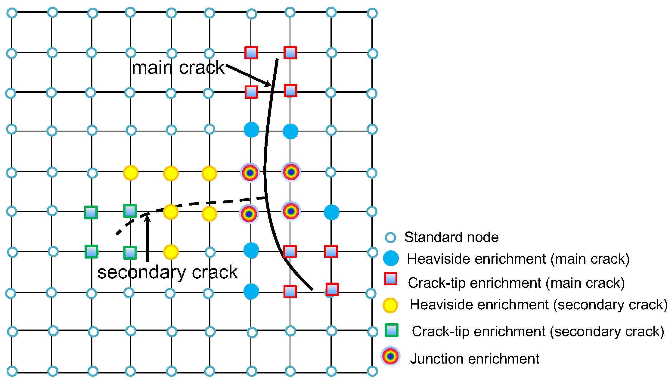
2.4. XFEM and Discretization of the Governing Equations of the Hydraulic Fracturing Problem

The XFEM (extended finite element method) is utilized to approximate the displacement discontinuity on both sides of the HF. In order to represent the multiple cracks, a Junction enrichment function is introduced, as shown in Figure 3. The enriched displacement field can be written as [59].

$$\begin{array}{c}\mathit{u}\left(\mathit{x}\right)=\sum _{I\in N}{N}_I\left(\mathit{x}\right){\mathit{u}}_I+\sum _{j=1}^{M^{dis}}\sum _{J\in N^{dis}}{N}_J\left(\mathit{x}\right)[H\left(\mathit{x}\right)-H\left({\mathit{x}}_J\right)]a_I\hfill \\ +\sum _{k=1}^{M^{tip}}\sum _{K\in N^{tip}}{N}_K\left(\mathit{x}\right)\sum _{\alpha =1}^4[{\Psi }_{tip}^{\alpha }\left(\mathit{x}\right)-{\Psi }_{tip}^{\alpha }\left({\mathit{x}}_K\right)]b_K^{\alpha }\hfill \\ +\sum _{l=1}^{M^{jun}}\sum _{L\in N^{jun}}{N}_L\left(\mathit{x}\right)[J^H\left(\mathit{x}\right)-J^H\left({\mathit{x}}_L\right)]c_L,\hfill \end{array}$$

(13)

where N, $N^{dis}$, $N^{tip}$ and $N^{jun}$, respectively, denote the set of standard nodes, Heaviside enrichment nodes, crack-tip nodes, and junction enrichment nodes; $\mathit{u}$ denotes the standard nodal d.o.f. (degrees of freedom); $a_I$, $b_K^{\alpha }(\alpha =1,4)$, and $c_L$, respectively, denote the corresponding enriched nodal d.o.f.; $M^{dis}$ denotes the number of cracks including the main cracks and the secondary cracks; $M^{tip}$ denotes the number of crack tips; $M^{jun}$ denotes the number of junctions with $M^{jun}=M^{dis}-1$; $H\left(\mathit{x}\right)$ denotes the Heaviside enrichment function; $J^H\left(\mathit{x}\right)$ denotes the junction enrichment function; $\Psi \left(\mathit{x}\right)$ denotes the crack-tip enrichment function; $N_I$, $N_J$, $N_K$, and $N_L$ denote the standard shape function of node I, J, K, and L, respectively.

The Heaviside enrichment function is expressed as [59]

$$H\left(\mathit{x}\right)=\left\{\begin{array}{c}0,if\mathit{x}<0,\hfill \\ 1,if\mathit{x}\ge 0.\hfill \end{array}\right.$$

(14)

The crack-tip enrichment function is defined as

$${\left\{{\Psi }_{tip}^{\alpha }(r,\theta )\right\}}_{\alpha =1}^4=\left\{\sqrt{r}sin\frac{\theta }{2},\sqrt{r}cos\frac{\theta }{2},\sqrt{r}sin\theta sin\frac{\theta }{2},\sqrt{r}sin\theta cos\frac{\theta }{2}\right\},$$

(15)

where ($r,\theta$) denotes the local crack-tip coordinate in the polar coordinate system.

The junction enrichment function $J^H\left(\mathit{x}\right)$ is defined as

$$J^H\left(\mathit{x}\right)=\left\{\begin{array}{c}H\left({\phi }^s\left(\mathit{x}\right)\right),if{\phi }^m\left(\mathit{x}\right)<0,\hfill \\ 0,if{\phi }^m\left(\mathit{x}\right)>0,\hfill \end{array}\right.$$

(16)

where ${\phi }^m\left(\mathit{x}\right)$ and ${\phi }^s\left(\mathit{x}\right)$, respectively, denote the signed distance function of the main crack and the secondary crack. It can be seen that $J^H\left(\mathit{x}\right)$ is equal to 1, $-1$, or 0 on different sub-domains divided by the secondary cracks.

According to the finite element method, the pressure field p and the fracturing opening displacement vector $\mathit{w}$ can be respectively approximated as

$$\mathit{w}=\sum _{I\in S_w}{N}_I^w{\mathit{u}}_I={\mathit{N}}^w\left(s\right)\mathit{U},$$

(17)

$$p\left(s\right)=\sum _{I\in S_{HF}}{N}_I^p{\mathit{p}}_I={\mathit{N}}^p\left(s\right)\mathit{P},$$

(18)

where $\mathit{U}$ and $\mathit{P}$, respectively, denote the global nodal displacement vector and the nodal pressure vector; ${\mathit{N}}^{\mathit{p}}\left(\mathit{s}\right)$ and ${\mathit{N}}^{\mathit{w}}\left(\mathit{s}\right)$, respectively, denote the matrix of the shape function of the fracture opening and pressure.

By substituting the above XFEM formulation, displacement and pressure approximations into the weak form of stress equilibrium equation and lubrication equation, the corresponding discretization forms are written as

$$\mathit{K}\mathit{U}-\mathit{Q}\mathit{P}-{\mathit{F}}^{ext}=\mathbf{0},$$

(19)

$${\mathit{Q}}^T\Delta \mathit{U}+\Delta t\mathit{H}\mathit{P}+\Delta t\mathit{S}=\mathbf{0},$$

(20)

where $\mathit{K}$ denotes the global stiffness matrix; $\mathit{Q}$ denotes the coupling matrix; ${\mathit{F}}^{ext}$ denotes the external loading vector; $\mathit{H}$ denotes the flow matrix; $\Delta t$ denotes the time step; and $\mathit{S}$ denotes the source term. They are, respectively, defined as follows [33,34]:

$$\begin{array}{cc}\mathit{K}\hfill & =\left[\begin{array}{cc}{\int }_{\Omega }{\left({\mathit{B}}^{std}\right)}^T\mathit{D}\left({\mathit{B}}^{std}\right)d\Omega & {\int }_{\Omega }{\left({\mathit{B}}^{std}\right)}^T\mathit{D}\left({\mathit{B}}^{enr}\right)d\Omega \\ {\int }_{\Omega }{\left({\mathit{B}}^{enr}\right)}^T\mathit{D}\left({\mathit{B}}^{std}\right)d\Omega & {\int }_{\Omega }{\left({\mathit{B}}^{enr}\right)}^T\mathit{D}\left({\mathit{B}}^{enr}\right)d\Omega +{\int }_{{\Gamma }_{NF}}{\left({\mathit{N}}^w\right)}^T{\mathit{D}}^{cont}\left({\mathit{N}}^w\right)d\Gamma \end{array}\right]\hfill \\ & =\left[\begin{array}{cc}{\mathit{K}}_{ss}& {\mathit{K}}_{se}\\ {\mathit{K}}_{es}& {\mathit{K}}_{ee}+{\mathit{K}}_{ee}^{cont}\end{array}\right].\hfill \end{array}$$

(21)

In the above Equation (21), ${\mathit{D}}^{cont}$ denotes the contact stiffness matrix of fracture interfaces:

$$\mathit{Q}={\int }_{\Omega }{\left({\mathit{N}}^w\right)}^T{\mathit{n}}_{{\Gamma }_{NF}}\left({\mathit{N}}^p\right)d\Omega ,$$

(22)

$${\mathit{F}}^{ext}={\int }_{{\Gamma }_t}{\left({\mathit{N}}^u\right)}^T\mathit{t}d\Gamma ,$$

(23)

$$\mathit{H}={\int }_{{\Gamma }_{HF}}{{\displaystyle \frac{\partial {\mathit{N}}_p}{\partial s}}}^{T}k{\displaystyle \frac{\partial {\mathit{N}}_p}{\partial s}}ds,$$

(24)

$$\mathit{S}={\mathit{N}}_p{\left(s\right)}^T{\mid }_{s=0}{Q}_0.$$

(25)

As shown in Figure 4, the flow rate in the main crack and secondary crack satisfies the law of conservation, i.e., $Q_0=Q_1+Q_2$, where $Q_1$ and $Q_2$ denote the flow rate in Branches 1 and 2 of the secondary crack, respectively. The nonlinear fluid–solid coupling system of equations of hydraulic fracturing problems can be numerically solved by the Newton–Raphson method. More details are described in [33,34].

3. Results and Discussion

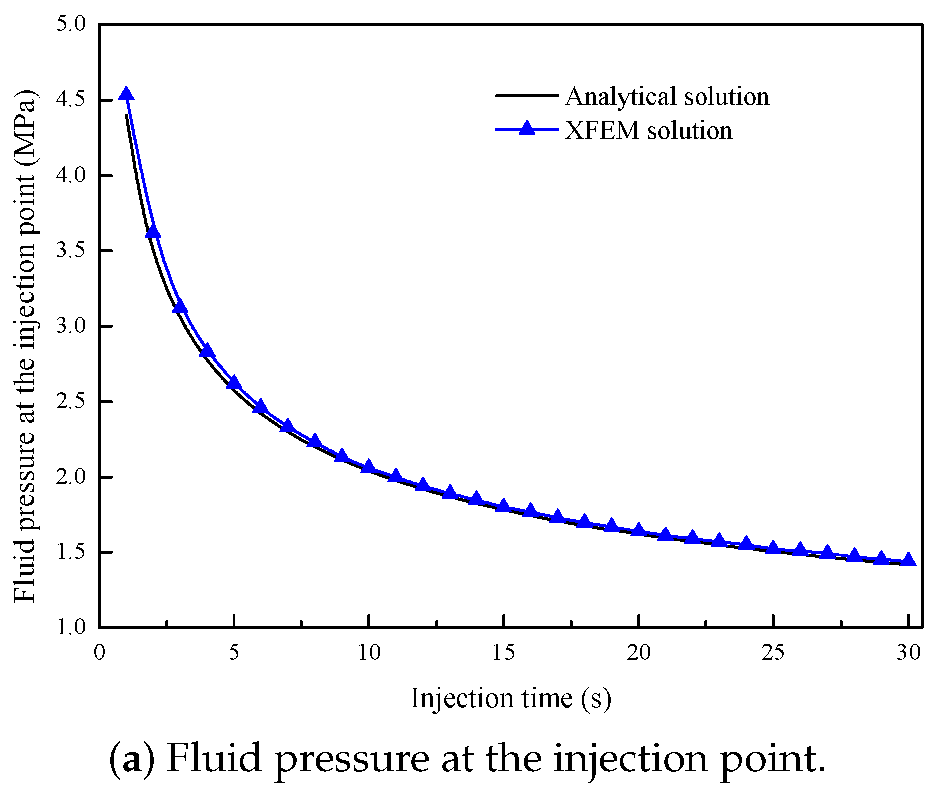
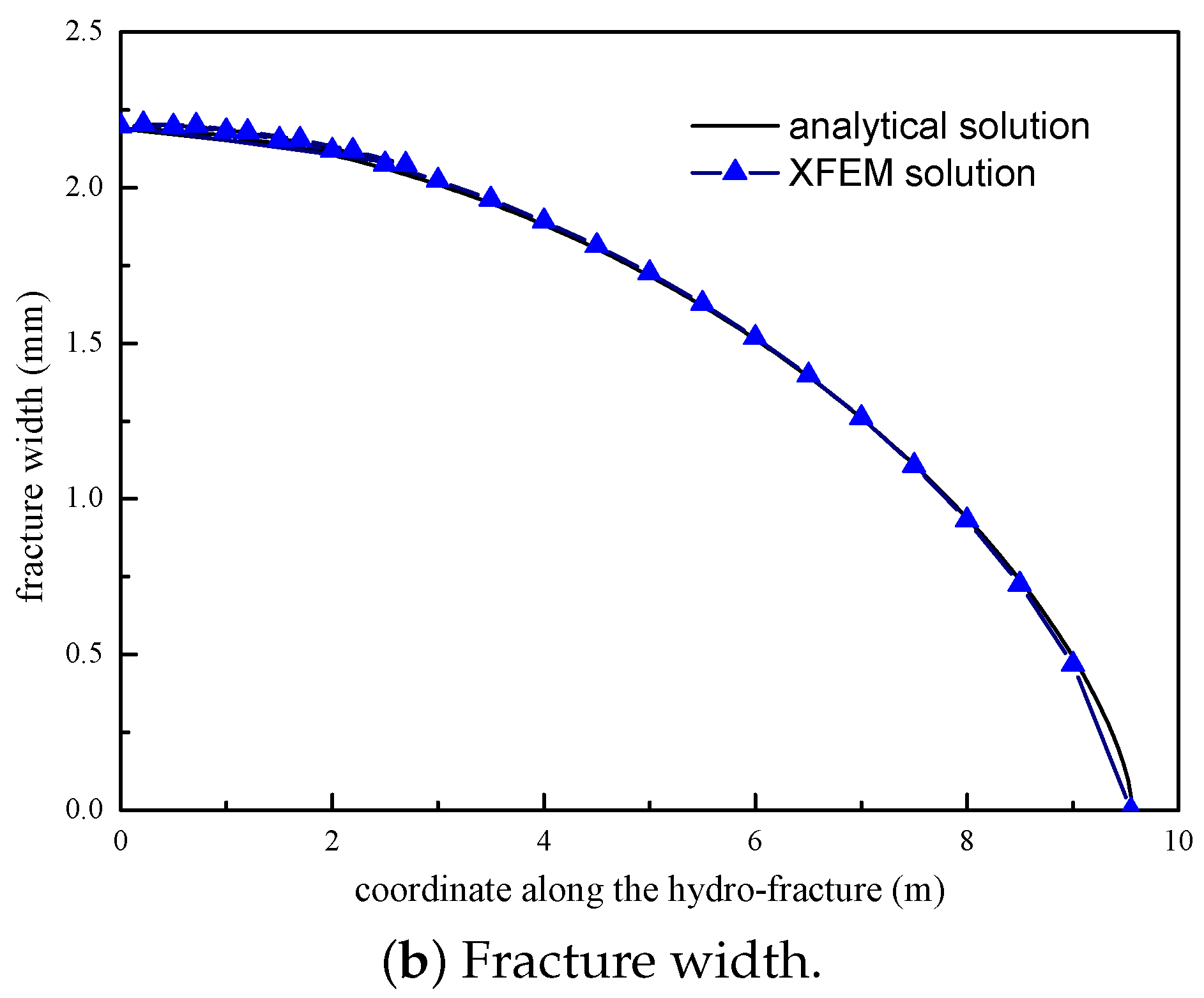
3.1. Verification of the XFEM Model

For the model verification, the results from our models is summarized in Appendix A [33,34]. The verification model of this XFEM code is described in detail in [33,34], so the related process is not repeated in this article. It is shown that the numerical results have good agreement with the experimental results of true tri-axial hydraulic fracturing by TerraTek, Inc. (Salt Lake City, UT, USA). For further details of numerical and experimental procedures and the corresponding results, we refer the reader to References [33,34,60,61].

3.2. Effect of the Location of Natural Fractures on the Diversion of Fracture Network Propagation

In this section, the effect of the location position of an NF on HF propagation paths is determined by numerical simulation using XFEM. The input parameter values of this model are as shown in

Table 1. Input parameter values of the hydro-fracking model.

Input Parameter	Value
Young’s Modulus, E	20 GPa
Poisson’s ratio, $\nu$	0.2
Rock density, $\rho$	2460 $\mathrm{kg}/{\mathrm{m}}^3$
Friction coefficient of NF, ${\mu }_{\mathrm{f}}$	0.3
Cohesion of the NF, $S_0$	0 MPa
Fracture toughness, $K_{\mathrm{IC}}$	1.0 $\mathrm{MPa}·{\mathrm{m}}^{\frac{1}{2}}$
Tensile strength, $T_0$	1.5 MPa
Unconfined compression strength, $\mathrm{UCS}$	100 MPa
Apparent viscosity of fracturing fluid, $\mu$	0.1 $\mathrm{Pa}·\mathrm{s}$
The consistency index of fracturing fluid, K	0.84 $\mathrm{Pa}·{\mathrm{s}}^{\mathrm{n}}$
The flow behavior index of fracturing fluid, n	0.53
Dynamic viscosity index, m	2.0
Fluid pump rate, $Q_0$	0.001 ${\mathrm{m}}^2/\mathrm{s}$
Pore pressure, $P_0$	5 MPa
Maximum horizontal stress, ${\sigma }_{\mathrm{H}}$	5 MPa
Minimum horizontal stress, ${\sigma }_{\mathrm{h}}$	5 MPa

. Under isotropic stress state conditions, the intersection angle between HF and NF is equal to 90°. As shown in Figure 1, the domain is a 25 m × 25 m square, where the injection point is located at the midpoint of the left edge. In this domain, the HF is 2.6 m in length, and the length of NF is equal to 7 m. Based on the above input parameters, the mechanical NF–HF interaction processes in hydraulic fracturing are numerically simulated at different lengths of NF in lower and upper parts, i.e., corresponding to $L_{\mathrm{lower}}$ and $L_{\mathrm{upper}}$ in Figure 1, respectively.

The corresponding crack propagation paths are as shown in Figure 5. It is obvious that fracture diversion occurs near the tips of the NF in all cases. In Figure 5a, when the HF intersects with the NF, the fracturing fluid flows into the opened NF. In the lower parts of the NF, the opened NF firstly propagates along a vertically downward path for a certain length, and it is then diverted along a new direction; in the upper parts of the NF, the opened NF is directly diverted at the upper tip of the original NF. In Figure 5b, both the lower and upper parts of the NF firstly extend vertically downward and upward for a short distance, respectively, and are then diverted to the right-hand side of the graph. However, the length of the lower parts of the diverted fracture (DF) is longer than that of the upper parts of the DF, corresponding to the red line in Figure 1. In Figure 5c, in the upper parts of the NF, the opened fracture can only propagate vertically upward, and cannot be diverted near the tip of the NF; in the lower parts of the NF, the opened fracture can be diverted away from the original NF. By making use of the data in Figure 5, the length of the DF propagation in the upper parts is calculated from the upper tip of the original NF. When the upper length of NF, i.e., $L_{upper}$, is equal to 4, 5, and 6 m, the corresponding length is 3.14, 2.15, and 1.14 m, respectively. If $L_{upper}$ is increased by 2 m, the upper length of the DF will decrease by 2 m. Therefore, it is shown that the longer the upper parts of the original NF are, the more difficult it is for the opened NF to be diverted away from the upper tip of the NF under the conditions of an isotropic stress state, while the lower parts of the original NF is more easily diverted to the right-hand side than the upper parts of the original NF under this circumstance.

The Von-Mises stress distributions are shown in Figure 6, where a blue color represent a relative stress value, while a yellow or red one represent a higher stress value. For all cases of the model, it is shown that there is a small region of stress concentration near the two tips of the original NF, which indicates that a higher pressure is required to divert the opened NF away from the original NF.

The fracture aperture and net pressure curves of the diverted fracture are shown in Figure 7 and Figure 8, respectively. With the decrease of $L_{\mathrm{lower}}$, both curves have revealed an asymmetrical characteristic, which peak at the diverted point in the lower parts. In addition, at the intersection point between HF and NF, their corresponding values take second place. The fracture aperture and net pressure in the lower parts of the DF are much greater than those in the upper parts. By comparison, in the case of $L_{\mathrm{lower}}=3\mathrm{m}$ and $L_{\mathrm{lower}}=4\mathrm{m}$, their curves are nearly symmetrical. This indicates that, under the combined action of remote stress and local crack-tip stress, the variation tendency of the fracture aperture and the net pressure is quite different from that in the case of only a single HF.

The flow rate in the diverted fracture is shown in Figure 9. When fluid flows into the intersection point between HF and NF, it will flow upward and downward, respectively. If the value of the flow rate is negative, fluid will flow upward; otherwise, it will flow downward. It is shown that the flow rate in the lower parts of the DF is much greater than that in the upper parts. Therefore, the fracture aperture and net pressure in the lower parts of the DF is greater than that in the upper parts under the condition of the same fluid viscosity. With the decrease of $L_{\mathrm{lower}}$, fluid flows downward more easily. Thus, the lower parts of the original NF is more easily diverted than the upper parts of the original NF. This may explain the results in Figure 5.

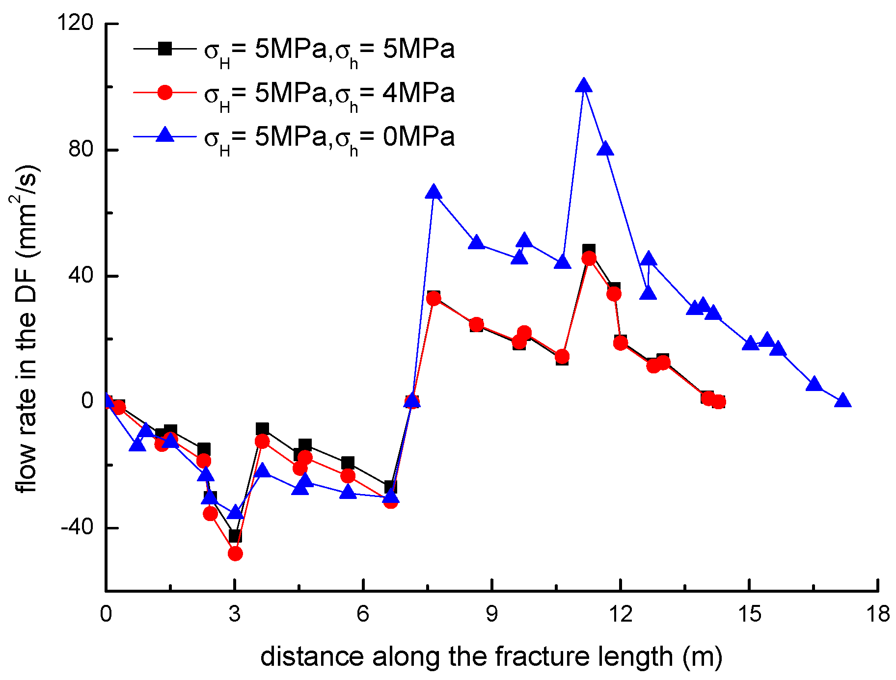
3.3. Effect of Horizontal Stress Differences on the Diversion of Fracture Network Propagation

Based on input parameters in Table 1, the effect of the remote stress difference on the diversion of fracture network propagation is numerically simulated at different levels of minimum horizontal stresses ${\sigma }_{\mathrm{h}}$: 5, 4, and 0 MPa; the maximum horizontal stress ${\sigma }_{\mathrm{H}}$ is kept constant (5 MPa) in all cases of this model. At the same time, $L_{\mathrm{lower}}$ = 3 m, $L_{\mathrm{upper}}$ = 4 m, and the NF–HF intersection angle is equal to 90°.

The corresponding crack propagation paths are shown in Figure 10, in which the deflection angle is defined the angle between NF and DF at the tips of the original NF. According to the data in Figure 10, the deflection angle in the upper parts is calculated. When the horizontal stress difference is, respectively, equal to 0 and 5 MPa, the corresponding deflection angle is 59.2° and 90°, respectively. If the stress difference is increased by 5 MPa, the deflection angle in the upper parts is increased by 30.8°. The higher the horizontal stress difference is, the greater the deflection angle is. In Figure 10c, i.e., $\Delta \sigma$ = 5 MPa, the opened NF firstly diverts and propagates along the direction of minimum horizontal stress and finally tends to extend along the preferred fracture plane (PFP) direction in petroleum engineering. By contrast, when the stress state is approximately isotropic, crack propagation in both the lower and upper parts will extend along the minimum horizontal stress direction for some length. This indicates that crack propagation of the opened NF is a complex mechanical process under the combined action of the local crack-tip and the remote stress state.

As shown in Figure 11c, there is a lower Von-Mises stress region (corresponding to blue area on the contour) located on the right of DF for 5 MPa stress difference. This propagates the diverted fracture along the PFP. In Figure 11a,b, both cases correspond to a lower stress difference, and the lower stress region is mainly near the two crack tips. The local stress distribution is an explanation to interpret crack paths in Figure 10.

The fracture aperture and net pressure curves of DF are shown in Figure 12 and Figure 13, respectively. The fracture aperture curve reveals an asymmetrical characteristic, while the net pressure curve reveals a nearly symmetrical characteristic. The fracture aperture peaks at a global maximum value at the inflection point, where the opened fracture in the upper parts diverts to the right side in Figure 10; at the NF–HF intersection point, the fracture aperture takes the second place; at the inflection point in the lower parts, it takes the third place. The net pressure reaches a maximum at the intersection point, and there are two inflection points on this curve. This means that the opened fracture diverts to the right side. The higher the stress difference is, the greater the net pressure it requires, which leads to a greater fracture aperture.

The flow rate in the DF is shown in Figure 14. It is obvious that the flow rate in the upper parts is much greater than that in the lower parts. Therefore, the fracture aperture and net pressure in the upper parts are greater than those in the lower parts for the same fluid viscosity. This might explain the results of fracture aperture and net pressure in Figure 12 and Figure 13.

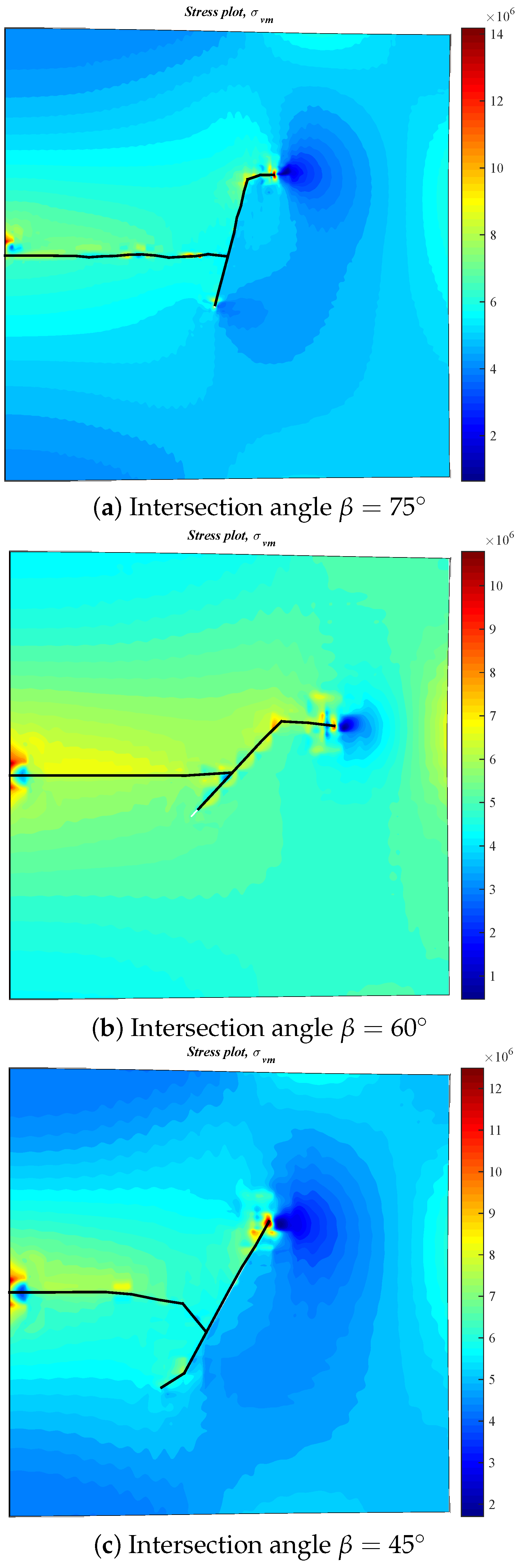
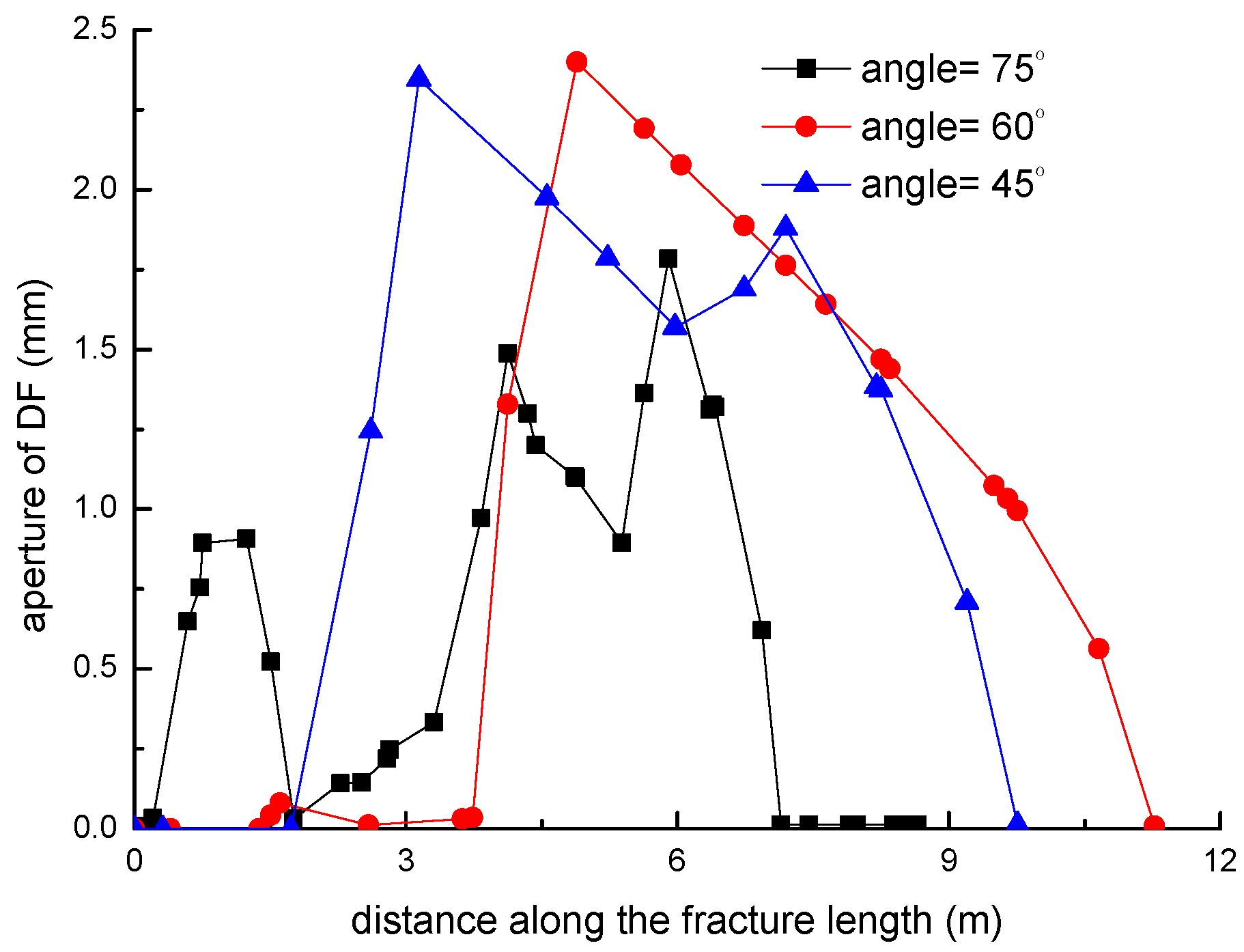
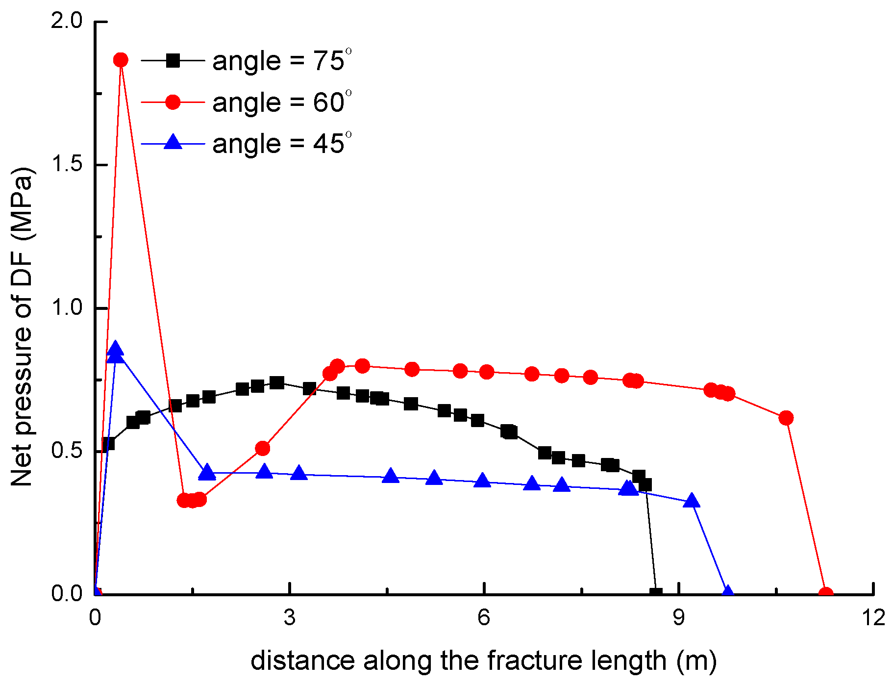
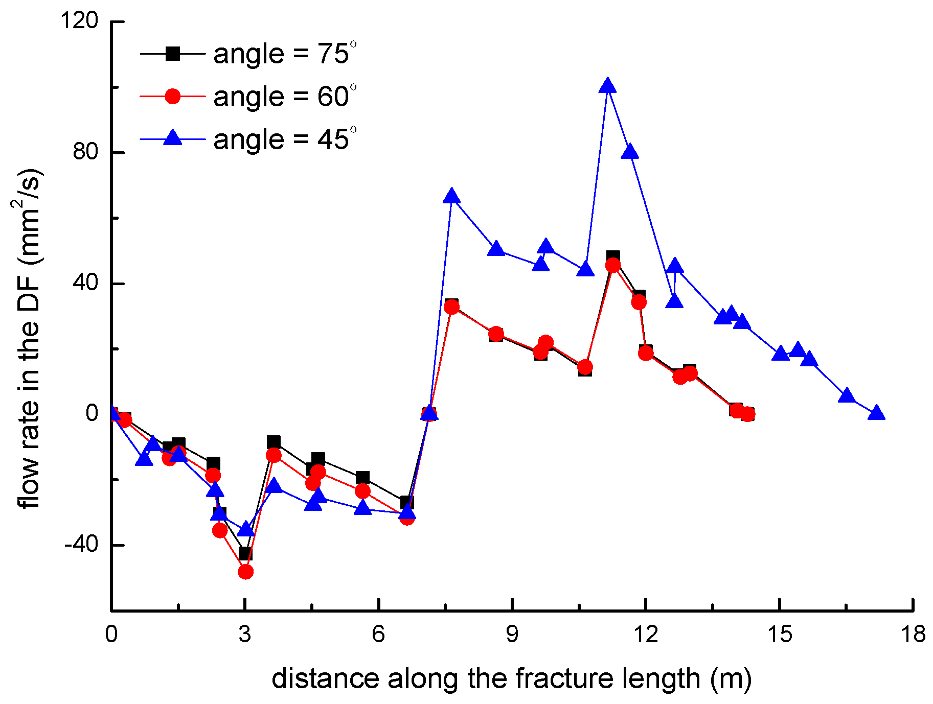
3.4. Effect of the NF–HF Intersection Angle on the Diversion of Fracture Network Propagation

Based on the input parameters in Table 1, the effect of the NF–HF intersection angle on the diversion of fracture network propagation is numerically simulated at different levels of intersection angles $\beta$: 75°, 60°, and 45°; both the maximum and minimum horizontal principle stresses are equal to 5 MPa in all cases of this model. Meanwhile, $L_{\mathrm{lower}}$ and $L_{\mathrm{upper}}$ are, respectively, 3 m and 4 m.

The corresponding crack propagation paths are as shown in Figure 15. Under the condition of isotropic stress state, the NF–HF intersection angle will have a significant impact on the propagation direction of the primary HF, i.e., the black dotted line in Figure 15, when HF is approaching NF. With the decrease of the intersection angle, the primary HF deflects from the horizontal line. When the NF–HF intersection angle is greater than 60° (in Figure 15a,b), the opened NF in the upper parts is more easily diverted away from the original NF than that in the lower parts under the combined action of remote stress and the crack-tip stress field. However, the intersection angle is less than 60° (in Figure 15c). The opened NF in the lower parts is more easily diverted away from the original NF than that in the upper parts under the combined action of remote stress and the crack-tip stress field. By making use of the data in Figure 15, the deflection angle for the primary HF was calculated. When the intersection angle is decreased from 75° to 45°, the corresponding deflection angle is increased from 0° to 61.2°. This indicates that the NF–HF intersection angle will have a significant impact on the diversion propagation of the primary HF and the secondary opened NFs.

The Von-Mises stress distributions at different levels of NF–HF intersection angle are shown in Figure 16. In Figure 16a, there is a stress concentration region near the diversion point in the upper parts of the NF, which indicates that it will require a high net pressure to divert the opened fracture upward. In Figure 16b, the Von-Mises stress in the upper parts is greater than that in the lower parts, which causes the subsequent fracture to easily divert upward. In Figure 16c, the Von-Mises stress on the left of the NF is greater than that on the right, so it is more easily diverted downward.

The fracture aperture and net pressure curves of the DF are shown in Figure 17 and Figure 18, respectively. In the case of $\beta =75$°, the fracture aperture and net pressure in the upper parts is greater than that in the lower parts. In particular, the fracture aperture and net pressure near the diversion point in the lower parts is close to zero, and this is consistent with the results of Von-Mises stress at this point. In the other two cases, the maximum values of the fracture aperture and the net pressure are at the diversion point in the lower parts. The smaller the intersection angle is, the greater the net pressure it requires to divert the fracture.

The flow rate in DF is shown in Figure 19. It is obvious that, in the case of $\beta =45$°, the flow rate in the upper parts is much greater than that in the lower parts. This indicates that it is easy for fracturing fluid to flow upward when the intersection angle is small. This is a possible reason for explaining the results in Figure 17 and Figure 18.

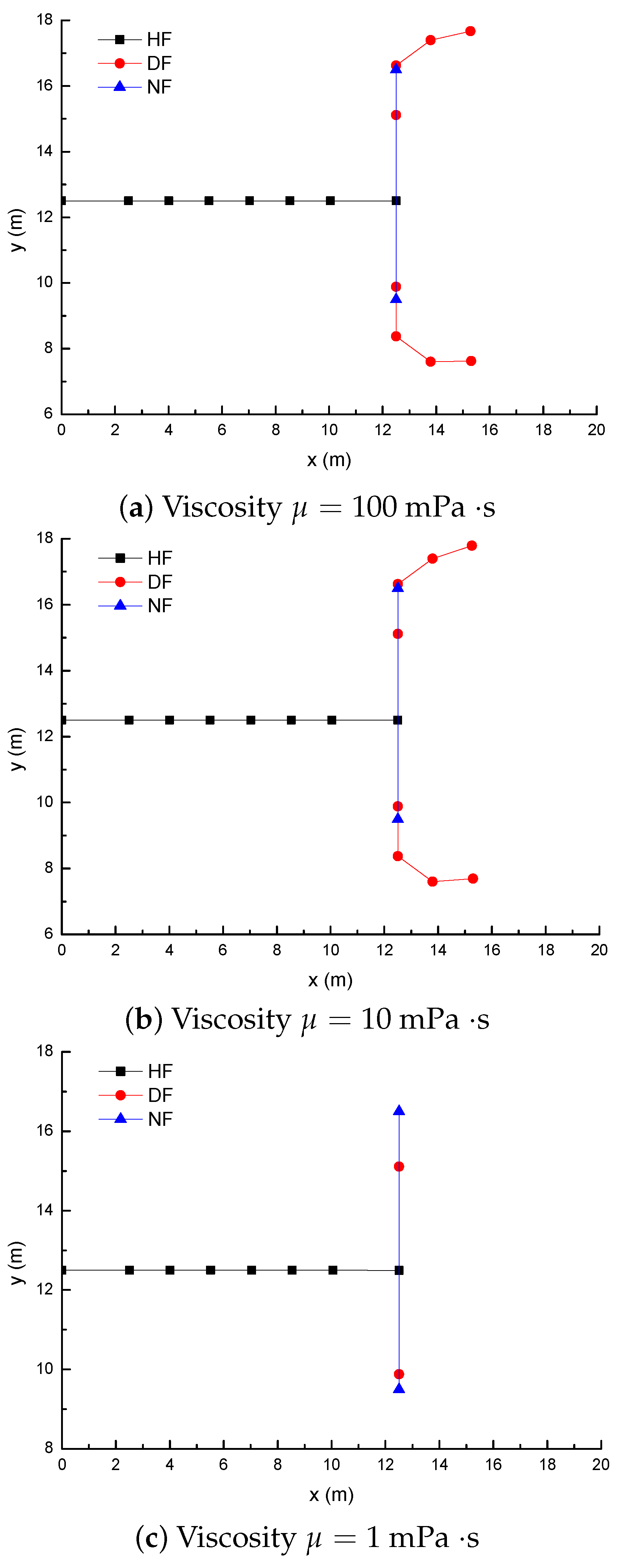
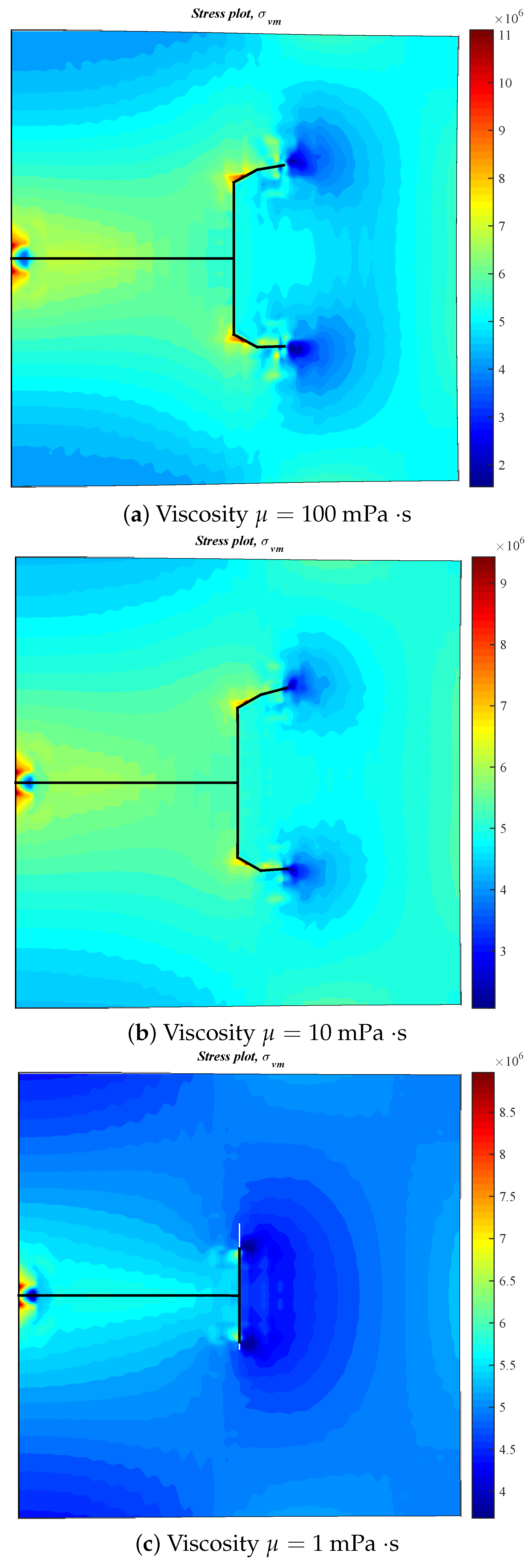
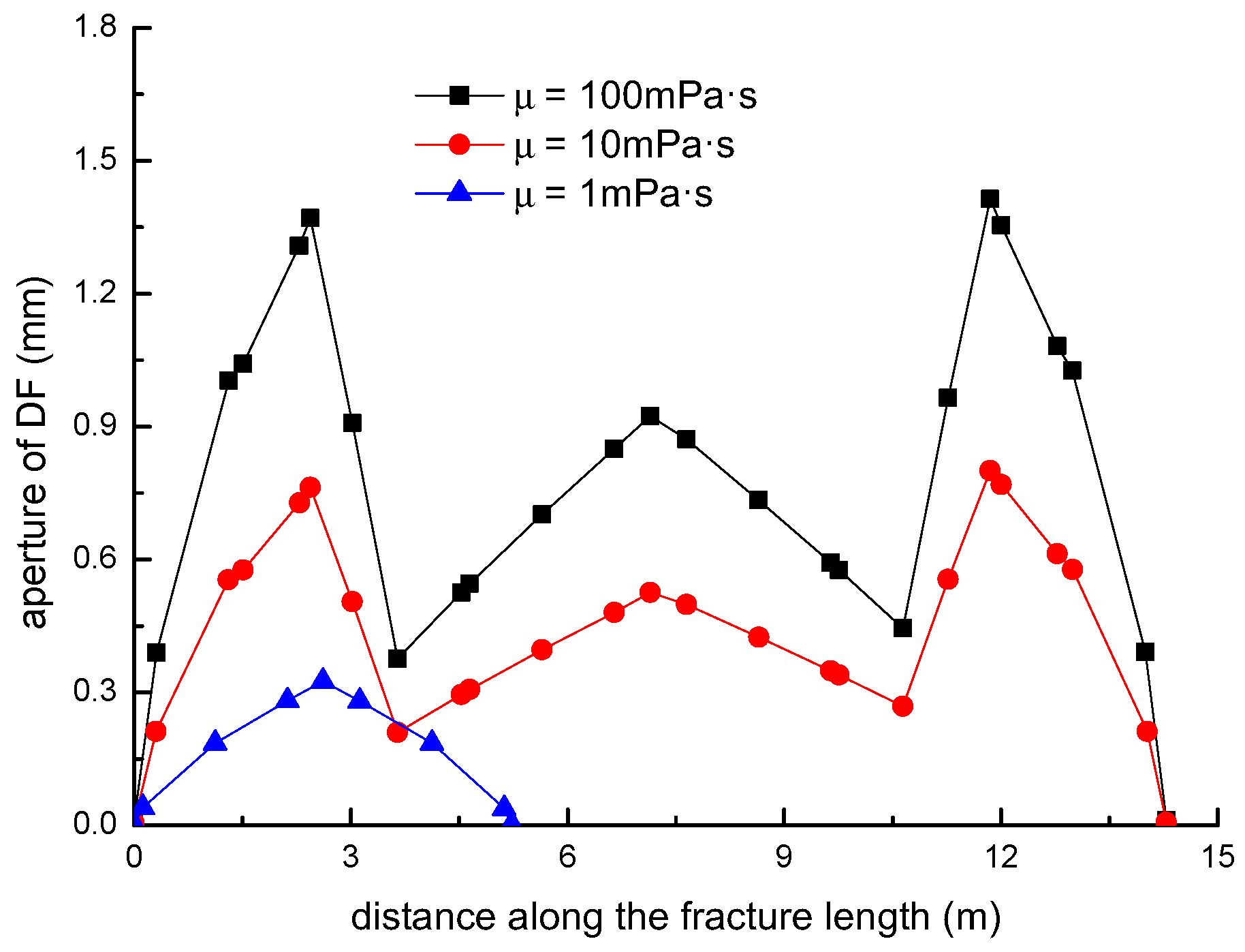
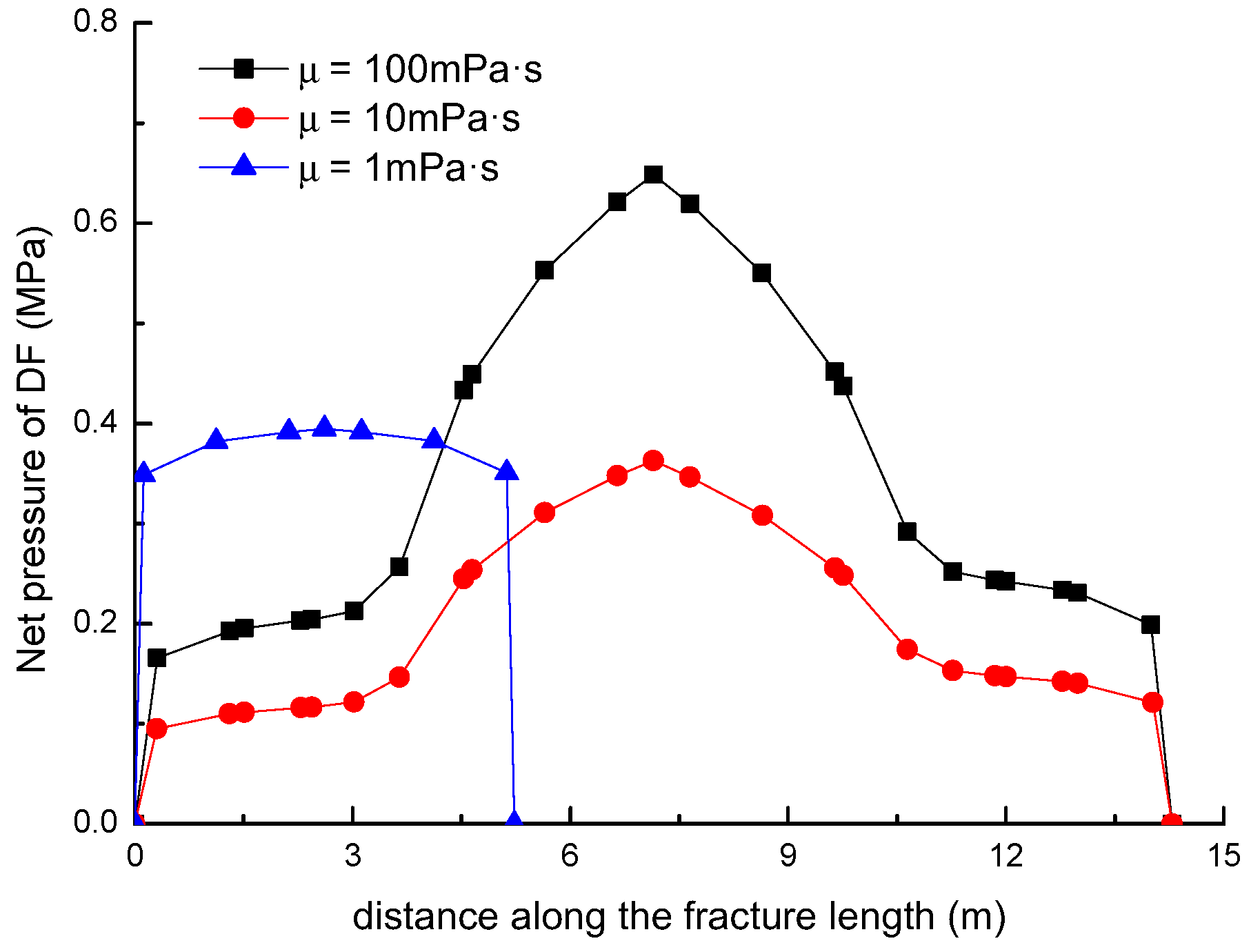
3.5. Effect of Fluid Viscosity on the Diversion of Fracture Network Propagation

Based on the input parameters in Table 1, the effect of the viscosity of fracturing fluid on the diversion of fracture network propagation is numerically simulated at different levels of viscosity $\mu$: 100 mPa$·$s, 10 mPa$·$s, and 1 mPa$·$s [62]. In this model, the maximum and minimum horizontal stresses are kept constant (5 MPa) for all cases. Meanwhile, the NF–HF intersection angle is equal to 90.

The corresponding crack propagation paths are shown in Figure 20. By making use of the data in Figure 20, the length of DF is calculated. When the fluid viscosity is increased from 100 mPa$·$s to 1 mPa$·$s, the length of DF is increased from 14.29 to 5.23 m. It is clear that the smaller the viscosity is, the more difficult the opened fracture diverts into a new direction. When the viscosity is equal to 1 mPa$·$s, artificial fracture will propagate along the NF direction under given conditions. This indicates that more energy is required to divert the opened NF upward and downward.

The Von-Mises stress distributions at different levels of fluid viscosity are shown in Figure 21. In Figure 21c, there is a lower Von-Mises stress area on the right of the NF, which makes the opened NF propagate along the original NF direction. This is consistent with the results in Figure 20.

The fracture aperture and net pressure curves of the DF are shown in Figure 22 and Figure 23, respectively. They are close to symmetrical about the axis of the original HF under the condition of an isotropic stress state. In the cases of $\mu =100$ mPa $·$s and $\mu =10$ mPa $·$s, there are two inflection points on the curves, which correspond to the diversion point in the lower and upper parts of the NF. The greater the fluid viscosity is, the greater the fracture aperture and net pressure are.

The flow rate in the DF is as shown in Figure 24. Obviously, the greater the viscosity is, the greater the flow rate is, and thus the easier it is for the secondary fracture to divert. This might explain the results in Figure 20 and Figure 21 [63].

4. Conclusions

This paper investigates the diversion mechanisms of a fracture network in tight formations with frictional NFs by means of the XFEM technique. The effects of some key factors such as the location of the NF, the intersection angle between the NF and HF, the horizontal stress difference, and the fluid viscosity on the mechanical diversion behavior of the HF were analyzed in detail. The following main conclusions can be drawn:

(1)

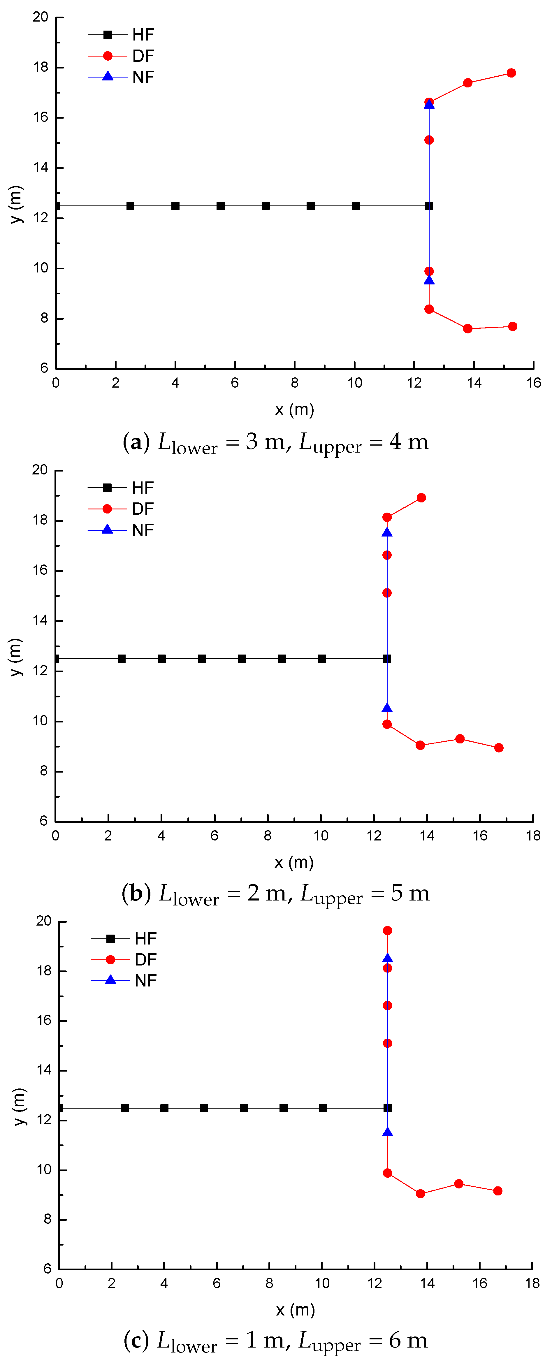
Fracture diversion propagation will occur near the two tips of the opened NF after an HF is intersecting with an NF. The numerical results show that some key factors such as the NF position, the NF–HF intersection angle, the horizontal stress differences, and the fluid viscosity have a significant impact on the diversion propagation in the upper and lower parts of the opened NF.

(2)

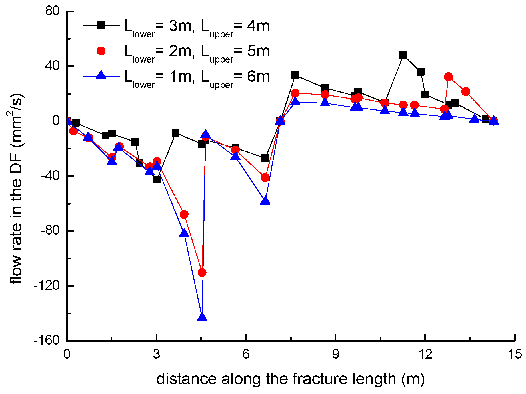
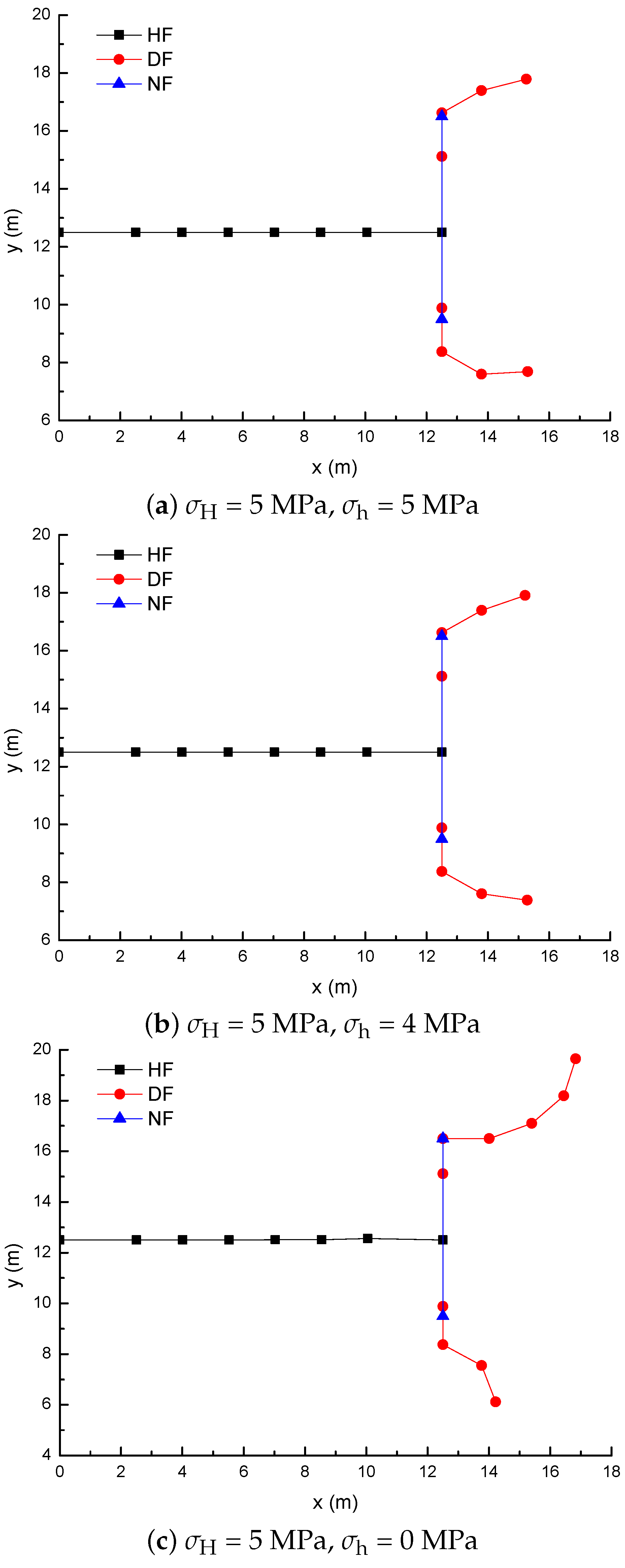
For a constant length of NF (7 m), the upper length of the DF decreases by about 2 m with a 2 m increment of the upper length of the NF ($L_{upper}$), while the length of the DF increases 9.06 m, with the fluid viscosity increased from 1 to 100 mPa.s; (2) the deflection angle in the upper parts increases by 30.8° with the stress difference increased by 5 MPa, while the deflection angle increases by 61.2° with the intersection angle decreased from 75° to 45°.

(3)

The longer the upper parts of the original NF are, the more difficult it is for the opened NF to divert away from the upper tip of the NF under the conditions of an isotropic stress state, while the lower parts of the original NF is more easily diverted to the right-hand side than the upper parts of the original NF. The NF–HF intersection angle will have a significant impact on the diversion propagation of the primary HF and the secondary opened NFs.

(4)

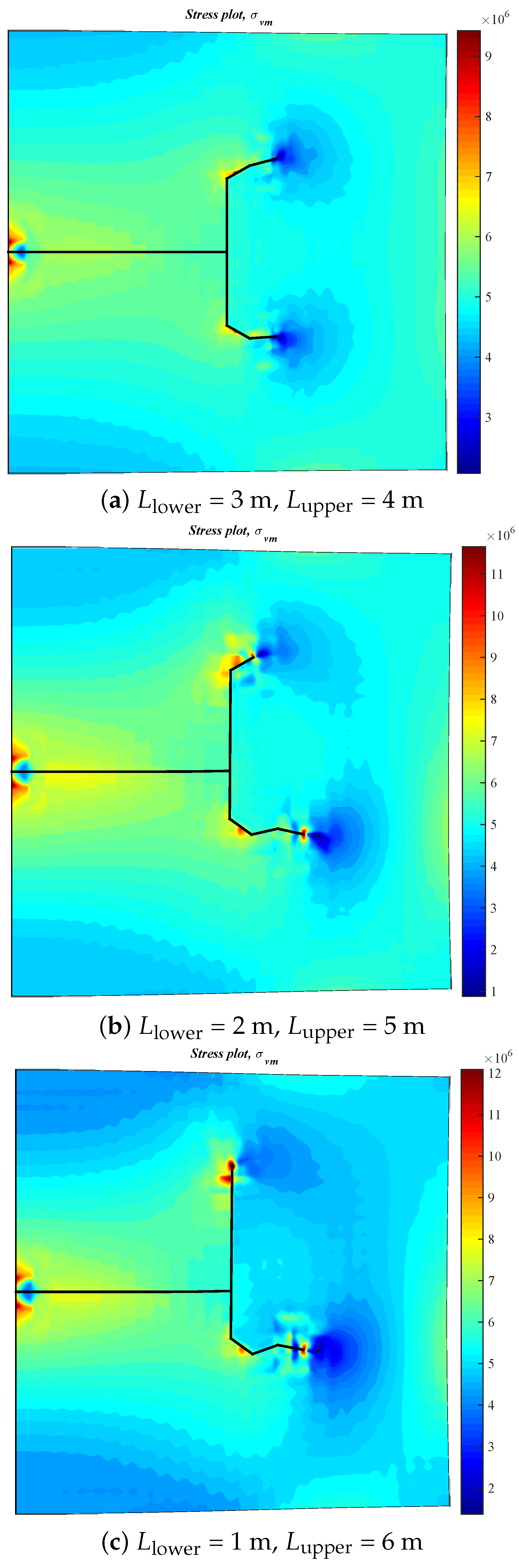
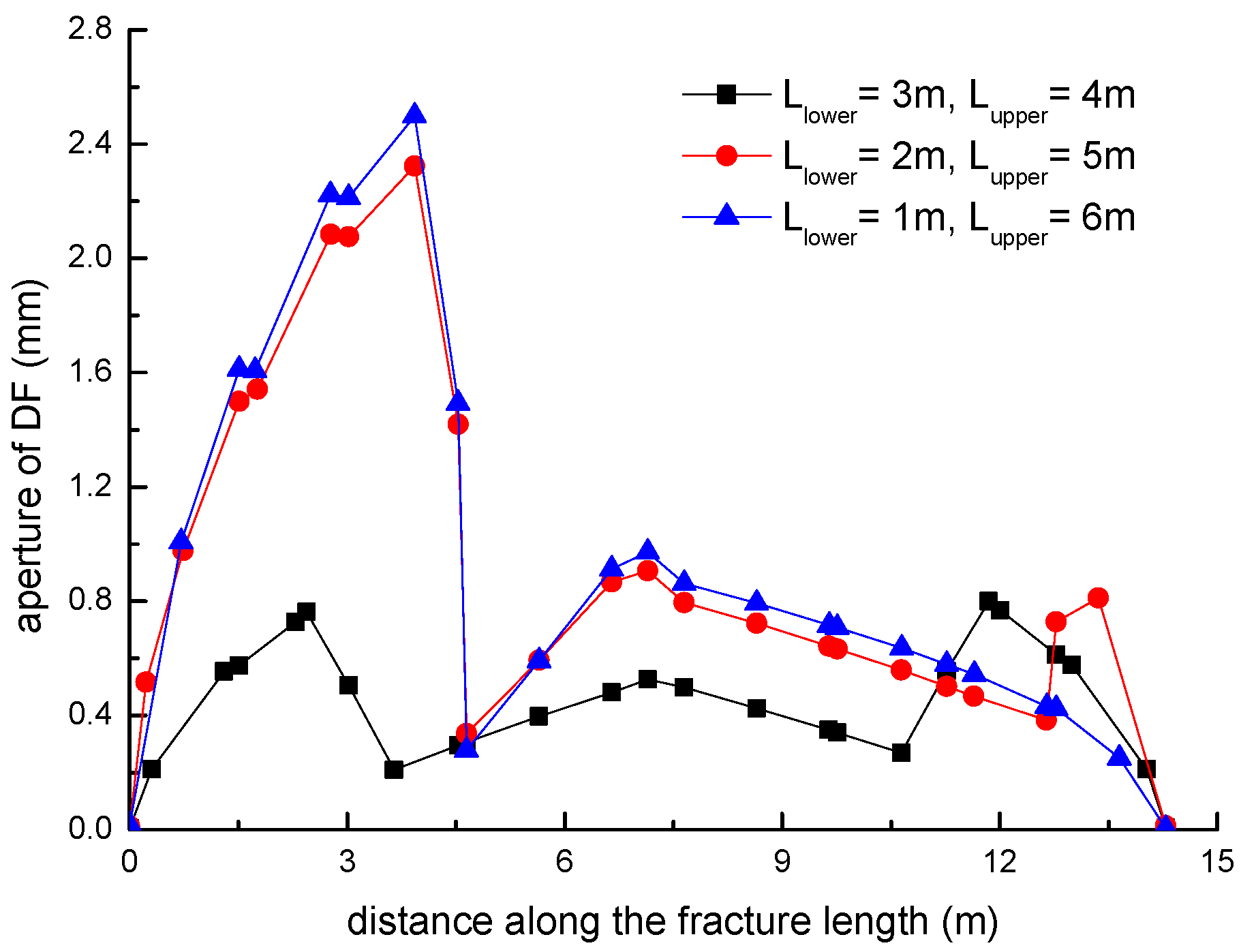
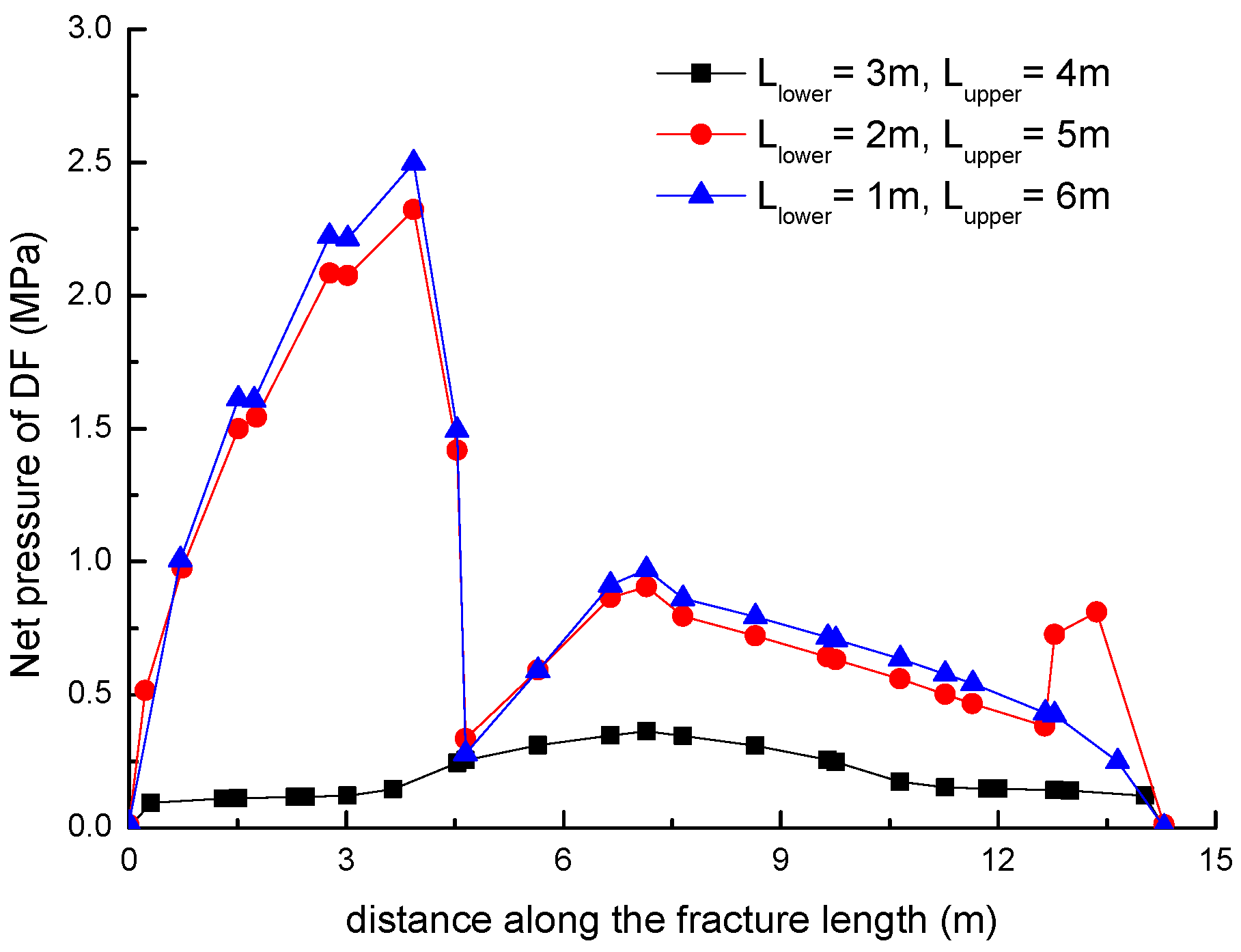
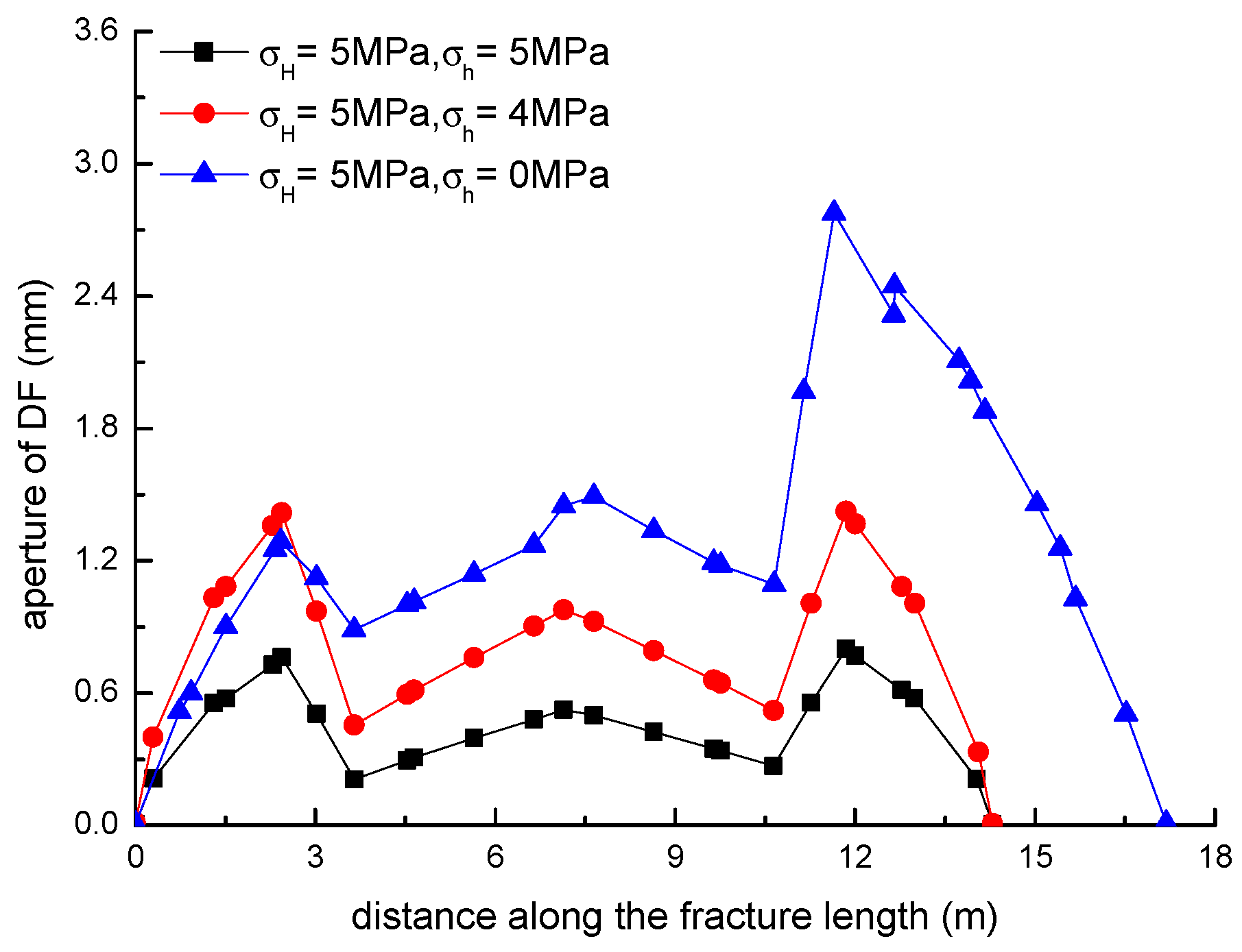
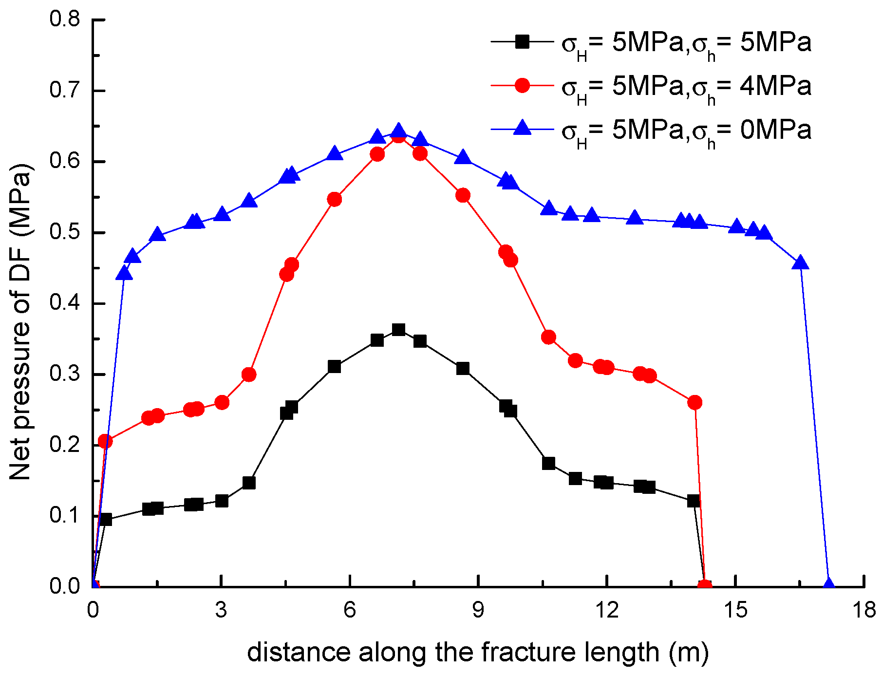
In general, the distributions of fracture aperture, net pressure, and flow rate reveal asymmetrical characteristics for the secondary hydraulically driven fractures. For the distribution of Von-Mises stress, there is usually a concentrated stress zone area near the turning point of the secondary cracks, which corresponds to the inflection points on the curves of the fracture aperture and net pressure.

(5)

The diversion mechanisms of the fracture network are the results of the combined action of all factors. This will provide a new perspective on the mechanisms of fracture network generation. Future work should determine the primary and secondary relations of various factors by means of experiments and numerical calculation.

References

1. Pang, Y.; Soliman, M.Y.; Deng, H.; Emadi, H. Analysis of effective porosity and effective permeability in shale-gas reservoirs with consideration of gas adsorption and stress effects. SPE J. 2017, 22, 1739–1759. [Google Scholar] [CrossRef]
2. Shen, Y.; Ge, H.; Li, C.; Yang, X.; Ren, K.; Yang, Z.; Su, S. Water imbibition of shale and its potential influence on shale gas recovery—A comparative study of marine and continental shale formations. J. Nat. Gas Sci. Eng. 2016, 35, 1121–1128. [Google Scholar] [CrossRef]
3. Pang, Y.; Soliman, M.; Deng, H.; Emadi, H. Effect of methane adsorption on stress-dependent porosity and permeability in shale gas reservoirs. In Proceedings of the SPE Low Perm Symposium, Denver, CO, USA, 5–6 May 2016. [Google Scholar]
4. Matsunaga, I.; Kobayashi, H.; Sasaki, S.; Ishida, T. Studying hydraulic fracturing mechanism by laboratory experiments with acoustic emission monitoring. In Proceedings of the 34th U.S. Symposium on Rock Mechanics (USRMS), Madison, WI, USA, 28–30 June 1993. [Google Scholar]
5. Wang, W.; Su, Y.; Sheng, G.; Cossio, M.; Shang, Y. A mathematical model considering complex fractures and fractal flow for pressure transient analysis of fractured horizontal wells in unconventional oil reservoirs. J. Nat. Gas Sci. Eng. 2015, 23, 139–147. [Google Scholar] [CrossRef]
6. Zhang, J.; Ouyang, L.; Zhu, D.; Hill, A. Experimental and numerical studies of reduced fracture conductivity due to proppant embedment in the shale reservoir. J. Pet. Sci. Eng. 2015, 130, 37–45. [Google Scholar] [CrossRef] [Green Version]
7. Wang, W.; Shahvali, M.; Su, Y. Analytical solutions for a quad-Linear flow model derived for multistage fractured horizontal wells in tight oil reservoirs. J. Energy Resour. Technol. 2017, 139, 012905. [Google Scholar] [CrossRef]
8. Wang, W.; Shahvali, M.; Su, Y. A semi-analytical model for production from tight oil reservoirs with hydraulically fractured horizontal wells. Fuel 2015, 158, 612–618. [Google Scholar] [CrossRef]
9. Cai, J.; Wei, W.; Liu, R.; Wang, J. Fractal characterization of dynamic fracture network extension in porous media. Fractals 2017, 25, 1750023. [Google Scholar] [CrossRef]
10. Wang, F.; Yang, K.; Cai, J. Fractal characterization of tight oil reservoir pore structure using nuclear magnetic resonance and mercury intrusion porosimetry. Fractals 2018, 26, 1840017. [Google Scholar] [CrossRef]
11. Singh, H.; Cai, J. Screening improved recovery methods in tight-oil formations by injecting and producing through fractures. Int. J. Heat Mass Transf. 2018, 116, 977–993. [Google Scholar] [CrossRef]
12. Detournay, E.; Cheng, A.D.; Roegiers, J.C.; McLennan, J. Poroelasticity considerations in In Situ stress determination by hydraulic fracturing. Int. J. Rock Mech. Min. Sci. Geomech. Abstr. 1989, 26, 507–513. [Google Scholar] [CrossRef]
13. Schmitt, D.; Zoback, M. Poroelastic effects in the determination of the maximum horizontal principal stress in hydraulic fracturing tests—A proposed breakdown equation employing a modified effective stress relation for tensile failure. Int. J. Rock Mech. Min. Sci. Geomech. Abstr. 1989, 26, 499–506. [Google Scholar] [CrossRef]
14. Mahrer, K.D. A review and perspective on far-field hydraulic fracture geometry studies. J. Pet. Sci. Eng. 1999, 24, 13–28. [Google Scholar] [CrossRef]
15. Yew, C.H.; Weng, X. Mechanics of Hydraulic Fracturing, 2nd ed.; Gulf Professional Publishing: Houston, TX, USA, 2014. [Google Scholar]
16. Hossain, M.M.; Rahman, M. Numerical simulation of complex fracture growth during tight reservoir stimulation by hydraulic fracturing. J. Pet. Sci. Eng. 2008, 60, 86–104. [Google Scholar] [CrossRef]
17. Yuan, B.; Zheng, D.; Moghanloo, R.G.; Wang, K. A novel integrated workflow for evaluation, optimization, and production predication in shale plays. Int. J. Coal Geol. 2017, 180, 18–28. [Google Scholar] [CrossRef]
18. Yuan, B.; Su, Y.; Moghanloo, R.G.; Rui, Z.; Wang, W.; Shang, Y. A new analytical multi-linear solution for gas flow toward fractured horizontal wells with different fracture intensity. J. Nat. Gas Sci. Eng. 2015, 23, 227–238. [Google Scholar] [CrossRef]
19. Wu, K.; Chen, Z.; Li, X.; Guo, C.; Wei, M. A model for multiple transport mechanisms through nanopores of shale gas reservoirs with real gas effect–adsorption-mechanic coupling. Int. J. Heat Mass Transf. 2016, 93, 408–426. [Google Scholar] [CrossRef]
20. Wei, B.; Li, Q.; Jin, F.; Wang, C. The potential of a novel nanofluid in enhancing oil recovery. Energy Fuels 2016, 30, 2882–2891. [Google Scholar] [CrossRef]
21. Zhang, Q.; Su, Y.; Wang, W.; Lu, M.; Sheng, G. Gas transport behaviors in shale nanopores based on multiple mechanisms and macroscale modeling. Int. J. Heat Mass Transf. 2018, 125, 845–857. [Google Scholar] [CrossRef]
22. Renshaw, C.; Pollard, D. An experimentally verified criterion for propagation across unbounded frictional interfaces in brittle, linear elastic materials. Int. J. Rock Mech. Min. Sci. Geomech. Abstr. 1995, 32, 237–249. [Google Scholar] [CrossRef]
23. Gu, H.; Weng, X. Criterion for fractures crossing frictional interfaces at non-orthogonal angles. In Proceedings of the 44th U.S. Rock Mechanics Symposium and 5th U.S.-Canada Rock Mechanics Symposium, Salt Lake City, UT, USA, 27–30 June 2010. [Google Scholar]
24. Chen, Z.; Jeffrey, R.G.; Zhang, X.; Kear, J. Finite-element simulation of a hydraulic fracture interacting with a natural fracture. SPE J. 2017, 22, 219–234. [Google Scholar] [CrossRef]
25. Zou, Y.; Zhang, S.; Ma, X.; Zhou, T.; Zeng, B. Numerical investigation of hydraulic fracture network propagation in naturally fractured shale formations. J. Struct. Geol. 2016, 84, 1–13. [Google Scholar] [CrossRef]
26. Wu, Z.; Wong, L.N.Y. Frictional crack initiation and propagation analysis using the numerical manifold method. Comput. Geotech. 2012, 39, 38–53. [Google Scholar] [CrossRef]
27. Heider, Y.; Reiche, S.; Siebert, P.; Markert, B. Modeling of hydraulic fracturing using a porous-media phase-field approach with reference to experimental data. Eng. Fract. Mech. 2018, 202, 116–134. [Google Scholar] [CrossRef]
28. Dahi-Taleghani, A.; Olson, J.E. Numerical modeling of multistranded-hydraulic-fracture propagation: Accounting for the interaction between induced and natural fractures. SPE J. 2011, 16, 575–581. [Google Scholar] [CrossRef]
29. Gordeliy, E.; Peirce, A. Enrichment strategies and convergence properties of the XFEM for hydraulic fracture problems. Comput. Methods Appl. Mech. Eng. 2015, 283, 474–502. [Google Scholar] [CrossRef]
30. Sheng, M.; Li, G.; Shah, S.; Lamb, A.R.; Bordas, S.P. Enriched finite elements for branching cracks in deformable porous media. Eng. Anal. Bound. Elem. 2015, 50, 435–446. [Google Scholar] [CrossRef] [Green Version]
31. Klimenko, D.; Taleghani, A.D. A modified extended finite element method for fluid-driven fractures incorporating variable primary energy loss mechanisms. Int. J. Rock Mech. Min. Sci. 2018, 106, 329–341. [Google Scholar] [CrossRef]
32. Sheng, M.; Li, G.; Sutula, D.; Tian, S.; Bordas, S.P. XFEM modeling of multistage hydraulic fracturing in anisotropic shale formations. J. Pet. Sci. Eng. 2018, 162, 801–812. [Google Scholar] [CrossRef]
33. Shi, F.; Wang, X.; Liu, C.; Liu, H.; Wu, H. An XFEM-based method with reduction technique for modeling hydraulic fracture propagation in formations containing frictional natural fractures. Eng. Fract. Mech. 2017, 173, 64–90. [Google Scholar] [CrossRef]
34. Wang, X.; Shi, F.; Liu, C.; Lu, D.; Liu, H.; Wu, H. Extended finite element simulation of fracture network propagation in formation containing frictional and cemented natural fractures. J. Nat. Gas Sci. Eng. 2018, 50, 309–324. [Google Scholar] [CrossRef]
35. Ghaderi, A.; Taheri-Shakib, J.; Mohammad Nik, A.S. The distinct element method (DEM) and the extended finite element method (XFEM) application for analysis of interaction between hydraulic and natural fractures. J. Pet. Sci. Eng. 2018, 171, 422–430. [Google Scholar] [CrossRef]
36. Paul, B.; Faivre, M.; Massin, P.; Giot, R.; Colombo, D.; Golfier, F.; Martin, A. 3D coupled HM–XFEM modeling with cohesive zone model and applications to non planar hydraulic fracture propagation and multiple hydraulic fractures interference. Comput. Methods Appl. Mech. Eng. 2018, 342, 321–353. [Google Scholar] [CrossRef]
37. Remij, E.; Wand Remmers, J.J.C.; Huyghe, J.M.; Smeulders, D.M.J. On the numerical simulation of crack interaction in hydraulic fracturing. Comput. Geosci. 2018, 22, 423–437. [Google Scholar] [CrossRef]
38. Vahab, M.; Khalili, N. X-FEM modeling of multizone hydraulic fracturing treatments within saturated porous media. Rock Mech. Rock Eng. 2018, 51, 3219–3239. [Google Scholar] [CrossRef]
39. Wang, D.; Zhou, F.; Ding, W.; Ge, H.; Jia, X.; Shi, Y.; Wang, X.; Yan, X. A numerical simulation study of fracture reorientation with a degradable fiber-diverting agent. J. Nat. Gas Sci. Eng. 2015, 25, 215–225. [Google Scholar] [CrossRef]
40. Gravouil, A.; Moës, N.; Belytschko, T. Non-planar 3D crack growth by the extended finite element and level sets—Part II: Level set update. Int. J. Numer. Methods Eng. 2002, 53, 2569–2586. [Google Scholar] [CrossRef]
41. Taleghani, A.D.; Gonzalez, M.; Shojaei, A. Overview of numerical models for interactions between hydraulic fractures and natural fractures: Challenges and limitations. Comput. Geotech. 2016, 71, 361–368. [Google Scholar] [CrossRef]
42. Feng, Y.; Li, X.; Gray, K.E. Mudcake effects on wellbore stress and fracture initiation pressure and implications for wellbore strengthening. Pet. Sci. 2018, 15, 319–334. [Google Scholar] [CrossRef]
43. Olson, J.E.; Bahorich, B.; Holder, J. Examining hydraulic fracture: Natural fracture interaction in hydrostone block experiments. In Proceedings of the SPE Hydraulic Fracturing Technology Conference, Woodlands, TX, USA, 6–8 February 2012. [Google Scholar]
44. Zhang, Q.; Su, Y.; Wang, W.; Lu, M.; Sheng, G. Apparent permeability for liquid transport in nanopores of shale reservoirs: Coupling flow enhancement and near wall flow. Int. J. Heat Mass Transf. 2017, 115, 224–234. [Google Scholar] [CrossRef]
45. Wang, D.; Zhou, F.; Ge, H.; Shi, Y.; Yi, X.; Xiong, C.; Liu, X.; Wu, Y.; Li, Y. An experimental study on the mechanism of degradable fiber-assisted diverting fracturing and its influencing factors. J. Nat. Gas Sci. Eng. 2015, 27, 260–273. [Google Scholar] [CrossRef]
46. Cherny, S.; Lapin, V.; Esipov, D.; Kuranakov, D.; Avdyushenko, A.; Lyutov, A.; Karnakov, P. Simulating fully 3D non-planar evolution of hydraulic fractures. Int. J. Fract. 2016, 201, 181–211. [Google Scholar] [CrossRef]
47. Gupta, P.; Duarte, C.A. Coupled hydromechanical-fracture simulations of nonplanar three-dimensional hydraulic fracture propagation. Int. J. Numer. Anal. Methods Geomech. 2018, 42, 143–148. [Google Scholar] [CrossRef]
48. Zlotnik, S.; Díez, P.; Fernández, M.; Vergés, J. Numerical modelling of tectonic plates subduction using X-FEM. Comput. Methods Appl. Mech. Eng. 2007, 196, 4283–4293. [Google Scholar] [CrossRef] [Green Version]
49. Wang, T.; Liu, Z.; Zeng, Q.; Gao, Y.; Zhuang, Z. XFEM modeling of hydraulic fracture in porous rocks with natural fractures. Sci. China-Phys. Mech. Astron. 2017, 60, 084612. [Google Scholar] [CrossRef]
50. Haddad, M.; Sepehrnoori, K. XFEM-Based CZM for the simulation of 3D multiple-cluster hydraulic fracturing in quasi-brittle shale formations. Rock Mech. Rock Eng. 2016, 49, 4731–4748. [Google Scholar] [CrossRef]
51. Feng, Y.; Gray, K. Modeling of curving hydraulic fracture propagation from a wellbore in a poroelastic medium. J. Nat. Gas Sci. Eng. 2018, 53, 83–93. [Google Scholar] [CrossRef]
52. Chen, Z. A New Enriched Finite Element Method with Application to Static Fracture Problems with Internal Fluid Pressure. Int. J. Appl. Mech. 2015, 7, 1550037. [Google Scholar] [CrossRef]
53. Meschke, G.; Leonhart, D. A Generalized Finite Element Method for hydro-mechanically coupled analysis of hydraulic fracturing problems using space-time variant enrichment functions. Comput. Methods Appl. Mech. Eng. 2015, 290, 438–465. [Google Scholar] [CrossRef]
54. Mohammadnejad, T.; Khoei, A.R. Hydro-mechanical modeling of cohesive crack propagation in multiphase porous media using the extended finite element method. Int. J. Numeri. Anal. Methods Geomech. 2013, 37, 1247–1279. [Google Scholar] [CrossRef]
55. Taleghani, A.D.; Gonzalez-Chavez, M.; Yu, H.; Asala, H. Numerical simulation of hydraulic fracture propagation in naturally fractured formations using the cohesive zone model. J. Pet. Sci. Eng. 2018, 165, 42–57. [Google Scholar] [CrossRef]
56. Kumar, D.; Ghassemi, A. Three-Dimensional Poroelastic Modeling of Multiple Hydraulic Fracture Propagation from Horizontal Wells. Int. J. Rock Mech. Min. Sci. 2018, 105, 192–209. [Google Scholar] [CrossRef]
57. Moës, N.; Dolbow, J.; Belytschko, T. A finite element method for crack growth without remeshing. Int. J. Numer. Methods Eng. 1999, 46, 131–151. [Google Scholar] [CrossRef]
58. Feng, Y.; Gray, K.E. A fracture-mechanics-based model for wellbore strengthening applications. J. Nat. Gas Sci. Eng. 2016, 29, 392–400. [Google Scholar] [CrossRef]
59. Khoei, A.R. Extended Finite Element Method: Theory and Applications; John Wiley & Sons: Hoboken, NJ, USA, 2014. [Google Scholar]
60. Gu, H.; Weng, X.; Lund, J.B.; Mack, M.G.; Ganguly, U.; Suarez-Rivera, R. Hydraulic fracture crossing natural fracture at nonorthogonal angles: A criterion and its validation. SPE Prod. Oper. 2012, 27, 20–26. [Google Scholar] [CrossRef]
61. Jia, B.; Tsau, J.S.; Barati, R. A review of the current progress of CO2 injection EOR and carbon storage in shale oil reservoirs. Fuel 2019, 236, 404–427. [Google Scholar] [CrossRef]
62. McGinley, M.J. The Effects of Fracture Orientation and Anisotropy on Hydraulic Fracture Conductivity in the Marcellus Shale. Master’s Thesis, Texas A&M University, College Station, TX, USA, 2015. Available online: https://0-doi-org.brum.beds.ac.uk/http://hdl.handle.net/1969.1/155300 (accessed on 1 September 2018).
63. Jia, B.; Tsau, J.S.; Barati, R. Experimental and numerical investigations of permeability in heterogeneous fractured tight porous media. J. Nat. Gas Sci. Eng. 2018, 58, 216–233. [Google Scholar] [CrossRef]
Figure 1. Schematic diagram of a hydro-fracture (HF) intersection with a natural fracture (NF).
Energies 11 03035 g001
Figure 2. An HF approaching the NF.
Energies 11 03035 g002
Figure 3. The discontinuous junction function for multiple cracks.
Energies 11 03035 g003
Figure 4. Schematic diagram of a T-shaped fluid-driven fracture.
Energies 11 03035 g004
Figure 5. The crack propagation paths at different lengths of lower and upper parts of the NF. In this figure, the black, blue, and red dotted lines, respectively, denote the original HF, the initial NF, and the diverted fracture (DF).
Energies 11 03035 g005
Figure 6. Von-Mises stress distributions at different lengths of lower and upper parts of the NF.
Energies 11 03035 g006
Figure 7. The fracture aperture curves of the DF along the fracture length at different lengths of the lower and upper parts of the NF. The distance in the x-axis is along the direction from the lower parts to the upper parts of the DF.
Energies 11 03035 g007
Figure 8. The net pressure curves of the DF along the fracture length at different lengths of the lower and upper parts of the NF. The distance in the x-axis is along the direction from the lower parts to the upper parts of the DF.
Energies 11 03035 g008
Figure 9. The flow rate curves in the DF along the fracture length at different lengths of the lower and upper parts of the NF. The distance in the x-axis is along the direction from the lower parts to the upper parts of the DF.
Energies 11 03035 g009
Figure 10. The crack propagation paths at different levels of remote horizontal principle stress difference.
Energies 11 03035 g010
Figure 11. Von-Mises stress distributions at different levels of remote horizontal principle stress difference.
Energies 11 03035 g011
Figure 12. The fracture aperture curves of the DF along the fracture length at different levels of remote horizontal principle stress difference. The distance in the x-axis is along the direction from the lower part to the upper part of the DF.
Energies 11 03035 g012
Figure 13. The net pressure curves of the DF along the fracture length at different levels of remote horizontal principle stress difference. The distance in the x-axis is along the direction from the lower part to the upper part of the DF.
Energies 11 03035 g013
Figure 14. The flow rate curves of the DF along the fracture length at different levels of remote horizontal principle stress difference. The distance in the x-axis is along the direction from the lower part to the upper part of the DF.
Energies 11 03035 g014
Figure 15. The crack propagation paths at different levels of intersection angle between HF and NF.
Energies 11 03035 g015
Figure 16. Von-Mises stress distributions at different levels of intersection angle between HF and NF.
Energies 11 03035 g016
Figure 17. The fracture aperture curves of the DF along the fracture length direction at different levels of intersection angle between HF and NF. The distance in the x-axis is along the direction from the lower part to the upper part of the DF.
Energies 11 03035 g017
Figure 18. The net pressure curves of the DF along the fracture length direction at different levels of intersection angle between HF and NF. The distance in the x-axis is along the direction from the lower part to the upper part of the DF.
Energies 11 03035 g018
Figure 19. The flow rate curves of the DF along the fracture length direction at different levels of intersection angle between HF and NF. The distance in the x-axis is along the direction from the lower part to the upper part of the DF.
Energies 11 03035 g019
Figure 20. The crack propagation paths at different levels of viscosity of fracturing fluid.
Energies 11 03035 g020
Figure 21. Von-Mises stress distributions at different levels of viscosity of fracturing fluid.
Energies 11 03035 g021
Figure 22. The fracture aperture curves of the DF along the fracture length at different levels of viscosity of fracturing fluid. The distance in the x-axis is along the direction from the lower part to the upper part of the DF.
Energies 11 03035 g022
Figure 23. The net pressure curves of the DF along the fracture length at different levels of viscosity of fracturing fluid. The distance in the x-axis is along the direction from the lower part to the upper part of the DF.
Energies 11 03035 g023
Figure 24. The flow rate curves of the DF along the fracture length direction at different levels of viscosity of fracturing fluid. The distance in the x-axis is along the direction from the lower part to the upper part of the DF.
Energies 11 03035 g024