Numerical Simulation of Fluid Flow through Fractal-Based Discrete Fractured Network


1
School of Petroleum Engineering, China University of Petroleum (East China), Qingdao 266580, China
2
Department of Geoscience, University of Calgary, Calgary, AB T2N1N4, Canada
3
Mewbourne School of Petroleum and Geological Engineering, University of Oklahoma, Norman, OK 73019, USA
4
Shengli Oil Field Exploration and Development Research Institute, Dongying 257000, China
*
Authors to whom correspondence should be addressed.
Energies 2018, 11(2), 286; https://0-doi-org.brum.beds.ac.uk/10.3390/en11020286
Submission received: 14 December 2017
/
Revised: 16 January 2018
/
Accepted: 18 January 2018
/
Published: 24 January 2018
(This article belongs to the Special Issue Flow and Transport Properties of Unconventional Reservoirs)
Abstract
:In recent years, multi-stage hydraulic fracturing technologies have greatly facilitated the development of unconventional oil and gas resources. However, a quantitative description of the “complexity” of the fracture network created by the hydraulic fracturing is confronted with many unsolved challenges. Given the multiple scales and heterogeneity of the fracture system, this study proposes a “bifurcated fractal” model to quantitatively describe the distribution of induced hydraulic fracture networks. The construction theory is employed to generate hierarchical fracture patterns as a scaled numerical model. With the implementation of discrete fractal-fracture network modeling (DFFN), fluid flow characteristics in bifurcated fractal fracture networks are characterized. The effects of bifurcated fracture length, bifurcated tendency, and number of bifurcation stages are examined. A field example of the fractured horizontal well is introduced to calibrate the accuracy of the flow model. The proposed model can provide a more realistic representation of complex fracture networks around a fractured horizontal well, and offer the way to quantify the “complexity” of the fracture network in shale reservoirs. The simulation results indicate that the geometry of the bifurcated fractal fracture network model has a significant impact on production performance in the tight reservoir, and enhancing connectivity of each bifurcate fracture is the key to improve the stimulation performance. In practice, this work provides a novel and efficient workflow for complex fracture characterization and production prediction in naturally-fractured reservoirs of multi-stage fractured horizontal wells.
1. Introduction
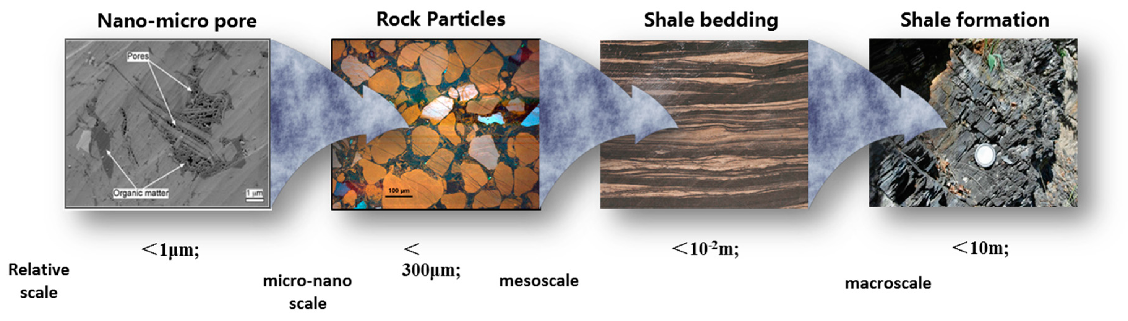
It has been commonly recognized that significant spatial heterogeneity, characterized by the multi-scale nature, extensively exists in shale reservoirs. The wetting properties and flow behavior of oil and gas change dramatically in different types of porous media. Cross-scale nano-micro porosity plays a dominant role in fluid storage, and micro-scale pore-throat morphology and connectivity strongly affected fluid transport phenomena. In addition, the fracture growth and the occurrence of natural fractures are extremely complex. Figure 1 shows multi-scale natural fractures, namely micrometer-scale (small scale), centimeter-scale (medium scale), and meter-scale (large-scale) fractures, co-exist in the shale reservoirs, of which the distribution pattern and occurrence both exhibit fractal features. Macro-scale favored flow areas are, accordingly, derived from the multi-scale connected/isolated natural fractures, localized accumulation of organic matter, and heterogeneous porous structure of shale reservoirs, which further affect the dynamic changes of pressures and fluid compositions in shale reservoirs. In addition, the complexity associated with reservoir, fracture, and fluid properties make various engineering techniques inaccurate to evaluate reservoir and fracturing properties of shales, such as sampling, well logging, and pressure-transient and rate-transient analysis [1,2]. However, compared with individual fractures, characterizing the complexity of multi-scale fracture networks still have many challenges.
To accurately capture of the fluid flow through the complex fracture network created by stimulation in unconventional reservoirs, previous studies focus on directly improving methodologies characterizing individual fractures for fracture networks. To the best of our knowledge, the existing models describing such complex systems are divided into three categories, including the dual-porosity model, the wire-mesh model, and the unconventional fracture model (UFM). The dual porosity model was first introduced by Warren and Root [3] to characterize the behavior of naturally-fractured reservoirs and is now widely applied in the shale gas fracture modeling [4,5,6,7]. Chaudhary [8] and Agboada et al. [9] simulate the fracture network with the help of logarithmic grid refinement, coupled with the dual porosity model, which is more flexible and able to offer a better description of pressure and saturation changes near the fracture. Hence, more accurate characterization of the flow pattern in the complex fracture network in the shale oil reservoir is obtained. By using the commercial simulator CMG, Odunuga [10] studied the self-similar reservoir fracture network fractal pattern and calculated the production capacity and drainage area of the fractured shale gas well with representative fractal patterns. The dual-porosity model is also used to shed light on the flow characteristics in shale gas reservoirs [11,12,13]. In the continuum media dual medium-based model, the fracture property is averaged and then assigned to each grid node, and it is generally reflected in the concept of the matrix and fracture, in which it is difficult to accurately characterize every detail of the complex fracture system. Carlson [14] studied the superior advantages of the discrete fracture model in dealing with the explicit fracture description of the non-continuum medium, which can provide more information concerning the inter-porosity flow, given that the fracture spacing is relatively large. A simplified discrete fracture model suitable for general-purpose reservoir simulators is presented to handle both 2D and 3D matrix-fracture systems [15]. Both the wire-mesh model and the unconventional fracture model originate from the discrete fracture model, which can explicitly describe the fracture network geometry based on fracture propagation. Xu et al. [16] established the wire-mesh model for hydraulic fracturing simulation, where there are two groups of planar fractures perpendicular to each other in the ellipse of the stimulated area. A new hydraulic-fracture model is developed to simulate the complex fracture-network propagation in a formation with pre-existing natural fractures proposed by Weng et al. [17]. The interaction, coupling, and deformation of hydraulic fractures and pre-existing natural fractures is taken into consideration in their model.
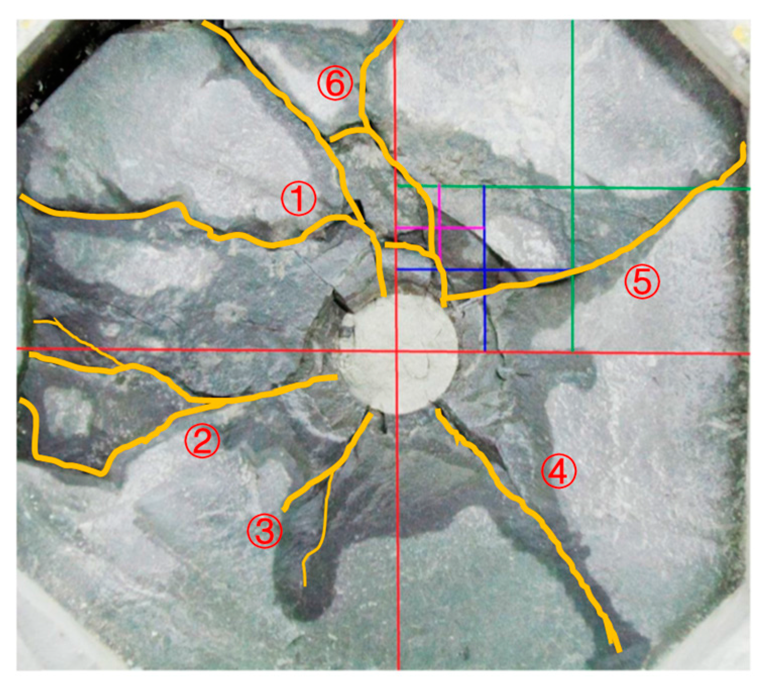
However, with the multi-scale features in particular shale reservoir, the guiding concept has changed from “bi-wing planar fractures” to “complex fracture networks”. To account for the clastic mass after fracturing, Guo et al. [18] conducted several fracture propagation experiments to evaluate the crushability, Figure 2. Al-Obaidy et al. [19] proposed “branched fractal” models that describe the pressure depletion in gas condensate shale reservoirs, and their results show that the fractal models allow for using more realistic shale permeability and improve the match for the observed trend. To capture part of the complexity of the fracture network, Mhiri et al. [20] introduced a novel approach to model the hydraulic fractures using “random-walk” stochastic method. The geometry of a fracture network is related to the fractal controlling parameters, and the multi-level bifurcated geometry of a fractal fracture better represents fractures of different orders and branches. Fuyong et al. [21,22] investigate fluid flow in fractal porous media and propose simulation method for the permeability of porous media based on the multiple fractal models.
The objective of this work is to apply fractal theory to model a multi-scale fracture system and provide a quantitative characterization of the induced hydraulic fracture networks. The fractal-fracture network model will be built to reflect the distribution pattern of the fractal-branching network based on the discrete fracture method. This approach is expected to give a more realistic representation of fracture geometry and multi-scale features observed in the unconventional reservoir. The findings of this research provide theoretical foundations for the characterization of the complex fracture network created by the multi-stage fracturing, while offering guidance for the production prediction.
2. Discrete Fractal-Fracture Network (DFFN)
2.1. Physical Model
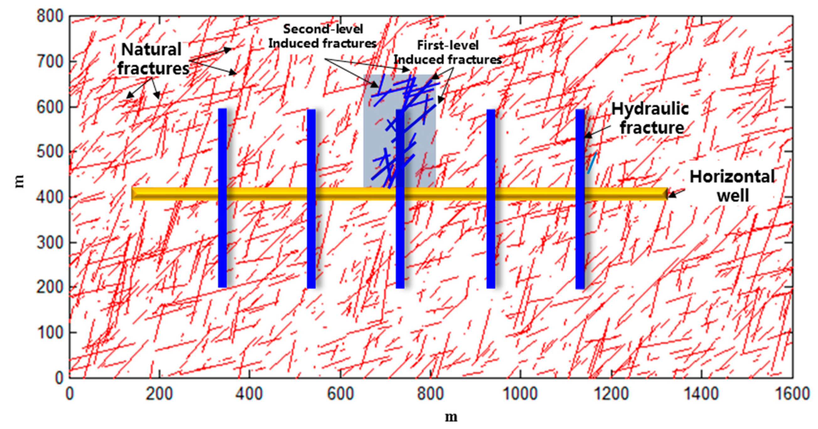
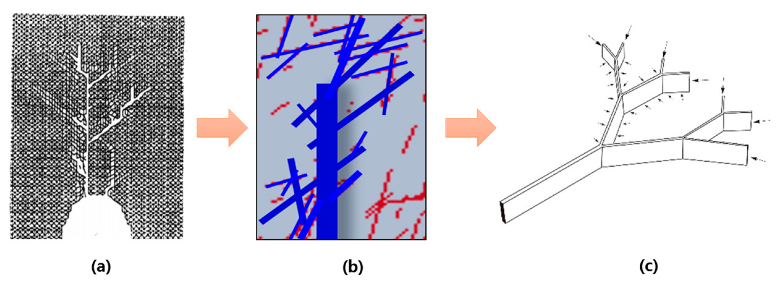
The fracturing treatment aims at creating the stimulated reservoir volume (SRV) to form the hydraulic fracture-natural fracture system [23,24,25,26]. However, without effective fracturing-forced propagation and openness, the natural fractures are very difficult to contribute to the production. Figure 3 shows a schematic plot of the fracture representative element volume (FREV), in which connected natural fractures and induced fractures are the main flow paths in the SRV, where permeability is much higher than the matrix. Given the process and relevant characteristics of the multi-stage hydraulic fracturing in unconventional reservoirs, the fractal fracture pattern is generated by construction theory [27] in Figure 4. Assumptions are made as follows: (1) Only the hydraulic fractures and natural fractures (including each level of induced fractures) connected with each other and isolated natural fractures are not considered. (2) Fractal fractures are generated hierarchically, and they are all perpendicular to the wellbore and grow by means of “bifurcation”. (3) Fracture properties stipulate in each level of the fractal fractures by scaling factors.
According to the fractal self-similar construction theory [27], the fractal dimension and the scaling factor of fractures can be determined. In terms of the symmetrically-distributed fracture network on each side of the main fracture, the branching fracture in the same level has the same length, while the branching fractures grow further following certain ratio factors. As hydraulic fractures propagate further, the fracture branch continuously increases, and the extended branching fractures become smaller than the previous cracks. Meanwhile, fracture properties, such as fracture width and fracture conductivity, with respect to each level, constantly decline. According to the deterministic self-similar fractal network, the branching fracture network is assumed to consist of N levels of branching fractures from the primary fracture to the secondary fracture, with a maximum fracture number of m. It is defined that the SRV of the secondary branching fractures and fracture network gradually decrease with the fracture propagation and, therefore, we introduced the concept of the stimulated fracture volume (SFV). The SFV of the fractal branching network is defined as being equal to the volume occupied by the fractures, which can be calculated by summarizing the effective stimulated volume of each level’s fractures.
where, represents the volume of the bifurcated fracture.
2.2. Mathematical Model of Discrete Fractal-Fracture Network
Following the mathematical model, we assumed a compressible single-phase fluid (i.e., oil) flow in the matrix and fracture systems, following Darcy’s law. The fractured horizontal well is located in the center area of the rectangular reservoir; multiple fractures with finite conductivity vertically cross the horizontal wellbore; the stimulated reservoir volume (SRV), distributed on the two sides of the fracture, is composed of the matrix/fracture medium. Dimensionless variables are defined, as follows:
where is the horizontal length, represent the distance to the boundary in x and y directions, respectively, are the dimensionless distances, is the matrix permeability, represents the fracture network permeability inside SRV, represents the hydraulic fracture permeability, and , , and represent the dimensionless permeability of the matrix, fracture network, and hydraulic fracture, respectively.
where is the dimensionless time, is the dimensionless pressure, is the flow capacity coefficient, and represents the storability ratio.
The motion equation for fluid flow in the matrix is:
where, is the flow velocity tensor in the matrix, 10−3 m/s; is the matrix pressure, MPa; and is the fluid viscosity, mPa·s. To account for the compressibility of rock and fluid, it is defined that .
2.2.1. Flow in the Matrix
To account for the formation matrix properties in both SRV and unstimulated reservoir volume, the surface source in three dimensions turns into a superposition of the line source in two-dimensional space. Then, we can obtain the dimensionless mathematical flow equation:
The boundary condition and initial condition can be written as follows:
2.2.2. Flow in Complex Fracture Network
With the assumptions of a pseudo-steady state flow between matrix systems and fracture systems, the exchange flow equation in dual-porosity region is presented as:
where is the natural fracture compressibility, MPa−1; represents the sink/source term in the complex fracture system; is the fracture network system pressure; is the porosity of natural fractures; represents the function of Delta, when , the function equals 1 and, otherwise, equals zero.
Initial condition:
Boundary condition:
represents the hydraulic fracture pressure, MPa.
The diffusivity equation with dimensionless variables can be written as follows:
The governing flow equations can be written by:
Initial condition:
2.2.3. Flow in the Hydraulic Fracture
The hydraulic fracture is regarded as a single-continuum medium and the diffusivity equation can be obtained as follows:
where is the hydraulic fracture compressibility, MPa−1; is the hydraulic fracture permeability, and qF represents the sink/source flow term in the hydraulic fracture.
Initial condition:
Boundary condition:
The dimensionless governing equation inside the hydraulic fractures is expressed as:
Based on triangular grids and the finite element method, a planar 2-D unsteady flow mathematical model is established in the article, and we solve the model by using the finite element method. Please refer to Appendix A for numerical solution details.
3. Results and Discussion
Based on the discrete fractal fracture model (DFFM), the effects of the fracture pattern and conductivity on the well performance are analyzed. The numerical model built for the representative element volume of the fracture is applied to estimate the performance following every iteration stage, which assumes that the homogeneous reservoir and each staged fractal fracture are open, and the existing natural fractures are not modeled. Since conductivity declines further from fracture networks [29,30], the multi-scale conductivity is also considered in the simulation.
3.1. Fractal Fracture Network Pattern
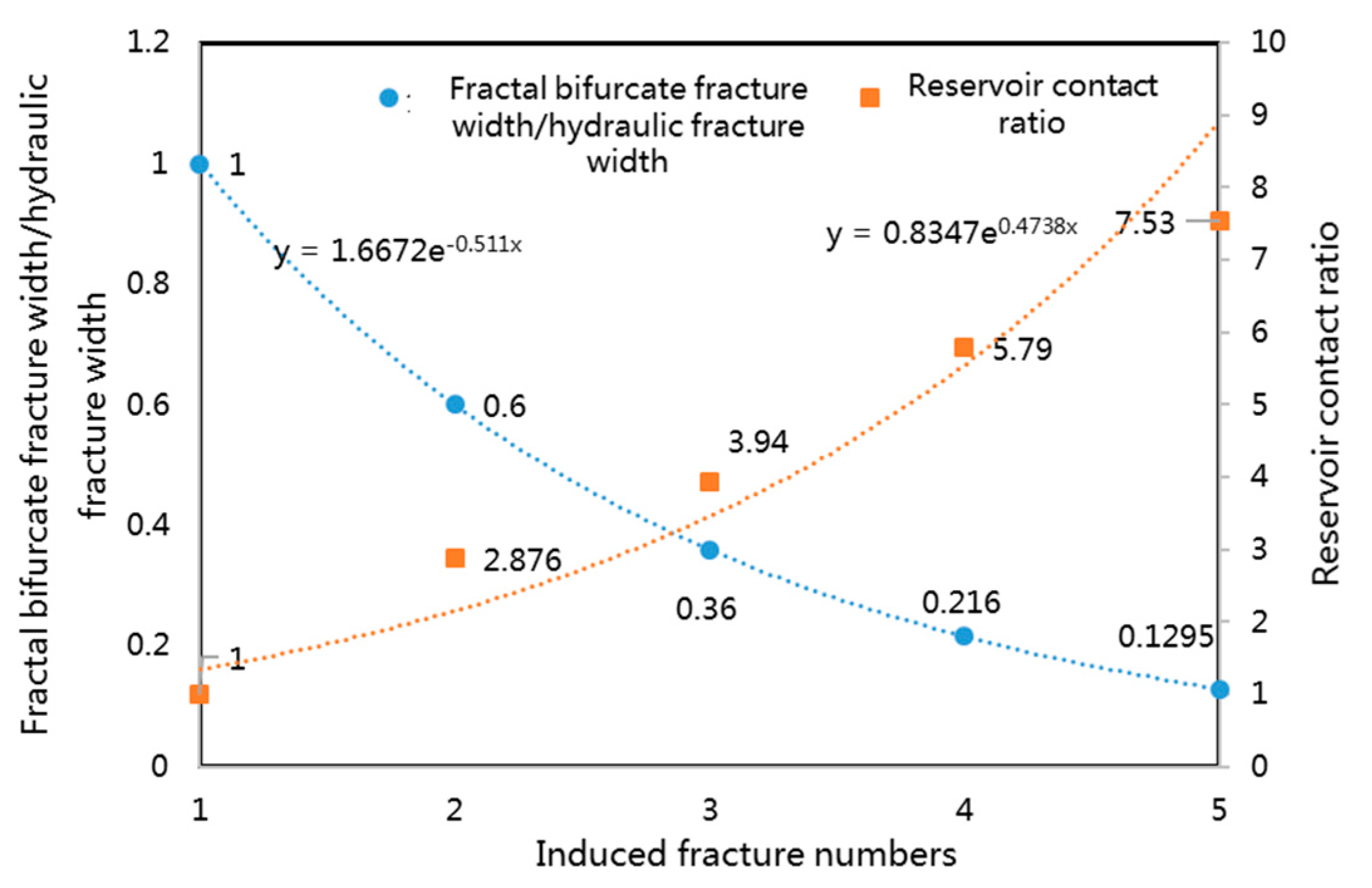
With the fractal branching fracture propagation, hydraulic fractures encounter natural fractures and divert to form next-level branching fractures. The fracture bifurcation pattern is created via numerical programming, and the fracture geometry is illustrated in Figure 5. The connectivity for each branching fracture varies, with the initial hydraulic fracture conductivity of 200 D·cm. After five iterations, the value decreases to 2.4 D·cm, which only accounts for 12% of the main fracture. Figure 6 shows the fracture width and reservoir contact area, as well as the induced fracture numbers, which indicates that with increasing induced fracture numbers (the fracture network becomes more complex further away), even the fractal bifurcation width decreases evidently, but it leads to exponential growth of the reservoir contact area.
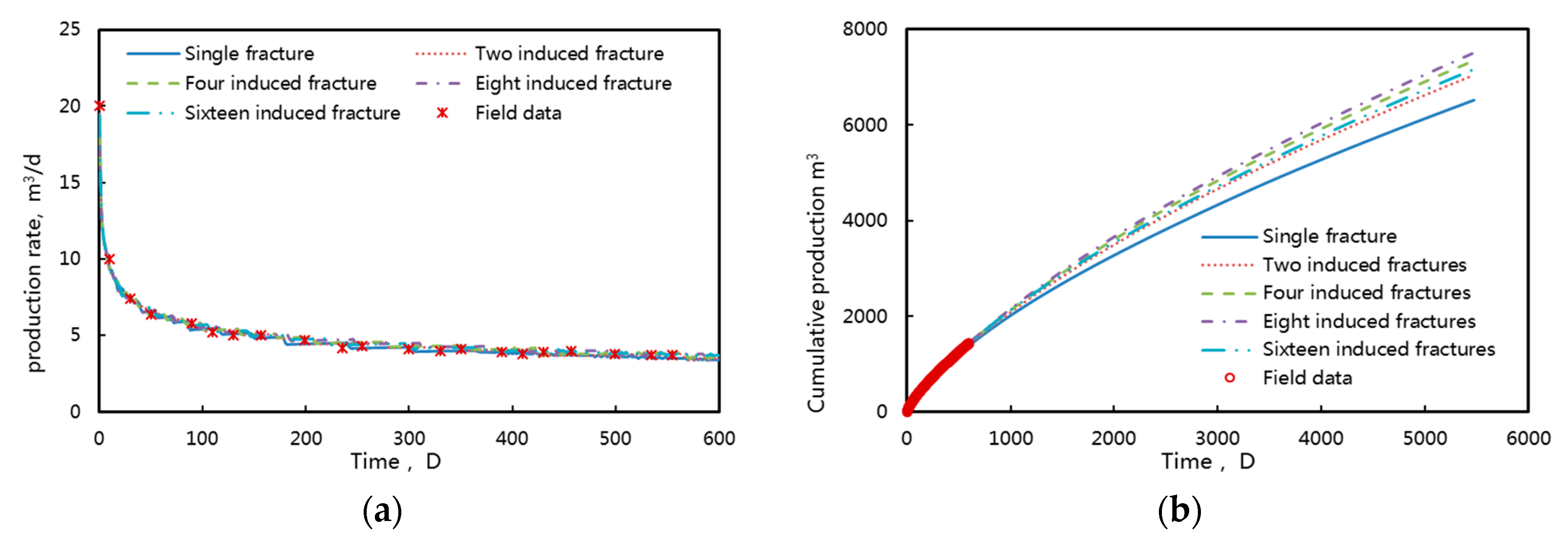
The actual production data from the Changqing oil field are used for history matching so as to validate the proposed model, and the result is shown in Table 1. After generating the fractal fracture cases, all five models are found to give similar daily production in the previous two years. Induced fractal fracture geometry varies significantly, and the well performance remains very close (Figure 7a). However, the induced fracture model predicates much higher cumulative volumes in the next 15 years, and the production volume with eight induced fractures estimated from this model is 20% larger than that from a single fracture (Figure 7b), which indicates the great contribution of the induced fracture network to the well performance in the late production stage.
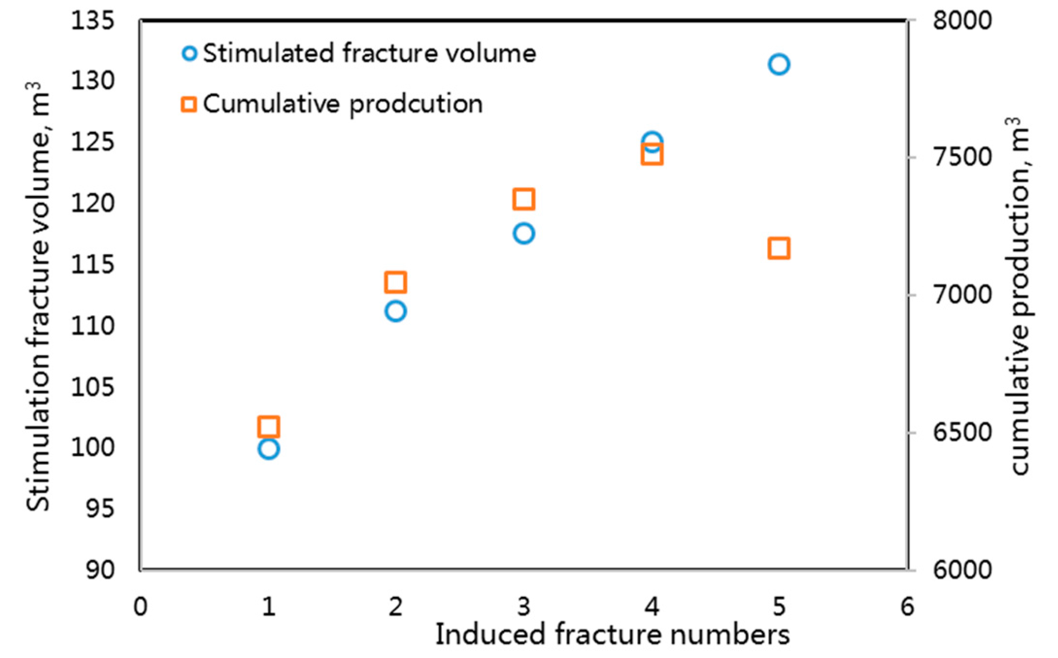
Figure 8 shows the stimulated fracture volume (SFV) and cumulative oil production change with respect to the induced fracture numbers. The complexity of the fracture network rises with the stimulated fracture volume of branching fractures. Higher induced fracture numbers can generate more complicated networks, but they also bring strong interference between the connected induced fractures, which can lead to a production decrease in the end.
3.2. Multi-Scale Fractal Fracture Network Conductivity
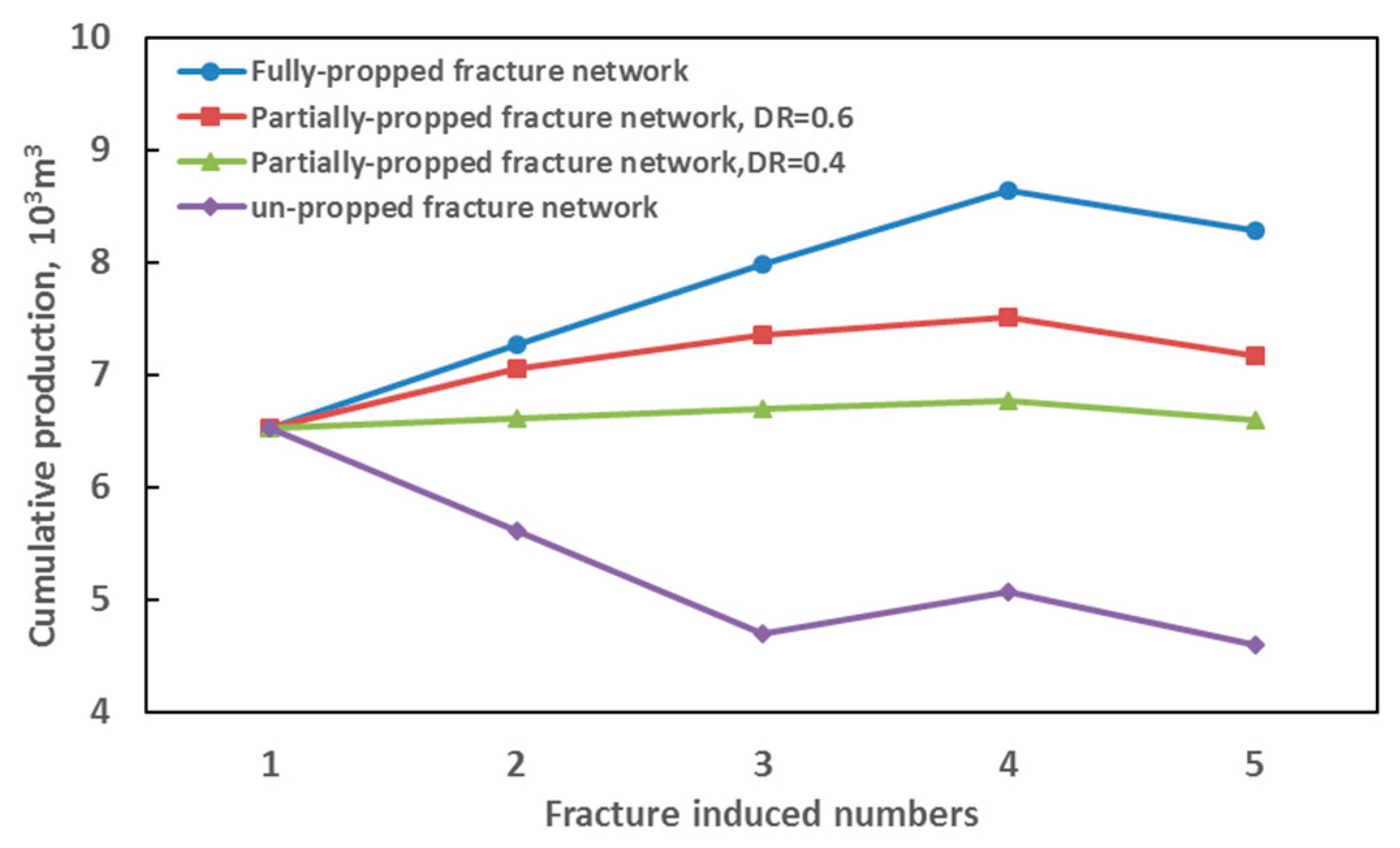
Due to the features of brittle, naturally-fractured shale formations, massive shear failure occurs during hydraulic fracturing. When the rough rock surface encounters shear slippage, it cannot restore to original status and shear-induced permeability is maintained, which is known as the “self-propped” fracture network. In order to investigate the effect of multi-scale conductivity, fracture conductivity is considered to decrease with the bifurcation, which means the natural decrease of fracture conductivity from the primary fracture to the secondary and tertiary branches (Figure 9). The fully-propped fracture network refers to the case where the proppants can be transported to the secondary fracture network far from the wellbore. The partially-propped case means that after the fracturing fluid is pumped into the formation, the proppants can only migrate near the primary fracture and massive “self-propped” fracture networks are generated at distant fracture systems. Meanwhile, the conductivity of the fracture network gradually declines as proppants break, migrate, or block the formation. In terms of the un-propped fracture network, the main fracture is effectively propped, while the secondary fracture and tertiary branches are only self-propped, which means no more proppant migration in the fracture networks.
Based on the fracture geometry in Figure 5, we propose a model to investigate the effects of fracture propped patterns (Table 2) on cumulative oil production. The result shows that cumulative oil production of the fully-propped fracture network greatly exceeds that of the other two propped patterns. This indicates that the models with arbitrarily propped fracture geometry are superior to the single fracture. The partially-propped fractures’ cumulative oil volume decreases significantly due to the decline of the fracture permeability and fracture width. Figure 10 also indicates that with the rapid decrease of complex fracture conductivity, the cumulative production increases slightly with growing complexity of the fracture network. Therefore, improving the effective conductivity of the fracture network is the precondition for hydraulic fracture stimulation.
Regarding the un-propped fracture model, the cumulative production fluctuation according to the geometry, topological structure, and tortuosity of the fracture network can cause extra fluid flow resistance while the fracture network conductivity is relatively low. Without the propped network in the stimulated reservoir volume, the primary fracture is the main contributor to production. The decrease of the main fracture length is bound to have a great impact on fracture production, and also connected, induced, complex fractures interfering with each other can lead to lower performance.
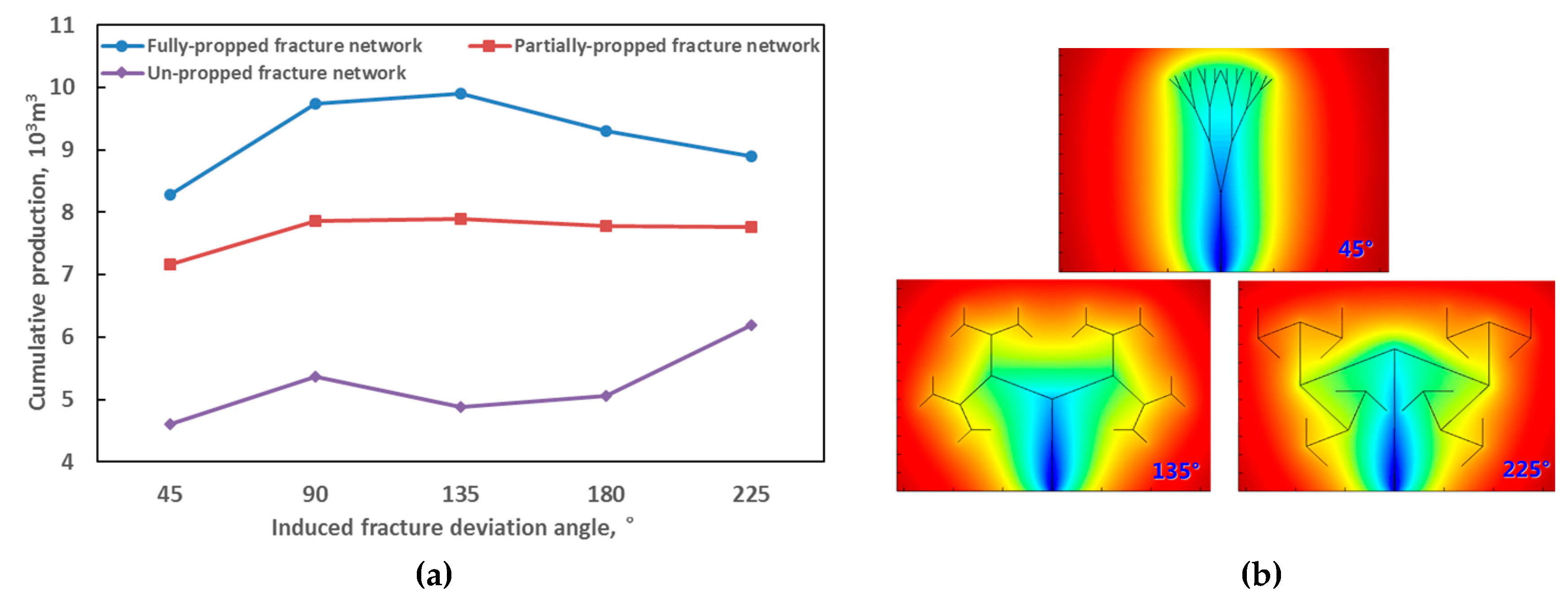
We also investigate he cumulative production with different induced fracture deviation angles (Figure 11). It is illustrated that the reservoir contact area of the fracture network increases with the bifurcation angle (deviation angle). When fractures are featured by high conductivity, it is inappropriate to create a denser network in the stimulated reservoir volume, and only a few interweaving fractures can result in very good performance. The cumulative oil production of the partially-propped fracture case is fairly close to the others, and the effect of fracture morphology on yield is not great. When it comes to lower conductivity fractures, the effect of the main fracture substantially overweighs the secondary and tertiary fractures.
4. Conclusions
This paper investigates the fractal characteristics of the complex fracture network created by multi-stage fracturing in shale reservoirs. It has been found that discrete fractal-fracture network (DFFN) models allow for using more realistic fracture values to evaluate the well performance. (1) We establish the numerical simulation model for fractal fracture network characterization. The proposed model meshes with the unstructured grid, which is solved using the finite element method. (2) We proposed a new method for fractal fracture network characterization according to the construction theory. (3) The correlation between multi-scale fractal fracture patterns, conductivity, and corresponding production has been quantitatively analyzed with the help of the mathematical formula. The proposed research may provide valuable insight into optimal hydraulic fracturing design and unconventional resource recovery maximization. For future extensions, a stochastic-based fractal fracture network combined with micro-seismic events may be coupled to quantify the complex network fractures; this will improve hydraulic fracture design and production performance.
Acknowledgments
This work is supported by National Natural Science Foundation of China (51674279), National Basic Research Program of China (2014CB239103), China Postdoctoral Science Foundation funded project (2016M602227), Natural Science Foundation of Shandong (ZR201709200376), the Fundamental Research Funds for the Central Universities (18CX02168A), and the National Science and Technology Major Project (2017ZX05049-006). The authors appreciate the reviewers and editors for their critical and helpful comments.
Author Contributions
Wendong Wang, Yuliang Su, and Bin Yuan designed the theoretical framework and wrote the manuscript; Kai Wang and Xiaopeng Cao conducted the simulations and analyzed the data; and all authors have read and approved the final manuscript.
Conflicts of Interest
The authors declare no conflicts of interest.
Nomenclature
| L | Lateral length of horizontal well, m |
| N | Directions, x, y, and z |
| Distance to boundary in x-direction, m | |
| Distance to boundary in y-direction, m | |
| Dimensionless distance to x boundary | |
| Dimensionless distance to y boundary | |
| Permeability of reservoir matrix, m | |
| Permeability of fracture networks in SRV, mD | |
| Permeability of hydraulic fractures, mD | |
| Dimensionless permeability of reservoir matrix | |
| Dimensionless permeability of fracture networks in SRV | |
| Dimensionless permeability of hydraulic fractures | |
| Time, s | |
| Dimensionless time | |
| Dimensionless pressure | |
| Flow capacity coefficient | |
| Storability ratio | |
| Fluid flow velocity tensor in reservoir matrix, 10−3 m/s | |
| Original reservoir pressure, MPa | |
| Pore pressure of reservoir matrix, MPa | |
| Pressure in hydraulic fractures, MPa | |
| Pressure in complex fracture network system, MPa | |
| Fluid viscosity, mPa·s | |
| Reservoir porosity | |
| Original reservoir porosity | |
| Natural fractures porosity | |
| Fluid density, kg/m3 | |
| Original fluid density, kg/m3 | |
| Pore compressibility coefficient, MPa−1 | |
| Natural fracture compressibility coefficient, MPa−1 | |
| Hydraulic fracture compressibility coefficient, MPa−1 | |
| Fluid compressibility coefficient, MPa−1 | |
| volume flow rate in unit volume, s−1 | |
| Sink/source term in complex fracture system, s−1 | |
| Sink/source flow term in hydraulic fracture, s−1 | |
| Delta function. It equals to 1 when M = M’, otherwise, it equals to zero. |
Appendix A. Numerical Solution of Mathematical Model
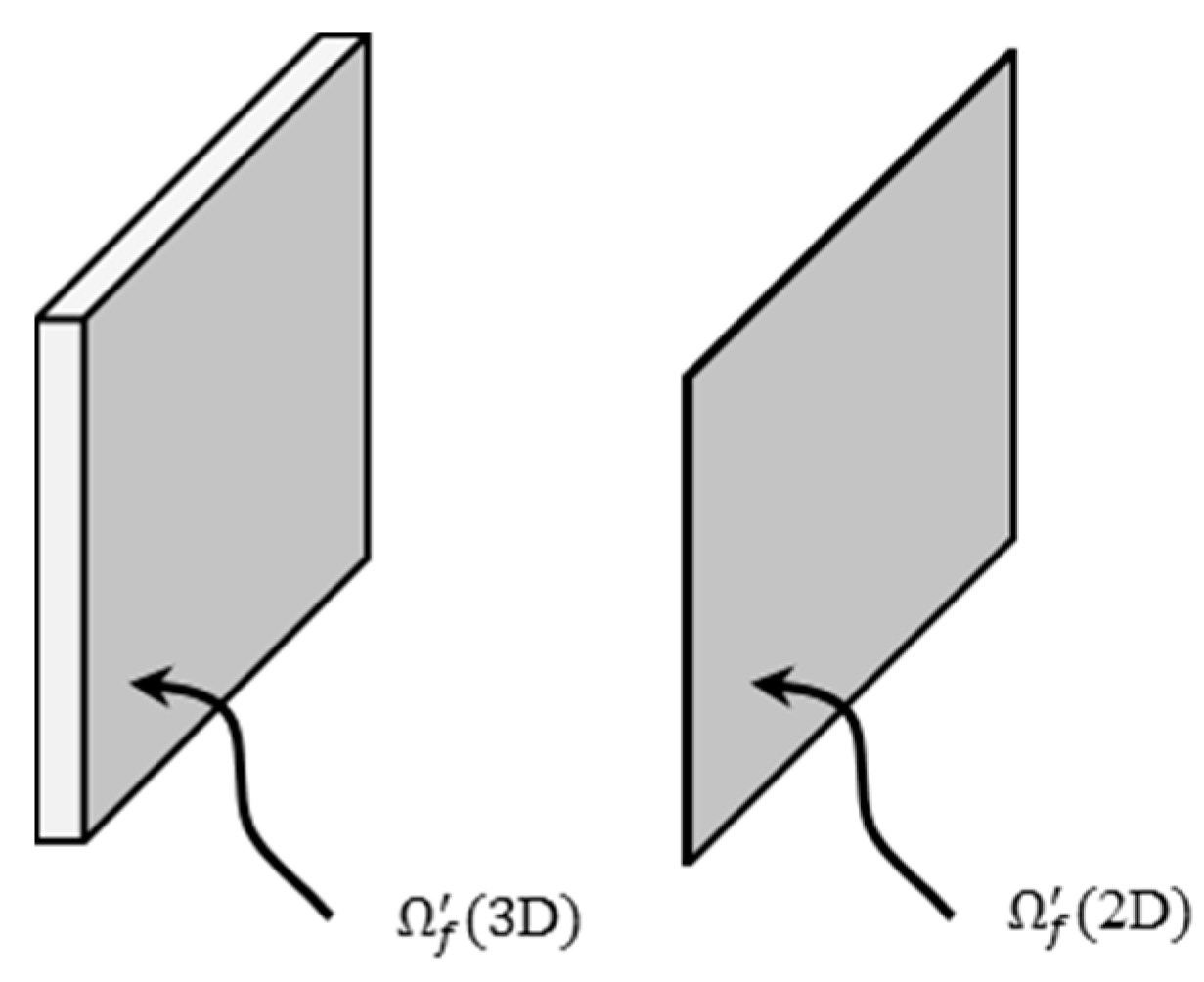
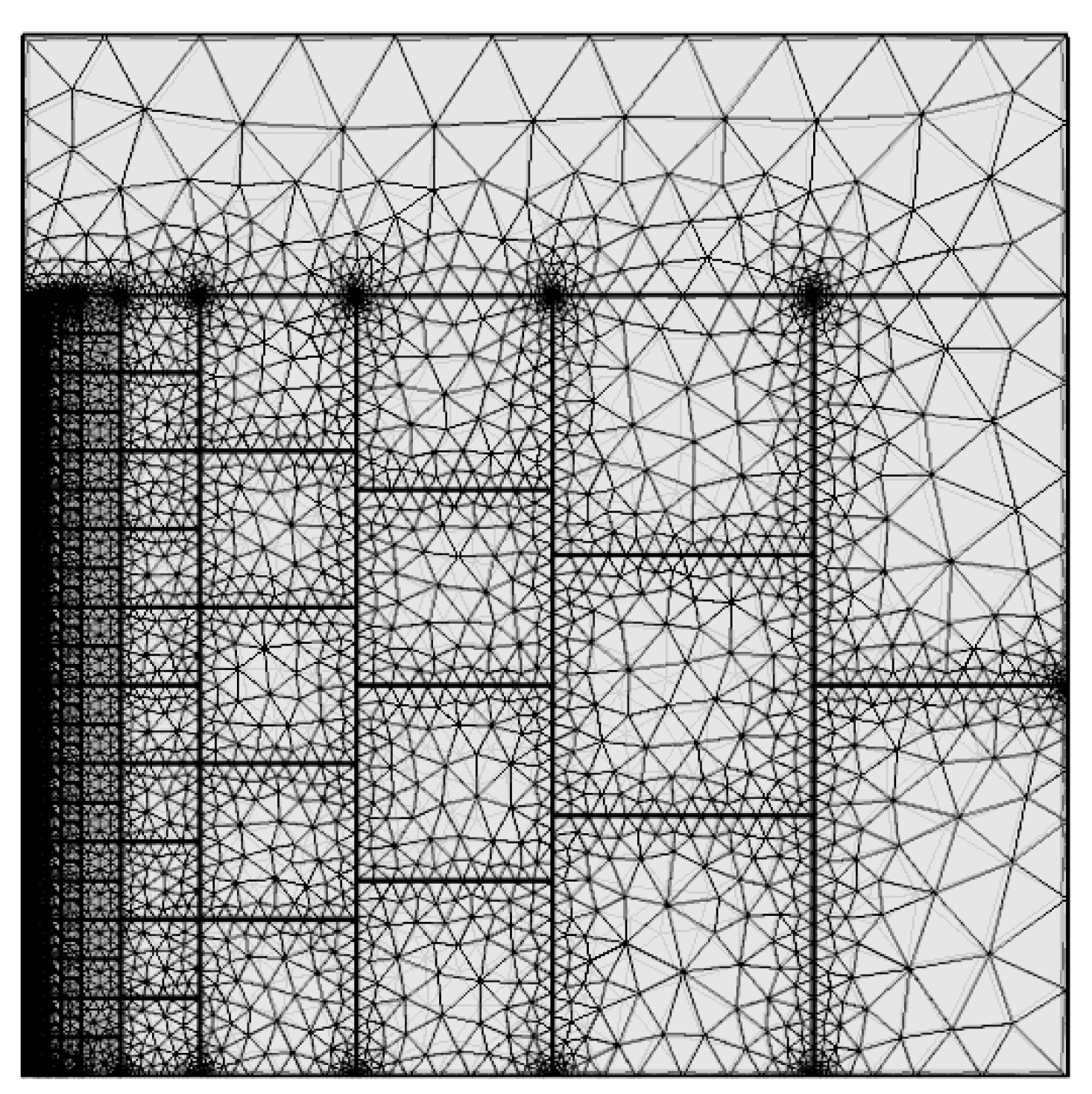
The fractures are treated explicitly based on the discrete fracture model, considering the properties of hydraulic fractured horizontal well, SRV, and reservoir unit [31]. The characteristic analysis is carried out for the reservoir matrix, SRV, and hydraulic fractures, respectively. The Galerkin method of weighted residuals is applied to establish the finite element integral equation, which makes continuous infinite degrees of freedom to solution unit discrete into the finite element [32,33,34]. The grid blocks on the horizontal well and fracture are made to be dense, employing a triangular frontier advancement meshing algorithm (gridblocks around the horizontal well are shown as Figure A1 and Figure A2). Dimensions of hydraulic fractures are reduced based on the discrete fracturing model, which makes 3D fractures equivalent to 2D fractures with a certain degree of dimensionless width. Additionally, fluid flow in fractures, which obey the Navier-Stokes equation, is equivalent to be compliant with Darcy’s law.
Figure A1.
The 3D fracture volume is equal to the 2D fracture surface.

Figure A2.
Grid meshing generated for FDFN (2D).

We assume that reservoir consists of unstimulated reservoir matrix , stimulated reservoir volume and hydraulic fractures , and the following equation can be derived by integration:
where can be expressed as , and is the dimensionless fracture width.
By applying interpolation function in the element, and the dimensionless pressure in element “s” can be expressed as:
where is the dimensionless pressure in the element, and represents the corresponding interpolation function at node i in the element. In this paper, we use the linear polynomial interpolation function:
The approximate solution of differential fluid flow equations is derived using the Galerkin method of weighted residuals.
The tetrahedron characteristic matrix of the reservoir matrix is expressed as:
where , and .
Similarly, the tetrahedron characteristic matrix of SRV can be obtained as:
where , and .
In a similar way, the 2D hydraulic fracture characteristic matrix is:
where is the width of the primary fracture, equals , , and .
We combine the above characteristic matrices of different regions to obtain the matrix of the whole reservoir, and simplify the equation sets according to the obtained matrix elements and the corresponding serial numbers. The equation sets are discrete by backward differentiation on the timescale. In this paper, the triangle mesh grid and adaptive mesh subdivision technology are adopted in the model and we demonstrate that the results converge to a solution and are independent of mesh size. Refinement of the mesh has no effect on the solution.
References
- Bin, Y.; Moghanloo, R.G.; Da, Z. A novel integrated production analysis workflow for evaluation, optimization and predication in shale plays. Int. J. Coal Geol. 2017, 180, 18–28. [Google Scholar]
- Zhiyuan, W.; Baojiang, S.; Xiaohui, S. Calculation of temperature in fracture for carbon dioxide fracturing. SPE J. 2016, 12, 1491–1500. [Google Scholar]
- Warren, J.E.; Root, P.J. The behavior of naturally fractured reservoirs. SPE J. 1963, 3, 245–255. [Google Scholar] [CrossRef]
- Du, C.M.; Zhang, X.; Zhan, L.; Gu, H.; Hay, B.; Tushingham, K.; Ma, Y.Z. Modeling hydraulic fracturing induced fracture networks in shale gas reservoirs as a dual porosity system. In Proceedings of the Society of Petroleum Engineers International Oil and Gas Conference and Exhibition in China, Beijing, China, 8–10 June 2010. [Google Scholar]
- Li, J.; Du, C.; Zhang, X. Critical evaluation of shale gas reservoir simulation approaches: Single-porosity and dual-porosity modeling. In Proceedings of the Society of Petroleum Engineers SPE Middle East Unconventional Gas Conference and Exhibition, Muscat, Oman, 31 January–2 February 2011. [Google Scholar]
- Zimmerman, R.W.; Chen, G.; Hadgu, T.; Bodvarsson, G.S. Numerical dual-porosity model with a semi-analytical treatment of fracture/matric flow. Water Resour. Res. 1993, 29, 2127–2135. [Google Scholar] [CrossRef]
- Chong, Z.; Li, X.; Chen, X.; Zhang, J.; Lu, J. Numerical investigation into the effect of natural fracture density on hydraulic fracture network propagation. Energies 2017, 10, 914. [Google Scholar] [CrossRef]
- Chaudhary, A.S.; Ehlig-Economides, C.A.; Wattenbarger, R.A. Shale oil production performance from a stimulated reservoir volume. In Proceedings of the SPE Annual Technical Conference and Exhibition, Denver, CO, USA, 30 October–2 November 2011. [Google Scholar]
- Agboada, D.; Ahmadi, M. Production decline and numerical simulation model analysis of the Eagle Ford shale play. In Proceedings of the SPE Western Regional & AAPG Pacific Section Meeting Joint Technical Conference, Monterey, CA, USA, 19–25 April 2013. [Google Scholar]
- Odunuga, A.B. Investigating Drainage Patterns of Shale Production as a Function of Type Fracture System in the Reservoir; University of Oklahoma: Norman, OK, USA, 2012. [Google Scholar]
- Zhang, X.; Du, C.; Deimbacher, F.; Crick, M.; Harikesavanallur, A. Sensitivity studies of horizontal wells with hydraulic fractures in shale gas reservoirs. In Proceedings of the International Petroleum Technology Conference, Doha, Qatar, 7–9 December 2009. [Google Scholar]
- Cipolla, C.L.; Lolon, E.; Mayerhofer, M.J. Reservoir modeling and production evaluation in shale-gas reservoirs. In Proceedings of the International Petroleum Technology Conference, Doha, Qatar, 7–9 December 2009. [Google Scholar]
- Daobing, W.; Hongkui, G.; Xiaoqiong, W.; Jianbo, W.; Fanbao, M.; Yu, S.; Peng, H. A novel experimental approach for fracability evaluation in tight volcanic rock gas reservoirs. J. Nat. Gas Sci. Eng. 2014, 23, 239–249. [Google Scholar]
- Carlson, E.S.; Latham, G.V. Discrete Network Modeling for Tight Gas Fractured Reservoirs; Society of Petroleum Engineers: Richardson, TX, USA, 1993. [Google Scholar]
- Karimi-Fard, M.; Durlofsky, L.J.; Aziz, K. An efficient discrete-fracture model applicable for general-purpose reservoir simulators. SPE J. 2004, 9, 227–236. [Google Scholar] [CrossRef]
- Xu, W.; Thierceiin, M.J.; Ganguly, U. Wiremesh: A novel shale fracturing simulator. In Proceedings of the International Oil and Gas Conference and Exhibition in China, Beijing, China, 8–10 June 2010. [Google Scholar]
- Weng, X.; Kresse, O.; Cohen, C.E.; Wu, R.; Gu, H. Modeling of hydraulic fracture network propagation in a naturally fractured formation. SPE Prod. Oper. 2011, 26, 368–380. [Google Scholar] [CrossRef]
- Guo, T.; Zhang, S.; Ge, H. A new method for evaluating ability of forming fracture network in shale reservoir. Rock Soil Mech. 2013, 34, 947–954. (In Chinese) [Google Scholar]
- Al-Obaidy, R.T.I.; Gringarten, A.C.; Sovetkin, V. Modeling of Induced Hydraulically Fractured Wells in Shale Reservoirs Using “Branched” Fractals. In Proceedings of the SPE Annual Technical Conference and Exhibition, Amsterdam, The Netherlands, 27–29 October 2014. [Google Scholar]
- Mhiri, A.; Blasingame, T.A.; Moridis, G.J. Stochastic Modeling of a Fracture Network in a Hydraulically Fractured Shale-Gas Reservoir. In Proceedings of the SPE Annual Technical Conference and Exhibition, Houston, TX, USA, 28–30 September 2015. [Google Scholar]
- Wang, F.; Liu, Z.; Jiao, L.; Wang, C.; Guo, H. A Fractal Permeability Model Coupling Boundary-layer Effect for Tight Oil Reservoirs. Fractals 2017, 25, 1750042. [Google Scholar] [CrossRef]
- Xia, Y.; Cai, J.; Wei, W.; Hu, X.; Wang, X.; Ge, X. A New Method For Calculating Fractal Dimensions of Porous Media Based On Pore Size Distribution. Fractals 2017. [Google Scholar] [CrossRef]
- Huang, J.-I.; Kim, K. Fracture process zone development during hydraulic fracturing. Int. J. Rock Mech. Min. Sci. Geomech. Abstr. 1993, 30, 1295–1298. [Google Scholar] [CrossRef]
- Wang, Y.; Li, X.; He, J.; Zhao, Z.; Zheng, B. Investigation of fracturing network propagation in random naturally fractured and laminated block experiments. Energies 2016, 9, 588. [Google Scholar] [CrossRef]
- Bin, Y. Nanofluid pre-treatment, an effective strategy to improve the performance of low-salinity waterflooding. J. Pet. Sci. Eng. 2017. [Google Scholar] [CrossRef]
- Zhao, Y.; Shan, B.C.; Zhang, L.H. Seepage flow behaviors of multi-stage fractured horizontal wells in arbitrary shaped shale gas reservoirs. J. Pet. Sci. Eng. 2016, 13, 1–10. [Google Scholar] [CrossRef]
- Xu, P.; Yu, B.; Feng, Y.; Liu, Y. Analysis of permeability for the fractal-like tree network by parallel and series models. Phys. A Stat. Mech. Appl. 2006, 369, 884–894. [Google Scholar] [CrossRef]
- Wang, W.; Su, Y.; Zhang, X.; Sheng, G. Analysis of the complex fracture flow in multiple fractured horizontal wells with the fractal tree-like network models. Fractals Complex Geom. Patterns Scaling Nat. Soc. 2015, 23, 1550014. [Google Scholar] [CrossRef]
- Yuan, B.; Moghanloo, R.G.; Wang, W. Using nanofluids to control fines migration for oil recovery: Nanofluids co-injection or nanofluids pre-flush? A comprehensive answer. Fuel 2018, 215, 474–483. [Google Scholar] [CrossRef]
- Mayerhofer, M.J.; Lolon, E.; Warpinski, N.R.; Cipolla, C.L.; Walser, D.W.; Rightmire, C.M. What is stimulated reservoir volume? SPE Prod. Oper. 2010, 25, 89–98. [Google Scholar] [CrossRef]
- Zhang, T.; Li, Z.; Adenutsi, C.D.; Caspar, D.A.; Li, F. A new model for calculating permeability of natural fractures in dual-porosity reservoir. Adv. Geo-Energy Res. 2017, 1, 86–92. [Google Scholar] [CrossRef]
- Nezhad, M.M.; Javadi, A.A. Stochastic finite element approach to quantify and reduce uncertainty in pollutant transport modeling. ASCE J. Hazard. Toxic Radioact. Waste Manag. 2011, 15, 208–215. [Google Scholar] [CrossRef]
- Nezhad, M.M.; Javadi, A.A.; Rezania, M. Finite element modelling of contaminant transport considering effects of micro and macro heterogeneity of soil. J. Hydrol. 2011, 404, 332–338. [Google Scholar] [CrossRef]
- Niessner, J.; Helmig, R. Multi-physics modeling of flow and transport in porous media using a downscaling approach. Adv. Water Resour. 2009, 32, 845–850. [Google Scholar] [CrossRef]
Figure 1.
Multi-scale heterogeneity of reservoir system in shale reservoirs.

Figure 2.
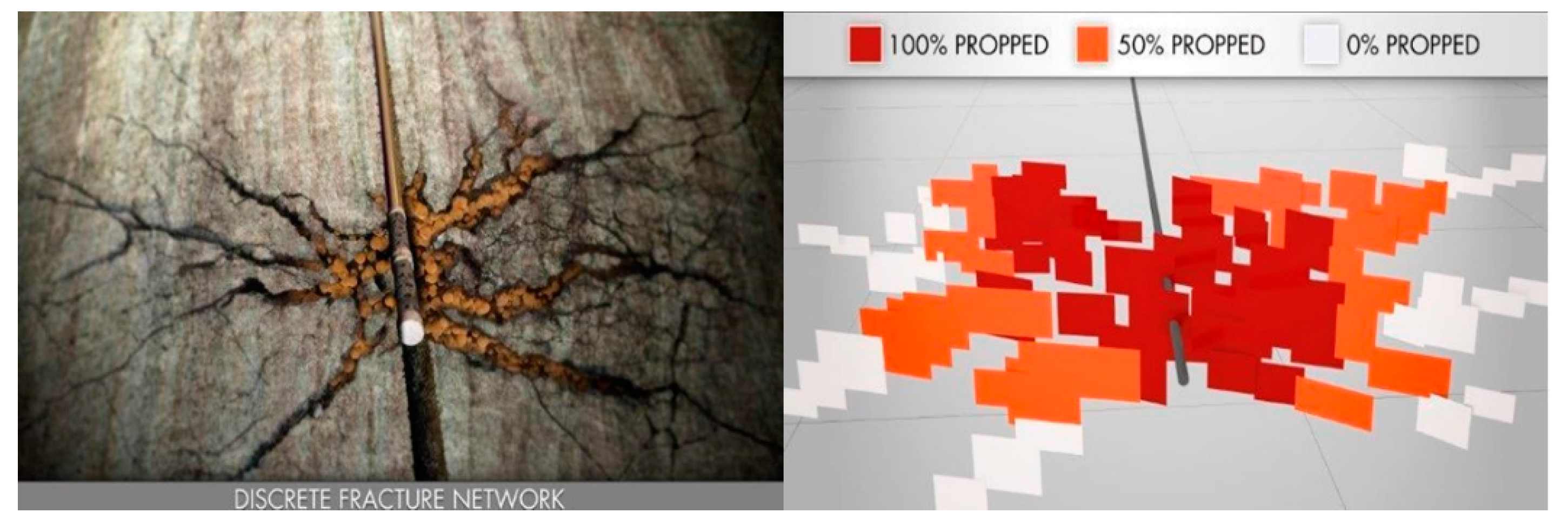
Core fracture network experiment result. A total of six cracks are generated after fracturing. ④ and ⑤ grow only single fractures perpendicular to the wellbore, but ①, ②, ③, and ⑥ split into two branches after propagating a few centimeters, modified from Guo et al. [18]
Figure 2.
Core fracture network experiment result. A total of six cracks are generated after fracturing. ④ and ⑤ grow only single fractures perpendicular to the wellbore, but ①, ②, ③, and ⑥ split into two branches after propagating a few centimeters, modified from Guo et al. [18]

Figure 3.
Multi-stage fractured horizontal well with representative element volume (dark area).

Figure 4.
Determined self-similar fractal fracture model by construction theory. (a) represent branching fracture propagation geometry, modified from [23]; (b) represent the fracture representative element volume in Figure 2; (c) is determined Y-shape self-similar fractal fractures [28].

Figure 5.
Fractal geometry design for one stage (bifurcation angle is 45°).

Figure 6.
Fractal fracture width and reservoir contact area change with respect to induced fracture numbers.
Figure 6.
Fractal fracture width and reservoir contact area change with respect to induced fracture numbers.

Figure 7.
Fractal fracture network history matching combined with Changqing oil field data. (a) represent production rate with respect to different induced fracture scenario; (b) represent the cumulative production for all cases.
Figure 7.
Fractal fracture network history matching combined with Changqing oil field data. (a) represent production rate with respect to different induced fracture scenario; (b) represent the cumulative production for all cases.

Figure 8.
Stimulated fracture volume and cumulative oil production change with respect to induced fracture numbers.
Figure 8.
Stimulated fracture volume and cumulative oil production change with respect to induced fracture numbers.

Figure 9.
Schematic plot for a propped discrete fracture network.

Figure 10.
Cumulative production comparison among fractal bifurcate fracture with respect to different fracture network conductivity.
Figure 10.
Cumulative production comparison among fractal bifurcate fracture with respect to different fracture network conductivity.

Figure 11.
Cumulative production comparison among fractal bifurcate fracture geometries with respect to different fracture network conductivity. (a) reflect the cumulative production changed with induced fracture deviation angle; (b) represent the pressure distribution at the end of simulation.
Figure 11.
Cumulative production comparison among fractal bifurcate fracture geometries with respect to different fracture network conductivity. (a) reflect the cumulative production changed with induced fracture deviation angle; (b) represent the pressure distribution at the end of simulation.


Table 1.
Changqing oil field data.
| Parameter, Symbol, Unit | Value |
|---|---|
| Fracture unit in the x, m | 300 |
| Fracture unit in the y, m | 200 |
| Reservoir thickness, m | 19 m |
| Matrix permeability, D | 2.3 × 10⁻⁴ |
| Matrix porosity | 0.108 |
| Matrix compressibility, pa−1 | 3.75 × 10⁻¹⁰ |
| Main fracture conductivity, D·cm | 200 |
| Main fracture porosity | 0.000015 |
| Fracture compressibility, pa−1 | 3.75 × 10⁻⁸ pa−1 |
Table 2.
Different propped fracture network scenario and parameters.
| Scenario | Induced Fracture Permeability, D (Fracture Width) | Schematic Plot | |||||
|---|---|---|---|---|---|---|---|
| Main (5 cm) | Second (3 cm) | Third (1.8 cm) | Fourth (1.08 cm) | Fifth (0.648 cm) | |||
| Fully-propped fracture network | 2 | 2 | 2 | 2 | 2 |  | |
| Partially-propped fracture network | DR * = 0.6 | 2 | 1.2 | 0.72 | 0.432 | 0.259 |  |
| DR = 0.4 | 2 | 0.8 | 0.32 | 0.128 | 0.0512 |  | |
| Un-propped fracture network | 2 | 0.0512 | 0.0512 | 0.0512 | 0.0512 |  | |
* DR is declined ratio of fracture permeability, whose value equals the ratio of the secondary fracture permeability over the previous fracture permeability.
© 2018 by the authors. Licensee MDPI, Basel, Switzerland. This article is an open access article distributed under the terms and conditions of the Creative Commons Attribution (CC BY) license (http://creativecommons.org/licenses/by/4.0/).
Share and Cite
MDPI and ACS Style
Wang, W.; Su, Y.; Yuan, B.; Wang, K.; Cao, X. Numerical Simulation of Fluid Flow through Fractal-Based Discrete Fractured Network. Energies 2018, 11, 286. https://0-doi-org.brum.beds.ac.uk/10.3390/en11020286
AMA Style
Wang W, Su Y, Yuan B, Wang K, Cao X. Numerical Simulation of Fluid Flow through Fractal-Based Discrete Fractured Network. Energies. 2018; 11(2):286. https://0-doi-org.brum.beds.ac.uk/10.3390/en11020286
Chicago/Turabian StyleWang, Wendong, Yuliang Su, Bin Yuan, Kai Wang, and Xiaopeng Cao. 2018. "Numerical Simulation of Fluid Flow through Fractal-Based Discrete Fractured Network" Energies 11, no. 2: 286. https://0-doi-org.brum.beds.ac.uk/10.3390/en11020286
Note that from the first issue of 2016, this journal uses article numbers instead of page numbers. See further details here.