Article

The Conductive and Predictive Effect of Oil Price Fluctuations on China’s Industry Development Based on Mixed-Frequency Data

1
School of Economics and Management, Xidian University, Xi’an 710126, China
2
Nanjing University of Information Science & Technology, Jiangsu Talents Research Base, Nanjing 210044, China
3
Department of Management Sciences, City University of Hong Kong, Hong Kong 999077, China
4
Department of Decision Sciences, College of Business and Economics, Western Washington University, Bellingham, WA 98225, USA
*
Author to whom correspondence should be addressed.
Submission received: 1 May 2018 / Revised: 21 May 2018 / Accepted: 25 May 2018 / Published: 28 May 2018
(This article belongs to the Special Issue Energy Economy, Sustainable Energy and Energy Saving)

Abstract

:
Presently, the total supply of crude oil is sufficient, but short-term supply and demand imbalances and regional imbalances still exist. The effect of crude oil supply security and price impact cannot be ignored. As the world’s largest oil importer, China is highly dependent on foreign oil. Therefore, the fluctuation of international oil prices may impact the development of China’s various industries in a significant and differential way. However, because the available data have different frequencies, much of the recent research that addresses the effect of oil prices on industry development need to replace, split, or merge the original data, resulting in loss of the information from the original data. Using the mixed data sampling model (MIDAS(m,K,h)-AR(1)) with the first-order lag autoregressive terms of the interpreted variables, this study builds a mixed data model to investigate the effect of oil price volatility on the output of China's industries. This study expands the extant research by financial market fluctuations and macroeconomic analysis, and at the same time makes short-term predictions on the output of China’s seven main industries. The analysis results show that the mixed data regression model brings the original information contained in different frequency data into the model analysis, and utilizes the latest high frequency data of the explanatory variables to perform real-time short-term prediction of low-frequency interpreted variables. This method improves the timeliness of forecasting macroeconomic indicators and the accuracy of short-term forecasts. The empirical results show that the spot price of international crude oil has a significant and differential impact on the outputs of the seven industries in China. Among them, oil price fluctuation has the greatest impact on the output of China’s financial industry.

1. Introduction

The IEA’s World Energy Outlook 2017 report states that oil, natural gas, and coal are still the world's leading energy sources by 2035, and it expects that oil demand will continue to grow at an average annual rate of 0.7%. By the early 2030s, the non-fuel use of petroleum (especially the petrochemical industry) will become the main source of oil demand growth. The report concludes that “the world is not yet ready to say goodbye to the oil era”. Therefore, studying the impact of oil price fluctuation on the macro-economy will still have high practical value for a long time to come.
The impact of the international oil price on the macro economy has always been a hot and difficult topic for academic research. All previous fluctuations of international oil prices had huge impacts on the global economy [1]. A 2004 study by the International Energy Agency showed that the oil price increased from 25$ to 35$ per barrel. In the first two years of this rising oil price period, the total GDP of OECD countries fell by 0.4%, and the inflation rate increased by 0.5%. Simultaneously, the unemployment rate increased, and the world GDP declined by an average of at least 0.5%. The impact of high oil prices on oil-importing developing countries was even more serious. For every $10 rise of price per oil barrel, Asian economic growth rate dropped by 0.8 percentage points in that period. As the world's largest oil importing developing country, China will be affected more by the fluctuation of international oil price, and the impact of the fluctuation of the international oil price on various industries will have different reaction. Therefore, there are great theoretical and practical values in studying the impact of international oil price fluctuation on different industries in China.
The current research on the effect of oil price on the macro-economy focuses more on analyzing the effect of oil price fluctuation on the total economic indicators [2,3,4]. Only a few studies have investigated the differential impact of oil prices on different industries. The research on the effect of oil price on macro-economy using mixed frequency data is even scarcer. The economic system is a complex system within which subsystems interact with each other. Except for the correlation between indicators measured with the same-frequency statistics, the indicators measured with mixed-frequency statistics representing different economic significance also influence each other, and the application of such a case is broader, which needs more attention from the academia.
Because of the different statistical frequencies of data (for example, GDP is reported quarterly CPI and PPI data monthly, financial market returns daily, stock market fluctuation intraday, etc.), researchers are often confronted by the difficulty in exploring the true effect of oil price on the economy because most existing models are based on the same-frequency data. In response to this problem, some scholars use alternative indicators that have the same data frequency as the explanatory variables [5]; some use the method of adding or replacing to convert high frequency data to low frequency data [6]; and others choose interpolation to process low-frequency data as high-frequency data [7]. However, these data processing methods can easily overlook the completeness of data substitution in the process of data replacement, resulting in the loss (or increase) of the original data information. Therefore, to a certain extent, it will lead to inaccurate model estimation. The mixed data model solves the above problems.
This study constructs an econometric model that can comprehensively use quarterly and monthly data, that is, a mixed-frequency sampling model with first-order lag autoregressive terms of the interpreted variables [8]. The impact of the international crude oil spot price on the output of seven industries in China is analyzed. Based on the model, the latest high-frequency data of the international oil price is used to make real-time short-term forecasts on the outputs of the seven industries in China. The models and research ideas adopted in this study have the following characteristics and advantages: Firstly, the direct use of monthly and quarterly data avoids the loss of information in original data and artificial data formation caused by converting the mixed frequency data into the same frequency data. Secondly, we propose an analysis of the impact of the international oil price fluctuation on the development of various industries in China in the context of mixed-frequency data, which is the first in the literature, to the best of our knowledge. This analysis can not only capture changes in various industries, but also capture the coordinated changes in macroeconomic aggregates. Thirdly, this study proposes to use the non-restrictive Beta weight function in which there is no restriction on the weight function parameters, in order to observe the relative superiority of the MIDAS model. This weight function is different from the weight functions that are used in the existing mixed data sampling models. Finally, this study constructs a nonlinear least squares model with first-order lag autoregressive terms of explanatory variables that can play an important role in comparative analysis, and further enhance the superiority of the mixed-frequency data sampling model over the same-frequency data sampling model.

2. Literature Review

A mixed data model can make full use of various frequency raw data to build models. Two well-established mixed data models are the Mixed Data Sampling (MIDAS) model and Mixed Vector Autoregressive Moving Average (VARMA) model. The MIDAS model was proposed by Ghysels et al. [9] based on the distributed lag model. The original intention is to use the MIDAS model to obtain information from high-frequency financial data to predict the volatility of the financial market. The study also uses the MIDAS model to validate the hypothesis that the higher risk of stocks is often accompanied by the higher-yield. Asgharian et al. [10] applied the GARCH (Generalized AutoRegressive Conditional Heteroskedasticity)-MIDAS model to test whether the microvariables can predict short-term and long-term financial market fluctuations in the variance of the yield. The results show that the high-frequency micro-information contained in the GARCH-MIDAS model can improve the prediction accuracy, especially the prediction accuracy is higher in predicting the long-term fluctuation. Pan et al. [11] introduced the GARCH-MIDAS model to study the relationship between oil price fluctuations and macroeconomic fundamentals. The empirical results show that structural mutation leads to a higher degree of GARCH implicit volatility persistence. The GARCH-MIDAS model is significantly superior to a single econometric model for out-of-sample forecasting of oil price fluctuation. More and more scholars have begun to study the MIDAS model.
Other scholars have applied the MIDAS model to the analysis and prediction in many other fields. In particular, the mixed-frequency vector autoregressive model has been widely applied in the macroeconomic field. For example, Clements et al. [12,13] used monthly macroeconomic and financial indicators to forecast quarterly GDP growth rate. Frale et al. [14] used Factor-Mixed Data regression model (FaMIDAS) to predict Italian quarterly GDP based on monthly macroeconomic indicators, such as PMI, M2, and foreign trade indices. Andreou et al. [15] used the FaMIDAS model to predict the growth rate of US quarterly GDP and examined the feasibility and practicality of using the daily financial data to predict low-frequency GDP, such as quarterly GDP, in the MIDAS model. Foroni et al. [16] introduced the Mixed-Frequency Vector Autoregressive (MF-VAR) model, discussed the estimation and inference of the Markov-switching Mixed-Frequency Vector Autoregressive (MSMF-VAR) model, and applied the MSMF-VAR model to the forecast of GDP growth and the analysis of the turning point in economic cycles in the euro zone. The results show that the MSMF-VAR model is valid for estimating the cyclical state of economic activity. In their study of whether financial high-frequency data can help predict the true price of the oil market, Baumeister et al. [17] stated that the MIDAS model is superior to the real-time MF-VAR model in terms of the accuracy of predicting oil price using high-frequency financial data.
The MIDAS model has also attracted the interests of Chinese scholars. Liu H. et al. [18] used the MIDAS model for forecasting quarterly GDP in China. Through comparative analysis with the baseline model (OLS (Ordinary Least Squares), PDL (Polynomial Distributed lag), AR (Autoregressive) and ADL (Autoregressive Distributed Lag) models), they found that MIDAS model has accurate comparative advantage in short-term prediction and analysis of China's macroeconomic aggregate. Geng et al. [19] used M-MIDAS-DL model and quarterly GDP real-time data to establish the China’s quarterly GDP forecasting model. The model accurately predicts the decline and rebound trend of China’s economic growth rate since 2008, which can provide leading signals for decision makers. Zheng et al. [20] constructed a data measurement model of China's quarterly and monthly economic cycle, namely, the dynamic factor model for the transfer of mixed-frequency data region, to measure the economic cycle of China. The empirical results show that the dynamic factor model for the transfer of mixed-frequency data can not only capture the changes in China's economic cycles, but also extract a consistent index based on the mixed data. The dynamic model has good reliability and timeliness in predicting China’s economic cycles (economic turning point identification and measurement). Li et al. [21] used Markov switching mixed frequency data sampling (MS-MIDAS) model with China’s monthly and quarterly economic data to monitor China’s economic cycles. The empirical results show that China’s economic cycles have the characteristics of three-zone periodic changes. Additionally, the duration of the different zones is asymmetric, which proved that the MS-MIDAS model can timely and accurately predict China’s economic cycles. Jiang et al. [22] attempted to use a dynamic mixed data model to predict China’s GDP growth. The empirical results show that compared with the traditional prediction methods, the forecasting accuracy of the dynamic factor model with mixed predicting variables and data has better accuracy. In addition, the combined forecasting can further improve prediction performance.

3. Model Introduction

3.1. Introduction to the MIDAS Model

3.1.1. Basic MIDAS Regression Model

The univariate MIDAS (m, K) model proposed by Ghysels et al. [9] can directly integrate the low-frequency data y t and high-frequency data x t ( m ) into the following regression model by using parameterized polynomial weights W ( L l / m ; θ ) :
y t = α + β W ( L l / m ; θ ) x t ( m ) + ε t
where, ε t ~N(0, σ 2 ), y t denotes the t-th low-frequency response variable, x t denotes the t-th high-frequency explanatory variable, t denotes the time of low-frequency data, and m denotes the number of the high-frequency data of t-th period. If y t is quarterly data and x t is monthly data, then m = 3, W ( L l / m ; θ ) is a weighted delay polynomial, and there is W ( L l / m ; θ ) = k = 1 K ω ( k ; θ ) L k l / m , where L l / m is a lag operator and satisfies L l / m x t ( m ) = x t l / m ( m ) , l = 0, 1, ..., K − 1, K is the high-frequency data lag order used to parameterize the weight function. W ( k ; θ ) can take different forms of weighting function.

3.1.2. h-Step Forward-Prediction MIDAS (m,K,h) Model

The forward-prediction MIDAS (m,K,h) in h-step is a single equation direct prediction model with succinct parameters, which has the advantages of real-time forecasting and correction in comparison with the traditional intra-frequency prediction model. Its specific form is:
y t = α + β W ( L l / m ; θ ) x t h / m ( m ) + ε t

3.1.3. h-Steps Forward-Prediction MIDAS(m,K,h)-AR(1) Model

Under normal circumstances, the time series of macroeconomic variables often have autocorrelation relationship due to the inertia of the economic system. The empirical study of Stock and Watson [23] shows that the prediction results of predictive models containing only explanatory variables were only about 5% better than the autoregressive models. Therefore, this study sets a model of MIDAS(m,K,h)-AR(1) with the autoregressive lag of the first-order autoregressive terms of the interpreted variables for the specific research object. The specific form is as follows:
y t = α + λ y t 1 + β W ( L l / m ; θ ) x t h / m ( m ) + ε t

3.2. Weight Function Selection and Setting

The determination of the weight polynomial function in the mixed data regression model is very important. The appropriate mathematical functions and statistical methods need to be used to determine the weight polynomial function. The right mathematical functions and statistical methods can transform high-frequency data to data sets that includes a large amount of information, eliminate microscopic noise of high-frequency data, and avoid the information loss caused by the traditional method that directly transforms high-frequency data into lower-frequency data before modeling. In actual analysis, according to the features of fewer parameters and convergence in the weight function, many estimation parameters of high-frequency explanatory variables in the model are expressed by functions, which makes it possible to directly introduce high-frequency explanatory variables into the model.
In the MIDAS model, the commonly used weight functions include Almon polynomial function, Exponent Almon polynomial function, Beta function, etc. The Almon polynomial function is mostly used in the prediction and analysis of financial market fluctuation. The Exponent Almon polynomial function and Beta function are used in macroeconomic analysis and forecasting. Based on the problems studied in this paper, the limitations of the function form and the practical operability, the Beta function is chosen as the weight function of this study. The specific form of the Beta function is:
W j t = Z j θ 1 1 ( 1 Z j ) θ 2 1 i = 0 K Z i θ 1 1 ( 1 Z i ) θ 2 1 + θ 3
where, Z j = j 1 k 1 . The Beta function is very flexible. It can construct weighting functions of ascending, descending, flat, convex and U-shaped. The specific form depends on the parameters ( θ 1 , θ 2 , θ 3 ) of the Beta weight function.
In addition, the selection of high-frequency data lag polynomials is also a key issue that needs to be addressed in this study. Ghysels et al. [9] thought that using non-linear estimation method to optimize the parameter θ in the weight function of the MIDAS regression equation, and obtained the optimal length of the lag order by estimating the weight function graph of the parameter θ ^ . The lag order determination method is data-driven, so the lag order is optimal. However, in the applied research in the field of macroeconomics, the choice of lag order has the characteristics of arbitrariness and experientiality, and some scholars choose the lag order according to information criteria (such as AIC and BIC criteria).

4. Modeling and Empirical Analysis of Mixed-Frequency Data Regression Model for Macroeconomic Impact Effect of Oil Price Fluctuation

MIDAS was introduced into China in 2007 by Xu et al. [24] Since then more and more scholars have applied the MIDAS model in studying China’s macroeconomic and financial fields because of its relative advantages in using high-frequency data to build models. However, prior studies using the MIDAS focused more on a single market [3,4,25]. There was little empirical study on the linkage between China’s macroeconomic and financial markets. Also based on the MIDAS method, this study attempts to examine the effect of the oil price fluctuation on the output of various industries in China. We construct a MIDAS-based forecasting model for various industries in China to assess the impact of oil price and make short-term predictions on the output of various industries in China.

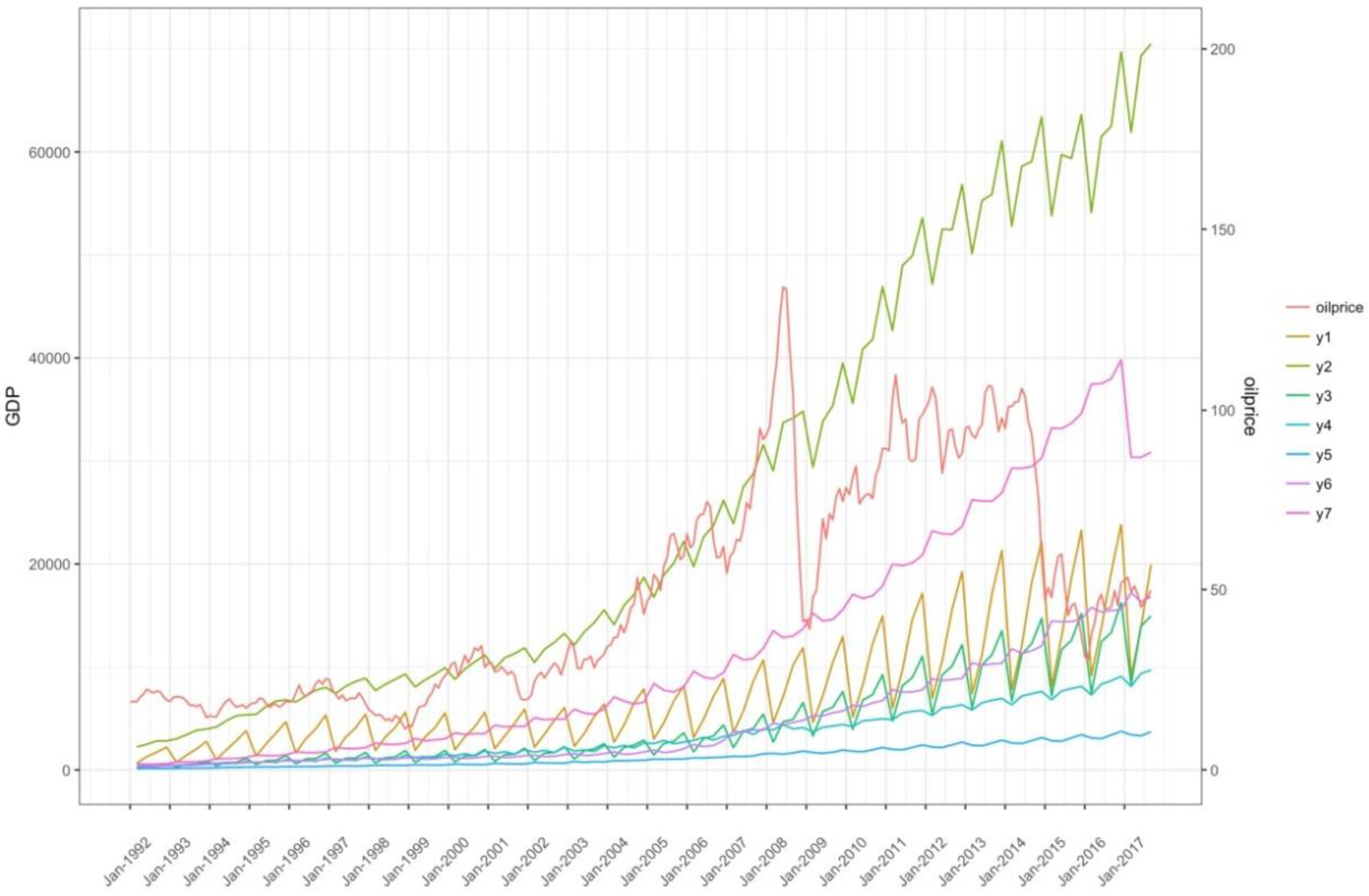
4.1. Indicator Selection and Data Description

We select the spot price index of the monthly West Texas Intermediate(WTI) crude oil from January 1992 to September 2017 as the explanatory variable. The explained variables of this study include quarterly data indicators such as the output of agriculture, forestry, animal husbandry and fishery ( y 1 ), industrials output ( y 2 ), output of construction industry ( y 3 ), transportation and warehousing and postal output ( y 4 ), accommodation and catering output ( y 5 ), financial industry output ( y 6 ) and other industry output ( y 7 ). We construct the non-restrictive Beta weight function MIDAS(m,K,h)-AR(1) model to analyze the differentiated impacts of the spot price fluctuation of the international crude oil on various industries in China. In order to eliminate the heteroscedasticity of the model, logarithmic processing is applied to all data.
The main reason for using the mixed frequency data in the study is due to the data availability from different sources. The highest statistical frequency of China’s macroeconomic indicators of GDP from China’s National Bureau of Statistics is quarterly. Whereas, the international crude oil spot price is only available in monthly and annual format. We believe that the annual oil price itself is smoothed out of its seasonality, periodicity, volatility, etc., losing too much sample information, therefore, annual oil price is not a good predicative variable for the model. In addition, weekly data and daily data do not well reflect the cyclical nature of the oil price fluctuation. So, monthly oil price is a good choose for the model.
China’s GDP accounting includes eleven industries, but the data record interval is two years for the industry of information transmission, software and information technology services and the industry of rental and business services, whereas the interval for other industries is twenty-five years. In order to use a consistent data interval for the analysis, these two industries are excluded from the analysis. The study sets 12 as the maximum lag period for the Beta weight function of the MIDAS model. In the empirical analysis process, we found that within the maximum lag time of the Beta weight function, the model did not delete a reasonable lag order for the wholesale and retail industry and the real estate industry, so we excluded these two industries too from the model. With these considerations, the final number of industries included in this study is seven.
Figure 1 shows that the outputs of the various industries, especially the industrial sector ( y 2 ), and the oil price have the same increasing trend. During the financial crisis, the oil price fell sharply, resulting in a decline in the output of various industries, but the decline was short and small. After the financial crisis, the oil price fluctuation were full of complexity, but the outputs of various industries showed a trend of growth over the same period. After 2017, there was a slight drop in the oil price, and the outputs of industries, such as industrial industry, construction, and finance, also showed large or small decreases. This chart can only objectively reflect the trend fluctuations in some segments. Due to the inconsistency of data frequency, the specific analysis is explained in depth in the section of empirical analysis.

4.2. Empirical Analysis Based on MIDAS(m,k,h)-AR(1) Model

This study selects the Beta weight function to construct the MIDAS class model, which sets no restriction on the number of parameter and the parameter range. We set the maximum lag order to 12 for the lag period of the weight function. In the empirical analysis process, the lag order of the low frequency variable and the high frequency variable is eventually determined according to the t and F statistic. Finally, the optimal model is obtained by comparing the prediction accuracy index: the root mean square error (RMSE), the average absolute error (MAE), the average absolute value of the error percentage (MAPE) the average absolute percentage error (SMAPE), and the Taylor U statistic. We use the model to describe the effects of oil price fluctuation on various economic variables, the final model is as follows:
y i , t = α i + λ i y i , t 1 + β i , j j = 1 12 ω i , j / m θ X i , t j m m + ε i , t
The variable y i , t represents the output of different industries in the t-th period, and X t j m m represents the relatively high-frequency international crude oil spot price index in the lag period, ω i , j / m θ is the weight function of the parameter θ. The estimated results of the specific parameters are shown in Table 1.
From the results of the sampling model for the mixed-frequency data, the output changes in China’s different industries have certain inertia (warping effect), that is, the output of an industry in current period is significantly affected by the output in the previous period, and the impact effect reaches 0.977215 on average. The results also show that the international oil price has a positive impact on China’s various industries, that is, the rise in the oil price is associated with the rise in the output of various industries in China.
Among the seven industries in China, the oil price fluctuation has the greatest impact on the output of the financial industry, and the dynamic total multiplier effect reaches 0.035997. That is, when the oil price changes by 1%, it will cause a change of 3.5997% in China’s financial industry output. Because petroleum is the world's most important strategic resource among all fossil energy sources, the strengthening of its strategic attributes and metal properties makes the oil financial market become an important global financial trading platform. When the international crude oil price fluctuates, through global financial market it will affect the China’s financial market, gold market, stock market, and foreign exchange market, then affect all aspects of the macro economy in China. Therefore, the financial industry has become the most affected industry by the oil price volatility. The rise in oil price reflects an increase in global energy demand and the growth of the economy, therefore, further activates the global financial market. In China, which has the highest share of the global oil net imports, when oil price rises, the financial industry output must increase. It also illustrates the sensitivity and importance of the financial market in the process of global integration.
The dynamic total multiplier effect of the international oil price fluctuation on China’s transportation, warehousing, and postal services is 0.004356. That is, when the oil price changes by 1%, it will cause a 0.4356% change in the output of China’s transportation, warehousing, and postal services. As the main fuel for transportation, oil has a significant impact on the industry. As of 2015, the oil consumption of the transportation industry accounted for 37.25% of the total domestic oil consumption. Rising crude oil prices will increase transportation and logistical costs, resulting in a decline in corporate profit, which is detrimental to the development of company. After 2008, the oil price has stabilized with fewer fluctuations, and the impact on the transportation, warehousing, and postal services has gradually decreased. The rise in oil price theoretically has a negative impact on China’s transportation, warehousing, and postal services. However, because China’s necessary demand for oil is still large and the economic growth accompanied by the rising oil price will help the development of the industry, the overall effect should be that the increase in the oil price would be accompanied by the increase in the output of the industry.
The dynamic total multiplier effect of the international oil price fluctuation on China’s agriculture, forestry, animal husbandry, and fishery industry is 0.024132. That is, when the oil price changes by 1%, it will cause a change of 2.4132% in the output of China’s agriculture, forestry, animal husbandry, and fishery. Because the fluctuation in crude oil price will affect the price of ethanol and diesel, the rise of oil price will increase the cost of agricultural machinery used in irrigation, ploughing, transportation, fertilizers, pesticides, and plastic films. However, the economic growth accompanying the rise of oil price will stimulate the consumption of crops, such as corn and soybeans. At the same time, the increase in the price of crude oil will cause the increase in the cost of agricultural resources, resulting in a trend of rising price of agricultural products, especially basic crops, such as rice, maize, and wheat, thereby increasing the output of agriculture, forestry, animal husbandry, and fishery.
The dynamic total multiplier effect of the international oil price fluctuation on China’s industrials industry is 0.022763. That is, when the oil price changes by 1%, it will cause a 2.263% change in the output of China’s industrials sector. Crude oil as the basic energy is related to many industries. Various derivatives of crude oil (such as gasoline, diesel, kerosene, fuel oil, etc.) are closely related to many aspects of the industrial operation. Its importance is self-evident. As China’s oil is a resource-restricted industry, domestic crude oil supply is far from meeting domestic demand for crude oil. Many products from many industries, such as petroleum processing, chemical raw materials and chemicals, chemical fiber manufacturing, and chemical products, are produced from the raw petroleum or petroleum preliminary products. The oil industry is at the end of the large industrial chain where oil industry is the starting point. Therefore, the rise of the crude oil price and the price of petroleum preliminary products in the upper stream of the chain will affect the down-stream chemical industry. Also, the synthetic fiber products in the chemical fiber manufacturing industry are mainly made of petroleum and natural gas. The rise of oil price also has a certain impact on the profit of the industry. Therefore, in theory the impact of the rising oil price on China’s industrial sector should be negative. However, economic growth accompanied by the rise of oil prices may also stimulate the development of the industry. Thus, overall effect of the increase in oil prices may be positive on the output of the industrial sector.
The dynamic total multiplier effect of international oil price fluctuation on China’s accommodation and catering industry is 0.034992, that is, when the oil price changes by 1%, it will cause a 3.4192% change in the output of China’s accommodation and catering industry. Due to the transformation of the economic environment and the conductive mechanism of oil price in economic life, any signs of oil price fluctuation will affect the cost of living of residents through transportation, agriculture, and manufacturing, and indirectly lead to an increase in the cost of accommodation and catering. Theoretically, the impact of the rising oil price on China’s accommodation and catering industry should be negative, but the economic growth accompanied by the rise of oil price may also stimulate the development of the industry. Therefore, the overall effect of the rising oil price may also have positive effect on the output of the industry. Table 1 also shows that the dynamic total multiplier effect of the international oil price fluctuation on China’s accommodation and catering industry is greater than the dynamic total multiplier effect on industrial industries. Since 2015, China’s tertiary industry has contributed to GDP more in terms of absolute value and contribution rate than the secondary industry. Because the rise of the tertiary industry is more positively driven by economic development, the rise of the tertiary industry objectively reflects the change of the China’s economic structure.
The dynamic total multiplier effect of the international oil price fluctuation for other industries is 0.033026. That is, when the oil price changes by 1%, it will cause 3.3026% change of the output of all economic sectors except agriculture, forestry, animal husbandry and fishery, industry, construction, transportation, warehousing and postal services, accommodation and catering, and finance. It shows that the extensiveness of the use of crude oil as a strategic commodity and commercial product and the importance of the fluctuation of crude oil price to social and economic life.
In summary, oil price is still an important driver of China’s economic growth and influencing economic restructuring. Currently China’s domestic crude oil price is in line with the international oil price. Although the price of domestically refined oil products is influenced by China’s specific national conditions, the impact of the international oil price fluctuation on the volatility of China’s domestic oil prices can be mitigated to some extent. However, the fluctuation of China’s domestic oil price can influence the country through investment, consumption, and other channels, affecting China’s domestic economy.

4.3. Parameter Estimation Results and Fitting Accuracy Analysis

The Beta weight function contains three parameters to be evaluated. We can often limit the Beta weight function parameters by θ 1 = 1 or θ 3 = 0 or θ 1 = 1 and θ 3 = 0. However, in order to relax the constraint conditions of the mixed data regression model and observe the validity of the application of the unrestricted Beta weight function in the study of the MIDAS model, we set no restriction on the parameter θ. The results of the Beta weight function parameter estimation are shown in the Table 2.
After setting to 12 the maximum lag order in the defined Beta weight function, from the mixed data regression model we obtain as shown in Table 3 the fitting index values and the goodness of fit and the changes in the AIC (Akaike Information Criterion) and BIC (Bayesian Information Criterion) for the optimal lag order adjustment of the explanatory variables.
Table 3 shows that the fitting values of the regression model for the mixed data at different lags all reach over 99%, indicating that the goodness of fit of the model is good.
In this study, RMSE, absolute mean error (MAE), average absolute percentage error (MAPE), and Tell U statistics are selected to evaluate the model prediction accuracy. The smaller the statistical indicator is, the higher the reliability of the model is, the higher the prediction accuracy is, and the better the prediction is. The specific values of the prediction accuracy are shown in Table 4.
In this study, we keep the model to be as similar as possible to the MIDAS(m,K,h)-AR(1) model in order to analyze the intra-sample prediction accuracy of the same-frequency and mixed-frequency data models [26,27]. To achieve this goal, we select the nonlinear regression model of the first-order lag autoregressive terms of the explanatory variables for the comparison to show the advantages of the mixed-frequency data model in the prediction accuracy. The specific values of the prediction accuracy index are shown in Table 4. The comparison results of the prediction accuracy of the indicators show that the mixed-frequency data regression model is superior to the nonlinear regression model.

4.4. MIDAS(m,K,h)-AR(1) Model Forward 3-Step Prediction Analysis

Table 5 shows the short-term forecast results of the spot price of the international crude oil on the outputs of China’s macroeconomic industries from the forward 3-step prediction of the MIDAS(m,K,h)-AR(1) model (from the third quarter of 2017 to the second quarter of 2018) [3,4,28].
The forecast results show that the output of various industries in the fourth quarter of 2017 to the second quarter of 2018 has a decreasing trend. The reason why the oil price has a decreased effect year after year on the output of different industries in China may be due to the promotion and application of clean energy such as natural gas, solar energy, biomass, geothermal energy, and the slowdown of China’s GDP growth. Secondly, the forward forecasting value is usually calculated by setting the predictive model with the previous period’s explanatory variable, the lag value of the explained variable, and the corresponding parameter estimation. Therefore, the length of the data variable lag period, the number of parameters to be evaluated, and the data sample processing method may also cause the forward prediction value to decrease.

4.5. Robustness Test of Empirical Results

Considering that the time interval used in this study is short, in order to avoid sampling errors, we test the robustness of the empirical results. Because the international oil price is key this study uses data from another international crude oil trading market: the Brent crude oil spot price data of the London International Petroleum Exchange. This is used test the robustness of the results. Similar to the United States’ New York Mercantile Exchange, the London International Petroleum Exchange has a long history.
Table 6 shows the results after we replace the international oil price from the New York Mercantile Exchange with the price (Brent Oil Price) from the London International Petroleum Exchange. Table 6 has the same results as those in Table 1. This shows the robustness of the model, indicating that the international spot price of crude oil does have a significant and differential impact on the output of the seven industries in China and the impact is the largest on China’s financial industry.

5. Conclusions and Prospects

Compared with the traditional regression model, the MIDAS model has more flexibility, can capture the intrinsic information of high-frequency data, give full play to the characteristics of the data itself, and avoid the loss of sample information that is caused by converting the different frequency data into the same frequency data. The mixed-frequency data sampling model can change the time delay of low-frequency data prediction in the traditional time series regression model, making it possible to use high-frequency data of the crude oil spot price to better analyze and predict China’s Macroeconomic Industry Outputs measured by low-frequency variables. It also makes it possible to provide timely and accurate assessments of macroeconomic status, which may be not possible by the traditional regression model due to the time-lag of economic variable data publication, and improves the timeliness of macroeconomic forecasts and the accuracy of short-term predictions. The mixed-frequency data regression model can obtain a reasonable lag order and more accurate estimation parameters by computer simulation based on the specific characteristics of high frequency data.
Based on prior research, this study constructs a mixed-frequency data sampling model of unrestricted Beta weight function to study the impact of high-frequency data of international crude oil spot price on China’s different industries with low-frequency data. This study uses the estimated value of the parameters to make a short-term forecast, that is, the international crude oil spot price have three-steps forward forecast for the output value of China’s seven industries. Based on the above analysis, we draw the following conclusions:
First, compared with the nonlinear least-squares estimation model, the optimal estimation results of the mixed-frequency data model all have higher prediction accuracy, that is, higher recognition of the parameters of the explanatory variables.
It shows that the mixed data sampling model can effectively obtain high-frequency explanatory variable information. Moreover, the in-sample prediction results of the mixed-frequency data model all show more significant accuracy than the same-frequency data model (Table 4), which shows that the mixed-frequency data model has a comparative advantage over the general measurement model.
Second, this is the first study that proposes and tests that the international spot price of crude oil has a significant impact on the output of China’s macroeconomic industries. We find that the impact of international oil price on China’s financial industry is the largest. A 1% change in oil price will cause a change in the output of the financial industry by 0.035997. The main reason is the linkage effect of energy and financial industry because when the international oil price fluctuates, its effect will quickly pass through the financial market to various markets, which will affect all aspects of the macro economy. The second and third largest impacts of the international oil price are on the accommodation and catering industry and other industries, the impact effects are 0.034992 and 0.033026, respectively. The reason is that the fluctuation of oil price is often transferred to the daily consumption of residents through direct or indirect means, and thus the output of the macro-economic industries that are driven by the oil price fluctuation through the consumer consumption path.
Thirdly, the quarterly forecast results for each industry based on the 3-step forward of MIDAS(m,k,h)-AR(1) indicate that the oil price for this seven industries in China from the fourth quarter of 2017 to the second quarter of 2018 showed a decreasing trend, indicating that the impact of oil price on the output of different industries in China decreased year by year. The reason may be due to the promotion and application of clean energy such as natural gas, solar energy, biomass, geothermal energy, and the slowdown of China’s GDP growth.
Of course, new challenges also bring new opportunities. In the face of diminishing output from various industries, the pace of oil market reforms needs to be accelerated. In order to respond to the new diversified energy market structure, relevant government agencies should develop comprehensive plans for the use of oil and deepen the reform of the oil marketization [26]. We believe that although the market will continue to revise the price signal of oil to rationalize prices, therefore, decrease the economic impact caused by artificially operating oil price by a small group of people or countries, the government’s macroeconomic regulation and control should be strengthened. Once the degree of oil marketization deepens, the inherent flaws in the market make it impossible to rely on the market force alone to solve all problems. At this point, the government needs to change its role in a timely manner to facilitate the formation of a stable oil market. For example, through the formulation of a series of fiscal and tax policies to regulate and withstand the risks of the negative impact of the international oil price fluctuation on China’s industrial output and national economic growth.
As in all research studies, there are some limitations in this study and there is a need for further studies on the topic. First, due to the availability of indicator data, the study only uses data from a short period of time. Future studies should apply this model to data from a longer period of time to validate the model; secondly, The choice of the weight function and the restriction of the parameter conditions have been relaxed in this study, but, based on the specific features of the macroeconomic data and the data loss caused by the long lag time of the economic data, the limitation of the maximum lag order of the weight function is set to 12, which limited only seven industries chosen as the explanatory variables. These shortcomings can serve as research questions for follow-up studies on the intrinsic linkages of the mixed-frequency data model in macroeconomics, microeconomic fluctuations, and macro-microeconomics. In addition, although the time-series data is analyzed in this study, whether the cross-section data, panel data, and dummy variable data can also be achieved through the mixed-frequency data model, these are worth further study.
In summary, despite the development in recent years, the MIDAS model has become a hot topic and a key issue in studying the links between different frequency indicators, and has accumulated a large amount of research results in many aspects. And with the continuous development and update of modeling theory and analysis technology, the mixed-frequency data sampling model has been rapidly applied in areas such as macroeconomic forecasting, microeconomic fluctuation measurement, and the intrinsic link between macroeconomics and microeconomics. The MIDAS model contains much richer dynamic characteristics of sample data compared with the traditional same-frequency model. In today’s highly integrated macro-economy and financial markets, the mixed-frequency data regression model can provide a very important reference in real-time forecasting, structural analysis, and some policy evaluations. Therefore, in the future, the analysis theory and modeling techniques of the MIDAS model will be combined with other types of models to analyze and predict macroeconomic issues, or to apply it to the energy sector in order to analyze the supply and demand of energy, price fluctuation and consumption, etc., which will all be worth exploring.

Author Contributions

The authors contributes of this research as follows: Conceptualization, J.C. and P.C.; Software, J.C. and P.C.; Validation, J.C. and P.C.; Formal Analysis, X.Z., K.K.L. and S.S.S.; Investigation, J.C., P.C. and X.C.; Resources, J.C., X.Z. and K.K.L.; Data Curation, P.C.; Writing-Original Draft Preparation, P.C.; Writing-Review & Editing, J.C., X.C. and S.S.S.; Visualization, J.C. and P.C.; Supervision, J.C. and K.K.L.; Project Administration, K.K.L. and X.Z.; Funding Acquisition, J.C.

Funding

This research received no external funding.

Acknowledgments

This research was partially supported by Yunxiao Ye and Liang Ting (Graduate student at Shaanxi Normal University). They provided technical support and administrative support respectively.

Conflicts of Interest

The authors declare no conflict of interest. And the authors play different roles and provide different help for this research. The details of the authors' work can be found in author contributions.

References

  1. Kilian, L. The Economic Effects of Energy Price Shock. Econ. Lit. 2008, 46, 871–909. [Google Scholar] [CrossRef]
  2. Ren, R.; Mao, M. The Impact of International Oil Price Fluctuation on China’s Macroeconomy: An Empirical Study Based on Chinese IGEM Model. World Econ. 2010, 12, 28–47. [Google Scholar]
  3. Barsoum, F.; Stankiewicz, F. Forecasting GDP growth using mixed-frequency models with switching regimes. Int. J. Forecast. 2015, 31, 33–50. [Google Scholar] [CrossRef]
  4. Pan, Z.; Wang, Q.; Wang, Y.; Yang, L. Forecasting U.S. real GDP using oil prices: A time-varying parameter MIDAS model. Energy Econ. 2018, 72, 177–187. [Google Scholar] [CrossRef]
  5. Zhang, B.; Xu, J. Impact of Oil Prices and China's Macroeconomics: Mechanisms, Impacts, and Countermeasures. Manag. World 2010, 11, 18–27. [Google Scholar]
  6. Silvestrini, A.; Veredas, J. Temporal aggregation of univariate and multivariate time series model: A survey. Econ. Surv. 2008, 22, 458–497. [Google Scholar] [CrossRef]
  7. Zhao, J.; Xue, Y. Research on quarterly GDP estimation method in China. Stat. Res. 2009, 10, 25–32. [Google Scholar]
  8. Andreou, E. On the use of high frequency measures of volatility in MIDAS regression. J. Econ. 2016, 193, 367–389. [Google Scholar] [CrossRef]
  9. Ghysels, E.; Santa-Clara, P.; Valkanov, R. The MIDAS Touch: Mixed Data Sampling Regression Models. 2004. Available online: https://escholarship.org/uc/item/9mf223rs (accessed on 22 June 2004).
  10. Asgharian, A.; Hou, A.J.; Javed, F. The Importance of the Macroeconomic Variables in Forecasting Stock return Variance: A GARCH-MIDAS Approach. J. Forecast. 2013, 32, 600–612. [Google Scholar] [CrossRef] [Green Version]
  11. Pan, Z.; Wang, Y.; Wu, C.; Yin, L. Oil price volatility macroeconomic fundamentals: A regime switching GARCH-MIDAS model. J. Empir. Financ. 2017, 43, 130–142. [Google Scholar] [CrossRef]
  12. Clements, M.P.; Galvão, A.B. Macroeconomic forecasting with mixed-frequency data: Forecasting US output growth. J. Bus. Econ. Stat. 2008, 26, 546–554. [Google Scholar] [CrossRef]
  13. Clements, M.P.; Galvão, A.B. Forecasting US output growth using leading indicators: An appraisal using MIDAS models. Econometrics 2009, 24, 187–1206. [Google Scholar] [CrossRef]
  14. Frale, C.; Monteforte, L. FaMIDAS: A Mixed Frequency Factor Model with MIDAS Structure. Available online: https://papers.ssrn.com/sol3/papers.cfm?abstract_id=1829984 (accessed on 26 August 2010).
  15. Andreou, E.; Ghysels, E.; Kourtellos, A. Should macroeconomic forecasters use daily financial data and how? J. Bus. Econ. Stat. 2013, 31, 240–251. [Google Scholar] [CrossRef]
  16. Foroni, C.; Guérin, P.; Marcellino, M. Markov-switching mixed-frequency VAR models. Int. J. Forecast. 2015, 31, 692–711. [Google Scholar] [CrossRef]
  17. Baumeister, C.; Guérin, P.; Kilian, L. Do high-frequency financial data help forecast oil prices? The MIDAS touch at work. Int. J. Forecast. 2015, 31, 238–252. [Google Scholar] [CrossRef]
  18. Liu, H.; Liu, J. Real-time forecasting and short-term prediction of China’s macroeconomic aggregates. Econ. Res. 2011, 3, 4–17. [Google Scholar]
  19. Geng, P.; Qi, H. Quarterly GDP real-time data forecast and evaluation in China. Stat. Res. 2012, 1, 8–14. [Google Scholar]
  20. Zheng, T.; Wang, X. Measuring and real-time analysis of mixture data in China’s economic cycle. Econ. Res. J. 2013, 6, 58–70. [Google Scholar]
  21. Li, Z.; Zheng, Y. Research on China’s economic cycle system based on mixture data model. Statistics 2015, 1, 33–40. [Google Scholar]
  22. Jiang, Y.; Guo, Y.; Zhang, Y. Forecasting China’s GDP growth using dynamic factors and mixed-frequency data. Econ. Model. 2017, 66, 132–138. [Google Scholar] [CrossRef]
  23. Stock, J.H.; Watson, M.W. How did leading indicator forecasts perform during the 2001 recession? Fed. Reserv. Bank Richmond Econ. Q. 2003, 89, 71–90. [Google Scholar]
  24. Xu, J.; Zhang, X.; Tang, G. Mixed data sampling volatility model. Quant. Econ. Tech. Econ. 2007, 11, 77–85. [Google Scholar]
  25. He, Y.; Lin, B. Forecasting China’s total energy demand and its structure using ADL-MIDAS model. Energy 2018, 151, 420–429. [Google Scholar] [CrossRef]
  26. Maximo, C. Mixed-frequency VAR models with Markov-switching dynamics. Econ. Lett. 2013, 121, 369–373. [Google Scholar]
  27. Ghysels, E.; Qian, H. Estimating MIDAS regressions via OLS with polynomial parameter profiling. Econ. Stat. 2018. [Google Scholar] [CrossRef]
  28. Schorfheide, F.; Song, D. Real-time forecasting with a mixed-frequency VAR. Bus. Econ. Stat. 2015, 33, 366–380. [Google Scholar] [CrossRef]
Figure 1. Monthly WTI Oil Price and Quarterly Output of China’s Seven Industries Line Chart.
Energies 11 01372 g001
Table 1. Parameter fitting results of the optimal lag order regression model with weight function.
ParameterEstimatorParameterEstimatorParameterEstimator
α 1 0.217359
[2.286437]
α 4 0.113910
[1.281147]
α 7 0.183333
[4.704382]
λ 1 0.967306
[59.43253]
λ 4 0.987512
[48.98643]
λ 7 0.969958
[117.2738]
β 1 , 5 0.024132
[1.415262]
β 4 , 5 0.004356
[0.166990]
β 7 , 6 0.033026
[2.205154]
α 2 0.205682
[4.156209]
α 5 0.019268
[0.115753]
--
λ 2 0.973761
[114.1273]
λ 5 0.986925
[102.5549]
--
β 2 , 3 0.022763
[1.868707]
β 5 , 3 0.034992
[0.704258]
--
α 3 0.116925
[2.202226]
α 6 0.086810
[1.707934]
--
λ 3 0.974576
[75.23123]
λ 6 0.980559
[128.9928]
--
β 3 , 6 0.032506
[1.630732]
β 6 , 3 0.035997
[2.773510]
--
Note: The value in parentheses is the t-test value.
Table 2. Beta weight function parameter estimation results.
ParameterEstimatorParameterEstimatorParameterEstimator
θ 1 , 1 −11.25603 θ 4 , 1 1.228978 θ 7 , 1 −1.849069
θ 1 , 2 −11.25269 θ 4 , 2 19.99887 θ 7 , 2 −1.840730
θ 1 , 3 −0.233594 θ 4 , 3 −0.117343 θ 7 , 3 −0.167108
θ 2 , 1 0.999655 θ 5 , 1 −4.328954--
θ 2 , 2 19.99851 θ 5 , 2 −4.324672--
θ 2 , 3 −0.078274 θ 5 , 3 −0.161451--
θ 3 , 1 1.137604 θ 6 , 1 −0.923369--
θ 3 , 2 1.489250 θ 6 , 2 −1.760405--
θ 3 , 3 −0.096772 θ 6 , 3 −0.089178--
Table 3. Fitting Index Values of Mixing Regression Models with Different lag Orders.
Variable X 1 , t 6 m m X 2 , t 8 m m X 3 , t 9 m m X 4 , t 9 m m X 5 , t 5 m m X 6 , t 6 m m X 7 , t 5 m m
R 2 0.99220.99840.99630.99060.99190.99820.9982
R 2 ¯ 0.99210.99840.99630.99050.99180.99820.9982
AIC−2.6979−3.6825−2.6589−2.0749−2.2297−3.1799−3.0816
BC−2.5415−3.5262−2.5016−1.9176−2.0694−3.0246−2.9253
Table 4. Intra-sample prediction accuracy index values of mixed data regression model and nonlinear regression model.
IndexRMSEMAEMAPESMAPETheil U1Thril U2
MIDAS-AR( y 1 )0.0510050.0433970.4511020.4517730.0026561.366942
NLS-AR( y 1 )0.0774190.0642970.6673350.6701660.0040392.079696
MIDAS-AR( y 2 )0.0563110.0527790.4786570.4782180.0025521.720764
NLS-AR( y 2 )0.0659650.0601340.5462850.5447820.0029862.033483
MIDAS-AR( y 3 )0.0748420.0559450.5942640.5967280.0040021.188377
NLS-AR( y 3 )0.1038640.0814000.8634330.8693230.0055651.667946
MIDAS-AR( y 4 )0.0698550.0538280.05956460.5975090.0038920.765898
NLS-AR( y 4 )0.0997090.0700620.7711120.7771250.0055711.088555
MIDAS-AR( y 5 )0.0686970.0585770.7320930.7289190.0042590.802420
NLS-AR( y 5 )0.0739240.0621790.7774550.7734890.0045800.870296
MIDAS-AR( y 6 )0.0869110.0754650.7828320.7868430.0045571.657324
NLS-AR( y 6 )0.1107340.0986611.0238781.0304710.0058142.117174
MIDAS-AR( y 7 )0.1100080.0843510.8055370.8092100.0052991.015265
NLS-AR( y 7 )0.1099190.0812840.7754170.7797120.0052961.013958
Table 5. Mixing Data Regression Model 3-Step Forward Prediction Results.
IndustryVariablePredictionIndustryVariablePrediction
y 1 2107 Q 4 9.555388 y 5 2107 Q 4 8.114250
2108 Q 1 9.438882 2108 Q 1 7.995726
2108 Q 2 9.325513 2108 Q 2 7.876813
y 2 2108 Q 2 11.03643 y 6 2107 Q 4 9.626504
2108 Q 2 10.93190 2108 Q 1 9.493557
2108 Q 2 10.82886 2108 Q 2 9.361199
y 3 2107 Q 4 9.384068 y 7 2107 Q 4 10.164602
2108 Q 1 9.233696 2108 Q 1 10.013394
2108 Q 2 9.086418 2108 Q 2 9.865988
y 4 2107 Q 4 9.242429---
2108 Q 1 9.237046---
2108 Q 2 9.231608---
Table 6. Estimation results of parameters for MIDAS(m,K,h)-AR(1) model under Brent oil price.
ParameterEstimatorParameterEstimatorParameterEstimator
α 1 0.216839
[2.244063]
α 4 0.163099
[1.843402]
α 7 0.186990
[4.605757]
λ 1 0.967456
[60.10916]
λ 4 0.972703
[50.97502]
λ 7 0.971708
[118.2614]
β 1 , 6 0.023898
[1.541286]
β 4 , 6 0.021977
[0.954592]
β 7 , 6 0.027861
[2.037531]
α 2 0.021976
[4.466114]
α 5 0.148090
[2.516443]
--
λ 2 0.972868
[121.6097]
λ 5 0.967008
[61.73389]
--
β 2 , 5 0.021976
[2.095907]
β 5 , 4 0.029878
[1.465356]
--
α 3 0.155621
[3.109614]
α 6 0.087183
[2.375113]
--
λ 3 0.968537
[86.95664]
λ 1 0.974931
[114.5561]
--
β 3 , 5 0.035254
[2.152473]
β 6 , 6 0.040709
[3.129838]
--

