Calculation of Hybrid Ionized Field of AC/DC Transmission Lines by the Meshless Local Petorv–Galerkin Method

Abstract

To save land resources, the construction of the high-voltage direct current (HVDC) and high-voltage alternating current (HVAC) hybrid transmission lines in the same corridor is inevitable. To provide suggestions for the construction of the AC/DC parallel lines, the hybrid ionized field of AC/DC transmission lines was calculated by the meshless local Petorv–Galerkin (MLPG) method for the first time. In this method, the radius of local sub-domain is adjusted to the nodes close to the global boundary, but not exactly on the boundary. It can avoid the boundary integral, as well as having simplified calculation. The method was validated by comparing with measured results and calculation results. The MLPG method is beneficial to obtaining high-precision results by constructing the more complex shape function. Finally, a field distribution of the parallel line of about ±800 kV DC/500 kV AC was calculated. Moreover, the influence of different parallel spacing and AC voltage level on the hybrid ionized field was analyzed, which provides theoretical basis for real parallel lines design.

1. Introduction

Along with the development of the high-voltage transmission line, more and more AC/DC transmission projects have been developed. To save power transmission corridors, the parallel construction of HVDC and HVAC hybrid transmission lines is inevitable. However, the distribution of electric field under the HVAC/HVDC parallel lines is different from that of single AC or DC lines, and their hybrid electric field distribution is relatively complicated. The effect of electric field on the human body and the environment is not clear, leading to the issue of calculation of the electric field around the HVAC/HVDC parallel line.

The early theoretical calculation of the HVAC/HVDC parallel line was presented by Maruvada and Drogi in 1988 [1]. The interaction between the AC and DC’s coronas was ignored. The voltage of AC lines was set to zero when analyzing the DC lines. Clairmont, B., et al. [2] proposed an improved method, where the AC conductors were considered as grounded conductors which can shield the ground ionized field as well as the distribution of the ion current density. This method is apparently inconsistent with the physical nature of the hybrid AC/DC electric field problem, since the connection between two adjacent time steps is not included.

In recent years, researchers have studied on the calculation of hybrid ionized field by numerical calculation [3,4,5,6,7,8,9,10]. Yin, H., et al. [3] proposed an upwind finite volume-based algorithm for the solution to the AC/DC hybrid ionized field that considered the influence of the space charges generated by corona. The electric field was solved by the charge simulation method and the finite-element method, while the advection and recombination effects of the space charges were solved by a time-dependent finite volume method. Zhou, X., et al. [4] proposed a time-efficient method based on the finite element method (FEM) and finite volume method (FVM), where the charge injection was determined by an iterative procedure at each time-step. The algorithm combines the advantages of FEM and FVM, and has good numerical stability in calculation. The charge simulation method (CSM) and the FEM were applied to calculate the electric field, which was proposed by Li, W., et al. [6], while a time-dependent upwind differential algorithm was applied to calculate the migration of space charges. Furthermore, a variable time-step discretization method was introduced to accelerate the computational process in Ref. [6]. Tian, Y., et al. [7] proposed a nodal discontinuous Galerkin time-domain method to calculate the hybrid ionized field, and the corona interactions between the HVDC/HVAC lines were considered in the process of numerical solution. Poisson’s equation was solved by the nodal DG method (DGM), as well as the current continuity equations in the time domain. Space domain was calculated by the nodal DGM and low-storage version of the fourth-order Runge–Kutta (RK4) method, respectively. Guillod et al. [8] presented the new characteristics method for solving the stationary ion-flow of hybrid lines.

The methods mentioned above can take time and corona effects into consideration. Nevertheless, the computational accuracy, efficiency, and stability of the problem with the node number are very problematic for these methods. Furthermore, the analysis of the time domain is only the first order. Those methods focus on numerical calculation methods of mesh. However, the mesh methods cannot construct a high-precision interpolation function due to the limitation of the grid. However, the calculation accuracy can be improved by increasing the subdivision density, which results in a great increase in time of computation [11,12,13,14].

Therefore, in this paper, a meshless local Petrov–Galerkin (MLPG) method based on the radial point interpolation method with polynomial terms (RPIMp) to calculate the AC/DC parallel lines of the hybrid electric field is proposed. The MLPG method is very easy to carry out, because the local sub-domains can be selected in the MLPG method as simple circular or rectangular ranges. In order to simplify the MLPG method, the radius of local sub-domains has been adjusted for the nodes close to the global boundary but not exactly on the boundary. In addition, the boundary conditions, including the essential and natural boundary, are imposed directly by the nodes, which are exactly on the global boundary. This method can improve the accuracy of the solution and post-processing by constructing a more complex shape function. Meanwhile, this method takes the time domain characteristics of the hybrid electric field and the influence of space nominal field intensity into consideration. By using this method, the speed of calculation is faster, and the accuracy of the calculation results is high.

2. Principal Theory

2.1. Governing Equations

Compared with a single DC transmission line, the space ionized field is converted to a time domain problem when the AC/DC transmission lines are parallel, and the time variable is added to the governing equation. The governing equation of the hybrid ionized field is described by Poisson’s equation and the charge conservation equations, as follows:

$${\nabla }^2\phi (t)=-\left({\rho }^{+}(t)-{\rho }^{-}(t)\right)/{\epsilon }_0$$

(1)

$$\frac{\partial {\rho }^{+}(t)}{\partial t}+\nabla \cdot ({\rho }^{+}(t)K^{+}{E}_s)=-R{\rho }^{+}(t){\rho }^{-}(t)/e$$

(2)

$$\frac{\partial {\rho }^{-}(t)}{\partial t}-\nabla \cdot ({\rho }^{-}(t)K^{-}{E}_s)=-R{\rho }^{+}(t){\rho }^{-}(t)/e$$

(3)

where, φ(t) is the space potential, (V). ρ⁺(t) and ρ⁻(t) are the positive and negative space charge densities, respectively (C/m³). ε₀ is the dielectric constant in vacuum, 8.854 × 10⁻¹² (F/m). R is the positive and negative ion composite coefficient, which stands for the speed of the positive and negative ions combined with the neutral material (m³/s); K⁺ and K⁻ are the ion mobilities of positive and negative ions, respectively (m²/(Vs)), e is electron charge, 1.6 × 10⁻¹⁹ C. E_s is the total electric field strength, which is equal to $-\nabla \phi$, (V/m).

2.2. Basic Assumptions

From the governing equations of the hybrid ionized field, it can be seen that there is a coupling problem between ion distribution and electric field distribution. It is necessary to introduce some reasonable assumptions to decouple and calculate the hybrid ionized field. The basic assumptions used in this paper are as follows:

(1) Kaptzov Assumptions, that is, the electric field on the surface of the DC lines is maintained at the starting corona electric field:

$$E_s=E_{c\pm }$$

(4)

where E_c+ and E_c− are the starting corona electric field of the positive and negative DC lines, respectively.

(2) Since the process of calculating the ground ionized field does not need to take into account the motion of electrons, collision ionization, or photoionization in the corona layer, the thickness of the corona layer and the physical process of the corona layer are ignored. This assumption is commonly used in the calculation of the ionized field [15].

(3) Ignoring the diffusion of the positive and negative charge, the mobility of the positive and negative ion is constant.

The ionized field is a convection-dominant problem, and the effect of diffusion on the distribution of ionic space is negligible due to the difference of concentration of ions in space.

(4) The split wire is equivalent to the equivalent radius wire.

In order to simplify the calculation model and improve the speed of calculation within a guaranteed accuracy, the split conductor is often replaced with the equivalent radius wire when calculating the distribution of ion flow field in DC transmission lines.

(5) The space charges generated by the AC conductor are ignored [16].

It is generally accepted that the electric charge generated by the AC wire is still bound to the AC wire by the AC voltage, and electric charge does not drift into the ground, since the distance between AC lines and DC lines is large enough in actual transmission lines.

2.3. Boundary Conditions

The boundary conditions in the mathematical model of the hybrid ionized field in AC/DC parallel lines are as follows:

(1) Wire surface voltage for its operating voltage:

$$\begin{array}{l}\mathrm{DC}:\phi =\pm U\\ \mathrm{AC}:U_1\left(t\right)\end{array}$$

(5)

where U is the voltage of DC transmission line, U₁(t) is the voltage of AC transmission line.

(2) The potential on the ground is zero:

$$\phi =0$$

(6)

(3) On the basis of ensuring calculation accuracy and calculation efficiency, artificial boundaries are added to the calculation boundary, while the charge density in the artificial boundary can be ignored. The results of calculation and experiment showed that the calculation performs better with the height of the artificial boundary as 3~5 times of the height of the DC wire [9]. Since there is no space charge at the artificial boundary, the voltage at the boundary is the nominal voltage:

$$\phi =U_0$$

(7)

where U₀ is the nominal voltage at the artificial boundary.

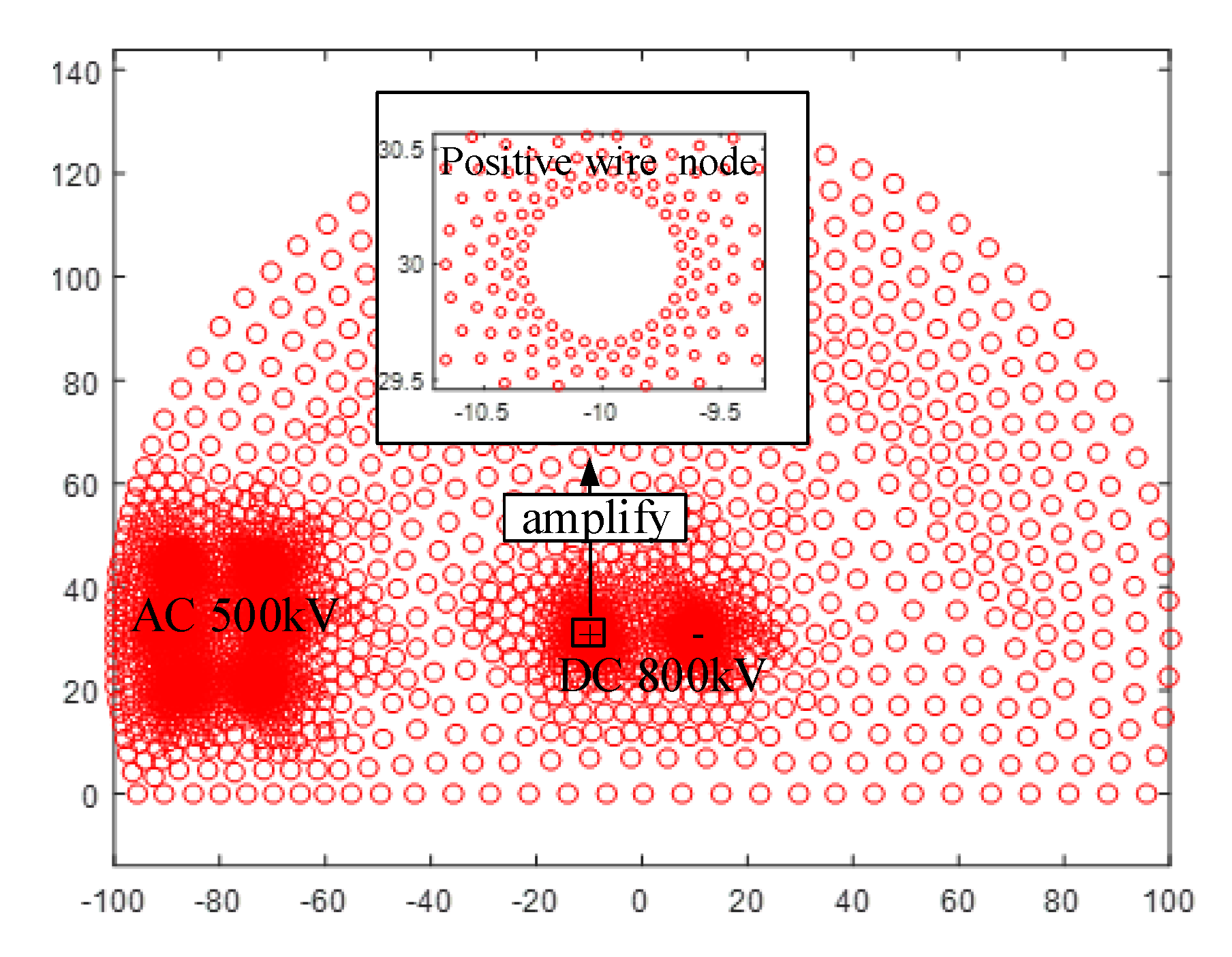
3. Calculation of Hybrid Ionized Field by the Meshless Local Petorv–Galerkin Method

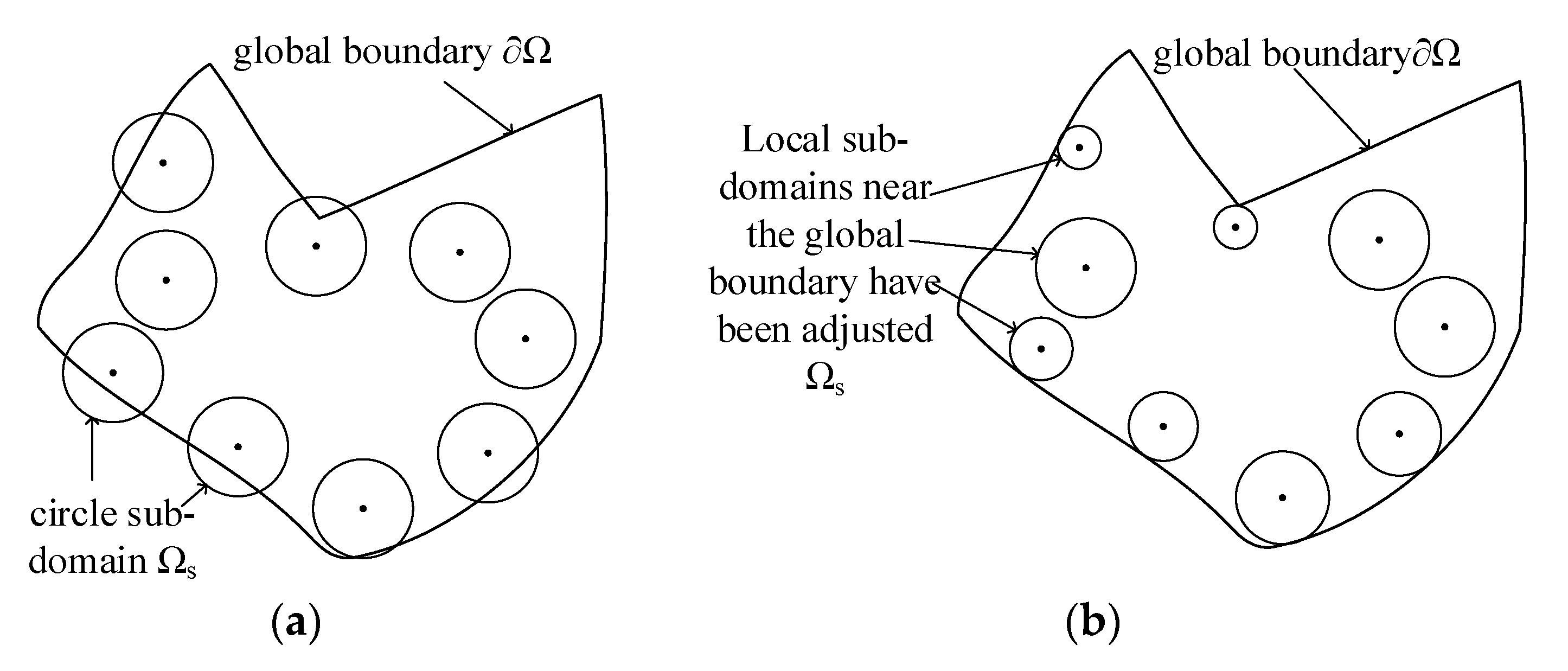
3.1. Shape Function

The interpolation function is constructed by RPIMp shape functions in the process of using the meshless method.

For an unknown field u(x), its interpolation function u^h(x) can be expressed as follows [17,18]:

$$u^h(x)={\displaystyle \sum _{i=1}^n{R}_i(x)a_i+}{\displaystyle \sum _{j=1}^m{p}_j(x)b_j=R^{\mathrm{T}}(x)a+P^{\mathrm{T}}(x)b}$$

(8)

In Equation (8), n is the number of nodes in the support domain. m is the number of terms of monomials. R^T is the vector of radial basis vector. P^T is the polynomial basis vector. a and b are unknown vectors. R^T, P^T, a, and b are defined as:

$$R^{\mathrm{T}}=\left[R_1\left(x\right),R_2\left(x\right),...,R_n\left(x\right)\right]$$

(8a)

$$p^{\mathrm{T}}=\left[p_1\left(x\right),p_2\left(x\right),...,p_m\left(x\right)\right]$$

(8b)

$$a=\left[a_1,a_2,...,a_n\right]$$

(8c)

$$b=\left[b_1,b_2,...,b_m\right]$$

(8d)

The unknown field represented by the fitting function is matched to the values of node n, which can be obtained as follows:

$$u=R_Q\left(x\right)a+p_m\left(x\right)b$$

(9)

where, $u=\left[u_1,u_2,\dots ,u_n\right]$ is the vector in node n; $R_Q={\left[R\left(x_1\right),R\left(x_2\right),\dots ,R\left(x_n\right)\right]}^{\mathrm{T}}$ is a n × n matrix containing radial basis function (RBF) vector; $p_{\mathrm{m}}=[p\left(x_1\right),p\left(x_2\right),...,p\left(x_m\right){]}^{\mathrm{T}}$ is a n × m polynomial matrix.

The shape function Φ(x) is defined as:

$$\Phi (x)=\left[R^{\mathrm{T}}(x)S_a+p^{\mathrm{T}}{S}_b\right]=\left[{\mathsf{\Phi }}_1(x),{\mathsf{\Phi }}_2(x),...,{\mathsf{\Phi }}_n(x)\right]$$

(10)

where

$$S_a=R_Q^{-1}-R_Q^{-1}{p}_m{S}_b$$

(11)

$$S_b={\left[p_m^T{R}_Q^{-1}{p}_m\right]}^{-1}{p}_m^{\mathrm{T}}{R}_Q^{-1}$$

(12)

One of the main advantages of the shape function built by RBFs is that it satisfies the Kronecker delta function property [19,20], which is:

$${\mathsf{\Phi }}_i(x=x_j)=\{\begin{array}{l}1i=j,j=1,2,...,n\\ 0i\ne j,i,j=1,2,...,n\end{array}$$

(13)

This important property enables the MLPG method to impose the boundary conditions directly by the RPIMp in this paper, while other meshless methods need additional techniques.

3.2. Solving Poisson’s Equation

Poisson’s equation and boundary conditions are as follows:

$${\nabla }^{2}u(x)=-\frac{\rho (x)}{\epsilon }x\in \mathsf{\Omega }$$

(14)

$$u(x)=u_0\mathrm{on}{\mathsf{\Gamma }}_u$$

(15)

$$\frac{\partial u(x)}{\partial n}=\overline{q}on{\mathsf{\Gamma }}_q$$

(16)

where the problem boundary is $\partial \mathsf{\Omega }={\mathsf{\Gamma }}_u\cup {\mathsf{\Gamma }}_q$ and n is the normal vector for the outer boundary.

The MLPG method is based on the local weak form, in which Equations (14)–(16) can be obtained by a weighted residual method:

$${\displaystyle {\int }_{{\mathsf{\Omega }}_s}\left({\nabla }^{2}u+\frac{\rho (x)}{\epsilon }\right)vd\mathsf{\Omega }}-\alpha {\displaystyle {\int }_{{\mathsf{\Gamma }}_{su}}\left(u-u_0\right)vd\mathsf{\Gamma }=0}$$

(17)

where u is trial function, v represents the test functions and α >> 1 is the penalty parameter. ${\mathsf{\Gamma }}_{su}$ is a part of the essential boundary. If the sub-domain has no intersection with the global essential boundary, the second part of Equation (17) vanishes [21].

In the MLPG method, the trial function and test function can be chosen from different function spaces. In this paper, the MLPG selects the Heaviside function as the test function, which is given in Equation (18) [22]:

$$v\left(x\right)=\{\begin{array}{l}1\mathrm{for}x\in {\mathsf{\Omega }}_s\\ 0\mathrm{for}x\notin {\mathsf{\Omega }}_s\end{array}$$

(18)

By using the Heaviside function, the local weak form of Poisson’s equation can be written as:

$${\displaystyle {\int }_{{\mathsf{\Omega }}_s}\frac{\rho \left(x\right)}{\epsilon }d\mathsf{\Omega }}+{\displaystyle {\int }_{L_s}\frac{\partial u}{\partial n}d\mathsf{\Gamma }}+{\displaystyle {\int }_{{\mathsf{\Gamma }}_{su}}\frac{\partial u}{\partial n}d\mathsf{\Gamma }}+{\displaystyle {\int }_{{\mathsf{\Gamma }}_{sq}}\overline{q}}d\mathsf{\Gamma }-\alpha {\displaystyle {\int }_{{\mathsf{\Gamma }}_{su}}\left(u-u_0\right)d\mathsf{\Gamma }}=0$$

(19)

where Γ_sq is the intersecting part of the local support domain and the charge boundary. If the local support domain has no intersection with the two boundary conditions, the integral is equal to zero.

In the conventional MLPG method, the unified size of the local sub-domain Ω_s is often used as the integral, as shown in Figure 1a. On the border and its vicinity, the local sub-domain Ω_s inevitably overlaps with the problem domain boundaries and boundary part. The process of implementation in the conventional MLPG method, according to the boundary of different shapes and different node locations, determines whether the local sub-domain Ω_s of each node is beyond the problem domain. This increases the difficulty of programming.

In order to simplify the MLPG method, the radius of local sub-domains was adjusted to the nodes close to the global boundary, but not exactly on the boundary. Therefore, the sub-domains for such nodes would not cross over the global boundary, as Figure 1b shows. The main idea of the technique can be found in Reference [23].

Through adaptive narrowing near the boundary nodes after local sub-domain Ω_s, the function Equation (19) for the sub-domains entirely within the problem domain can be simplified:

$${\displaystyle {\int }_{L_s}\frac{\partial u}{\partial n}d\mathsf{\Gamma }}=-{\displaystyle {\int }_{{\mathsf{\Omega }}_s}\frac{\rho \left(x\right)}{\epsilon }d\mathsf{\Omega }}$$

(20)

It can be seen that there is no domain integration involved in the left side of Equation (20). The boundary integrations are needed only over $L_s=\partial {\mathsf{\Omega }}_s$.

In the discrete equation, the nodes on the boundary use the RPIMp function to apply the boundary conditions. The system matrix can be obtained:

$$Ku=f$$

(21)

where $K_{ij}={\displaystyle {\int }_{L_s}\frac{\partial {\mathsf{\Phi }}_j}{\partial n}d\mathsf{\Gamma }}$ is for the internal nodes. $K_{ij}={\mathsf{\Phi }}_i^j$ is for the nodes on Γ_u. $K_{ij}=\frac{\partial {\mathsf{\Phi }}_i^j}{\partial n}$ is for the nodes on Γ_q. In addition, $f_i=-{\displaystyle {\int }_{{\mathsf{\Omega }}_s}\frac{\rho \left(x\right)}{\epsilon }d\mathsf{\Omega }}$ is for the nodes in the interior of ∂Ω; $f_i=u_0$ is the nodes on Γ_u; $f_i=\overline{q}$ is the nodes on Γ_q.

3.3. The Solution of the Charge Conservation Equation

The charge transfer, as well as the composite coupling of the charge conservation equation’s solution, is the most difficult part in solving the hybrid ionized field. In this paper, the space charge density is solved directly from the charge conservation equation, according to the current differential principle.

On the conductor surface and at every point in the space outside the area, because the charge produced by the DC lines at t_n moment has not yet arrived in t_n+1 moment, the change of space charge density is caused by the electric field under the movement of ion migration. Therefore, by solving the charge conservation equation, the space charge density of the t_n+1 moment can be obtained.

Combining Formulas (1)–(3), these equations can be obtained:

$$\frac{K^{+}}{{\epsilon }_0}{({\rho }^{+}(t))}^2+\left(R/e-K^{+}/{\epsilon }_0\right){\rho }^{-}(t){\rho }^{+}(t)+\nabla {\rho }^{+}(t)\cdot V^{+}+\frac{\partial {\rho }^{+}(t)}{\partial t}=0$$

(22)

$$\frac{K^{-}}{{\epsilon }_0}{({\rho }^{-}(t))}^2+\left(R/e-K^{-}/{\epsilon }_0\right){\rho }^{+}(t){\rho }^{-}(t)+\nabla {\rho }^{-}(t)\cdot V^{-}+\frac{\partial {\rho }^{-}(t)}{\partial t}=0$$

(23)

In the Formulas (22) and (23), V⁺ and V⁻ are the migration velocity vectors of positive and negative ions:

$$V^{+}=k^{+}(-\nabla \phi )+w$$

(24)

$$V^{-}=-k^{-}(-\nabla \phi )+w$$

(25)

Because the meshless method only requires node partitioning when constructing shape functions, it is very convenient to select the upstream node by controlling the size, as well as the position, of the local support domain. The selection of the upstream node is shown in Figure 2:

Assuming that the direction of the ion mobility velocity V_i is as shown in Figure 2, the upstream node can be determined by moving the normal support domain against the direction of the ion mobility velocity. Because the meshless method avoids the triangulation, it can avoid the judgment of the direction of the vector in the upper finite element when selecting the upstream node, and it is very convenient to use the size of the support domain to determine the number of the upstream nodes [23].

After the upstream node is determined, on the node i, the Formulas (22)–(25) can be described as follows:

$$\frac{\partial {\rho }_i{}^{+}(t)}{\partial t}=-\frac{K^{+}}{{\epsilon }_0}{({\rho }_i{}^{+}(t))}^2-\nabla {\rho }_i{}^{+}(t)\cdot V^{+}-\left(R/e-K^{+}/{\epsilon }_0\right){\rho }_i{}^{+}(t){\rho }_i{}^{-}(t)$$

(26)

$$\frac{\partial {\rho }_i{}^{-}(t)}{\partial t}=-\frac{K^{-}}{{\epsilon }_0}{({\rho }_i{}^{-}(t))}^2-\nabla {\rho }_i{}^{-}(t)\cdot V_i{}^{-}-\left(R/e-K^{-}/{\epsilon }_0\right){\rho }_i{}^{-}(t){\rho }_i{}^{+}(t)$$

(27)

$$V_i{}^{+}(t)=k^{+}(-\nabla {\phi }_i(t))+w(t)$$

(28)

$$V_i{}^{-}(t)=-k^{-}(-\nabla {\phi }_i(t))+w(t)$$

(29)

Using the notion of upstream node, the nodes i, j, k and i, l, n are the upstream nodes of the positive and negative charges, respectively. The potential gradient and charge density gradient of positive and negative charge at node i are respectively equal to the potential gradient and charge density gradient of the upstream support domain, and the first step is discrete in the upstream support domain.

At the time of t_n+1, the Formulas (26)–(27) can be expressed as:

$${\rho }_i{}^{+}(t_{\mathrm{n}+1})={\rho }_i{}^{+}(t_{\mathrm{n}})-\mathsf{\Delta }\mathrm{t}(\frac{K^{+}}{{\epsilon }_0}{({\rho }_i{}^{+}(t))}^2+\nabla {\rho }_{ijk}{}^{+}(t)\cdot V_i{}^{+}(t_{\mathrm{n}})+\left(R/e-K^{+}/{\epsilon }_0\right){\rho }_i{}^{+}(t_{\mathrm{n}}){\rho }_i{}^{-}(t))$$

(30)

$${\rho }_i{}^{-}(t_{n+1})={\rho }_i{}^{-}(t_n)-\mathsf{\Delta }t(\frac{K^{-}}{{\epsilon }_0}{({\rho }_i{}^{-}(t))}^2+\nabla {\rho }_{iln}{}^{-}(t)\cdot V_i{}^{-}(t_n)+\left(R/e-K^{-}/{\epsilon }_0\right){\rho }_i{}^{-}(t){\rho }_i{}^{+}(t))$$

(31)

In the local support domain of the MLPG method, the charge density can be expressed as:

$$\rho \left(x\right)={\displaystyle \sum _I^n{\mathsf{\Phi }}_I\left(x\right){\rho }_I}$$

(32)

where n is the number of nodes in the local support domain; ${\mathsf{\Phi }}_I\left(x\right)$ is RPIMp shape functions on the node i.

In local support domain, the solution process of positive and negative charge density is considered to be as follows:

$$\begin{array}{l}\nabla {\rho }_{ijk}{}^{+}(t)\cdot V_i{}^{+}(t_{\mathrm{n}})=\nabla \left({\displaystyle \sum _{I=i,j,k}^n{\mathsf{\Phi }}_I\left(x\right){\rho }_I{}^{+}(t)}\right)\cdot V_i{}^{+}(t_{\mathrm{n}})=\\ {\displaystyle \sum _{I=i,j,k}^n\left(\nabla ({\mathsf{\Phi }}_{I,x}\left(x\right){\rho }_I{}^{+}(t))\cdot {\mathrm{V}}_x{}^{+}(t_{\mathrm{n}})+\nabla ({\mathsf{\Phi }}_{I,y}\left(x\right){\rho }_I{}^{+}(t))\cdot {\mathrm{V}}_y{}^{+}(t_{\mathrm{n}})\right)}\end{array}$$

(33)

$$\begin{array}{l}\nabla {\rho }_{iln}{}^{-}(t)\cdot V_i{}^{-}(t_n)=\nabla \left({\displaystyle \sum _{I=i,l,n}^n{\mathsf{\Phi }}_I\left(x\right){\rho }_{I-}(t)}\right)\cdot V_i{}^{-}(t_n)=\\ {\displaystyle \sum _{I=i,l,n}^n\left(\nabla ({\mathsf{\Phi }}_{I,}{}_x\left(x\right){\rho }_I{}^{-}(t))\cdot {\mathrm{V}}_x{}^{-}(t_n)+\nabla ({\mathsf{\Phi }}_{I,y}\left(x\right){\rho }_I{}^{-}(t))\cdot {\mathrm{V}}_y{}^{-}(t_n)\right)}\end{array}$$

(34)

The choice of the time-step $\mathsf{\Delta }t$ must take into account the balance between the accuracy and the stability of the time plan. Therefore, the following definition is used:

$$\mathsf{\Delta }t=\frac{2C}{3}\min \mathsf{\Delta }r\times \min (r_D)$$

(35)

where $r_D$ is the radius of the inscribed circle of support domain; C is of order 1; $\mathsf{\Delta }r$ reflects the spacing between nodes, using the distance between Gauss quadrature points.

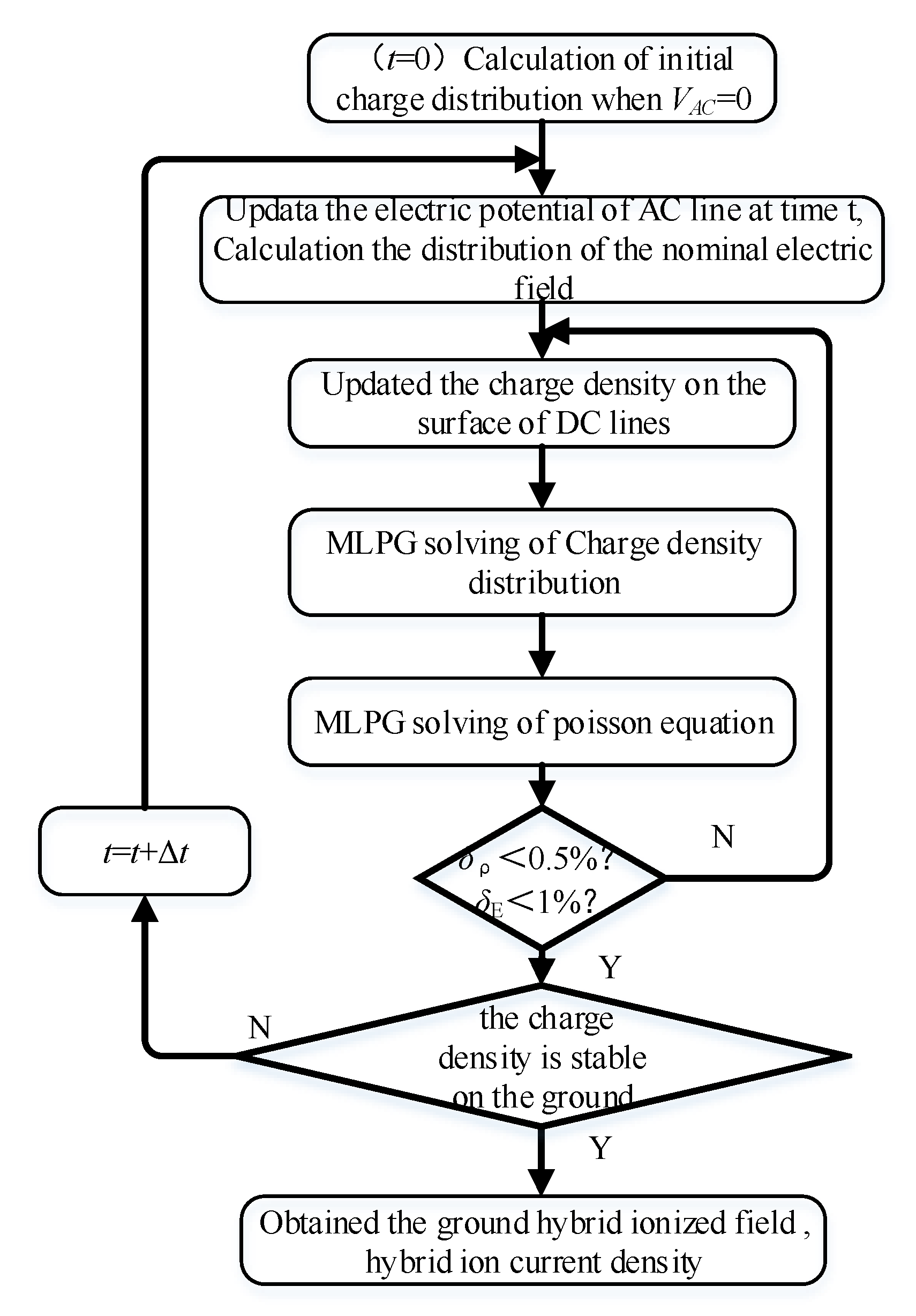
3.4. Calculation Process

Based on the MLPG method, the calculation process described in this paper is shown in Figure 3. As Figure 3 shows, the calculation of the hybrid ionized field is carried out in the time domain. In order to accelerate the convergence of the algorithm, the space charge density of the DC wire is calculated as the initial charge density of the hybrid electric field. In the process of calculation, every parameter is determined under normal weather, including the starting corona electric field, ion mobility, etc.

The surface charge density of the conductor is determined iteratively, so the surface gradient of the conductor is equal to the corona onset initial gradient (Kaptzov’s assumption). The updated formula for DC charge density on the surface of the conductor is expressed as follows [24]:

$${\rho }_i(t_{n+1})={\rho }_i(t_n)\left[1+\mu \left(E_{\max }(t_n)-E_c\right)/\left(E_{\max }(t_n)+E_c\right)\right]$$

(36)

where ${\rho }_i(t_{n+1})$ and ${\rho }_i(t_n)$ are the values of the surface space charge density of the wire surface in t_n+1 and t_n respectively. μ is the correction coefficient. In this paper, μ is 0.6; $E_{\max }(t_n)$ is the maximum electric field in t_n; E_c is starting corona electric field on the surface of the DC wire.

Because the hybrid ionized field is a time-varying coupling field, in the process of calculation, there are outer time-step loop and the inner charge density update loop. In the inner charge density update loop, when the error limit is met, which is calculated by Equations (37) and (38), it goes into the outer loop. In the outer time-step loop, the procedure is repeated until similar calculation results have been obtained during the last two cycles.

$${\delta }_{\rho }=\left|{\rho }_n(t_n)-{\rho }_{n-1}(t_n)\right|/{\rho }_{n-1}(t_n)$$

(37)

$${\delta }_E=\left|E_{\max }-E_c\right|/E_c$$

(38)

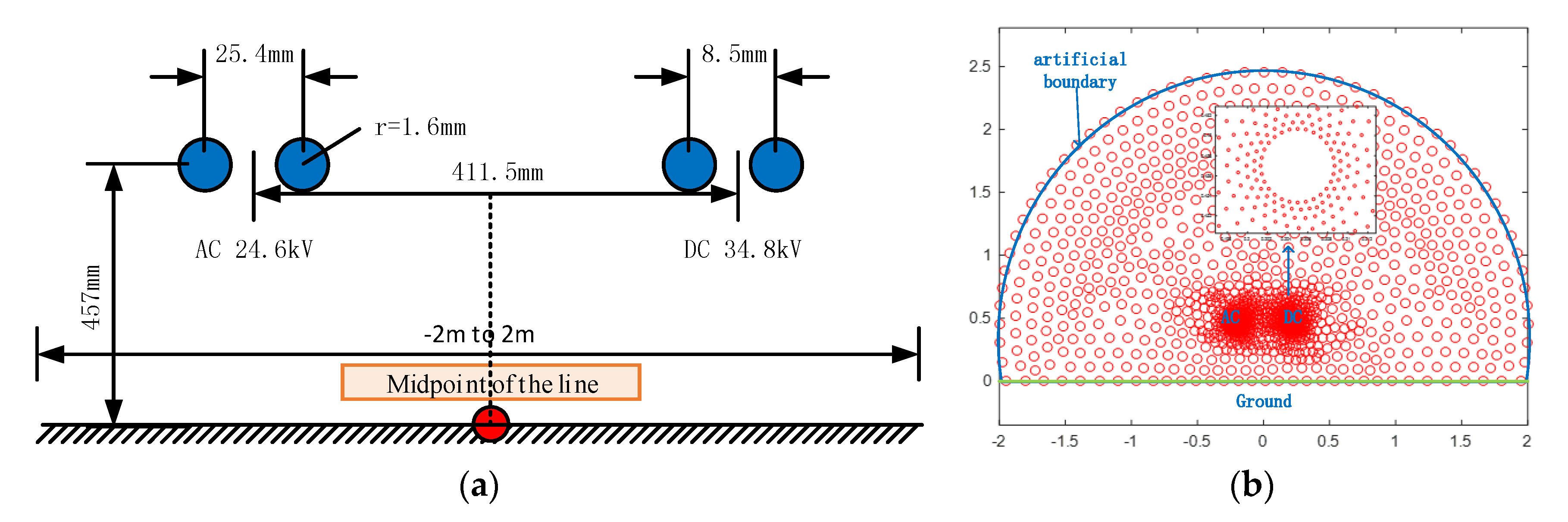
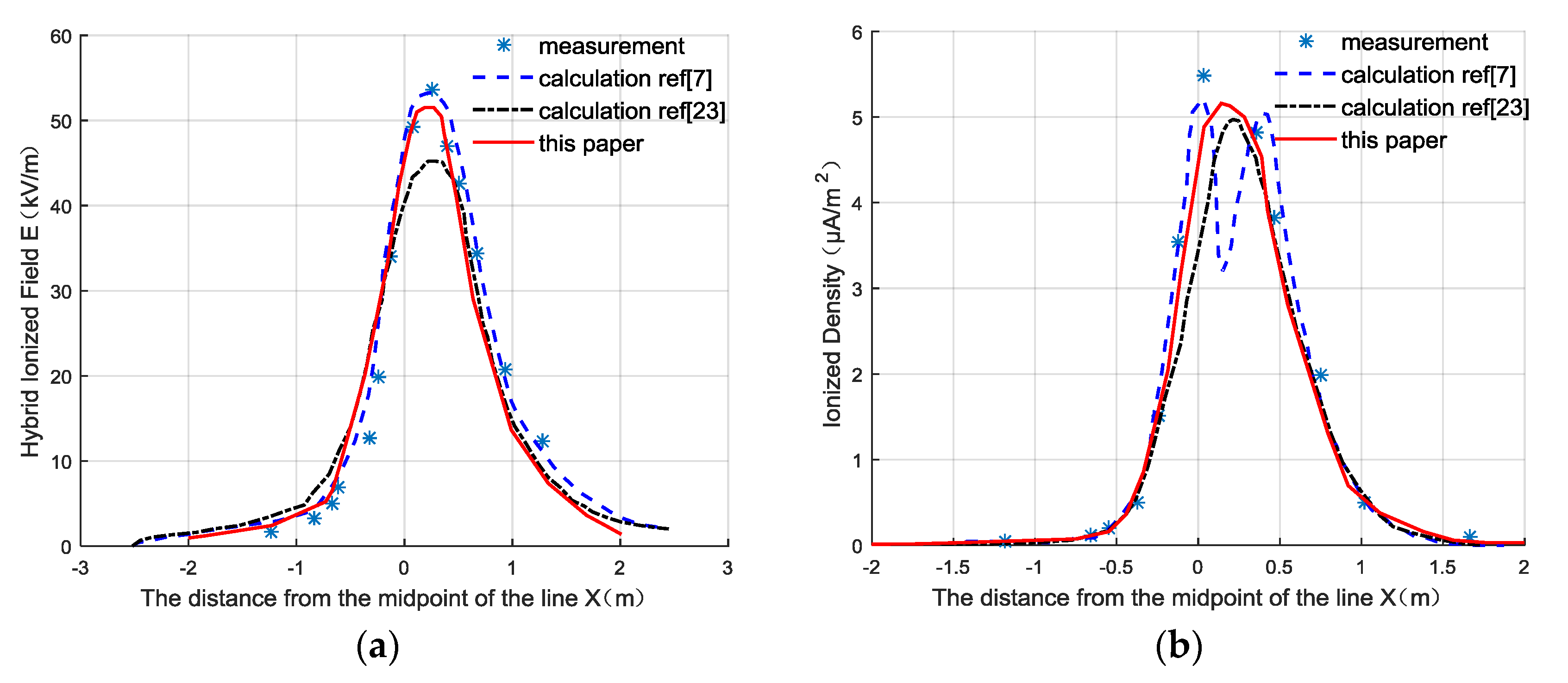
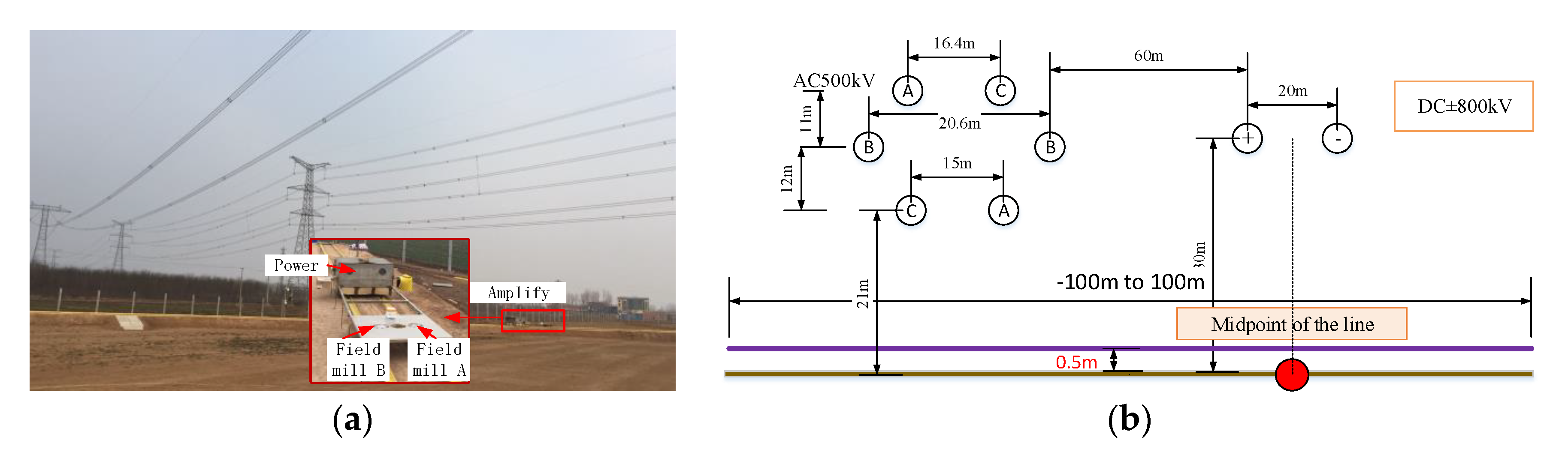
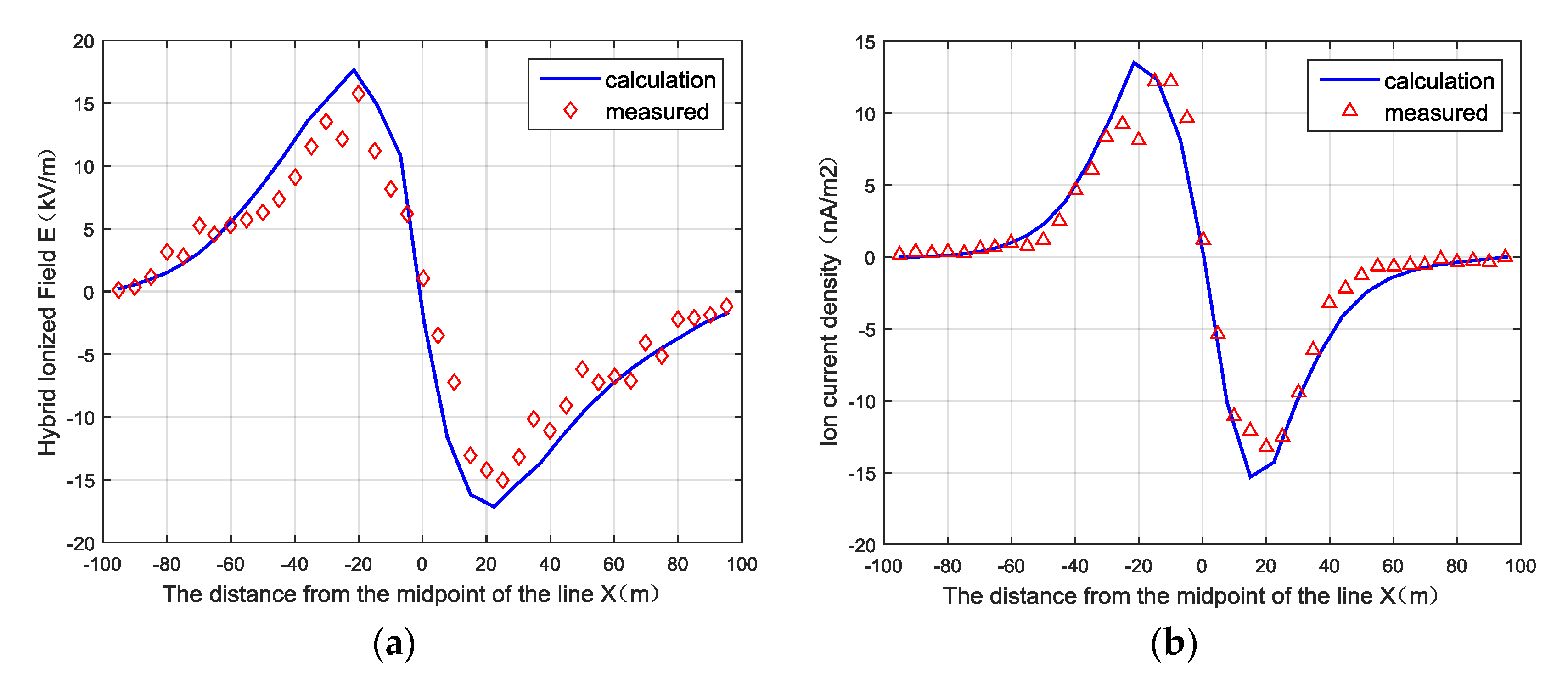
4. Validation Case

To verify the method proposed in this paper, the calculation results are compared with Reference [7,25]. The AC/DC hybrid line reduced-scale model is shown in Figure 4, and the split wire is equivalent to the wire with the equivalent radius. The hybrid ionized field and ion current density at ground level are calculated by the method proposed in this paper. The comparison results are shown in Figure 5a,b.

As shown in Figure 5, the calculation in this paper shows good consistency between the calculated results and the measured values, which verifies the validity of the algorithm and the calculation procedure.

In addition, the field distribution of the parallel line at about ±800 kV DC/500 kV AC has been studied. The field experiment and the wire structure are shown in Figure 6.

As shown in Figure 6a, the field experiment of hybrid ionized field can be carried out continuously. As shown in Figure 6b, the test position is 0.5 m from the ground. The measuring track is perpendicular to the line, and the length is 200 m. Set one measuring point per 5 m. The measurement data of each measuring point is obtained by the residence time of 30 s at each measurement point.

To reduce the error, the normal weather of the test data was chosen to verify the calculation results, and the measured value of field mills A and B were averaged. The calculation node of the MLPG is shown in Figure 7. The calculated and measured results of the hybrid ionized field and ion current density at the ground level are shown in Figure 8, showing good consistency between the calculated results and the measured values.

From what has been discussed above, this method can effectively predict the distribution of hybrid ionized field in AC/DC parallel lines.

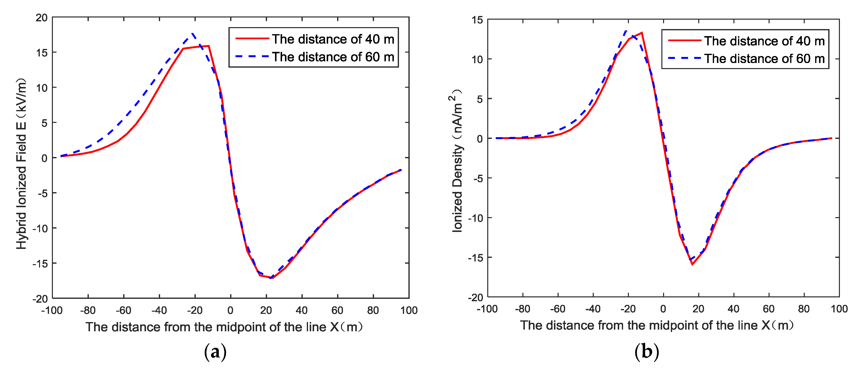
5. Applications

(1) The influence of the approach distance of AC transmission line

To confirm the influence of the approach distance to the hybrid ionized field in the transmission line, we used the line parameters in Figure 6 to calculate the hybrid ionized field and the distribution of the ion current density, which only change the approach distance from 60 to 40 m. The result of the calculation is shown in Figure 9 and

Table 1. The value and growth rate of calculation results when the approach distance is changed.

Approach Distance	Hybrid Ionized Field				Ion Current Density
	Maxk V/m	Growth Rate	Average kV/m	Growth Rate	Max nA/m2	Growth Rate	Average nA/m2	Growth Rate
60 m	17.64	0	−0.185	0	13.52	0	−0.205	0
40 m	15.9	−9.86%	−0.253	−36.7%	13.12	−2.96%	−0.245	−19.5%

. When the distance became shorter, the maximum values of the ionized field and ion current density were reduced by 9.86% and 2.96% respectively. The average values of the ionized field and ion current density were reduced by 36.7% and 19.5% respectively. The main reason for this is that when the distance is shorter, the influence of the AC electric field on the space flow motion of the ion is greater. Because of the shielding effect of AC lines, the ground ionized field is reduced.

(2) The influence of the AC transmission line’s voltage

To study the effect of AC voltage upon the hybrid ionized field, we used the line parameters in Figure 6 to calculate the hybrid ionized field and the distribution of the ion current density while only changing the division number and voltage grade of the AC lines. The hybrid ionized field were calculated when the voltage of the AC lines was 220 kV, 500 kV and 750 kV, respectively. The calculated result is shown in Figure 10 and

Table 2. The value and growth rate of calculation results when the AC voltage is changed.

AC Transmission Line Voltage	Hybrid Ionized Field				Ion Current Density
	Max kV/m	Growth Rate	Average kV/m	Growth Rate	Max nA/m2	Growth Rate	Average nA/m2	Growth Rate
220 kV	17.61	−0.17%	−0.168	9.1%	13.81	2.1%	−0.184	11.4%
500 kV	17.64	0	−0.185	0	13.52	0	−0.205	0
750 kV	17.12	−2.9%	−0.198	−7.02%	12.42	−8.13%	−0.223	−8.78%

. With increasing AC voltage, the hybrid ionized field and ion current density on the ground decreased. When the voltage of the AC lines changed from 220 to 500 kV, the maximum ionized field and ion current density were reduced by −0.17% and 2.1%, respectively. The average values of the ionized field and ion current density were reduced by 9.1% and 11.4%, respectively. When the voltage of the AC lines changed from 500 to 750 kV, the maximum values of the ionized field and ion current density were reduced by 2.9% and 8.1%, respectively. The average values of the ionized field and ion current density were reduced by 7.02% and 8.78%, respectively. The reason for this is that with the increase in the AC electric field, the motion disturbance of the space charge is enhanced, making the distribution of space charge under the line more dispersed.

When the AC/DC is parallel, the effect of DC voltage on the calculation results is similar to that when the DC line runs separately. There is some literature that has studied this, and specific effects can be found in Ref. [11]. Thus, this article does not research this any further.

6. Conclusions

In the above paper, an algorithm based on the MLPG method was proposed to calculate the hybrid ionized field of AC/DC parallel lines. The advantages of the calculation method are high accuracy and fast computing speed. The hybrid ionized field can be calculated in the time domain. At the same time, the ground hybrid ionized field of an 800 kV DC and 500 kV double AC parallel transmission line was measured and calculated. The accuracy of the algorithm and the influence of different parallel spacing and AC voltage level on the hybrid ionized field were analyzed. The main conclusions are as follows:

(1)

The MLPG method can be used to calculate the hybrid ionized field in time domain, and it can be seen from the comparison between measurement results and calculation results that the calculation method has high precision.

(2)

The existence of the AC line affects the space ion distribution. The shielding effect of the AC lines can reduce the hybrid ionized field near the AC side.

(3)

It can be seen that the calculation results related to the voltage level and parallel distance of AC lines. Appropriately reducing the parallel distance and increasing the AC voltage of the line can reduce the hybrid ionized field under the line.

References

- Maruvada, P.; Drogi, S. Field and ion interactions of hybrid AC/DC transmission lines. IEEE Trans. Power Deliv. 1988, 3, 1165–1172. [Google Scholar] [CrossRef]
- Clairmont, B.; Johnson, G.; Zaffanella, L.; Zelingher, S. The effect of HVAC-HVDC line separation in a hybrid corridor. IEEE Trans. Power Deliv. 1989, 4, 1338–1350. [Google Scholar] [CrossRef]
- Yin, H.; He, J.; Zhang, B.; Zeng, R. Finite Volume-Based Approach for the Hybrid Ion-Flow Field of UHVAC and UHVDC Transmission Lines in Parallel. IEEE Trans. Power Deliv. 2011, 26, 2809–2820. [Google Scholar] [CrossRef]
- Zhou, X.; Cui, X.; Lu, T.; Zhen, Y.; Luo, Z. A Time-Efficient Method for the Simulation of Ion Flow Field of the AC-DC Hybrid Transmission Lines. IEEE Trans. Magn. 2012, 48, 731–734. [Google Scholar] [CrossRef]
- Yang, Y.; Lu, J.; Lei, Y. A Calculation Method for the Hybrid Electric Field under UHVAC and UHVDC Transmission Lines in the Same Corridor. IEEE Trans. Power Deliv. 2010, 25, 1146–1153. [Google Scholar] [CrossRef]
- Li, W.; Zhang, B.; He, J.; Zeng, R. Calculation of the ion flow field of AC-DC hybrid transmission lines. IET Gener. Transm. Distrib. 2009, 3, 911–918. [Google Scholar] [CrossRef]
- Tian, Y.; Huang, X.; Tian, W.; Zhu, Y.; Zhao, L. Study on the hybrid ion-flow field of HVDC and HVAC transmission lines by the nodal discontinuous Galerkin time-domain method. Gener. Transm. Distrib. 2017, 11, 209–217. [Google Scholar] [CrossRef]
- Guillod, T.; Pfeiffer, M.; Franck, C.M. Improved Coupled Ion-Flow Field Calculation Method for AC/DC Hybrid Overhead Power Lines. IEEE Trans. Power Deliv. 2014, 29, 2493–2501. [Google Scholar] [CrossRef] [Green Version]
- Straumann, U.; Franck, C.M. Ion-Flow Field Calculations of AC/DC Hybrid Transmission Lines. IEEE Trans. Power Deliv. 2013, 28, 294–302. [Google Scholar] [CrossRef] [Green Version]
- Ji, Q.; Zou, J.; Zhang, J.; Lu, Y.; Lee, J. Space-Time Pattern of Ion Flow Under AC/DC Hybrid Overhead Lines and Its Application. IEEE Trans. Power Deliv. 2017. [Google Scholar] [CrossRef]
- Zhou, X.; Cui, X.; Lu, T.; Liu, Y.; Li, X.; He, J.; Bai, R.; Zhen, Y. Shielding Effect of HVAC Transmission Lines on the Ion-Flow Field of HVDC Transmission Lines. IEEE Trans. Power Deliv. 2013, 28, 1094–1102. [Google Scholar] [CrossRef]
- Xiao, F.; Zhang, B.; Mo, J.; He, J. Calculation of 3-D Ion Flow Field at the Crossing of HVDC Transmission Lines by Method of Characteristics. IEEE Trans. Power Deliv. 2017. [Google Scholar] [CrossRef]
- Zhou, X. Physical Spline Finite Element (PSFEM) Solutions to One Dimensional Electromagnetic Problems. Prog. Electromagn. Res. 2003, 40, 271–294. [Google Scholar] [CrossRef] [Green Version]
- Li, J.; Lu, X.; Farquharson, C. A finite-element time-domain forward solver for electromagnetic methods with a complex-shape transmitting loop. SEG Tech. Program Expand. 2017, 1152–1157. [Google Scholar] [CrossRef]
- Zhang, B.; Mo, J.; He, J.; Zhuang, C. A Time-Domain Approach of Ion Flow Field around AC–DC Hybrid Transmission Lines Based on Method of Characteristics. IEEE Trans. Magn. 2016, 52, 1–4. [Google Scholar] [CrossRef]
- Tian, Y.; Huang, X.; Tian, W. Hybrid method for calculation of ion-flow fields of HVDC transmission lines. IEEE Trans. Dielectr. Electr. Insul. 2016, 23, 2830–2839. [Google Scholar] [CrossRef]
- Benbouza, N.; Louai, F.Z.; Feliachi, M.; Zaoui, A. Electromagnetic Field Computation in Linear Electromagnetic Actuators Using the Meshless Local Petrov Galerkin Method. Acta Electrotech. Inform. 2016, 16, 27–31. [Google Scholar] [CrossRef]
- Liu, F.; Su, D.; Zhang, Y. A 3-D Unconditionally Stable Laguerre-Rpim Meshless Method for Time-Domain Electromagnetic Computations. Prog. Electromagn. Res. M 2013, 31, 279–293. [Google Scholar] [CrossRef]
- Lai, S.; Wang, B.; Duan, Y. Solving Helmholtz Equation by Meshless Radial Basis Functions Method. Prog. Electromagn. Res. B 2010, 24, 351–367. [Google Scholar] [CrossRef]
- Li, Q. Application of meshless local Petrov-Galerkin (MLPG) to problems with singularities, and material discontinuities, in 3-D elasticity. Comput. Model. Eng. Sci. 2003, 13, 571–585. [Google Scholar]
- Yuan, X.; Gu, G.; Zhao, M. Application of Meshless Local Petrov–Galerkin Method in Inhomogeneous Electromagnetic Field. In Proceedings of the International Conference on Electrical Engineering and Automation Control, Nanjing, China, 21–23 April 2017. [Google Scholar]
- Fonseca, A.; Corrêa, B.; Silva, E. Improving the mixed formulation for meshless local Petrov-Galerkin method. IEEE Trans. Magn. 2010, 46, 2907–2910. [Google Scholar] [CrossRef]
- Liu, G.; Gu, Y. An Introduction to Meshfree Methods and Their Programming; Springer: Dordrecht, The Netherlands, 2005. [Google Scholar]
- Wang, Z.; Lu, T.; Li, X. Predictive analysis of ion flow field at the ground level under HVAC and HVDC hybrid transmission lines. In Proceedings of the 2014 IEEE Conference on Electrical Insulation and Dielectric Phenomena, Des Moines, IA, USA, 19–22 October 2014; pp. 526–529. [Google Scholar]
- Zhao, T.; Illan, J.; Cohol, J.M.; Hinton, R.D.; Sebo, S.A.; Kasten, D.G. Design, construction and utilization of a new reduced-scale model for the study of hybrid (AC and DC) line corona. In Proceedings of the IEEE Power Engineering Society, Transmission and Distribution Conference, Chicago, IL, USA, 10–15 April 1994; pp. 239–245. [Google Scholar]