A Transient Productivity Model of Fractured Wells in Shale Reservoirs Based on the Succession Pseudo-Steady State Method

Abstract
:1. Introduction
2. Physical Model and Basic Assumptions
- (1)
- The model is for isothermal single-phase shale gas flow, and vertical flow is neglected.
- (2)
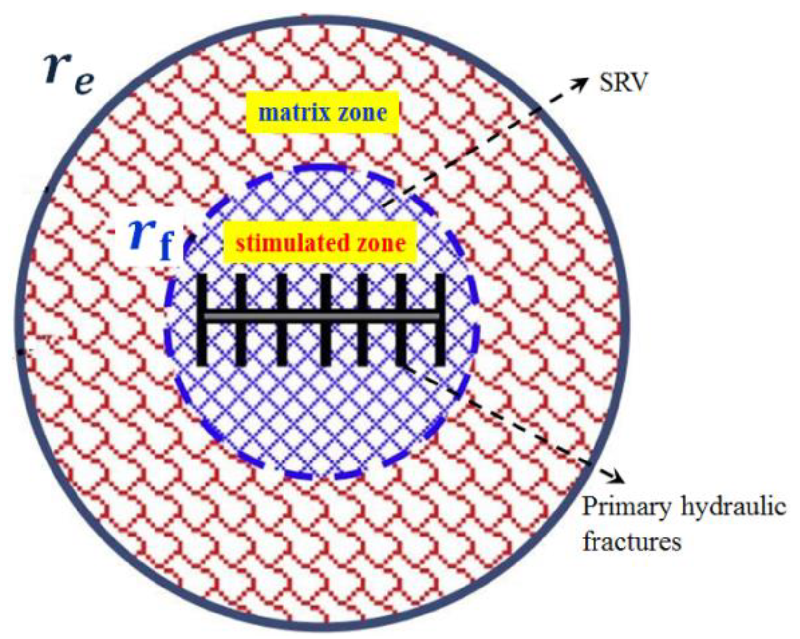
- The reservoir is composite with the matrix zone and stimulated zone, and the reservoir has a constant and uniformed thickness with the upper and lower boundaries closed.
- (3)
- The gas seepage is characterized by Kundsen number in matrix zone with the radius of while the gas flow is consistent with Darcy law in stimulated zone with the radius of .
3. Mathematical Model
3.1. Steady-State Productivity Model
3.1.1. Shale Matrix Gas Seepage Model
3.1.2. Stimulated Region Gas Seepage Model
3.1.3. Steady-State Productivity Model
3.2. Unsteady-State Productivity Model
3.2.1. The Solution of Initial Production
3.2.2. The Solution of Production at the Next Production Time Step
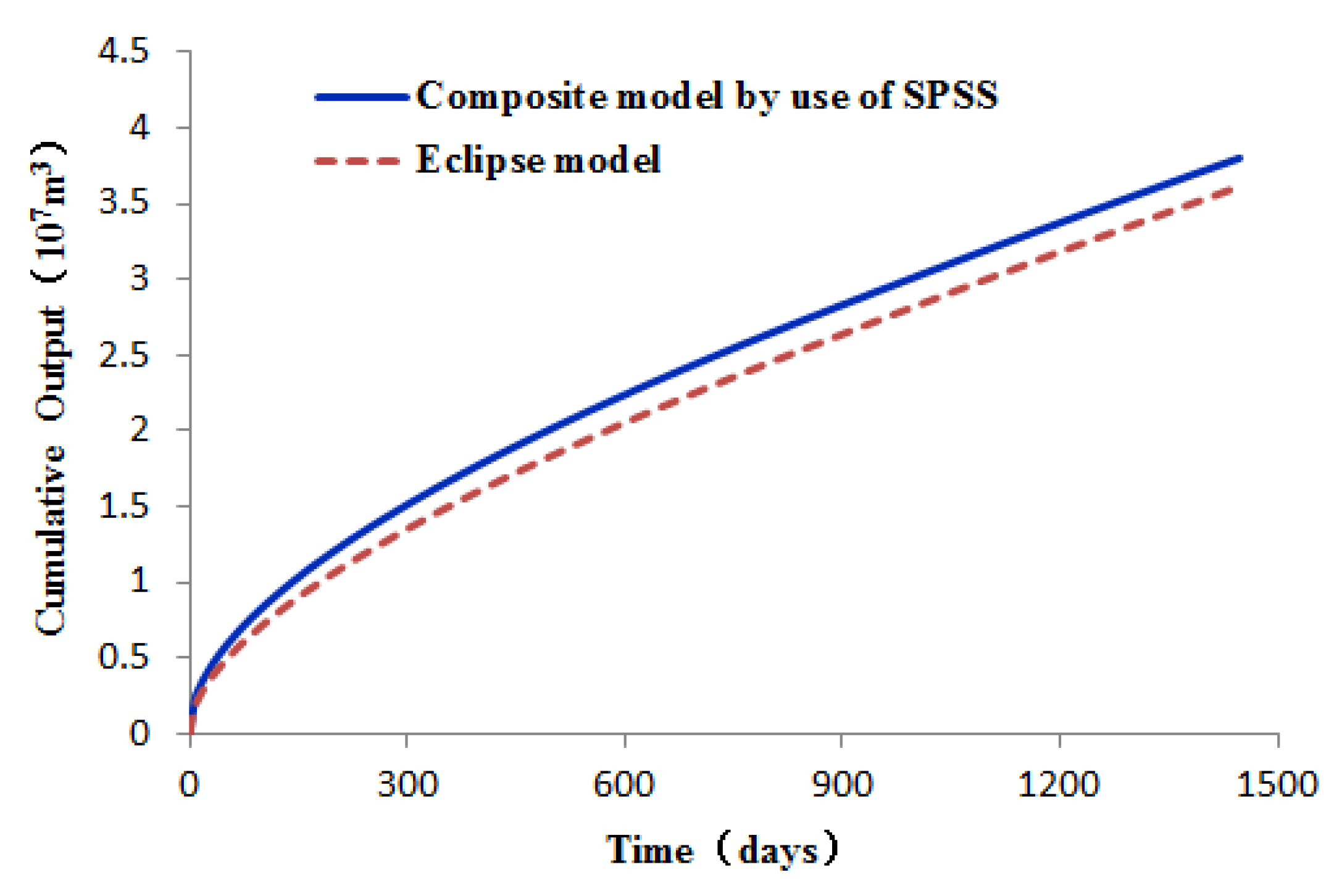
3.3. Model Validation
4. Results and Discussion
5. Conclusions
- (1)
- The productivity prediction model based on the SPSS method provides a theoretical basis for the transient productivity calculation of shale fractured horizontal wells, and it has the characteristics of simple solution process, fast computation speed and high agreement with numerical simulation results.
- (2)
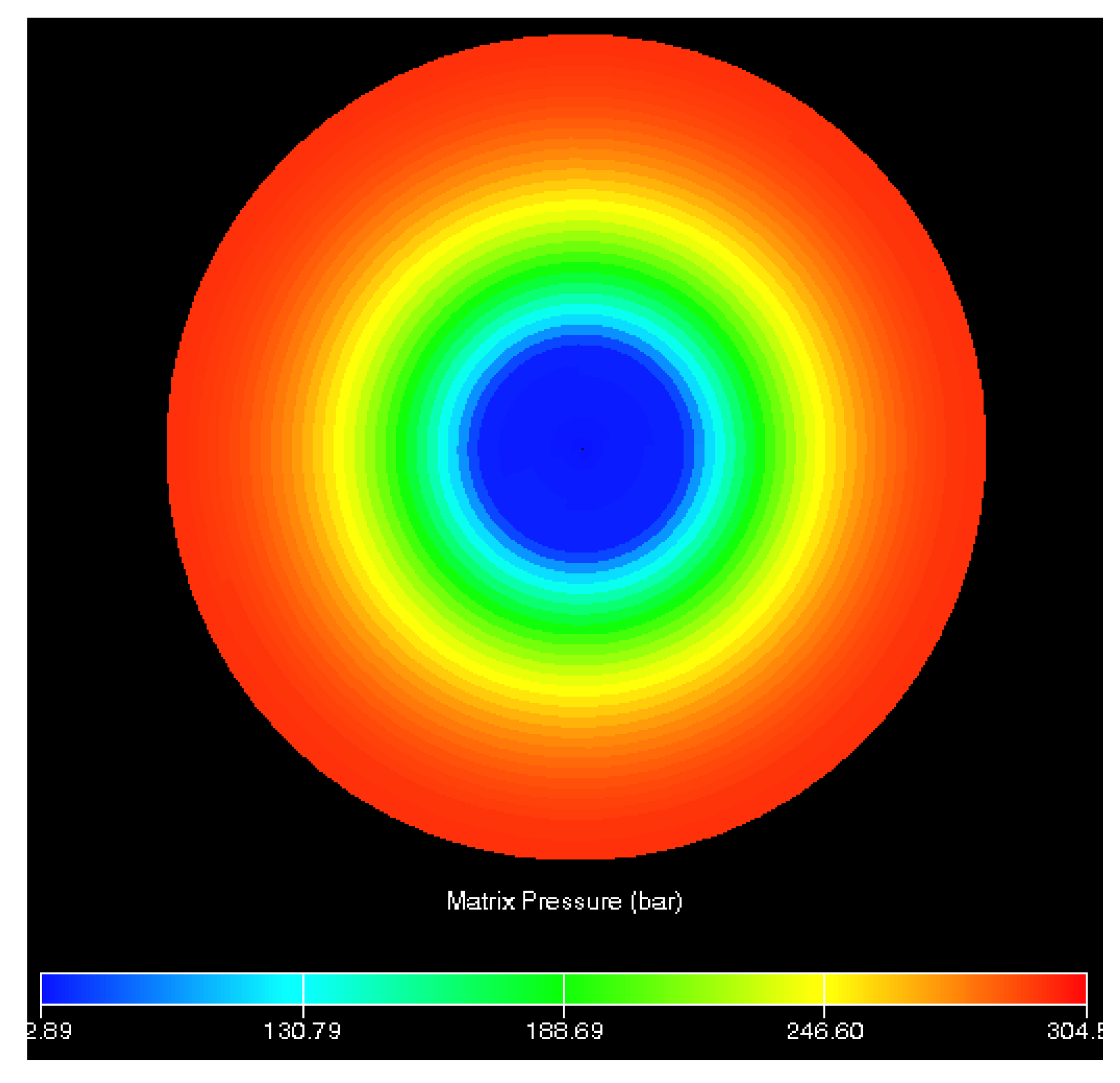
- The pressure wave propagates from the bottom of the well to the outer boundary of the volume fracturing zone, and then propagates from the outer boundary of the fracturing zone to the reservoir boundary.
- (3)
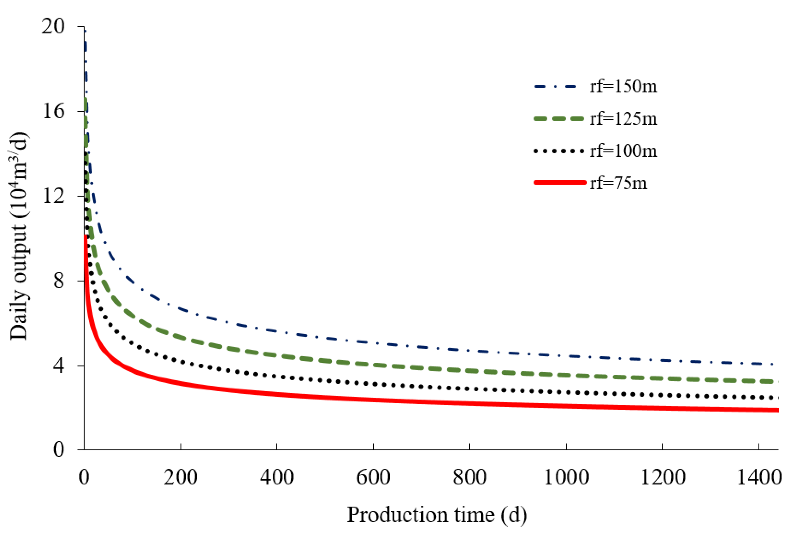
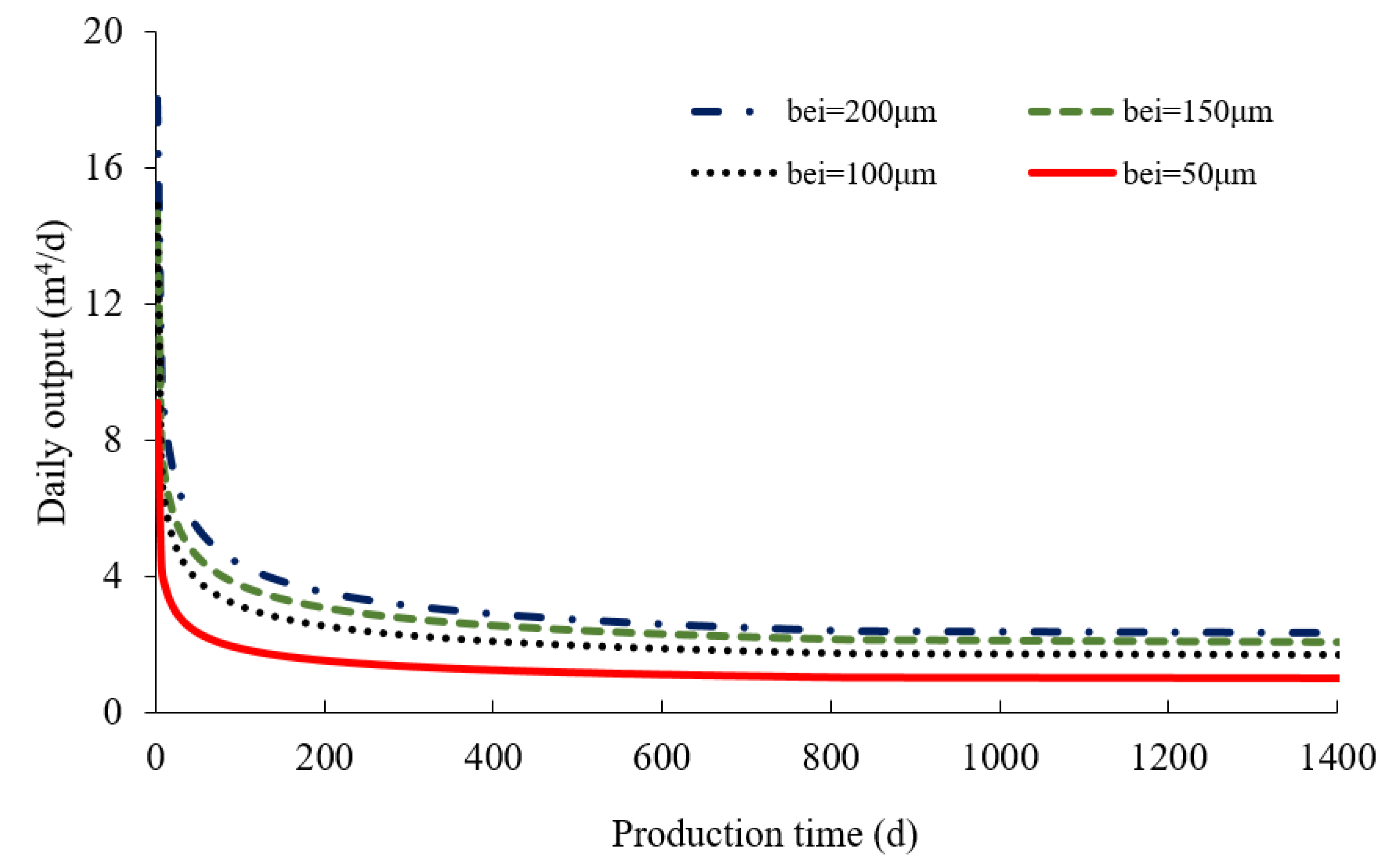
- With the increase of fracturing zone radius, the initial average aperture of fractures, maximum fracture length, the productivity of shale gas increases, and the increase rate gradually decreases. When the fracturing zone radius is 150 m, the daily output is approximately twice as much as that of 75 m. If the initial average aperture of fractures is 50 μm, the daily output is about half of that when the initial average aperture is 100 μm. When the maximum fracture length increases from 50 m to 100 m, the daily output only increases about by 25%.
- (4)
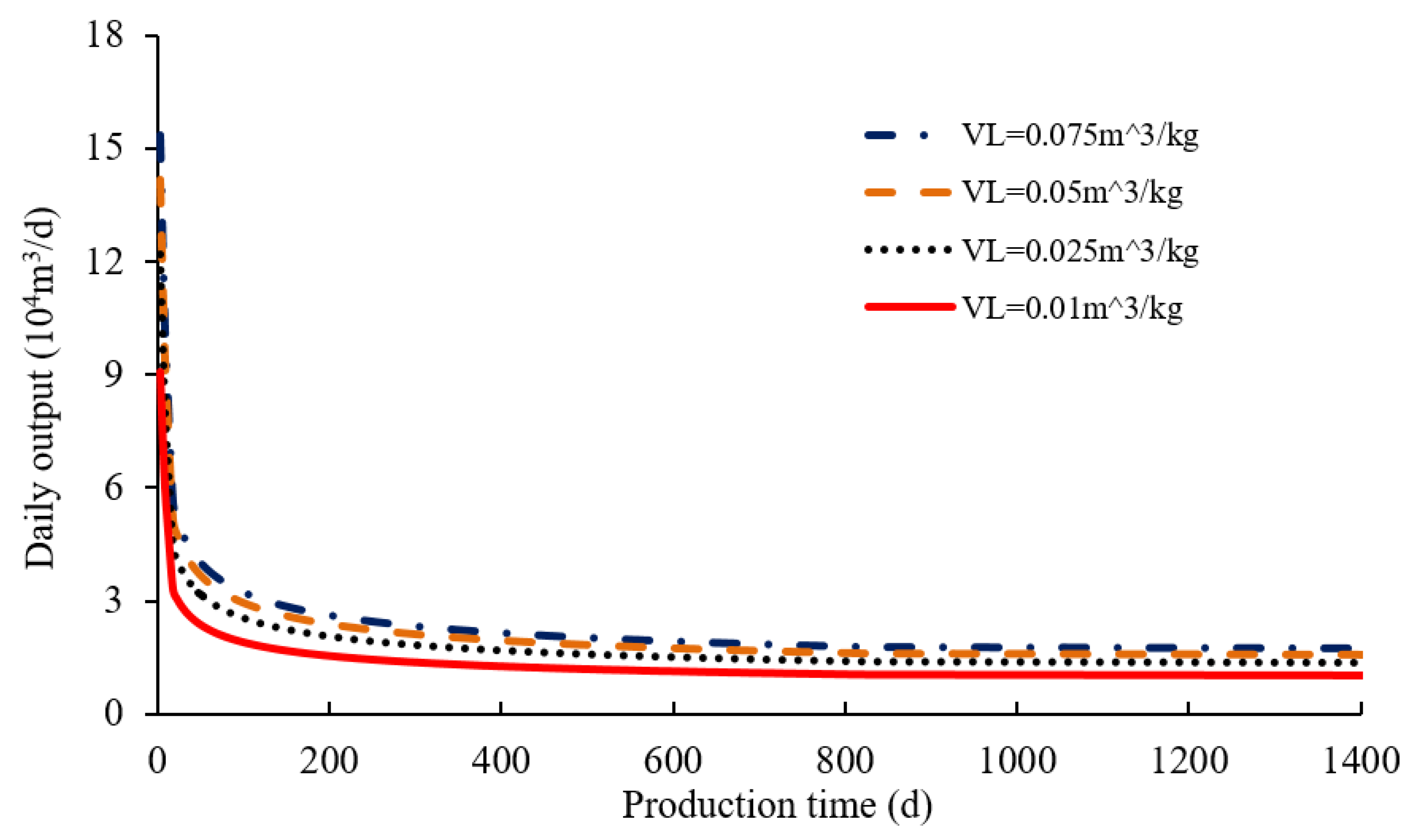
- When the Langmuir volume is relatively large, the daily outputs of different Langmuir volumes are almost identical, and the effect of Langmuir volume on the desorption output can almost be ignored.
Author Contributions
Funding
Acknowledgments
Suggestion
Conflicts of Interest
References
- Li, J.; Chen, Z.; Wu, K.; Li, R.; Xu, J.; Liu, Q.; Qu, S.; Li, X. Effect of water saturation on gas slippage in tight rocks. Fuel 2018, 225, 519–532. [Google Scholar] [CrossRef]
- Dejam, M.; Hassanzadeh, H.; Chen, Z. Pre-Darcy Flow in Porous Media. Water Resour. Res. 2017, 53, 8187–8210. [Google Scholar] [CrossRef]
- Ziarani, A.S.; Aguilera, R. Knudsen’s permeability correction for tight porous media. Tran. Porous Media 2012, 91, 239–260. [Google Scholar]
- Zou, C.; Dong, D.; Wang, S.; Li, J.; Li, X.; Wang, Y.; Li, D.; Cheng, K. Geological characteristics and resource potential of shale gas in China. Petroleum Explor. Dev. Online 2010, 37, 641–653. [Google Scholar] [CrossRef]
- Zuo, C.; Chengjin, X.; Tingxue, J.; Yuming, Q. Proposals for the application of fracturing by stimulated reservoir volume (SRV) in shale gas wells in China. Nat. Gas Ind. 2010, 30, 30–32. [Google Scholar]
- Rui, Z.; Wang, X.; Zhang, Z.; Lu, J.; Chen, G.; Zhou, X.; Patil, S. A realistic and integrated model for evaluating oil sands development with steam assisted gravity drainage technology in Canada. Appl. Energy 2018, 213, 76–91. [Google Scholar]
- Wu, K.; Chen, Z.; Li, X.; Dong, X. Methane storage in nanoporous material at supercritical temperature over a wide range of pressures. Sci. Rep. 2016, 6, 33–46. [Google Scholar] [CrossRef] [PubMed]
- Dejam, M.; Hassanzadeh, H. Diffusive leakage of brine from aquifers during CO2 geological storage. Adv. Water Resour. 2018, 111, 36–57. [Google Scholar] [CrossRef]
- Rui, Z.; Cui, K.; Wang, X.; Chun, J.; Li, Y.; Zhang, Z.; Lu, J.; Chen, G.; Zhou, X.; Patil, S. A comprehensive investigation on performance of oil and gas development in Nigeria: Technical and non-technical analyses. Energy 2018, 158, 666–680. [Google Scholar] [CrossRef]
- Clarkson, C.R. Production data analysis of unconventional gas wells: review of theory and best practices. Int. J. Coal Geol. 2013, 109, 101–146. [Google Scholar] [CrossRef]
- Zeng, F.; Cheng, X.; Guo, J.; Chen, Z.; Xiang, J. Investigation of the initiation pressure and fracture geometry of fractured deviated wells. J. Petroleum Sci. Eng. 2018, 165, 412–427. [Google Scholar] [CrossRef]
- Deng, J.; Zhu, W.; Ma, Q. A new seepage model for shale gas reservoir and productivity analysis of fractured well. Fuel 2014, 124, 232–240. [Google Scholar] [CrossRef]
- Zeng, F.; Guo, J.; Ma, S.; Chen, Z. 3D observations of the hydraulic fracturing process for a model non-cemented horizontal well under true triaxial conditions using an X-ray CT imaging technique. J. Petroleum Sci. Eng. 2018, 52, 128–140. [Google Scholar] [CrossRef]
- Gao, S.; Liu, H.; Ye, L.; Hu, Z.; Chang, J.; An, W. A coupling model for gas diffusion and seepage in SRV section of shale gas reservoirs. Nat. Gas Ind. B 2017, 4, 120–126. [Google Scholar] [CrossRef]
- Zeng, F.H.; Guo, J.C. Optimized design and use of induced complex fractures in horizontal wellbores of tight gas reservoirs. Rock Mech. Rock Eng. 2016, 49, 1411–1423. [Google Scholar] [CrossRef]
- Loucks, R.G.; Reed, R.M.; Ruppel, S.C.; Jarvie, D.M. Morphology, genesis, and distribution of nanometer-scale pores in siliceous mudstones of the Mississippian Barnett Shale. J. Sediment. Res. 2009, 79, 848–861. [Google Scholar] [CrossRef]
- Wendong, W.; Yuliang, S.; Qi, Z.; Gang, X.; Shiming, C. Performance-based Fractal Fracture Model for Complex Fracture Network Simulation. Petroleum Sci. 2018, 1, 1–9. [Google Scholar]
- Rui, Z.; Cui, K.; Wang, X.; Lu, J.; Chen, G.; Ling, K.; Patil, S. A quantitative framework for evaluating unconventional well development. J. Petroleum Sci. Eng. 2018, 166, 900–905. [Google Scholar] [CrossRef]
- Zhu, W.Y.; Qian, Q.I. Study on the multi-scale nonlinear flow mechanism and model of shale gas. Sci. Sin. 2016, 46, 111–119. [Google Scholar] [CrossRef]
- Duan, Y.G.; Wei, M.Q.; Li, J.Q.; Tang, Y. Shale gas seepage mechanism and fractured wells’ production evaluation. J. Chongqing Univ. 2011, 4, 11–17. [Google Scholar]
- Wang, W.; Shahvali, M.; Su, Y. A semi-analytical model for production from tight oil reservoirs with hydraulically fractured horizontal wells. Fuel 2015, 158, 612–618. [Google Scholar] [CrossRef]
- Zeng, F.H.; Yubiao, K.E.; Guo, J.C. An optimal fracture geometry design method of fractured horizontal wells in heterogeneous tight gas reservoirs. Sci. China Technol. Sci. 2016, 59, 241–251. [Google Scholar] [CrossRef]
- Li, L.; Jiang, H.; Li, J.; Wu, K.; Meng, F.; Xu, Q.; Chen, Z. An analysis of stochastic discrete fracture networks on shale gas recovery. J. Petroleum Sci. Eng. 2018, 167, 78–87. [Google Scholar] [CrossRef]
- Yuan, Y.; Yan, W.; Chen, F.; Li, J.; Xiao, Q.; Huang, X. Numerical Simulation for Shale Gas Flow in Complex Fracture System of Fractured Horizontal Well. Int. J. Nonlinear Sci. Numerical Simul. 2018, 19, 367–377. [Google Scholar] [CrossRef]
- Wang, W.; Su, Y.; Yuan, B.; Wang, K.; Cao, X. Numerical Simulation of Fluid Flow through Fractal-Based Discrete Fractured Network. Energies 2018, 11, 286. [Google Scholar] [CrossRef] [Green Version]
- Wang, W.; Su, Y.; Zhang, X.; Sheng, G.; Ren, L. Analysis of the complex fracture flow in multiple fractured horizontal wells with the fractal tree-like network models. Fractals 2015, 23, 155–164. [Google Scholar] [CrossRef]
- Min, K.B.; Rutqvist, J.; Tsang, C.F.; Jing, L. Stress-dependent permeability of fractured rock masses: A numerical study. Int. J. Rock Mech. Min. Sci. 2004, 41, 1191–1210. [Google Scholar] [CrossRef]
- Stalgorova, E.; Mattar, L. Practical analytical model to simulate production of horizontal wells with branch fractures. In Proceedings of the SPE Canada Unconventional Resources Conference, Society of Petroleum Engineers, Calgary, AB, Canada, 13–14 March 2018; p. 162515. [Google Scholar]
- Swami, V. Shale gas reservoir modeling: from nanopores to laboratory. In Proceedings of the SPE Annual Technical Conference and Exhibition, San Antonio, TX, USA, 8–10 October 2012; p. 163065. [Google Scholar]
- Zhang, D.; Zhang, L.; Zhao, Y.; Guo, J. A composite model to analyze the decline performance of a multiple fractured horizontal well in shale reservoirs. J. Nat. Gas Sci. Eng. 2015, 26, 999–1010. [Google Scholar] [CrossRef]
- Su, Y.; Zhang, Q.; Wang, W.; Sheng, G. Performance analysis of a composite dual-porosity model in multi-scale fractured shale reservoir. J. Nat. Gas Sci. Eng. 2015, 26, 1107–1118. [Google Scholar] [CrossRef]
- Zhao, Y.L.; Zhang, L.H.; Luo, J.X.; Zhang, B.N. Performance of fractured horizontal well with stimulated reservoir volume in unconventional gas r3eservoir. J. Hydrol. 2014, 512, 447–456. [Google Scholar] [CrossRef]
- Wang, W.; Shahvali, M.; Su, Y. Analytical solutions for a quad-linear flow model derived for multistage fractured horizontal wells in tight oil reservoirs. J. Energy Resour. Technol. 2017, 139, 77–85. [Google Scholar] [CrossRef]
- Lu, C.; Wang, J.; Zhang, C.; Cheng, M.; Wang, X.; Dong, W.; Zhou, Y. Transient pressure analysis of a volume fracturing well in fractured tight oil reservoirs. J. Geophys. Eng. 2017, 14, 15–23. [Google Scholar] [CrossRef]
- Daryasafar, A.; Joukar, M.; Fathinasab, M.; Da Prat, G.; Kharrat, R. Estimating the properties of naturally fractured reservoirs using rate transient decline curve analysis. J. Earth Sci. 2017, 28, 848–856. [Google Scholar] [CrossRef]
- Luo, W.; Tang, C.; Zhou, Y.; Ning, B.; Cai, J. A new semi-analytical method for calculating well productivity near discrete fractures. J. Nat. Gas Sci. Eng. 2018, 57, 216–223. [Google Scholar] [CrossRef]
- Zeng, F.H.; Cheng, X.Z.; Guo, J.C.; Long, C.; Ke, Y.B. A new model to predict the unsteady production of fractured horizontal wells. Sains Malaysiana 2016, 45, 1579–1587. [Google Scholar]
- Dong, J.J.; Hsu, J.Y.; Wu, W.J.; Shimamoto, T.; Hung, J.H.; Yeh, E.C.; Wu, Y.H.; Sone, H. Stress-dependence of the permeability and porosity of sandstone and shale from TCDP Hole-A. Int. J. Rock Mech. Min. Sci. 2010, 47, 1141–1157. [Google Scholar] [CrossRef]
- Jia, B.; Tsau, J.; Barati, R. A workflow to estimate shale gas permeability variations during the production process. Fuel 2018, 220, 879–889. [Google Scholar] [CrossRef]
- Singh, H.; Cai, J. A mechanistic model for multi-scale sorption dynamics in shale. Fuel 2018, 234, 996–1014. [Google Scholar] [CrossRef]
- Shahamat, M.S.; Mattar, L.; Aguilera, R. A physics-based method to forecast production from tight and shale petroleum reservoirs by use of succession of pseudosteady states. SPE Reserv. Eval. Eng. 2015, 18, 45–53. [Google Scholar] [CrossRef]
- Ali Beskok, G.E.K. Report: A model for flows in channels, pipes, and ducts at micro and nano scales. Microsc. Thermophys. Eng. 1999, 3, 43–77. [Google Scholar] [CrossRef]
- Faruk, C. A triple-mechanism fractal model with hydraulic dispersion for gas permeation in tight reservoirs. In Proceedings of the SPE International Petroleum Conference and Exhibition, Villahermosa, Mexico, 10–12 February 2002; p. 74368. [Google Scholar]
- Chapuis, R.P.; Aubertin, M. Predicting the coefficient of permeability of soils using the Kozeny-Carman equation. Can. Geotech. 2003, 40, 616–628. [Google Scholar] [CrossRef]
- Rui, Z.; Guo, T.; Feng, Q.; Qu, Z.; Qi, N.; Gong, F. Influence of Gravel on the propagation pattern of hydraulic fracture in the Glutenite Reservoir. J. Petroleum Sci. Eng. 2018, 165, 627–639. [Google Scholar] [CrossRef]
- Snow, D.T. Anisotropic permeability of fractured media. Water Resour. Res. 1969, 5, 1273–1289. [Google Scholar] [CrossRef]
- Rutqvist, J.; Tsang, C.F.; Tsang, Y. Analysis of stress and moisture induced changes in fractured rock permeability at the yucca mountain drift scale test. Elsevier Geo-Eng. B Ser. 2004, 2, 161–166. [Google Scholar]
- Brady, B.H.G.; Brown, E.T. Rock Mechanics: For Underground Mining; Springer Science & Business Media: Berlin, Germany, 2013. [Google Scholar]
- Rahman, M.K.; Hossain, M.M.; Rahman, S.S. A shear-dilation-based model for evaluation of hydraulically stimulated naturally fractured reservoirs. Int. J. Numer. Anal. Methods Geomech. 2002, 26, 469–497. [Google Scholar] [CrossRef]
- Zhu, W.; Deng, J.; Yang, B.; Hongying, Q.I. Seepage model of shale gas reservoir and productivity analysis of fractured vertical wells. Mech. Eng. 2014, 15, 178–183. [Google Scholar]
- Civan, F.; Rai, C.S.; Sondergeld, C.H. Shale-gas permeability and diffusivity inferred by improved formulation of relevant retention and transport mechanisms. Trans. Porous Media 2011, 86, 925–944. [Google Scholar] [CrossRef]
- Hsieh, B.Z.; Chilingar, G.V.; Lin, Z.S. Propagation of radius of investigation from producing well. Energy Sour. 2007, 29, 403–417. [Google Scholar] [CrossRef]
- Cheng, Y. Pressure transient characteristics of hydraulically fractured horizontal shale gas wells. In Proceedings of the SPE Eastern Regional Meeting, Columbus, OH, USA, 17–19 August 2011; p. 149311. [Google Scholar]
- Sang, Y.; Chen, H.; Yang, S.; Guo, X.; Zhou, C.; Fang, B.; Zhou, F.; Yang, J.K. A new mathematical model considering adsorption and desorption process for productivity prediction of volume fractured horizontal wells in shale gas reservoirs. J. Nat. Gas Sci. Eng. 2014, 19, 228–236. [Google Scholar] [CrossRef]


| Parameters (Unit) | Value |
|---|---|
| Radius of volume fracturing zone (m) | 110 |
| Permeability in volume fracturing zone (10−3μm2) | 200 |
| Comprehensive compression coefficient of fractured zone (MPa−1) | 0.035 |
| Fracture porosity in volume fracturing area (-) | 0.1 |
| Supply radius (m) | 400 |
| Diffusion coefficient (mm2/s) | 281 |
| Comprehensive compression coefficient of shale matrix (MPa−1) | 0.019 |
| Compression coefficient of shale matrix (MPa−1) | 0.0001 |
| Matrix porosity (-) | 0.044 |
| Shale matrix density (kg/m3) | 2500 |
| Bottom hole flow pressure (MPa) | 5 |
| Viscosity of shale gas (mPa·s) | 0.02 |
| Langmuir pressure (MPa) | 10 |
| Langmuir volume (m3/kg) | 0.05 |
| Original formation pressure (MPa) | 30 |
| Formation temperature (K) | 360 |
| Borehole radius (m) | 0.1 |
| Compressibility of water(MPa−1) | 0.0004 |
| Irreducible water saturation (-) | 0.1 |
| Reservoir thickness (m) | 30 |
| Permeability of matrix (10−3 μm2) | 0.005 |
| Pore radius of matrix (nm) | 500 |
| Gas slippage constant (-) | −1 |
| Rarefaction effect factor (-) | - |
© 2018 by the authors. Licensee MDPI, Basel, Switzerland. This article is an open access article distributed under the terms and conditions of the Creative Commons Attribution (CC BY) license (http://creativecommons.org/licenses/by/4.0/).
Share and Cite
Zeng, F.; Peng, F.; Guo, J.; Xiang, J.; Wang, Q.; Zhen, J. A Transient Productivity Model of Fractured Wells in Shale Reservoirs Based on the Succession Pseudo-Steady State Method. Energies 2018, 11, 2335. https://0-doi-org.brum.beds.ac.uk/10.3390/en11092335
Zeng F, Peng F, Guo J, Xiang J, Wang Q, Zhen J. A Transient Productivity Model of Fractured Wells in Shale Reservoirs Based on the Succession Pseudo-Steady State Method. Energies. 2018; 11(9):2335. https://0-doi-org.brum.beds.ac.uk/10.3390/en11092335
Chicago/Turabian StyleZeng, Fanhui, Fan Peng, Jianchun Guo, Jianhua Xiang, Qingrong Wang, and Jiangang Zhen. 2018. "A Transient Productivity Model of Fractured Wells in Shale Reservoirs Based on the Succession Pseudo-Steady State Method" Energies 11, no. 9: 2335. https://0-doi-org.brum.beds.ac.uk/10.3390/en11092335