Article

Wind Energy Potential Assessment by Weibull Parameter Estimation Using Multiverse Optimization Method: A Case Study of Tirumala Region in India

by
Mekalathur B Hemanth Kumar
1,
Saravanan Balasubramaniyan
1,*,
Sanjeevikumar Padmanaban
2,* and
Jens Bo Holm-Nielsen
2
1
School of Electrical Engineering, Vellore Institute of Technology, Vellore 632014, Tamilnadu, India
2
Center for Bioenergy and Green Engineering, Department of Electrical Engineering, Alborg University, 6700 Esbjerg, Denmark
*
Authors to whom correspondence should be addressed.
Submission received: 3 April 2019 / Revised: 22 April 2019 / Accepted: 24 April 2019 / Published: 5 June 2019
(This article belongs to the Special Issue Solar and Wind Power and Energy Forecasting)

Abstract

:
In this paper the multiverse optimization (MVO) was used for estimating Weibull parameters. These parameters were further used to analyze the wind data available at a particular location in the Tirumala region in India. An effort had been made to study the wind potential in this region (13°41′30.4″ N 79°21′34.4″ E) using the Weibull parameters. The wind data had been measured at this site for a period of six years from January 2012 to December 2017. The analysis was performed at two different hub heights of 10 m and 65 m. The frequency distribution of wind speed, wind direction and mean wind speeds were calculated for this region. To compare the performance of the MVO, gray wolf optimizer (GWO), moth flame optimization (MFO), particle swarm optimization (PSO) and other numerical methods were considered. From this study, the performance had been analyzed and the best results were obtained by using the MVO with an error less than one. Along with the Weibull frequency distribution for the selected region, wind direction and wind speed were also provided. From the analysis, wind speed from 2 m/s to 10 m/s was present in sector 260–280° and wind from 0–4 m/s were present in sector 170–180° of the Tirumala region in India.

1. Introduction

The increasing energy demand, from all the sectors, is creating a stressful situation over fossil fuels. Even after knowing that, excessive use of these fuels will substantially increase pollution in the environment. In developing countries like India, the second populous country in the world requires a larger number of energy sources than any other country. As fossil fuel plays a major part in pollution and creating global warming [1,2], there is a need to focus on improving an alternate energy source for meeting the energy demand. Now it is the time to increase the renewable energy capacity because of their inexhaustibility and eco-friendliness. We know that wind is stochastic in nature, i.e., its speed and direction will be varying with time. With the clear knowledge of wind statistical properties, it becomes easier to predict the energy available at that particular location. Among the statistical analysis [3], Weibull distribution plays an important role in estimating the wind potential at any region.
As per the Global Wind Energy Council (GWEC) report of April 2018, the total installed capacity of wind turbines is 539,123 MW. Among that, India’s contribution is around 32,848 MW until the end of 2017 and it was 28,700 MW in the year 2016. This shows the wind potential of India in the Asian subcontinent, and it needs to be explored further in order to meet the energy demand. In the year 2017, the total offshore wind turbine installation accounted for 4334 MW and it had increased by 87% compared to 2016. With this, the total world offshore installation reached 18,814 MW and it is growing faster than expected.
As stated earlier, compared to 2016, India has added 4148 MW into the grid and it is the first time it has crossed 4 GW in a year. The total electricity produced from wind in 2017 is 53,726 GWh in India and its share in the total consumption is 4.35%. Now India tops second among the Asia wind energy market and ranks fourth among global rankings. It is required to know the wind potential [4] at different locations for new installation for improving grid integration and also to reduce dependency on fossil fuels. Few characteristics like, wind speed and wind direction will vary with geographical location, though it is close to each other. India has an area of 3.287 million km2 and the population of about 1,342,512,706 according to data provided by the government of India. As per the forecasted reports, the energy consumption will increase up to 60% by 2040, i.e., 4.2% annually. If this is the case, then the whole country will not be able to meet the electricity demand with present fuels.
In India total number of wind turbines installed until 2017 were 32,136 and it is still growing bigger. Recently many studies are conducted for estimating the wind potential using probability distribution functions and some of the studies for different regions are as follows: In Kutahya of Turkey [5] wind potential was studied for two years at 10 m and 30 m hub heights, in [6] the region of Tehran of Iran has been studied. In [7] wind speed has been collected at three hub heights of 10 m, 20 m and 30 m using two meteorological stations in Borjcedria from 2008 to 2009. The results were used for selecting the best wind turbine for the site being selected. In [8] wind data were used from 2001 to 2006 for calculating Weibull parameters [9]. The results showed that the site was well suitable for grid power generation for water pumping and battery charging applications.
In the literature, many researchers studied and focused on Indian wind scenario characteristics for selecting a suitable location for different applications. Kumaraswamy et al. [10] have done a study on wind farms located at three different locations for a period of one year and estimated the wind potential over the west-central region of Karnataka. For this study, Weibull distribution was used and found EP-02 as the best site for optimum wind energy production. Murthy and Rahi [11] carried out a study to assess the possibility to install a wind farm in Himachal Pradesh by using micro turbines. They reported that Hamirpur, a hilly site in Himachal Pradesh, has wind potential of a large magnitude from the March to June months for low ratings of wind turbines. The state of Gujarat is having the highest wind potential with 35,071 MW and next is the Andhra Pradesh of 14,497 MW. Tamilnadu is also having an abundant wind resource across the Kanyakumari coastal area and it amounts to 14,152 MW and later Karnataka (13,593 MW), Maharashtra (5961 MW) and the remaining are all having small installed capacities of wind energy. In 2010 the energy market regulatory agency (EMRA) brought up a new procedure for a meteorological measurement for wind. This regulatory agency states that the site must have at least one-year data measured for installing the wind farm.
To know the wind potential at any location, modeling the wind behavior is an important factor. Identifying the pattern and predicting wind behavior plays an important role in deciding the wind potential. There have been several probabilistic frequency distributions presented in the literature such as gamma, log-normal, Weibull and normal are some popular distributions used for modeling wind speed. However, these studies to determine the Weibull parameters are unable to adjust in fitting the wind distribution histogram. So, some other alternative methods to find the Weibull parameters has to be investigated.
At present, the application of intelligence techniques is used for optimizing the Weibull parameters which has reduced the errors in electricity production. Generally, an optimization technique is divided into single solution-based and population-based. In the single solution-based optimization, it starts with a single random solution and improves over pre-defined generations. Here, there is no information sharing and there arises many issues like local optima, deceptiveness and premature convergence with a single solution. Whereas, in population-based algorithms the optimization starts with random solutions and improves as the iterations are increased. The main advantage of population-based optimization is that there exists information exchange among the solutions of candidates. In this way they can handle the local optima, bias of search space and premature convergence easier and faster. Some of the meta-heuristic optimization such as the genetic algorithm (GA), particle swarm optimization (PSO), ant colony optimization (ACO) and differential evolution algorithm (DEA) have overcome the limitations of single solution optimization methods.
Therefore, in this paper a multiverse optimization (MVO) technique is implemented to estimate the parameters to adjust and fit the actual wind profile. This methodology serves as an innovative solution for any particular wind conditions provided a well-defined pattern has been provided. The MVO outperforms other optimization techniques and is being applied for wind energy applications to achieve rapid convergence in estimating Weibull parameters. This MVO algorithm is compared with PSO, which is best among the SI based technique and GWO, MFO as one of the most recent algorithms. The proposed algorithm has high exploitation ability due to combination of WEP/TDR constants and wormholes combined to provide high exploitation. Superior exploration of the proposed algorithm is due to white and black holes to exchange different objects.
Here, the wind data for a period of six years from January 2012 to December 2017 in the Tirumala region (13°41′30.4″ N 79°21′34.4″ E) is being studied which is located in the southern part of India. In order to analyze the wind distribution, scale and shape parameters are determined using MVO. This gives two values, which is further utilized to determine the probability density function of the Weibull and Rayleigh distribution. With this study it has been estimated that there is sufficient wind potential in this region for enhancing more wind power for driving wind turbines. For determining the elevation of the site, ArcGIS (10.6, Esri, Redlands, CL, USA) is used and wind rose is used for studying the wind direction [12].
The rest of the paper is organized as: Wind data measuring at the selected location and its characteristics are described in Section 2. The proposed MVO is explained in Section 2 and Section 3 the data has been analyzed using different distributions like Weibull distribution and Rayleigh distributions. Section 4 deals with analysis of wind data using statistical parameters like the mean, variance, standard deviation and root mean square error (RMSE) and Section 5 covers conclusion.

2. Measurement of Wind Data

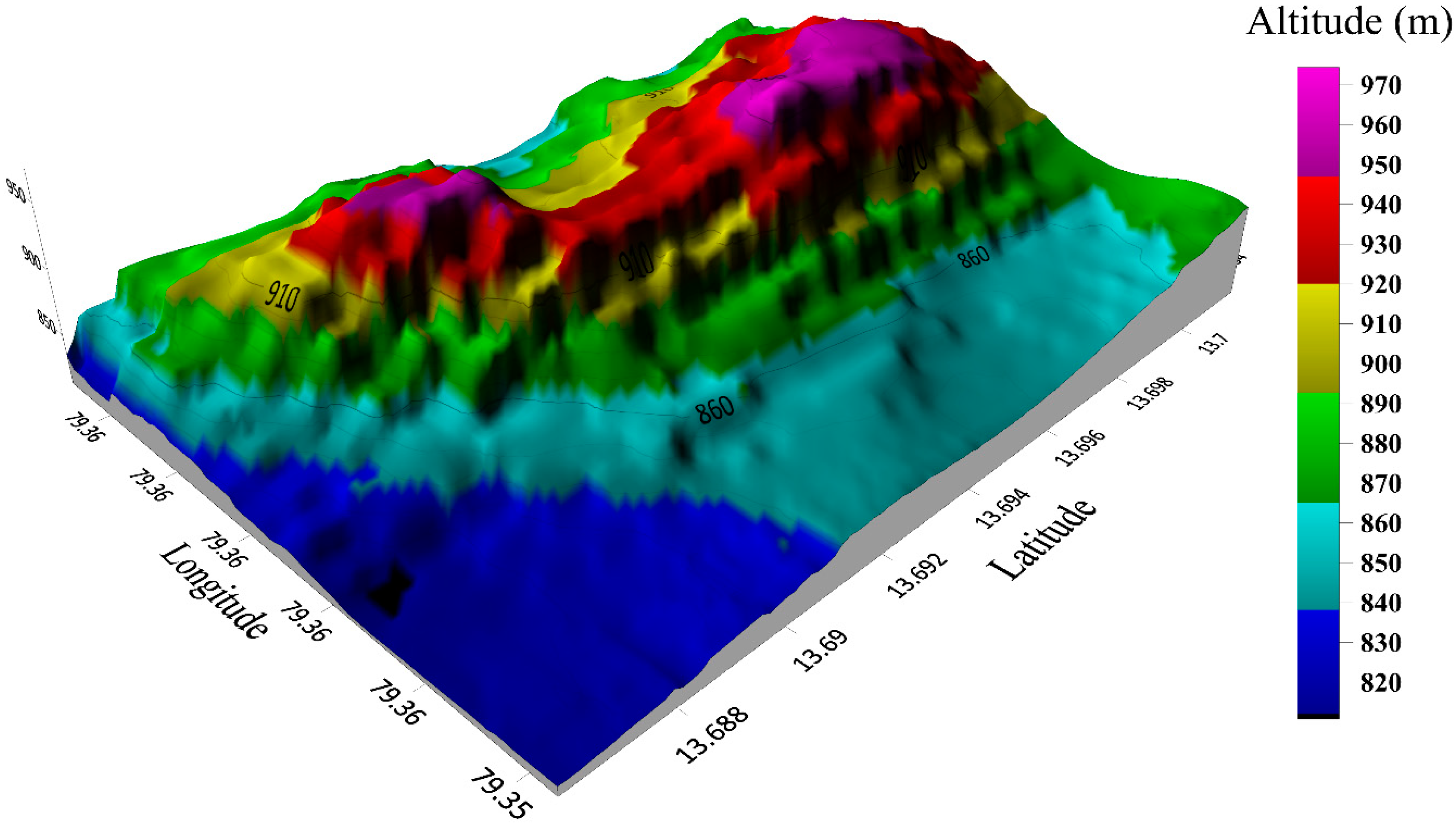
2.1. Location of Site and Collection of Wind Data

An Indian site, Tirumala (13°41′30.4″ N 79°21′34.4″ E), was selected for performing a statistical analysis of wind speed and direction. Hourly wind data was collected for a period of six years from 2012–2017. The site is probably a cool and humid place with better wind density. Tirumala is located at a distance of 28 km from Tirupati city of Andhra Pradesh. As per the 2011 census, the population of Tirupati is around 3.74 lakhs and due to its heavy population, this location was chosen for study. The wind speed and directions were measured using anemometers at two different hub heights of 10 m and 65 m. The measuring instruments were installed by the National Atmospheric Research Laboratory (NARL) located in Gadanki near Tirupati.
There were two important observation devices namely Doppler Sodar (MFAS64, SAMEER, Mumbai, Maharashtra, India), which is operated using a multi-frequency around (1600–2500 Hz) and the other was the UHF (ultra-high frequency) Wind Profiler (1280 MHz, PEC India, New Delhi, New Delhi, India). The measured hourly data was averaged monthly for the 10 m and 65 m height and shown in Figure 1. From Figure 1, it can be clearly observed that the maximum average wind speed available in the month of January was 4 m/s at 10 m and 5.2 m/s at 65 m. Similarly, the lowest average wind speed was present in the month of August and was 2.5 m/s at 10 m and 3 m/s at 65 m. The wind pattern slowly reduced from January and again reached to a maximum in the month of December.
The average wind speed ( v m ) and standard deviation ( σ ) were calculated using the following expressions:
v m = 1 n i = 1 n v i
σ = 1 n 1 i = 1 n ( v i v m ) 2
where, v i is the wind speed at ith hour and n is the number of hours. From this average value ( v m ), σ (standard deviation) can be calculated from Equation (2). For higher wind speed, the average value must be high and standard deviation should be low. As the standard deviation was low it shows that the dataset was more uniform.
The total number of data samples collected was 52,609 and from these 310 missing data were present and the remaining data were taken into consideration for the analysis. The surface plot for the selected site is shown in Figure 2 and these were obtained using ArcGIS software. From Figure 2 it can be stated that, the highest altitude was nearly 960 m from the sea level and the violet color shows an altitude of 960 m.

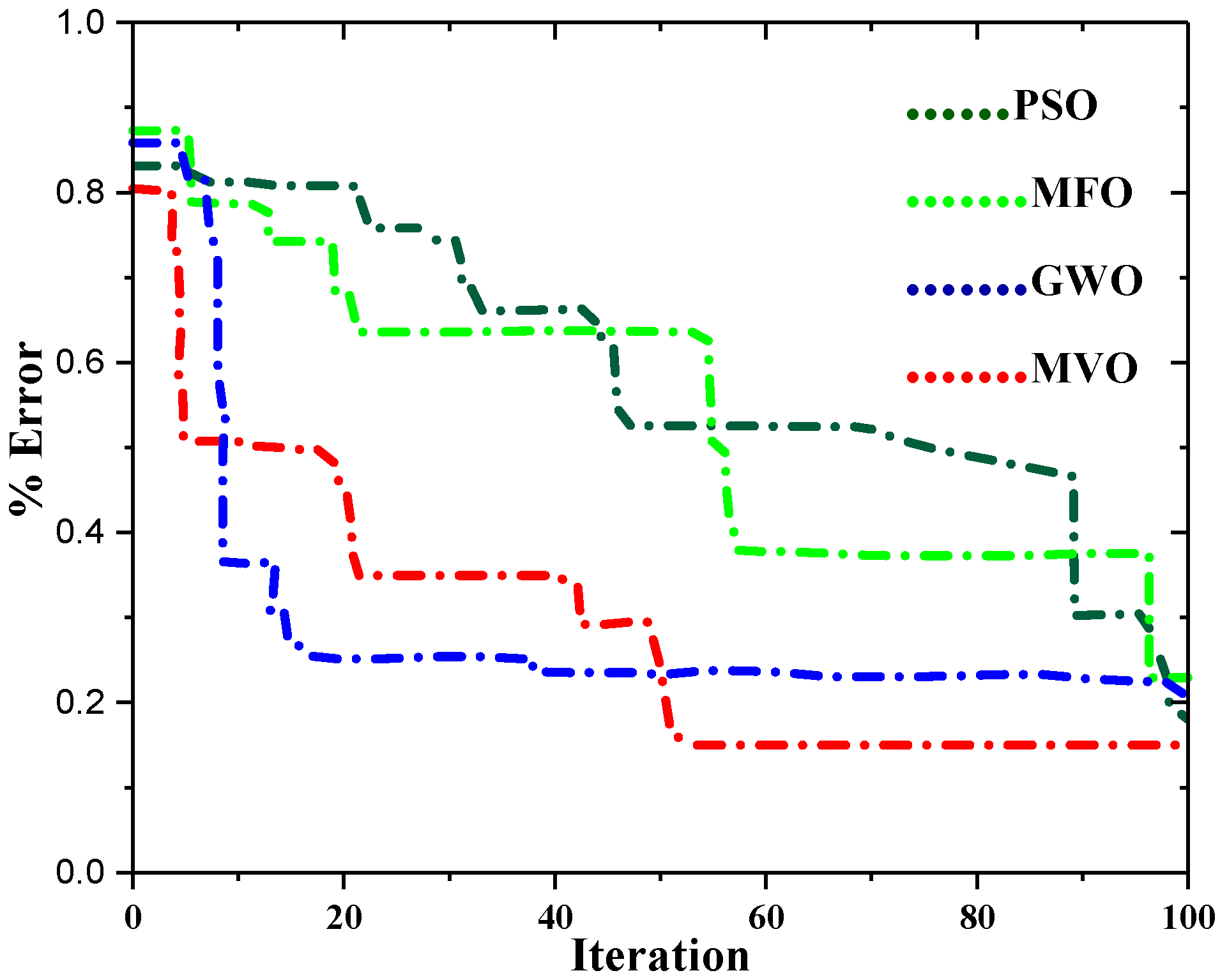
2.2. Multiverse Optimization Method for Parameter Estimation

The solution to any optimization problem involves artificial intelligence, which is used in various applications. This optimization includes probabilistic models of a natural occurring phenomenon to determine the optimal solution for a function. Though it gives a solution it does not guarantee the best one but it will converge quickly to the best.
Multiverse optimization (MVO) is one of the evolutionary techniques developed by Mirjalli, inspired by the concept of cosmology. The theory behind this is the white hole, wormhole and black hole and these are mathematically modelled in constructing the MVO. In this algorithm, the population is divided into two phases, i.e., exploration and exploitation. The white and black hole concepts are used to explore the search spaces. The wormholes will guide the MVO in exploiting the search space.
Here each solution resembles the universe, now each solution is assigned with some inflation rate and correlating with fitness function. The following rules are used in MVO:
When inflation rate is high, then probability of white hole is high;
When inflation rate is high, then black hole probability is low;
When the universe is having higher inflation rate, then it sends the object through white holes;
The objects will randomly move to the best universe through wormholes irrespective of inflation rate;
When inflation rate is low, then it receives the object from black holes.
For exchanging the objects in the universe, a roulette wheel mechanism was used. For every iteration the universe was sorted and the inflation rates were calculated to select the white hole among them. Let us consider:
U = [ x 1 1 x 1 2 . x 1 d x 2 1 x 2 2 . x 2 d . . . . . . . . x n 1 x n 2 . x n d ]
where d represents the number of variables and n is the number of universe (solutions);
x i j = { x k j r 1 < N I ( U i ) x i j r 1 N I ( U i )
where x i j is jth parameter of ith universe and Ui gives the ith universe, NI(Ui) is the normalized inflation of the ith universe, r1 is a random number between 0 and 1. x k j is the jth parameter of kth universe from roulette selection.
To avail the changes of each universe and to improve the inflation rate of wormholes, assuming that wormholes are present in between the universe and best universe. This can be shown below:
x i j = { { X j + T D R × ( ( u b j l b j ) × r 4 + l b j )   r 3 < 0.5 X j T D R × ( ( u b j l b j ) × r 4 + l b j )   r 3 0.5 x i j                  r 2 W E P r 2 < W E P
where x j represents the jth parameter and travelling distance rate (TDR), wormhole existence probability (WEP) are coefficients. The lower and upper bounds are shown as lbj and ubj for the jth variable. And rx are random numbers between [0,1].
The two main coefficients, WEP and TDR are used to define the existence in the universe and the travelling speed. This distance rate is a factor by which the object can be moved around the best universe. The expression for WEP is shown below:
W E P = min + l × ( max min L )
where the min value is taken as 0.2 and the max value to be 1, l indicates the iteration number and L is the maximum iteration number. Now, for TDR a similar mathematical equation is given below:
T D R = 1 l 1 / p L 1 / p
where p is taken as 6, defined for exploitation, the higher this value the faster the search. For improving the fitting curve, the variation between the Weibull distribution and actual wind speed distribution should be minimized. The objective function to be considered for minimization is given by:
ε ( v i ) = 1 2 i = 0 n ( f r e a l ( v i ) f w e i b u l l ( v i ) ) 2
where f r e a l ( v i ) gives the frequency of the wind speed class and f w e i b u l l ( v i ) gives the Weibull probability density function. The total number of wind speed classes is given by n.
In this present work multiverse optimization was implemented by taking 50 number of universes. In order to avoid premature convergence at initial stage the travelling speed and existence probability would vary. The lower and upper bound values were taken to be 0.4 and 0.9. The main reason to choose MVO was because it is a new meta-heuristic optimization technique inspired by the concept of cosmology and has not yet been tested for determining the Weibull parameters for wind energy applications.

3. Distribution Characteristics for Wind Data

The dynamic nature of wind can be studied with the application of the probability density function. The probability density function f(v) gives an idea about the occurrence of wind velocity and the cumulative distribution F(v) tells whether the wind velocity is less than or equal to that wind velocity. There are several methods that can be applied to analyze the wind data for estimating the wind potential [13,14] for a particular region. It was found from the literature that Weibull and Rayleigh [15] are the most preferred methods for determining the wind energy potential. In order to implement the Weibull and Rayleigh distribution, we need to estimate the shape and scale parameter. Many researchers have done studies for evaluating the wind potential through different probability density function. The results showed that the Weibull and Rayleigh distribution have presented the wind distribution in a better manner [16,17,18,19,20,21,22,23,24].

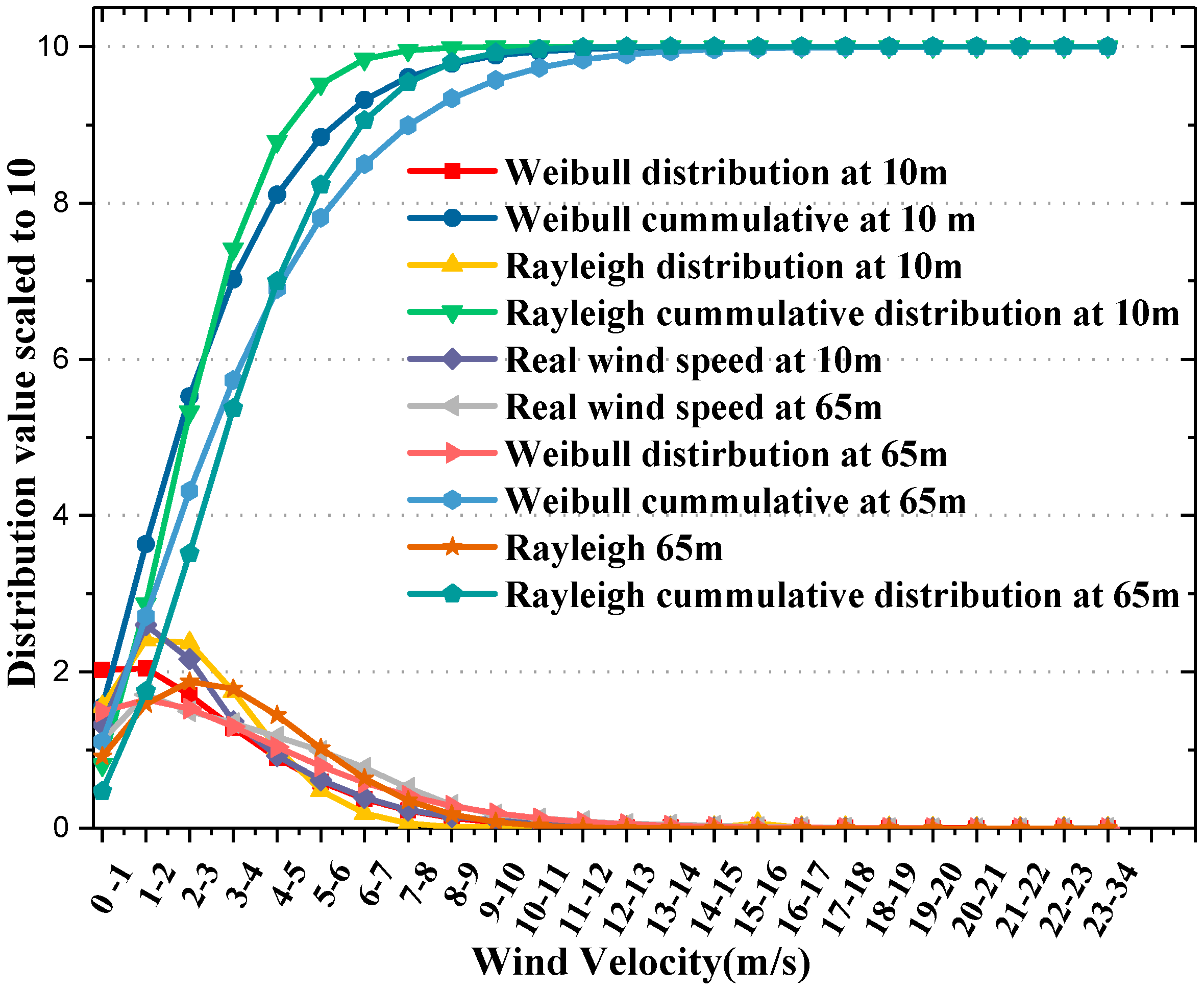
3.1. Weibull Distribution

This distribution has been used for many years for fitting source data, i.e., actual wind data. The wind data characteristics in any region can be analyzed by using the probability distribution function [25,26].
Another approach is to follow the Rayleigh distribution, which has also been used as one of the statistical tools to analyze wind data. To perform both Weibull and Rayleigh we required shape and scale parameters (k and c) [27]. The shape parameter value decides the type of distribution whether it should be Weibull or Rayleigh. When the shape parameter is less than 2 then it takes a Weibull distribution. When it is exactly 2 it is known as the Rayleigh distribution, if it exceeds 3 it takes the Gaussian distribution [28].
The Weibull distribution function or Weibull probability density function is calculated as [29]:
f ( v ) = ( k c ) ( v c ) k 1 e ( v c ) k
where, f ( v ) is the probability of wind speed, v is the wind velocity, k and c are the shape and scale parameters. k has no dimensional units whereas the c parameter has the dimensional unit as (m/s), similar to wind speed.
On integrating the Weibull probability distribution, we get the Weibull cumulative distribution function [30] and it is expressed as:
F ( v ) = 0 α f ( v ) d v = 1 e ( v c ) k
where α represents the highest wind speed under consideration and it changes according to the site.
The expected value of the wind speed otherwise known as the average wind velocity is obtained from the Weibull distribution parameters of k and c and is given by:
v m = c Γ ( 1 + 1 k )
where “Γ” is known as the gamma function and it is defined as:
Γ ( t ) = 0 x t 1 e x d x
Now the standard deviation for the Weibull distribution is given as:
σ = c Γ ( 1 + 2 k ) Γ 2 ( 1 + 1 k )
After calculating the values of σ and v m , the shape and scale parameters can be evaluated as follows:
( σ v m ) 2 = Γ ( 1 + 2 k ) Γ 2 ( 1 + 1 k ) 1
From expression (14) k can be found and once k is calculated, c is determined from the following:
c = v m Γ ( 1 + 1 k )
Now the Weibull probability density function is found using Equation (9).

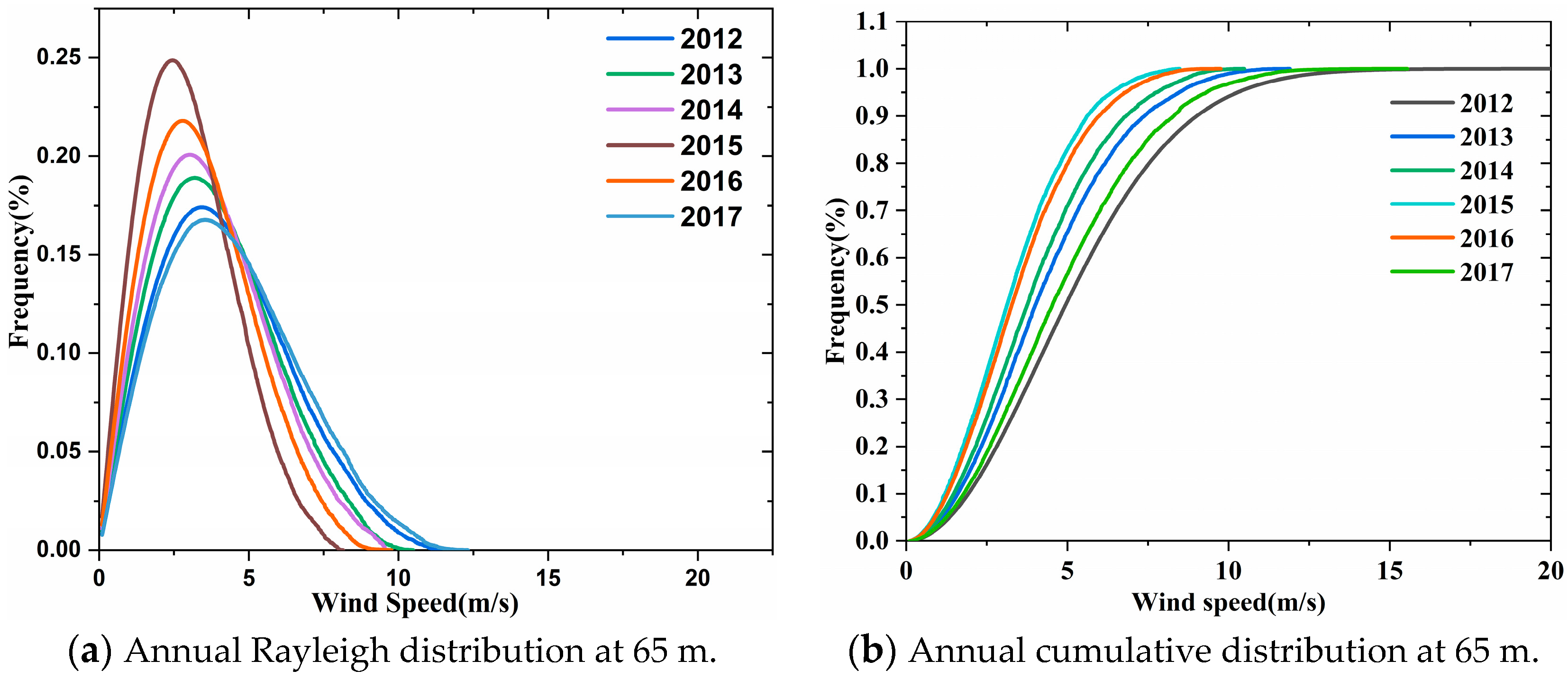
3.2. Rayleigh Distribution

It has already been mentioned that when shape factor “k” is 2 then such a distribution is known as the Rayleigh distribution [30]. Now after rearranging Equation (9), the Rayleigh probability density function is given by:
f ( v ) = ( v a 2 ) e v 2 2 s 2
where α is the scale parameter and its units are m/s and its value is given by:
α = 2 π v m
The Rayleigh cumulative distribution F(v) is calculated from the expression:
F ( v ) = 1 e ( v 2 2 α 2 )
In order to calculate the most probable wind speed ( V M P ) and the most energy ( V M a x E ) from the wind speed, it can be estimated from the equations as shown below:
V M P = c ( ( k 1 ) k ) k 1
V M a x E = c ( k + 2 k ) 1 k
There are many methods to determine the shape and scale parameters and few methods are the maximum likelihood, method of moments, least squares, graphical method, etc. All the software and tools used for statistical analysis are provided in Appendix A.

4. Results and Discussion

The study was carried out for the data collected from the region of Tirumala for about six years from 2012–2017. The data consisted of wind speed and wind direction collected from different hub heights of 10 m and 65 m. The monthly mean wind speed at 10 m and 65 m is shown in Figure 1. The shape and scale parameters for all the months have been calculated by using MVO. Table 1 presents the comparison of different numerical methods for estimating the Weibull parameters. For verification of the results, the MVO algorithm was compared with the moment method [14], empirical method [14], maximum likelihood [20], equivalent energy method [14] and energy pattern factor method [20]. Some of the meta-heuristic algorithms like PSO [20], MFO and GWO were also performed and are shown in Table 1.
The k and c parameters for the Weibull distribution were found using the moment method as expressed in Equations (21) and (22):
v ¯ = c Γ ( 1 + 1 k )
σ = c [ Γ ( 1 + 2 k ) Γ 2 ( 1 + 2 k ) ] 1 2
A special case of the moment method is the empirical method and it is determined using Equations (23) and (24) [31]:
k = ( σ v ¯ ) 1.086
v ¯ = c Γ ( 1 + 1 k )
The maximum likelihood needs extensive numerical iterations to find the k and c values and it is shown below in Equations (25) and (26) [31]:
k = [ i = 1 n v i k ln ( v i ) i = 1 n v i k i = 1 n ln ( v i ) n ] 1
c = ( 1 n i = 1 n v i k ) 1 k
The equivalent energy method [20] aims to determine the Weibull parameters by adjusting the wind data. The name is derived from the equivalence among the Weibull energy density curve and observed data energy density. From the below Equations (27) and (28), k and c values were estimated.
i = 1 n [ W v i e { ( v i 1 ) [ Γ ( 1 + 3 k ) ] 1 3 v 3 ¯ 1 3 } k + e { ( v i ) [ Γ ( 1 + 3 k ) ] 1 3 v 3 ¯ 1 3 } k ] 2 = i = 1 n ε v i 2
c = ( v ¯ ) 3 Γ ( 1 + 3 k )
The energy pattern factor method [24] is related with the average wind speed and is defined by Equations (29)–(31):
E p f = v 3 ( v ¯ ) 3
k = 1 + 3.69 ( E p f ) 2
v ¯ = c Γ ( 1 + 1 k )
The efficiency of meta-heuristic and other methods are determined using the correlation (r) and root mean square error (RMSE) equations as shown below:
r = i = 1 n ( X i X m e d ) . ( Y i Y m e d ) i = 1 n ( X i X m e d ) 2 . ( Y i Y m e d ) 2
R M S E = i = 1 n ( X i Y i ) 2 n
As shown in Table 1, MVO was compared with other numerical methods and a meta-heuristic technique for estimating the Weibull parameter and its r and RMSE were obtained. Among these methods the energy pattern method had the least k value of 1.5142 and its c value as 5.305. Other numerical methods generated different k values that does not fit the real wind pattern and the error was also more. When the RMSE value is low, then we can say that the real wind pattern fits the Weibull density function respective to the k and c values. In Table 1, after performing a statistical analysis it was found that MVO had the least error of about 0.0052 and it was less than 1%. The correlation value r was reaching to 100%, i.e., 0.995 for the study case. These values obtained from the proposed method were better than other numerical methods and meta-heuristic techniques. On comparing the GWO, PSO, MFO and MVO it was evident that MVO was performing better than other methods. The convergence curve was provided for the proposed method in comparison with the other method, it showed that MVO converged with less % error and in the minimum number of iterations as shown in Figure 3.
Table 2 shows the monthly k and c parameter, mean wind speed, standard deviation and the variance for both 10 m and 65 m height wind speed data. After calculating the k and c parameter for respective months, the most probable wind speed was calculated using Equation (19) and the maximum energy carried by the wind was obtained from Equation (20). These values were analyzed and presented in Table 2. From Table 2 it could be stated that the maximum average wind speed was about 5.12 m/s observed in the month of December at 10 m and in the same month about 6.621 m/s at the 65 m height, respectively.
For the complete dataset, the shape parameter varies from 1.27 at 65 m of hub height to 1.68 at 10 m of hub height. The shape and scale parameters for the entire dataset were found to be 1.47 and 4.806 m/s for 65 m height. For 10 m of hub height the average shape and scale values were 1.58 and 3.75 m/s. The most probable wind speed was calculated and found to be 4.02 m/s at 65 m height and 2.45 m/s at 10 m height. The maximum energy obtained from wind was 15.16 m/s and the lowest was 4.9 m/s. The minimum mean wind speed was present in the month of August with 2.43 m/s and the maximum was present in the month of December with 5.12 m/s at 10 m hub height. Similarly, at 65 m hub height the maximum and minimum mean wind speeds were 6.62 m/s and 3.17 m/s. The standard deviation values were found to have a minimum of 1.48 m/s and maximum of 4.65 for 10 m and 65 m hub heights.
Figure 4a,b shows the mean wind speed from 2012–2017 for all the months at 10 m and 65 m hub heights. From the graph it could be observed that the mean wind speed was maximum for February in the year 2016 and minimum mean wind speed for the month of September in the year 2017 at 10 m. Let us look into the mean wind speed at 65 m, the maximum means wind speed was observed to be 6.8 m/s in the month of February and minimum mean wind speed of 2.8 m/s for September in 2014.
The average wind speed lied in between 4 m/s and 6.8 m/s so we could conclude that there was sufficient wind potential in the region for installing small capacity wind turbines for extracting power from WECS. It could also be observed that the wind pattern varied as time progressed. This also reflected the effect of climatic conditions on the wind potential.
The Weibull probability density function was used to find the frequency of wind speed at different levels. After calculating the shape and scale parameters from the MVO method, the Weibull distribution and cumulative Weibull distributions were drawn. The graphs were obtained for all the years from 2012 to 2017 and were analyzed. From this distribution, it was easy to find the wind speed magnitude, which was more prevalent in this region. The frequency of occurrence of wind was slowly improving from 2012 to 2017 that could be clearly seen from the frequency of wind speed. From Figure 5a, the most prevalent wind speed was 4 m/s that occurred monthly with some percentage variation. This trend continued until 12 m/s to 15 m/s of wind speed. Later the frequency fell to zero, it meant that there was less chances of occurrence of wind speed beyond 16 m/s. Though it may exist but it did not influence the overall system performance. The Weibull cumulative distribution is shown in Figure 5b, which is the sum of individual Weibull distributions to reach 100%. The common point where all the graphs were meeting was at 16 m/s. In Figure 5b, between 8 m/s to 16 m/s all the wind was available and later it reached 100%, which meant that all the wind was available less than 16 m/s and after this there was less frequency of occurrence.
Rayleigh frequency distribution and Rayleigh cumulative frequency distributions are shown in Figure 6a,b. From this study, it revealed that the maximum probability for the wind fell in the range of 3 m/s to 6 m/s. The Rayleigh cumulative distribution also showed that 50% of the wind speed was between 3 m/s to 6 m/s. The frequency distribution was low for the wind speeds above 12 m/s. Therefore, we could say that the wind velocity above 12 m/s had less probability in this region. From Figure 6a,b the yearly frequency distribution was varying from 2012 to 2017 and the trend changed accordingly with the geographical parameters.
Now the actual wind speed at 10 m and 65 m hub heights was compared with the Weibull and Rayleigh distribution as shown in Figure 7. It could be seen that most of the wind speed occurred at less than 10 m/s. The Weibull cumulative distribution revealed that the maximum wind speed would fall in the range of 2 m/s to 12 m/s. Now, comparing these two distributions with real time wind data, it nearly coincided and hence concluded that the Weibull parameters fitted the actual wind pattern well. In Figure 7, the brown color bars indicate that the cumulative distribution values had reached maximum and it settled to 100%.
Table 3 shows the distribution of wind speed in terms of the Weibull and Rayleigh distribution. In Table 3 the Weibull and Rayleigh frequency distributions were scaled to the maximum value, and the cumulative distributions were scaled to 10 for better understanding. From this analysis, we can say that wind speed less than 9 m/s was more prevailing at the 10 m height and 3 m/s to 11 m/s at the 65 m height. There was an increase of wind speed distribution once the height increased so the more turbine height, the larger the power generation. Here it could also be concluded that Weibull and Rayleigh are a much similar distribution with a small change in the shape parameter value. Both the distributions were reaching the value of 10 approximately when it crossed 17 m/s of wind velocity. The real values and Weibull distribution value were better fitted and close to each other as we can see from Table 3. Once if we look into the real wind speed values at 10 m of hub height, all the values fell under the range of 12 m/s only, which is similar to the Weibull distribution. The same could be seen for 65 m, here the wind data ranged under 16 m/s due to the increase in hub height. Therefore, the Weibull parameter obtained from MVO was better suitable in understanding the wind pattern and wind potential at any location if we have good wind data.
The wind power density at 10 m and 65 m are shown in Figure 8a,b. From Figure 8a it could be inferred that the wind power density slowly increased from 4 m/s to 8 m/s, achieving maximum value, and later decreased to the reference level from 18 m/s. Compared to 10 m height, wind power density was having a much higher magnitude at 65 m. For 10 m, the power density tended to reach zero from 18 m/s but at 65 m the power density had a finite value until 24 m/s, so the wind power density could be improved by increasing the height of wind turbine hub from ground level. It could also be stated that due to an increase in the clearance area by removing the obstacles and landslide the wind circulation tended to improve yearly. The wind power density is improving from 2012 to 2017 for both 10 m and 65 m due to improvement in the clearance.
In order to quantify the Weibull and Rayleigh distributions with respect to actual data, few statistical analyses were performed.
The correlation coefficient ( R 2 ) value showed that the data is close enough to fit the regression line. The correlation parameter can be written as:
R 2 = i = 1 n ( y i z i ) 2 i = 1 n ( x i y i ) 2 i = 1 n ( y i z i ) 2
where yi is the real time observed wind data in the ith bin and xi gives the wind value from the Weibull distribution, zi is the mean value of yi and xi and n is the number of bins.
The chi-squared test ( χ 2 ) [4] was used to determine if there existed any difference between the expected and observed frequencies. In this statistical hypothesis test, the distribution was a chi-squared distribution when the null-hypothesis was true. The chi-square expression is as shown below in Equation (35):
χ 2 = i = 1 n [ ( y i x i ) 2 x i ]
The probability distribution is said to be accurate when R 2 is large with least χ 2 .
The Kolmogorov test [4] is a nonparametric test to compare the sample with a reference probability density function. For a given cumulative distributive function F ( v ) , the Kolmogorov test can be expressed as:
KOL = Max | F ( v ) F n ( v ) |
In the Equation (36), F(v) is the Weibull distribution and Fn(v) as the experimental histogram. It will consider only positive values and maximize the function for obtaining the result. This can only be performed when we have the cumulative distribution of the sample.
Sum of squares is determined by squaring the difference of mean value from individual observations and summing all those squared values. It gives information regarding the total variance of the observation. The sum of squares (SS) is expressed as in Equation (37) [32]:
SS = i = 1 n ( y i y ) 2
Another parameter, i.e., F-test [33] is used to compare the model for fitting the dataset and also to identify whether it best fits. The generalized F-test [33] expression can be written as given below in Equation (38):
F test = i = 1 K n i ( Y i ¯ Y ¯ ) 2 / ( K 1 ) i = 1 K j = 1 n i ( Y ij ¯ Y i ¯ ) 2 / ( N K )
where, Y i ¯ and Y ¯ are the ith group mean and overall mean and K represents the number of groups, whereas Y ij ¯ is jth observation from ith in k groups and N is the overall size.
In order to express the accuracy as a percentage of error we go for the mean absolute percentage error (MAPE) [33] and its mathematical equation is shown below:
MAPE = t = 1 n | A t F t A t | n 100
If, suppose we have to express the accuracy in same units then we prefer for mean absolute error (MAD) [29]:
MAD = t = 1 n | A t F t | n
For fitting the time series values and to measure the accuracy mean squared deviation (MSD) [32] is preferred and it is shown below:
MSD = t = 1 n | A t F t | n 2
In the above expressions, i.e., Equations (39)–(41), At and Ft are the actual and Weibull values with n as the total number of samples.
The t-stat [3] is a measure, which gives information about the ratio of estimated value to the standard error, and its expression is:
t stat = ( Actual   value forecasted   value ) ( n D 2 ( D ) 2 n 1
Now, the data taken for study was subjected to all these statistical analyses to determine various parameters and these are tabulated as shown in Table 4.
A model fits the data well when the difference of the observed value and the models predicted values are very small. In this case the R-squared measured the closeness of the data to the fitted regression. It is also gives the coefficient of determination so, the higher the R-squared value, the better the model fits the data. There is one limitation in R-squared, i.e., it does not indicate whether the model is adequate and sometimes a good model also might have a low R-squared value. Here in this study, the R-squared value lied between 0.90455 to 0.9898. Therefore, the model fitted the data well with R-squared values reaching nearer to 1, i.e., 100%.
Sum of squares (SS) deviations represents the sum of squared difference from the mean. In Table 4, SS was maximum in the month of August and minimum in the case of February. As the SS was low then we could say that, the values were closer to the mean, otherwise they were farther away from the mean so, the February month was having a low SS, which reflects that these values were closer to the mean. Another statistic applied was the F-test, when the calculated F value is high then we have to reject the null hypothesis. It was used to compare the models that were fitted to a dataset and to identify the model that best fitted the population from the data sample.
The MAPE is a measure of accuracy in predicting the values when we have a set of measured values. The percentage error measured how close the data points were present with respect to the predicted values. In Table 4, the percentage error was maximum for the month of December with 25.471% and least in the month of August with 6.4362%. As the percentage errors were less, it could be stated that the Weibull distribution nearly fitted the data. The mean absolute deviation (MAD) will measure the average distance from each value to the mean. It gives information on how the values are spread out in the sample space of the dataset. On observing the MAD values from Table 1, it is clear that all were less than 5 so, the Weibull distribution and the actual wind data were closely bound to each other.
Mean signed difference (MSD) is another statistic, which gives information on how well the estimate will fit the quantities that they were supposed to estimate. From Table 4, MSD values were 2.1627 for August followed by 2.671 for May and 3.371 April. Therefore, the estimated values were close to the measured values that had to be estimated and the maximum MSD was about 13.940 for December and 9.910 for January, which revealed that these values were unable to estimate better.
The chi-square, Kolmogorov and t-test were also performed to verify the Weibull distribution to fit the actual measured wind data. The chi-square values were maintained in between 0.018 to 0.073, which measures how much the actual observed data and expected values are present. KOL values ranged from 0.085 to 0.140 and were obtained by comparing the sample with the reference probability distribution. A T-test was used to know if there were any difference among the mean of the two groups of data.
The overall wind speed and wind directions are presented in Table 5 in the form of bin-sector and its distributions is shown in Figure 9. After analyzing Table 5 it is clear that the wind direction was most dominant between the sector 270–280° and 120–130°, having a frequency of 8.77% and 6.34%. It also suggested that the wind speed ranged from 2 m/s to 10 m/s in the above-mentioned sector directions. Whereas low wind speed flowed in the sector 170–180° from 0–4 m/s. Wind direction study showed that majority of the wind was flowing in the sector 260–280° that corresponded to SSW and NNW. The wind speed and direction graph for the months from January to June is shown in Figure 10.
The wind direction from 0–110° had a wind speed less than 14 m/s and beyond this there was no occurrence of any wind. From 110–200° the available wind speed was only below 12 m/s. There was large wind potential in the direction of 210° to 290° with a maximum wind speed reaching to 22 m/s, so if you install the wind turbines in this direction there is a possibility to increase the power generation. In future, short-term wind forecasting [34,35] can be performed by using an artificial neural network approach in combination with results obtained from the Weibull distribution and parameter estimation though nature inspired algorithms.

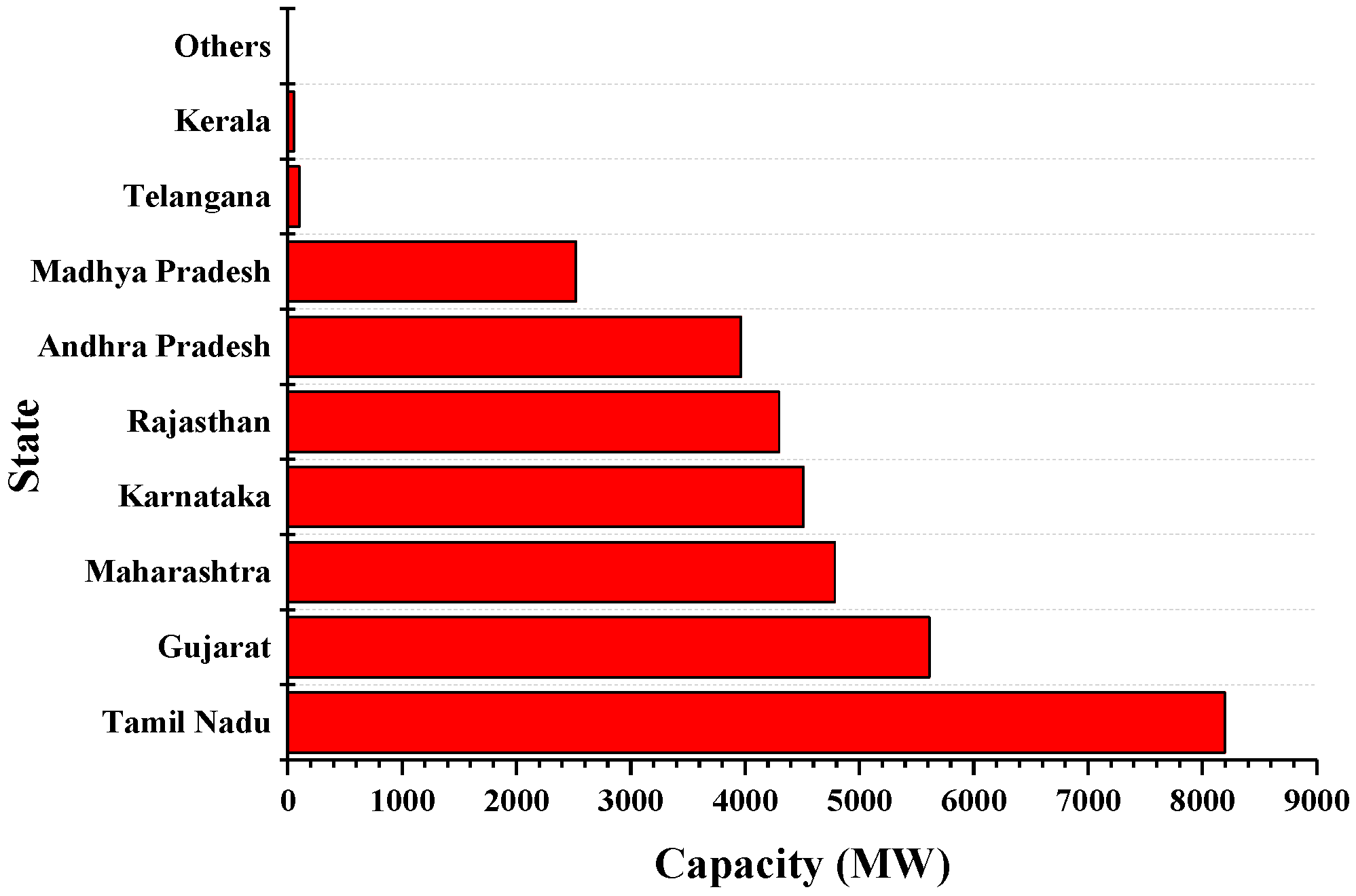
Comparison of Wind Farm Locations in India

In India, Tamilnadu is the top state in wind power generation and its contribution is around 29% of India’s total, wind generation for various states is shown in Figure 11. The importance of renewable energy and its need was realized in advance and established a new agency in 1985. The capacity of the Muppandal wind farm is 1500 MW and the total installed capacity in Tamilnadu is 7633 MW. Gujarath is focussing on enhancing renewable energy that has led to a sharp rise in wind power capacity. Based on government data the wind generation capacity has increased ten times in just six years. Next is the Mahastra with an installed capacity of 4655.25 MW. All major manufacturers of wind turbine including Vestas, Gamesa and Regen have their presence in Maharastra. In Kerala about 55 MW is installed and the first wind farm was installed in 1997 at Kanjikode in the Palakkad district. Recently offshore wind farms have started plans from 2010 and a 100 MW plant is located off the Gujarath coast that began in 2014. In order to identify potential sites GWEC developed R&D activities.

5. Conclusions

The study was done on wind data for a period of six years from 2012 to 2017 in the Tirumala region in India. Wind speed, wind direction, its frequency distribution, mean wind speed and k and c parameters for the Weibull distribution were calculated. The monthly wind direction was studied with a wind rose graph. The complete statistical analysis resulted in framing the following conclusions:
The shape and scale parameter (k and c) for the dataset was calculated and the observed data was fitted for Weibull distribution.
The highest mean wind speed was calculated as 6.621 m/s at 65 m and 5.12 m/s at 10 m for the month of December.
Annual mean wind velocity was calculated as 3.31 m/s and 4.36 m/s at 10 m and 65 m heights, respectively.
Wind speed with most energy (VmaxE) was calculated as 11.43 m/s and 15.16 m/s at 10 m and 65 m, respectively. The most probable wind speed was calculated as 2.45 m/s and 4.02 m/s at 10 m and 65 m, respectively.
From the cumulative frequency distribution it was found that the probability of wind speed for 4 m/s was predominant in the selected region.
The proposed method had few limitations such as computational complexity and it depended on the number of iterations, number of universes and universe sorting mechanism. The limitations also included the parameters to be estimated suffered from consistency when the measured wind data was not good. In order to achieve better results the measuring instrument must be properly calibrated before analyzing the data. The proposed MVO technique depended on the geographical location and also on the maximum and minimum wind speed limits. In future work, to forecast the wind speed, the MVO technique should be first implemented to find the Weibull parameters from the wind speed data and create hourly wind speed randomly. Now by applying randomly generated wind data to ANN for matching actual wind speed until the forecasted errors are minimized.

Author Contributions

All authors are involved developing the concept to make the article error free technical outcome for the set investigation work.

Funding

No funding received for this research work.

Conflicts of Interest

The authors declare no conflict of interest.

Appendix A

Table A1. Various tools and software’s used for simulation.
S. NoName of the Tool or SoftwarePurposeManufacturer Details
1MATLAB R2017bFor estimating shape and scale parametersR2017b, Math Works, Massachusetts, USA
2ArcGISContour plot10.6, Esri, Redlands, California, USA
3RStatistical analysis3.5, R Foundation of statistics, Vienna, Australia
4Surf plotSurface plot15.0, Golden software’s, Colorado, USA
5Origin2017ProGraphingSR1, Origin Lab, Massachusetts, USA
6ExcelFrequency distribution analysis, Bin-sectorV16.0, Microsoft Corporation, Redmond, USA

References

  1. Kumar, M.B.H.; Saravanan, B. Impact of global warming and other climatic condition for generation of wind energy and assessing the wind potential for future trends. In Proceedings of the Innovations in Power and Advanced Computing Technologies (i-PACT), Vellore, India, 21–22 April 2017; pp. 1–5. [Google Scholar]
  2. Huang, J.; Mc Elroy, M.B. A 32-year perspective on the origin of wind energy in warming climate. Renew. Energy 2015, 77, 482–492. [Google Scholar] [CrossRef]
  3. Shin, J.-Y.; Jeong, C.; Heo, J.-H. A novel statistical method to temporally downscale wind speed weibull distribution using scaling property. Energies 2018, 11, 633. [Google Scholar] [CrossRef]
  4. Gökçek, M.; Bayülken, A.; Bekdemir, S. Investigation of wind characteristics and wind energy potential in Kirklareli, Turkey. Renew. Energy 2007, 32, 1739–1752. [Google Scholar] [CrossRef]
  5. Kose, R.; Ozgur, M.A.; Erbas, O.; Tugcu, A. The analysis of wind data and wind energy potential in Kutahya, Turkey. Renew. Sustain. Energy Rev. 2004, 8, 277–288. [Google Scholar] [CrossRef]
  6. Keyhani, A.; Ghasemi-Varnamkhasti, M.; Khanali, M.; Abbaszadeh, R. An assessment of wind energy potential as a power generation source in the capital of Iran. Tehran. Energy 2010, 35, 188–201. [Google Scholar] [CrossRef]
  7. Dahmouni, A.W.; Ben Salah, M.; Askri, F.; Kerkeni, C.; Ben Nasrallah, S. Assessment of wind energy potential and optimal electricity generation in Borj-Cedria, Tunisia. Renew. Sustain. Energy Rev. 2011, 15, 815–820. [Google Scholar] [CrossRef]
  8. Kamau, J.N.; Kinyua, R.; Gathua, J.K. 6 years of wind data for Marsabit, Kenya average over 14 m/s at 100 m hub height; an analysis of the wind energy potential. Renew. Energy 2010, 35, 1298–1302. [Google Scholar] [CrossRef]
  9. Carrillo, C.; Cidrás, J.; Díaz-Dorado, E.; Obando-Montaño, A.F. An Approach to determine the weibull parameters for wind energy analysis: The case of Galicia (Spain). Energies 2014, 7, 2676–2700. [Google Scholar] [CrossRef]
  10. Kumaraswamy, B.G.; Keshavan, B.K.; Jangamshetti, S.H.; Member, S. A Statistical analysis of wind speed data in West Central Part of Karnataka based on weibull distribution function. In Proceedings of the IEEE Electrical Power & Energy Conference, 22–23 October 2009; pp. 1–5. [Google Scholar] [CrossRef]
  11. Murthy, K.S.R.; Rahi, O.P. Estimation of weibull parameters using graphical method for wind energy applications. In Proceedings of the Eighteenth National Power Systems Conference (NPSC), Guwahati, India, 18–20 December 2014. [Google Scholar]
  12. Zhang, L.; Li, Q.; Guo, Y.; Yang, Z.; Zhang, L. An investigation of wind direction and speed in a featured wind farm using joint probability distribution methods. Sustainability 2018, 10, 4338. [Google Scholar] [CrossRef]
  13. Shu, Z.R.; Li, Q.S.; Chan, P.W. Statistical analysis of wind characteristics and wind energy potential in Hong Kong. Energy Convers. Manag. 2015, 10, 644–657. [Google Scholar] [CrossRef]
  14. Kang, D.; Ko, K.; Huh, J. Comparative study of different methods for estimating weibull parameters: A case study on Jeju Island, South Korea. Energies 2018, 11, 6. [Google Scholar] [CrossRef]
  15. Wais, P. Two and three-parameter Weibull distribution in available wind power analysis. Renew. Energy 2017, 103, 15–29. [Google Scholar] [CrossRef]
  16. Akgül, F.G.; Şenoǧlu, B.; Arslan, T. An alternative distribution to Weibull for modeling the wind speed data: Inverse Weibull distribution. Energy Convers. Manag. 2016, 114, 234–240. [Google Scholar] [CrossRef]
  17. Mohammadi, K.; Alavi, O.; Mostafaeipour, A.; Goudarzi, N.; Jalilvand, M. Assessing different parameters estimation methods of Weibull distribution to compute wind power density. Energy Convers. Manag. 2016, 108, 22–35. [Google Scholar] [CrossRef]
  18. Boudia, S.M.; Benmansour, A.; Tabet Hellal, M.A. Wind resource assessment in Algeria. In Sustainable Cities and Society; Haghighat, F., Ed.; Elsevier: Amsterdam, The Netherlands, 2016; Volume 22, pp. 171–183. [Google Scholar]
  19. Carrasco, J.M.F.; Ortega, E.M.M.; Cordeiro, G.M. A generalized modified Weibull distribution for lifetime modeling. Comput. Stat. Data Anal. 2008, 53, 450–462. [Google Scholar] [CrossRef]
  20. Carneiro, T.C.; Melo, S.P.; Carvalho, P.C.; Braga, A.P.D.S. Particle swarm optimization method for estimation of Weibull parameters: A case study for the Brazilian northeast region. Renew. Energy 2016, 86, 751–759. [Google Scholar] [CrossRef]
  21. Costa Rocha, P.A.; de Sousa, R.C.; de Andrade, C.F.; da Silva, M.E.V. Comparison of seven numerical methods for determining Weibull parameters for wind energy generation in the northeast region of Brazil. Appl. Energy 2012, 89, 395–400. [Google Scholar] [CrossRef]
  22. Chang, T.P. Performance comparison of six numerical methods in estimating Weibull parameters for wind energy application. Appl. Energy 2011, 88, 272–282. [Google Scholar] [CrossRef]
  23. Saleh, H.; Abou El-Azm, A.A.; Abdel-Hady, S. Assessment of different methods used to estimate Weibull distribution parameters for wind speed in Zafarana wind farm, Suez Gulf, Egypt. Energy 2012, 44, 710–719. [Google Scholar] [CrossRef]
  24. Akdaǧ, S.A.; Dinler, A. A new method to estimate Weibull parameters for wind energy applications. Energy Convers. Manag. 2009, 50, 1761–1766. [Google Scholar] [CrossRef]
  25. Ouarda, T.B.M.J.; Charron, C.; Chebana, F. Review of criteria for the selection of probability distributions for wind speed data and introduction of the moment and L-moment ratio diagram methods, with a case study. Energy Convers. Manag. 2016, 124, 247–265. [Google Scholar] [CrossRef] [Green Version]
  26. Jaramillo, O.A.; Borja, M.A. Wind speed analysis in La Ventosa, Mexico: A bimodal probability distribution case. Renew. Energy 2004, 29, 1613–1630. [Google Scholar] [CrossRef]
  27. Wang, B.; Cot, L.D.; Adolphe, L.; Geoffroy, S. Estimation of wind energy of a building with canopy roof. Sustain. Cities Soc. 2017, 35, 402–416. [Google Scholar] [CrossRef]
  28. Pishgar-Komleh, S.H.; Keyhani, A.; Sefeedpari, P. Wind speed and power density analysis based on Weibull and Rayleigh distributions (a case study: Firouzkooh county of Iran). Renew. Sustain. Energy Rev. 2015, 42, 313–322. [Google Scholar] [CrossRef]
  29. Maatallah, T.; El Alimi, S.; Wajdi Dahmouni, A.; Nasrallah, S.B. Wind power assessment and evaluation of electricity generation in the Gulf of Tunis, Tunisia. Sustain. Cities Soc. 2013, 6, 1–10. [Google Scholar] [CrossRef]
  30. Spiropoulou, I.; Karamanis, D.; Kehayias, G. Offshore wind farms development in relation to environmental protected areas. Sustain. Cities Soc. 2015, 14, 305–312. [Google Scholar] [CrossRef]
  31. Wan, C.; Wang, J.; Yang, G.; Gu, H.; Zhang, X. Wind farm micro-siting by Gaussian particle swarm optimization with local search strategy. Renew. Energy 2012, 48, 276–286. [Google Scholar] [CrossRef]
  32. Ozay, C.; Celiktas, M.S. Statistical analysis of wind speed using two-parameter Weibull distribution in Alaçatı region. Energy Convers. Manag. 2016, 121, 49–54. [Google Scholar] [CrossRef]
  33. Safari, B.; Gasore, J. A statistical investigation of wind characteristics and wind energy potential based on the Weibull and Rayleigh models in Rwanda. Renew. Energy 2010, 35, 2874–2880. [Google Scholar] [CrossRef]
  34. Ali, S.; Lee, S.-M.; Jang, C.-M. Forecasting the long-term wind data via measure-correlate-predict (MCP) methods. Energies 2018, 11, 1541. [Google Scholar] [CrossRef]
  35. Chadee, X.T.; Seegobin, N.R.; Clarke, R.M. Optimizing the weather research and forecasting (WRF) model for mapping the near-surface wind resources over the Southernmost Caribbean Islands of Trinidad and Tobago. Energies 2017, 10, 931. [Google Scholar] [CrossRef]
Figure 1. Monthly average wind speed for 10 m and 65 m hub heights.
Energies 12 02158 g001
Figure 2. Surface plot of the selected site.
Energies 12 02158 g002
Figure 3. Convergence curve of multiverse optimization (MVO) in comparison with other meta-heuristic algorithms.
Energies 12 02158 g003
Figure 4. Monthly mean wind speed for 10 m and 65 m from 2012 to 2017.
Energies 12 02158 g004
Figure 5. Annual (a) Weibull and (b) cumulative distribution from 2012 to 2017 at 65 m hub height.
Energies 12 02158 g005
Figure 6. Annual (a) Rayleigh and (b) cumulative distribution from 2012 to 2017 at 65 m hub height.
Energies 12 02158 g006
Figure 7. Comparison of the Weibull and Rayleigh distribution with real wind data at 10 m and 65 m hub height.
Energies 12 02158 g007
Figure 8. Wind power density at (a) 10 m and (b) 65 m from 2012 to 2017.
Energies 12 02158 g008
Figure 9. Distribution of the wind speed based on the wind direction.
Energies 12 02158 g009
Figure 10. Wind speed-direction for the months from January to June in 2016 at 65 m.
Energies 12 02158 g010aEnergies 12 02158 g010b
Figure 11. Installed wind capacity by state as of 31st March 2018 in India.
Energies 12 02158 g011
Table 1. Comparison of different numerical methods with multiverse optimization.
Name of the MethodWeibull ParameterStatistical Test
kcrRMSE
Moment method1.59005.3260.9540.0149
Empirical method1.58675.3120.9530.0149
Maximum likelihood1.58105.3150.9670.0152
Equivalent energy method1.55115.3240.9780.0142
Energy pattern factor method1.51425.3050.9660.0151
PSO1.58265.3170.9630.0158
MFO1.54715.2640.9720.0175
GWO1.59845.3200.9840.0165
Multiverse optimization1.6265.3550.9950.0052
Table 2. Weibull parameters (k and c), monthly mean wind speed, Vmp, VmaxE, standard deviation and variance.
ParametersVmeanStd. DevVarianceckVmpVmaxE
Month10 m65 m10 m65 m10 m65 m10 m65 m10 m65 m10 m65 m10 m65 m
Jan4.085.333.23.8910.2215.124.435.781.471.412.073.147.9110.75
Feb3.524.832.463.176.05610.073.925.351.681.622.294.026.2598.76
Mar3.865.272.543.326.46311.034.285.861.651.542.453.976.90910.02
Apr2.933.791.892.33.5745.273.244.221.561.521.682.785.5147.302
May2.593.371.682.192.8114.773.564.121.571.501.882.625.9847.234
Jun2.723.431.942.443.7745.933.013.761.531.421.512.085.2036.941
Jul2.913.751.882.313.5215.353.253.711.701.371.941.835.137.13
Aug2.433.171.481.962.1873.843.013.531.601.641.642.714.9925.739
Sep2.843.832.022.594.0666.73.134.211.521.431.832.356.317.746
Oct2.913.822.012.624.0576.853.254.191.671.451.91.89 5.27.598
Nov3.865.102.453.146.0049.844.275.661.611.492.352.727.0589.968
Dec5.126.623.744.6514.0221.625.547.251.291.271.762.1911.4315.16
Aggregate3.314.362.32.885.568.873.754.811.581.471.942.696.498.7
Table 3. Weibull and Rayleigh frequency distribution compared with real data at 10 m and 65 m.
VjWeibull
10 m
Weibull
Cum 10 m
Rayleigh
10 m
Rayleigh
Cum 10 m
Real
10 m
Real
65 m
Weibull
65 m
Weibull
Cum 65 m
Rayleigh
65 m
Rayleigh
Cum 65 m
0 ≤ Vj < 12.0251.551.5530.811.3221.1251.4921.1080.91720.4698
1 ≤ Vj < 22.0463.6342.412.8672.6011.7101.6472.7121.58781.7509
2 ≤ Vj < 31.7075.5262.375.3242.1631.4941.5294.3151.87243.5150
3 ≤ Vj < 41.2847.0221.7497.4111.3681.3471.2985.7341.78255.3696
4 ≤ Vj < 50.8978.1061.0228.790.9221.1701.0376.9021.44496.9972
5 ≤ Vj < 60.5928.8430.4849.5220.6160.9890.7917.8141.02138.2313
6 ≤ Vj < 70.3729.3190.1899.8410.3930.7740.5818.4970.63749.0538
7 ≤ Vj < 80.2249.6120.0619.9550.2310.5160.4138.9910.35399.5403
8 ≤ Vj < 90.139.7850.0169.9890.1460.2990.2859.3370.17579.7971
9 ≤ Vj < 100.0739.8850.0159.9980.0980.1750.1929.5730.07829.9186
10 ≤ Vj < 110.049.940.0139.9990.0550.1260.1269.7310.03139.9704
11 ≤ Vj < 120.0219.9690.0119.9990.0380.0890.08129.8330.01139.9902
12 ≤ Vj < 130.0119.9850.019.9990.0210.0560.05119.8980.00369.9970
13 ≤ Vj < 140.019.9930.0099.9990.0130.0470.03169.9390.00109.9991
14 ≤ Vj < 150.0099.9960.0089.9990.0060.0320.01919.9640.00029.9998
15 ≤ Vj < 160.0089.9980.069.9990.0030.0150.01149.9796.88 × 10−59.9999
16 ≤ Vj < 170.0069.9990.005100.0020.0140.00679.9881.49 × 10−59.9999
17 ≤ Vj < 180.004100.004100.0010.0060.00389.9932.93 × 10−69.9999
18 ≤ Vj < 190.003100.003100.0010.0030.00229.9965.22 × 10−710
19 ≤ Vj < 200.002100.001100.0010.0010.00129.9978.41 × 10−810
20 ≤ Vj < 210.001100.001100.0010.0010.00069.9981.23 × 10−810
21 ≤ Vj < 220.001100.001100.0010.0000.00039.9991.62 × 10−910
22 ≤ Vj < 230.001100.001100.0010.0000.00029.9991.95 × 10−1010
23 ≤ Vj < 240.001100.001100.0010.0040.00019.9992.12 × 10−1110
Table 4. Monthly statistical parameters for evaluating the Weibull and Rayleigh distribution.
ParameterR2SSF-testMAPEMADMSDχ2Kolmogorovt-Stat
Jan0.98982120.5718.2412.1462.4069.9100.0180.1406.1205
Feb0.94262105.3415.0910.2051.8015.6980.0220.1345.357
Mar0.91533008.9440.2068.35581.71004.64460.0240.0958.637
Apr0.74573963.4246.91715.4361.5013.3710.0580.0898.8102
May0.91304557.4726.0410.7451.2962.6710.0420.0966.3874
Jun0.95924226.3930.95620.4791.5393.7640.0470.1287.0846
Jul0.904554191.5431.0017.13651.49983.45990.0510.1117.38159
Aug0.92825116.0921.97196.43621.11292.16270.0240.0866.016
Sep0.95434054.4428.39517.8691.4503.8560.0950.1266.8898
Oct0.92104261.2526.21611.6131.6024.0480.0640.1546.5784
Nov0.9792827.2163.90017.101.8365.3290.0730.08510.8828
Dec0.913932269.2996.23525.4713.09313.9400.0230.11213.3726
Table 5. Distribution of the wind direction based on wind speed frequency.
Wind DirectionWind Speed (m/s)
0–22–44–66–88–1010–1212–1414–1616–1818–2020–2222–24Total
0–100.42%0.36%0.36%0.31%0.08%0.01%0%0%0%0%0%0%1.55%
10–200.54%0.27%0.19%0.13%0.05%0.01%0%0%0%0%0%0%1.18%
20–300.51%0.2%0.12%0.05%0.02%0.01%0%0%0%0%0%0%0.9%
30–400.53%0.21%0.1%0.03%0.02%0.01%0%0%0%0%0%0%0.89%
40–500.43%0.22%0.12%0.06%0.02%0.01%0%0%0%0%0%0%0.86%
50–600.48%0.24%0.16%0.1%0.02%0.01%0%0%0%0%0%0%1.02%
60–700.54%0.29%0.19%0.11%0.07%0.02%0%0%0%0%0%0%1.22%
70–800.71%0.42%0.24%0.2%0.1%0.02%0%0%0%0%0%0%1.7%
80–900.52%0.51%0.34%0.33%0.07%0.02%0%0%0%0%0%0%1.78%
90–1001.6%1.45%0.62%0.25%0.06%0.01%0%0%0%0%0%0%3.99%
100–1101.05%1.63%1.05%0.32%0.05%0.02%0%0%0%0%0%0%4.12%
110–1200.96%1.82%1.78%0.93%0.22%0.04%0.01%0%0%0%0%0%5.76%
120–1301.08%1.94%1.69%1.38%0.24%0.02%0%0%0%0%0%0%6.34%
130–1401.08%1.24%0.62%0.37%0.04%0%0%0%0%0%0%0%3.35%
140–1500.88%0.7%0.33%0.07%0%0%0%0%0%0%0%0%1.98%
150–1600.77%0.42%0.17%0.02%0%0%0%0%0%0%0%0%1.39%
160–1700.6%0.31%0.13%0.03%0%0%0%0%0%0%0%0%1.07%
170–1800.35%0.28%0.12%0.02%0%0%0%0%0%0%0%0%0.78%
180–1901.28%0.43%0.18%0.06%0%0%0%0%0%0%0%0%1.95%
190–2000.52%0.36%0.25%0.06%0.01%0%0%0%0%0%0%0%1.21%
200–2100.44%0.31%0.22%0.18%0.05%0.02%0.01%0%0%0%0%0%1.22%
210–2200.49%0.43%0.27%0.21%0.12%0.06%0.04%0.01%0.02%0.01%0%0%1.63%
220–2300.57%0.42%0.39%0.23%0.18%0.11%0.04%0.05%0.02%0.01%0%0%2.03%
230–2400.5%0.59%0.58%0.34%0.23%0.12%0.07%0.03%0.02%0%0%0%2.47%
240–2500.62%0.73%0.89%0.7%0.35%0.33%0.23%0.1%0.05%0.01%0%0%4.01%
250–2600.66%0.98%1.14%1.12%0.74%0.4%0.21%0.12%0.05%0%0.01%0%5.44%
260–2700.53%1.03%1.6%1.33%0.72%0.38%0.21%0.07%0.02%0.01%0.01%0%5.92%
270–2801.63%1.92%2.36%1.72%0.68%0.26%0.12%0.06%0.02%0.01%0%0%8.77%
280–2900.99%1.44%1.44%0.78%0.3%0.15%0.06%0.04%0.01%0%0%0%5.2%
290–3000.99%1.17%0.76%0.35%0.1%0.05%0.01%0.01%0%0%0%0%3.44%
300–3100.92%1.08%0.46%0.16%0.04%0.02%0%0.01%0%0%0%0%2.68%
310–3200.95%0.92%0.33%0.09%0.02%0.01%0%0%0%0%0%0%2.32%
320–3300.89%0.96%0.38%0.08%0.03%0.01%0%0%0%0%0%0%2.34%
330–3400.82%1.08%0.56%0.15%0.04%0.01%0%0%0%0%0%0%2.66%
340–3500.87%1.17%0.72%0.25%0.07%0.01%0%0%0%0%0%0%3.1%
350–3601.41%0.93%0.8%0.46%0.08%0.04%0.01%0%0%0%0%0%3.72%
Total28.13%28.47%21.64%12.98%4.8%2.17%1.03%0.49%0.21%0.05%0.02%0.01%100%

