1. Introduction
Recently, energy production has been investigated widely due to the risk of energy crises and global climate change. The production of renewable energy performs an essential role in the economic growth of a country. Wind power is considered a necessary resource for electrical power production. The installed capacity of wind farms worldwide has increased 30 times to a total of 435 GW, with 17% cumulative growth in the last few years. In 2020, wind energy is expected to supply approximately 12% of the total worldwide requirement [
1,
2].
The uncertain features and lower controllability of wind power raises the problems of power stability and reservations to the power systems [
3]. Furthermore, wind speed may be easily affected by height and different types of obstacles. Therefore, intelligent and accurate power forecasting tools are required to improve the accuracy of stable power predictions and decrease operational costs. Many kinds of research have designed different types of algorithms to forecast wind power. Commonly, the wind power forecasting methods are divided into three main categories, i.e., numeric weather prediction (NWP), statistics-based and hybrid [
4,
5]. Mathematical models are designed to predict valid NWP, which is more valuable for longer horizons in terms of accuracy. However, it is hard to develop an exact mathematical model without the in-depth knowledge of physics and atmosphere. Such a model uses different methodological factors which are hard to measure.
Statistical methods are used to predict the correlation among various features of historical wind data with the help of explanatory variables. These require only wind data for forecasting, and thus, these tools are of particular interest for different types of engineering applications. The prediction accuracy of statistical methods decreases in long forecasting horizons.
The artificial neural network (ANN) [
6], convolution neural network (CNN) [
7], support vector regression (SVR) [
8] and back propagation neural network (BPNN) [
9] are the most-used statistical methods. The ANN is a framework which further contains different machine learning algorithms to process the complex type of data. Such kinds of algorithms learn from data samples and then accomplish specific actions according to inputs. The CNN is a particular type of artificial neural network which uses a perceptron to analyze data in supervised learning. The BPNN is used to calculate the weights based on gradients in the neural network, and generalizes the feedforward in a multilayer neural network. It uses a chain rule to compute the gradient in a loop manner for each layer.
Time series-based models also use wind farm historical data (mainly in minutes or hours) for wind speed and power forecasting. These are useful for ultra-term low wind signals because they can extract the hidden stochastic characteristics. The models include Box–Jenkins models [
10], Kalman filters [
9] and ANN [
11]. The Box–Jenkins model is a time series model that works on nonlinear estimation, so upcoming observations may not be expended to modify parameters directly. Complete assessment can require complex calculations. The Kalman filter, also known as a linear quadratic estimator, uses a finite linear estimated value for forecasting future values so needs less calculations as compared to Box–Jenkins. Thus, Box–Jenkins yields better accuracy but needs a large level of calculations as compared to Kalman filters. The Kalman filter is best for a smaller number of observations and predictions. The ANN has received attention for dealing with real-time behavioral data because such data may be extremely nonlinear. It uses neural network algorithms, such as a multilayer perceptron, but does not fully employ a systematic manner because of its formal specification [
12,
13]. The prediction competency of statistical methods declines in longer forecasting horizons. On the other hand, our proposed TensorFlow-based deep learning approach may be configured according to requirements. We may add dense layers, a number of neurons, an optimizer function and dropout layers to get better accuracy. We fine-tuned the designed approach with dropout layer parameters to resolve the overfitting problem on large scale wind data.
However, the existing state of the art methods still did not predict the required power forecast. It is essential to explore different characteristics of wind power for designing an accurate model. Wind speed follows the Gaussian distribution, and the bet distribution and loss function depends on the type of delivery [
14]. The hybrid method is a combination of two or more techniques. The hybrid approach using wavelet transform (WT) and fuzzy ARTMAP (FA) is proposed to forecast the deterministic wind power. The support vector machine (SVM) is used to classify wind power forecast error for the decomposed features acquired from WT and FA. The proposed idea is investigated using Cedar Creek wind farm data for probabilistic forecasting performance [
15]. The deep learning models significantly improve the wind power forecasting accuracy as compared to the existing machine learning algorithms. The multilayer perceptron (MLP) is used to optimize the weights, and a CNN is used to mine the spatial feature structure. The proposed research is used to predict the NWP [
16]. In hybrid methods, the auto-regressive integrated moving average (ARIMA) model is typically used for linear behavior and the SVM, while the ANN is used for nonlinear behavior [
17]. The ARIMA is used to forecast the future time series points based on the historical data. Depending on the area of the horizon, the hybrid methods have performed better than individual ANN or SVM. The SVM is a supervised learning model that is used to analyze data investigated for classification and regression evaluation. The hybrid methods gave better results in short-term forecasting but did not compete with other optimized algorithms [
18].
In the last few years, different hybrid wind power forecasting techniques have been proposed. Usually, the forecasting accuracy of hybrid approaches is as least as good as that of individual methods. Generally, hybrid methods are categorized into two classes [
19]. First, the hybrid approach calculates weighting coefficients of each technique and then, adds them to give a total weighted prediction. In [
20], the author proposed a hybrid method of grey rational analysis and distributed features of wind speed with cumulative weighting coefficients. It combined two algorithms, the least square support vector machine (LSSVM) with the radial basis function neural network (RBFNN). The results have shown that the combined approach achieved better forecasting accuracy than individual models for short-term data. In [
21], the author proposed the hybrid method of artificial intelligence-based algorithm and contrary constraint theory to forecast wind energy. The weighted features were extracted using chaos optimization and genetic algorithms. The hybrid approach improved forecasting accuracy by combining the meaningful features of individual techniques. Secondly, the pre-processing method was used to retrieve essential features from nonlinear wind speed data. It was used to convert highly correlated data into more linear and normalized factors. Recently, extensive use has been made of different large-scale decomposition techniques integrated with hybrid forecasting models. In [
22], four different hybrid models were proposed to obtain a significant increase in multi-step wind forecasting accuracy, combining decomposition techniques, i.e., wavelet decomposition, wavelet packet decomposition, empirical mode decomposition and false ensemble empirical mode decomposition.
The extreme learning machine (ELM) algorithm is used for wind forecasting prediction and classification. The ELM is employed in feedforward neural networks used for classification, regression, clustering and feature learning based on input weights with single or multi-layer architecture. In [
23], the combined approach of Beveridge–Nelson decomposition (BND), relevance vector machine (RVM) and Ant Lion Optimizer (ALO) is used. First, the author used the time series algorithm to decompose the nonlinear data to deterministic and meaningful features. The BND algorithm was used to extract the normalized stochastic components. Then, RVM is used to predict the wind forecasting accuracy from already decomposed components. The proposed methodology is applied to the hourly real-world wind power data collected from the Xinjiang region in China. In [
24], two combined methods, i.e., fast ensemble empirical mode decomposition (FEEMD) and MLP neural network are used to improve the prediction accuracy. The FEEMD algorithm is used to convert the historical data into different useful sub-layers, and MLP is applied to predict the specific layers accurately. The combined approach of BPNN and SVM is used to analyze the wind farm data statistically for forecasting of power and error probability distribution. The critical phase is to compute the corresponding uncertainty value for prediction. The combination of error estimation and error probability distribution is investigated using the historical data of seven wind turbines for NWP. The results show that the proposed methods provide improved results for short-term wind speed [
25]. Twenty-four hours of wind speed data are analyzed and forecasted with a state estimation-based neural network (SENN). The proposed method used weighted least square state estimation (WLSSE) for predicting the input and output hidden layers. The results have shown that prediction accuracy is better than using a BPNN [
26]. The combined approach of a back propagation (BP) algorithm with stacked auto-encoders (SAE) is proposed. The SAE based on a neural network is used to retrieve the hidden features from the different sequence and, then, the loss function is used to obtain the optimal connected weights. The BP algorithm is applied to fine-tune the values in the neural network. Particle swarm optimization is used to select the optimal number of neurons in the hidden layer and the learning rate. The results have shown that the proposed method yields better accuracy as compared to a SVM and neural network [
27].
Principal component analysis (PCA) is a statistical technique that can be used to decompose the raw historical wind speed data into reduced useful features. In [
28], PCA is also known as the empirical orthogonal function (EOF), which is used to retrieve the hidden patterns from the ocean-related and climatological data. Now, it is widely used in time series data analysis with nonlinear features. It is a potent tool to mine useful information and remove the noisy data in nonlinear dynamic systems [
18,
29,
30]. The FEEMD algorithm is used to transform the wind power time series into various sub chains. PCA is applied to extract the reduced features’ matrix preserving the actual information. Then, the reduced patterns are analyzed using the LSSVM and bat methods. Further, the author explained that PCA data inputs increased the overall accuracy by preserving the actual information [
31]. Deep learning can be used for predictions of useful layers in the extensive collection of big data. PCA is used to extract valuable samples from noisy data. Then, the long short-term memory (LSTM) neural network is applied to the principal components for numerical weather prediction. The results have shown that the hybrid approach of PCA with deep learning has better accuracy than a SVM and BP neural network [
32]. The LSTM algorithm from the TensorFlow database is used to predict the interaction of wind turbines. PCA is applied to get the reduced dimensions of the highly correlated time series data. Then, the LSTM is used to analyze the beneficial relationship among the selected features of the wind turbine data. The proposed methodology is compared with BPNN and ARIMA for forecast errors. It is shown that the hybrid model of PCA and LSTM increases prediction accuracy [
33]. The combination of PCA and independent component analysis (ICA) is used to reduce mutual interference among different parameters and retrieve the independent components. Further, these components are merged with the RBF network to predict the actual characteristics of wind farms and to improve accuracy [
34].
Large-scale wind power forecasting is the main focus of many researchers [
35]. The most useful approach is to forecast power production over different regions based on hourly, monthly and yearly historical data collected from wind turbines. In this paper, we have proposed a hybrid approach of optimized deep learning and PCA to forecast the wind power for large-scale historical data. First, PCA is used to expose the hidden patterns and to retain the most significant information [
18,
36]. PCA is applied to the historical wind data over the entire grids and eigenvalues and eigenvectors are calculated. This reduces the matrix size by focusing on the critical features and removing noisy data. TensorFlow is an online open source software library for numerical computation using dataflow graphs. The optimized deep learning algorithm using TensorFlow is applied to the reduced data features to predict the forecasting errors [
37]. It uses a neural network to predict the relationship between data features. The wind power depends on the cubic of the wind speed, as it follows the wind power curve.
The paper contributions are:
Reduced useful features are extracted from the massive-scale wind turbine data, i.e., hourly, monthly and yearly;
The deep learning algorithm is configured using the TensorFlow framework with Keras for prediction of wind forecast parameters;
The deep learning algorithm is optimized with fine-tuning parameters, i.e., dropout layer, dense layer, learning error rate, loss and activation function;
A comparison is made with state-of-the-art techniques.
Section 2 describes PCA in details,
Section 3 explains the deep learning model using the TensorFlow framework,
Section 4 presents the results and discussion, and
Section 5 concludes.
2. Principal Component Analysis
It is difficult to analyze high dimensional datasets and to make inferences for further experiments. PCA is a statistical technique that converts highly correlated variables into reduced uncorrelated variables while preserving the actual information of the data. It transforms the high dimensions of large datasets by calculating eigenvectors, also known as principal components (PCs). The resultant PCs map the high variance of these large datasets into eigenvalues. There are several PCs that may be computed by PCA in such a way, so that the first PC covers the highest variance, the second PC covers the second highest variance, and so on. This removes the noisy data and maps complex data into simple principal components, which simplifies further predictions analysis. The PCs preserve the actual information of the data. We select those PCs for prediction purposes which collectively cover more variance, making it easier to perform predictions with better accuracy. PCA is a statistical technique which extracts a set of defined and useful features from raw data by using orthogonal transformation [
38,
39]. Wind farm data is mostly collected in raw form and needs to be cleaned of noisy data. We used PCA to process complex wind datasets into simple PCs. Mathematically,
dimensional vectors with individual coefficients are shown in Equation (1).
where
denotes the unit vector and
k is the linear number. It transforms each data cell (
) in wind farm data to a linear form of principal components scores as shown in Equation (2).
where
defines the captured variances from each data cell. The components’ weights are computed as shown in Equation (3).
where
= 1, …,
and k = 1, …,
;
denotes the maximum possible variance with the
coefficient vector for each variance. The principal components’ scores are captured in such a way that the first principal component covers the highest variance from wind data. Further, each successive component extracts the next highest variance.
Mathematically, the first principal component (PC1) is defined as shown in Equation (4).
where
is the principal component and
denotes the data cell in the wind data. Similarly, the
principal component is calculated by subtracting the first
from
using Equation (5), where
represents the data matrix.
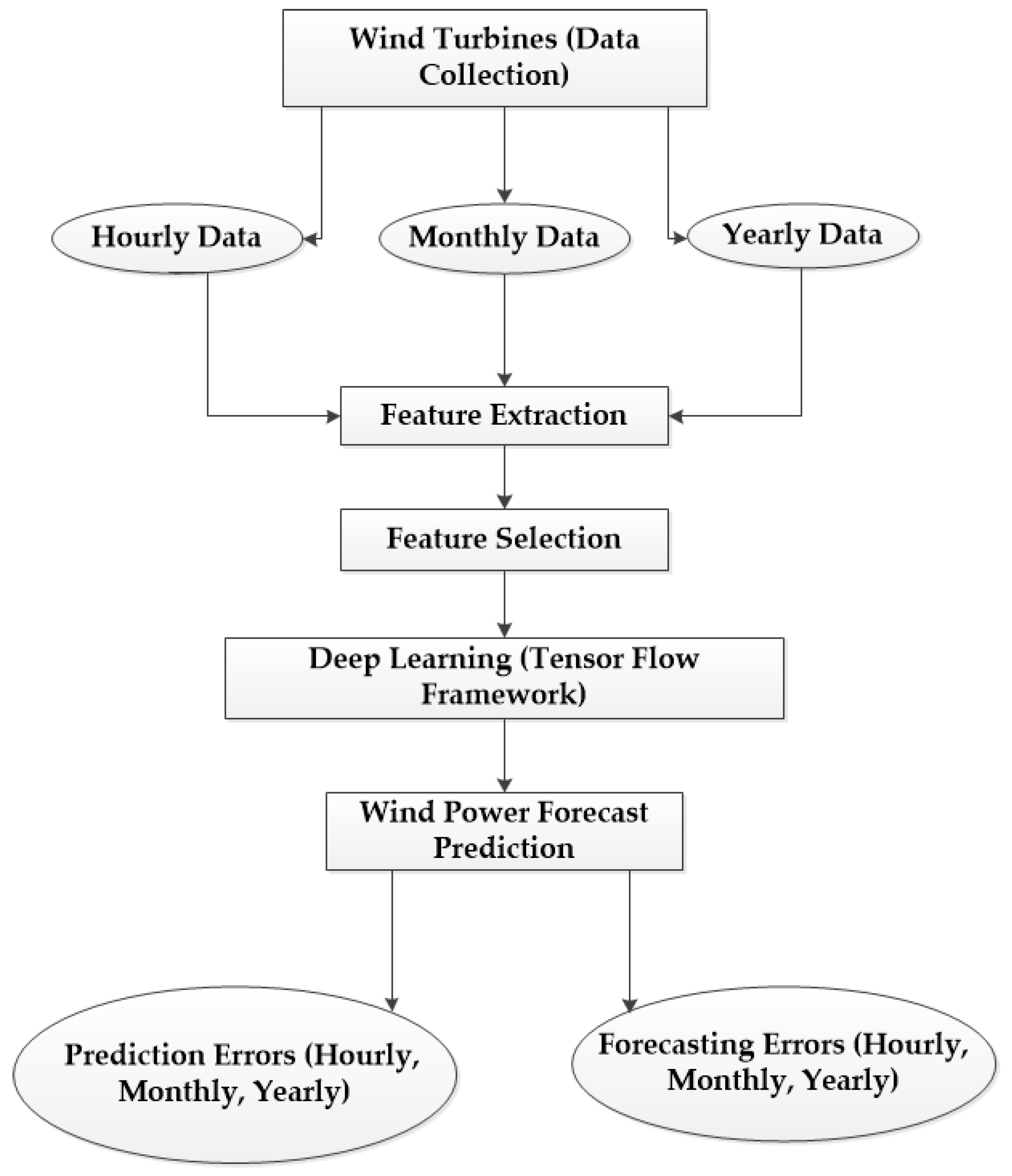
This retrieves values in the normalized form in a range of −1 to +1 [
40]. The complete flow of methodology steps as shown in
Figure 1.
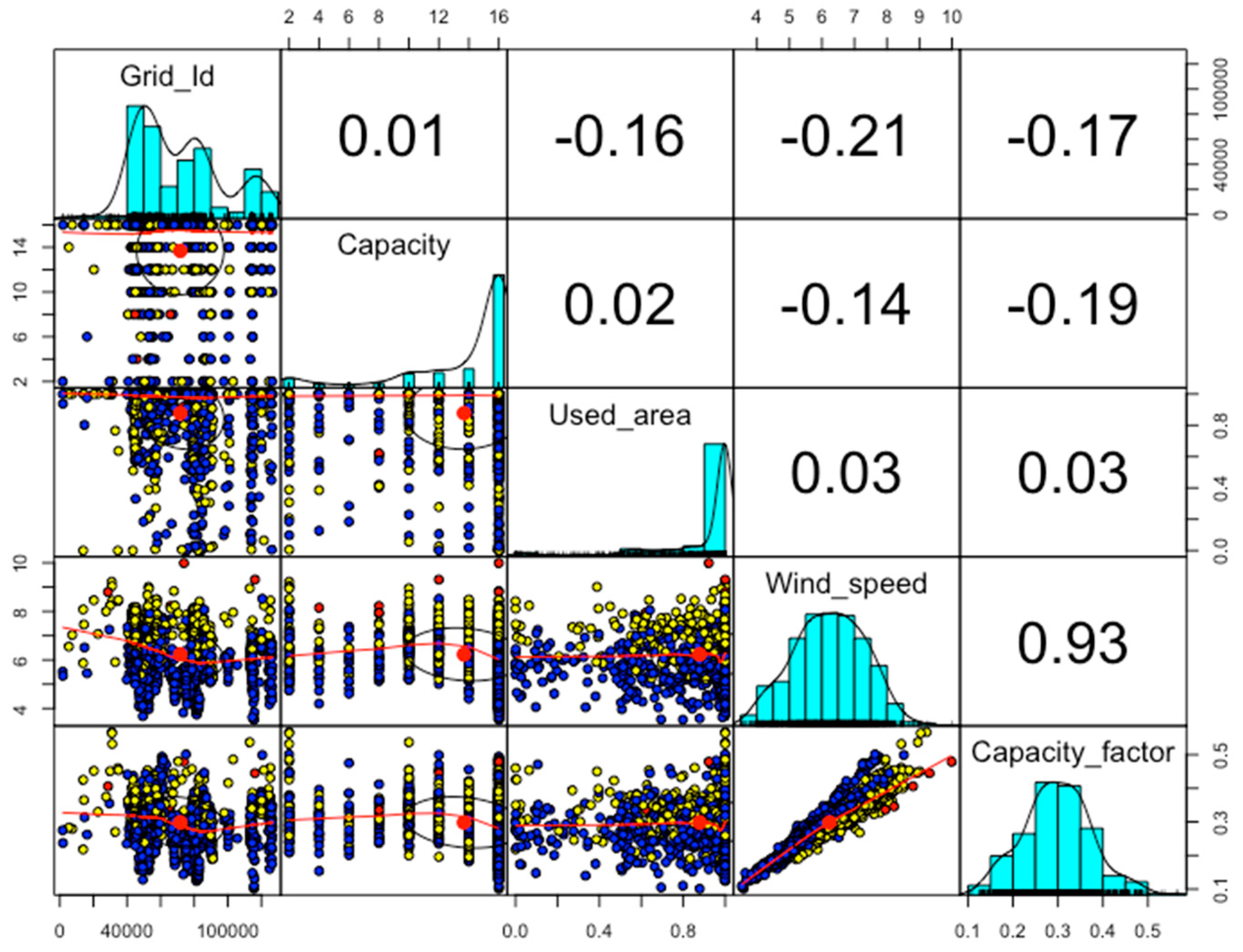
The principal components are then used as input data to deep learning based on the TensorFlow framework. PCA provides feature extraction and selection. The proposed research is examined with three different datasets collected within the NREL database in the US. These three datasets contain hourly, monthly and yearly real-time wind turbine data. First, the hourly wind dataset is collected from 20 m to 160 m distance on the ground and with a duration of 1 h, 4 h and 6 h, respectively. It contains the data of 126,000 wind farm sites with different meteorological parameters. Second, the monthly wind dataset is collected from the Hawaii region of the US with the mean of a 2 km grid in January. This data contains the cumulative average of 17 years of Modern-Era Retrospective analysis for Research and Applications (MERRA) time series data collection from different wind turbines. Third, the yearly dataset is collected from an offshore wind statistics geodatabase that captures different wind speed parameters for Hawaii. The real-time historical data is analyzed by the MERRA time series for 17 years and collected as a commutative average of the different meteorological parameters from approximately 2 km grids. The hourly wind data has highly uncorrelated data as shown in
Figure 2.
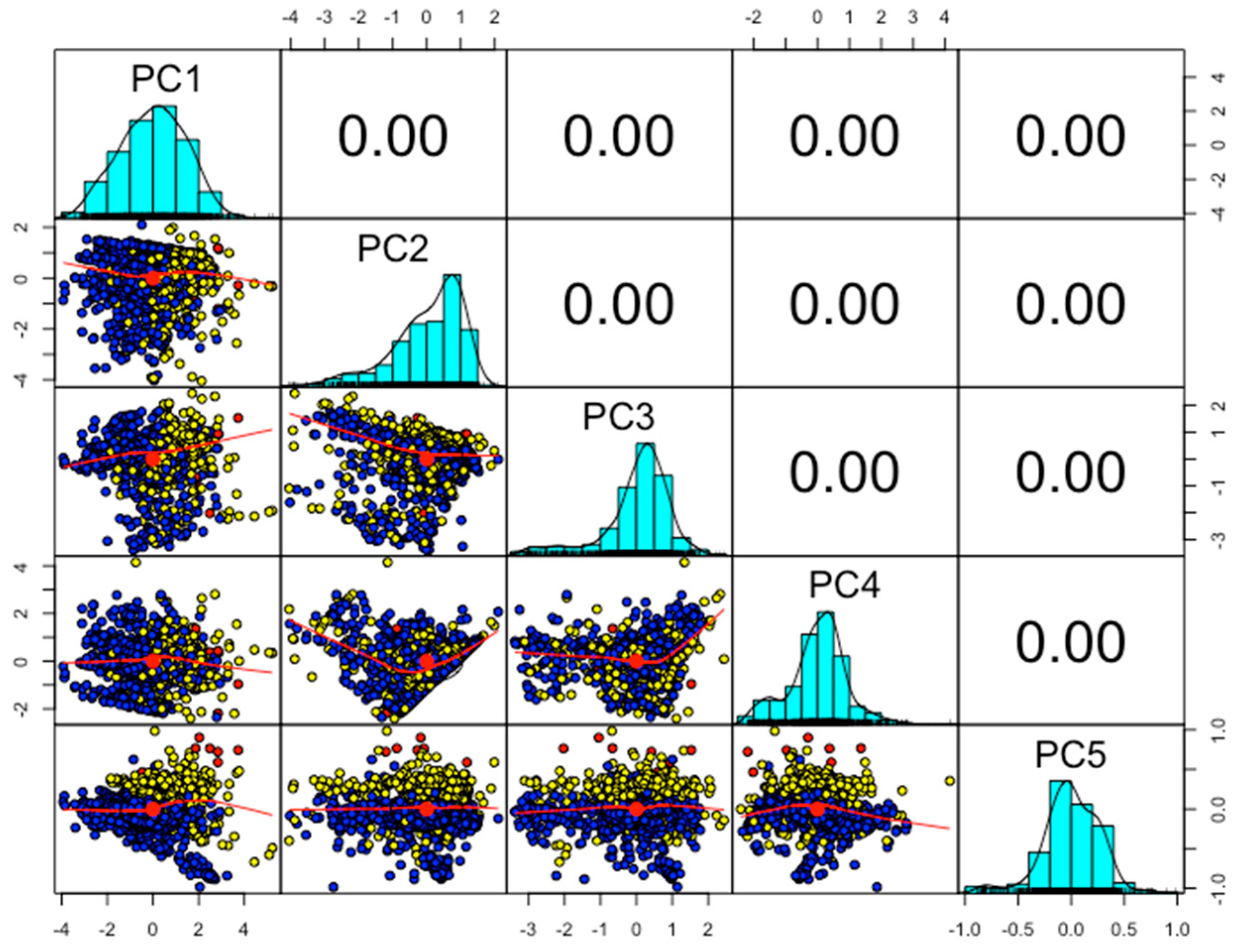
The correlation between capacity and Grid_Id is 0.01 and 0.02 between the used_area and capacity variables of the hourly wind dataset. These values are collected in different types of data with different ranges. PCA is applied to convert the various numerical values to a linear form defined with zero correlated information for hourly wind turbine data as shown in
Figure 3.
The linear combination of hourly wind turbine data is more accessible for further processing in the deep neural network. Now, the correlation values among all variables in the hourly wind data are zeros. Noise has been removed from the data and the captured features are decomposed into a reduced dimensional space. There is a total of five PCs extracted for different instances in the data, but the first three PCs capture the maximum variance. So, we used the first three PCs for the next step to apply the deep learning algorithm. The standard deviation, proportion of variance and cumulative proportion of all captured PCs are shown in
Table 1. Then, these features are used as inputs to the deep learning model. Further, it gives errors predictions and wind power forecasting for hourly, monthly and yearly wind turbine data.
3. Deep Learning with TensorFlow Framework
The principal components are then passed to the deep learning algorithm. TensorFlow is an open source machine learning-based repository that works in extensive heterogeneous and complex environments. It is used for a high level of computation, training data, sharing the state and the operations used to mutate the states by dataflow graphs. It enables presentation of computations on each node that may own or renew the mutable state in a dataflow graph. TensorFlow collects the node information from the dataflow graph in a cluster through different machines and, further, throughout numerous computational devices, for example, multicore central processing unit (CPU) and graphics processing unit (GPU). It provides a flexible environment to the application developer and allows the design of novel and optimized algorithms. It provides different types of applications for inference and to train the deep neural network. It works mainly in three steps: First, processing the data; second, designing the model; and, third, training and estimating the designed model. TensorFlow performs computations using multidimensional arrays called tensors. These are base datatypes which provide generalization of matrices and vectors. It describes the different properties of the physical system. The tensors are calculated asynchronously for the data using a queues feature. These queues work like multi-threading technology in parallel to can speed up the operation [
41,
42]. We used TensorFlow with the Keras application programming interface (API) to design a complex neural network for wind power forecasting. Keras is a high-level API that is used to train the deep learning models. It is user-friendly and used for fast prototyping and new modular extensions [
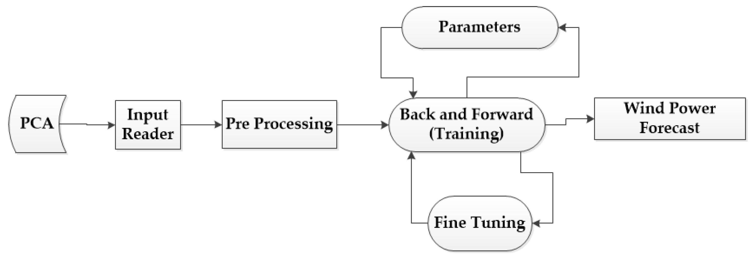
43]. The PCA data is given as an input to the TensorFlow framework. First, data is preprocessed and then queued for the training phase as shown in
Figure 4.
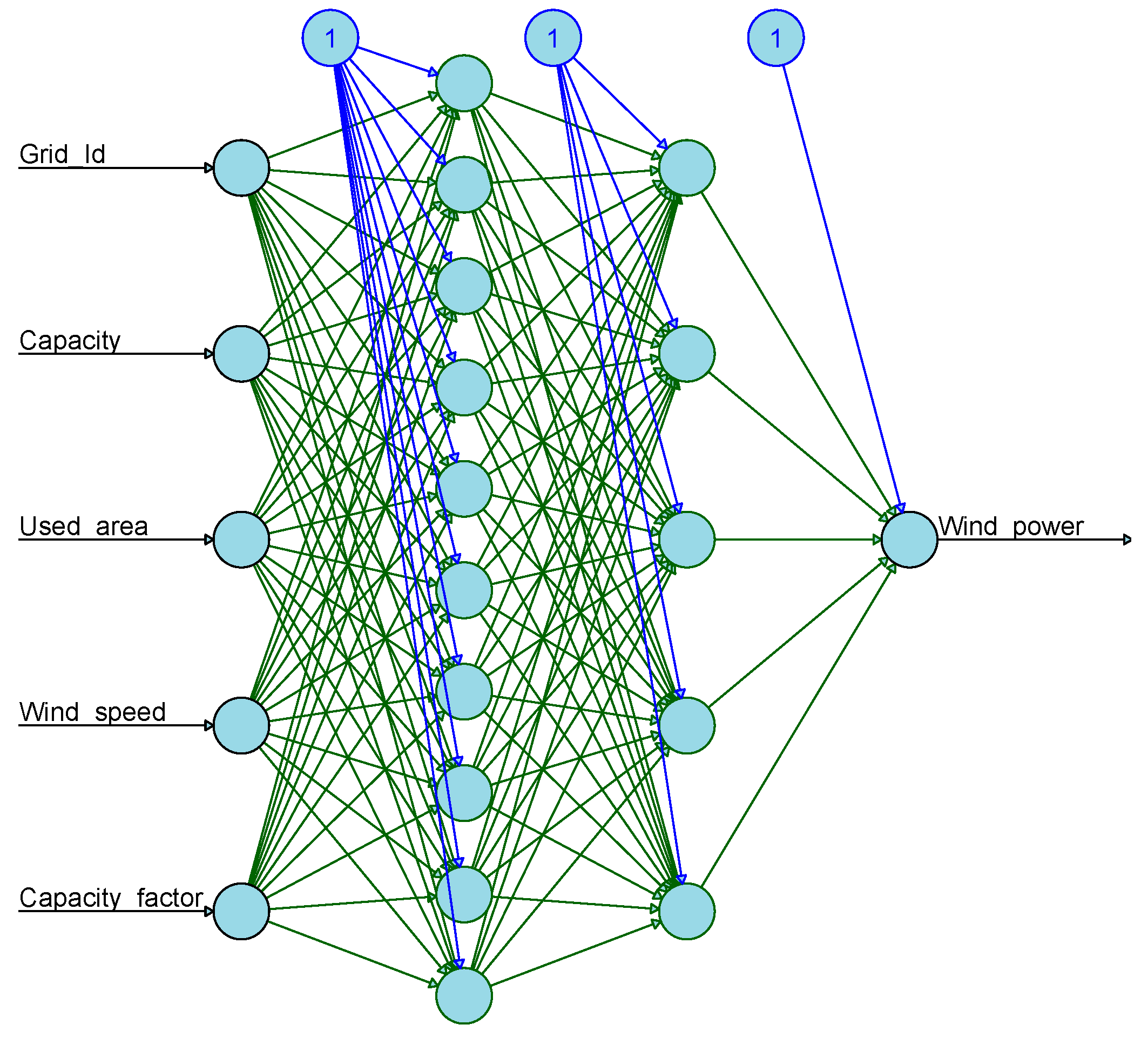
The back and forward method are used to train the threads in a loop-like process to fine tune the different parameters. The fine-tuning procedure is optimized with a different activation and loss function, dropout layer, optimizer and learning rate. This process is used to obtain better accuracy of the wind power forecast. The grid id, capacity, used area and wind speed are the input variables and the wind power forecast is the output variable. There are ten neurons in the first hidden layer and five neurons in the second hidden layer. All input values are preprocessed and trained using the TensorFlow-based deep learning framework and then wind power forecast is predicted for hourly wind turbine data as shown in
Figure 5. The sigmoid method represents the nonlinear form of the neural network model. The neural network calculates the linear arrangement of input signals and then applies a sigmoid activation function to the outcome. It is a standard logistic activation function which is used for handling multi-class problems [
44]. Mathematically it can be defined using Equation (6).
where
denotes the sigmoid function and
is the exponential function for a variable
. The entropy function is used to detect the loss to compile the deep learning model. It accepts a tensor as an input and targets the tensor with the same shape as the output. The Adam optimizer, which is also known as the stochastic descent gradient, is used for compiling and optimizing the deep learning model. It uses the iterative procedure to update the network weights and calculates the individual adaptive learning rates for each parameter in the deep learning network [
45,
46]. The decaying means of pas squared gradients are shown in Equations (7) and (8) [
47].
where
and
are the estimated means of the first and second moment gradients, respectively. The
denotes the respective gradient for each moment. It counteracts these biases by computing bias-corrected first and second-moment estimates using Equations (9) and (10) [
47].
4. Results and Discussion
The Keras API integrated with the TensorFlow framework makes it easy to turn models into products. It can be easily deployed across a wide range of platforms, i.e., iOS, Android, Google cloud, GPU-accelerated JavaScript, R or Python, etc. It does not lock the user into an eco-environment and also supports several backend engines, i.e., TensorFlow from Google, Computational Network Toolkit (CNTK) backend from Microsoft, etc. [
48]. The TensorFlow framework using the Keras API is applied to the hourly wind dataset as shown in
Table 2. Four dense layers with three corresponding dropout layers are configured in the neural network model [
49,
50]. The first layer is used to provide and specify the input shape of the wind data, and is called the input layer. The second and third layers are used to add more neurons and inference to the first input layer. These are used to get better accuracy from the designed model. The fourth layer is used for the output or target variable to analyze the possible outcomes. There are 100, 50 and 20 neurons used in the input and hidden dense layers 1, 2 and 3, respectively. Similarly, the dropout layer is used with every dense layer to solve the overfitting problem. The compile method is used to configure the learning process for each layer with loss, optimizer and metrics parameters. Further, the designed model is trained after dense layer and learning configurations. The training process is done automatically based on input shape and dense layers. The deep learning approach is used to produce its own high-quality features for complex problems and to train the features automatically in a reasonable time.
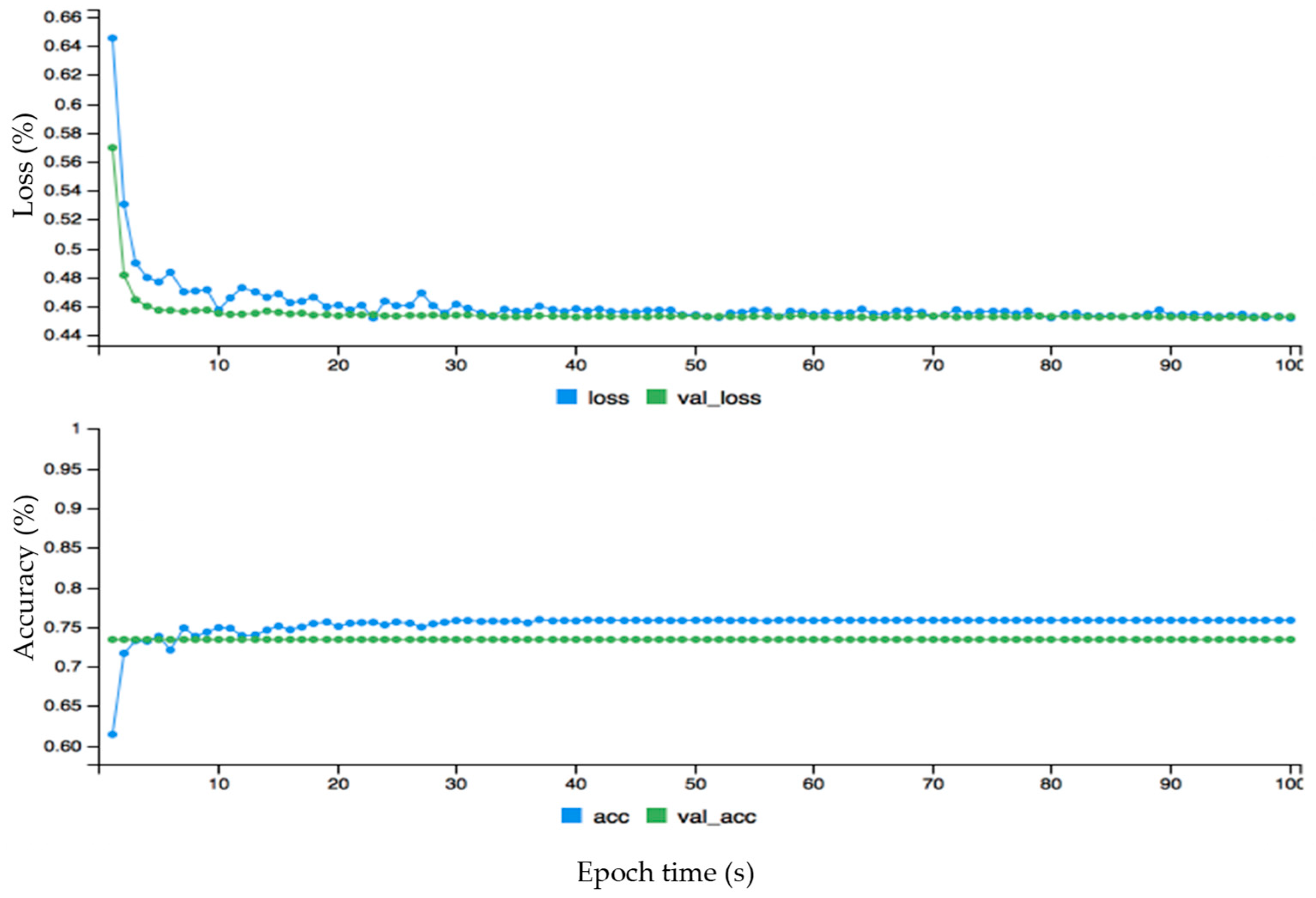
There is a total of 6733 trained parameters, of which 600 in the first layer, 5050 in the second layer and 1020 are in the third layer. The four-dense layer is used for the target variable in which 63 parameters are trained. The same methods are applied to all three datasets. The goal is to train the input variables in layers 1, 2 and 3 to target the output variable in layer 4. The model was complied with 100 epochs for loss and prediction accuracy, and the resultant dynamic graph for hourly wind data is given in
Figure 6. The epoch values are given on axis and loss, and accuracy is given on the
y-axis.
Here, acc, val_loss, val_acc represents accuracy, validation loss and validation accuracy, respectively. The loss, accuracy and loss, and validation loss are calculated for wind power forecasting. First, the loss (blue curve) is started from 0.65 and the validation loss (green curve) is started from 0.57 on the y-axis, which is a big difference between the two curves. After some time both curves behave approximately the same from around 50 on the x-axis. The fact that the loss curve is always higher than the validation of loss proves that there is no overfitting problem. This is also the case with the accuracy and validation of the accuracy graph: initially there is an overfitting problem because accuracy is lower than validation of accuracy but soon after they perform the same. The accuracy curve is above the validation of accuracy, proving that there is no overfitting problem. The dynamic forecasting plot of the monthly wind data before fine-tuning error configuration is given in
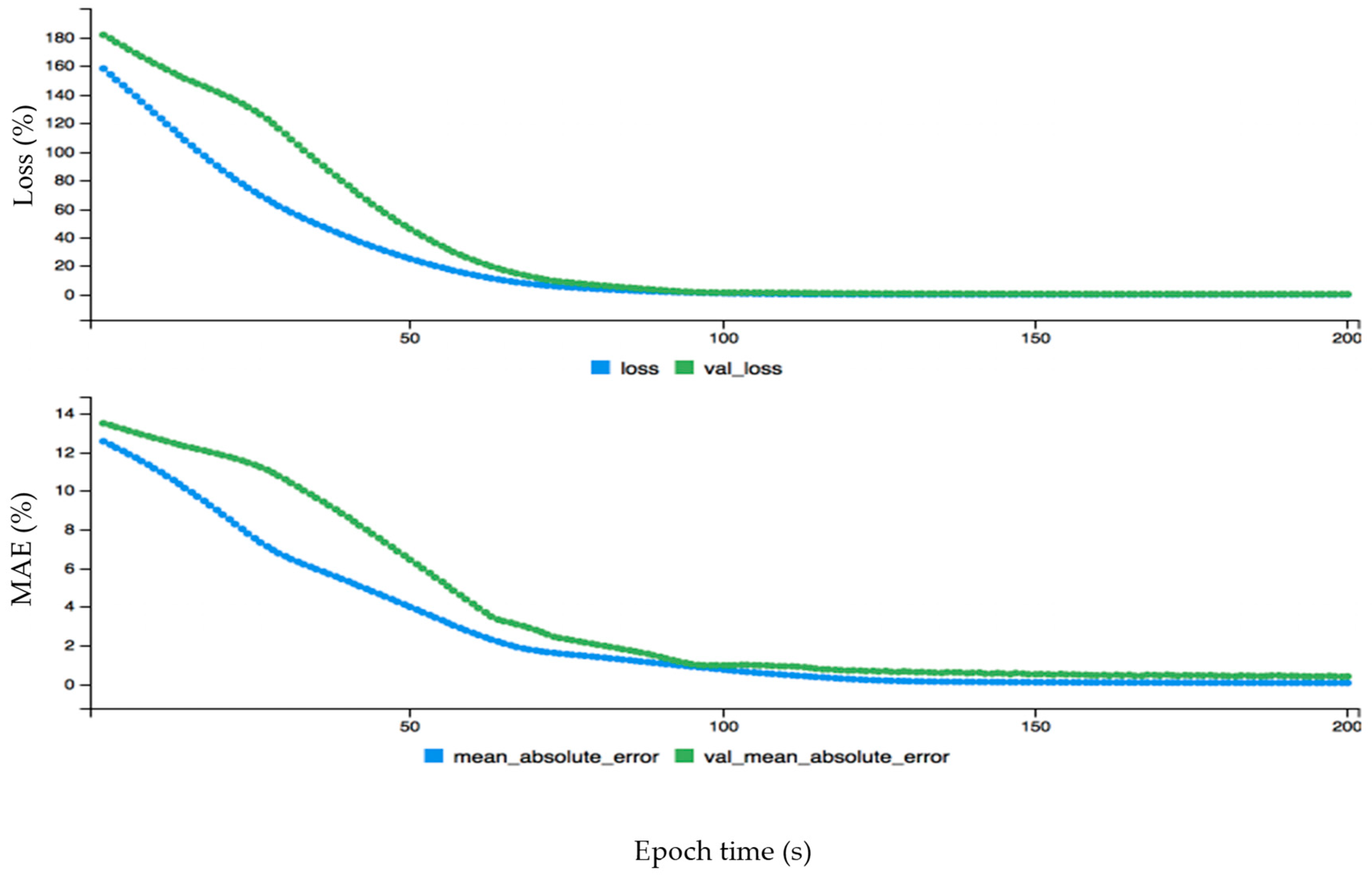
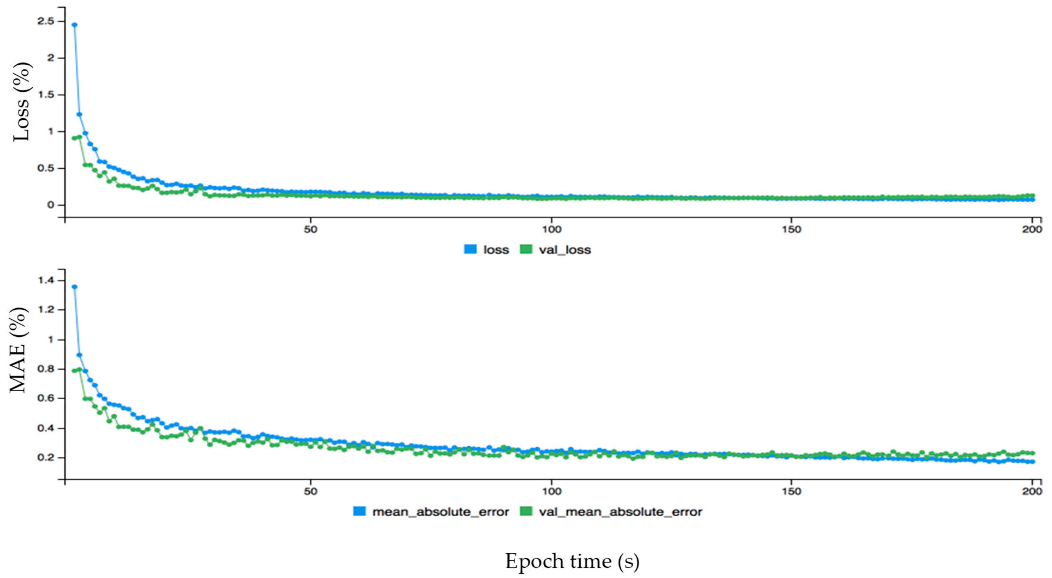
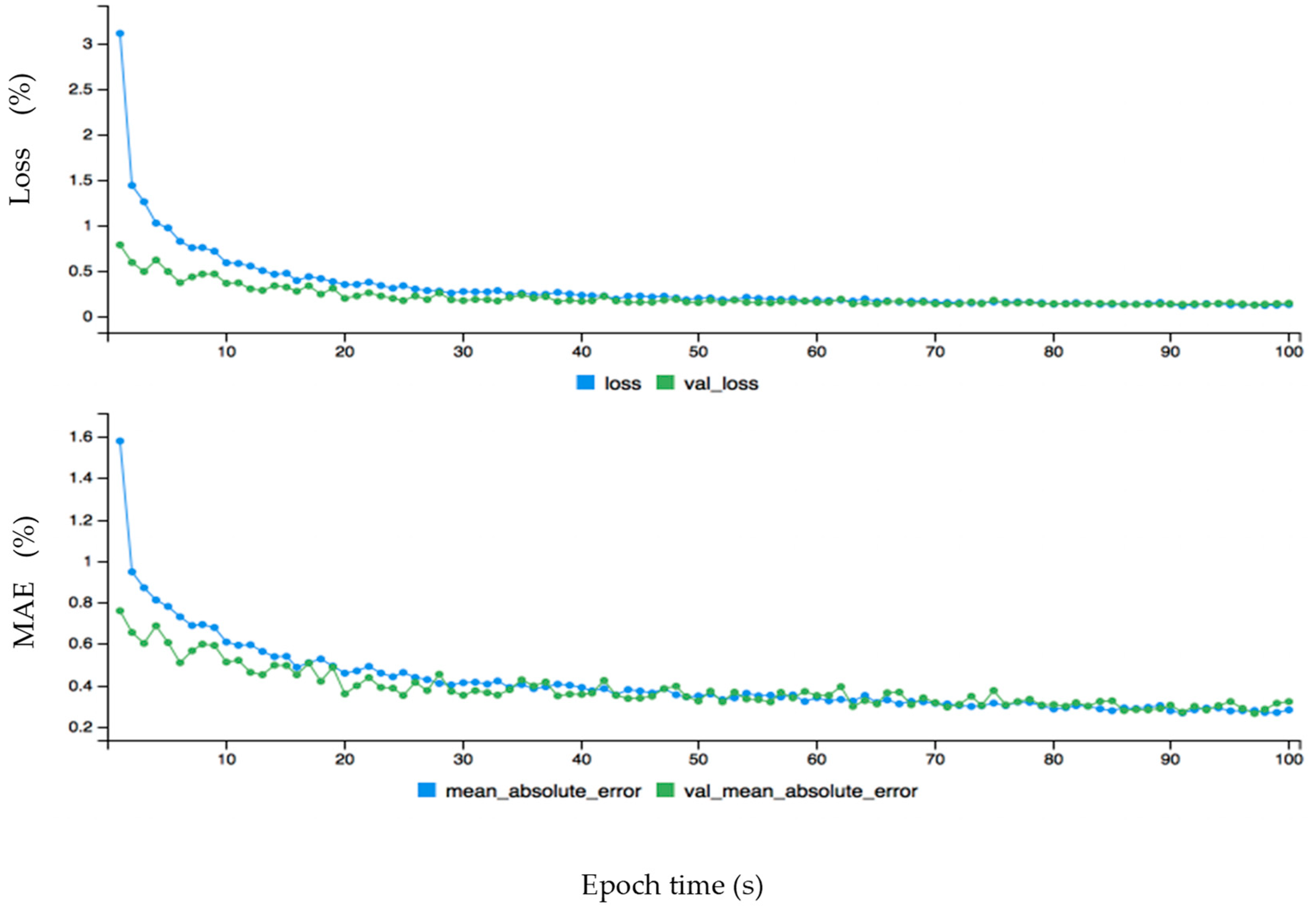
Figure 7. The data is fine-tuned dynamically for monthly wind data to get better results as shown in
Figure 8. The epoch values are given on the x-axis, and loss and mean absolute error are given on the y-axis. First, both curves started from different ranges on the y-axis, but soon after are flowing in the same direction. The loss curve is above the validation loss, proving there is no overfitting problem. The mean absolute error is lower than the validated mean absolute error, which also confirms that there is no problem of overfitting. The mean absolute error (MAE) for monthly wind power prediction is calculated and checked for the loss and errors on each point of the cycle. It is shown that is there an overfitting problem that affects the overall accuracy for monthly wind power forecasting. Similarly, the hourly and annual wind turbine data are analyzed before and after fine tuning error configuration as shown in
Figure 9,
Figure 10,
Figure 11 and
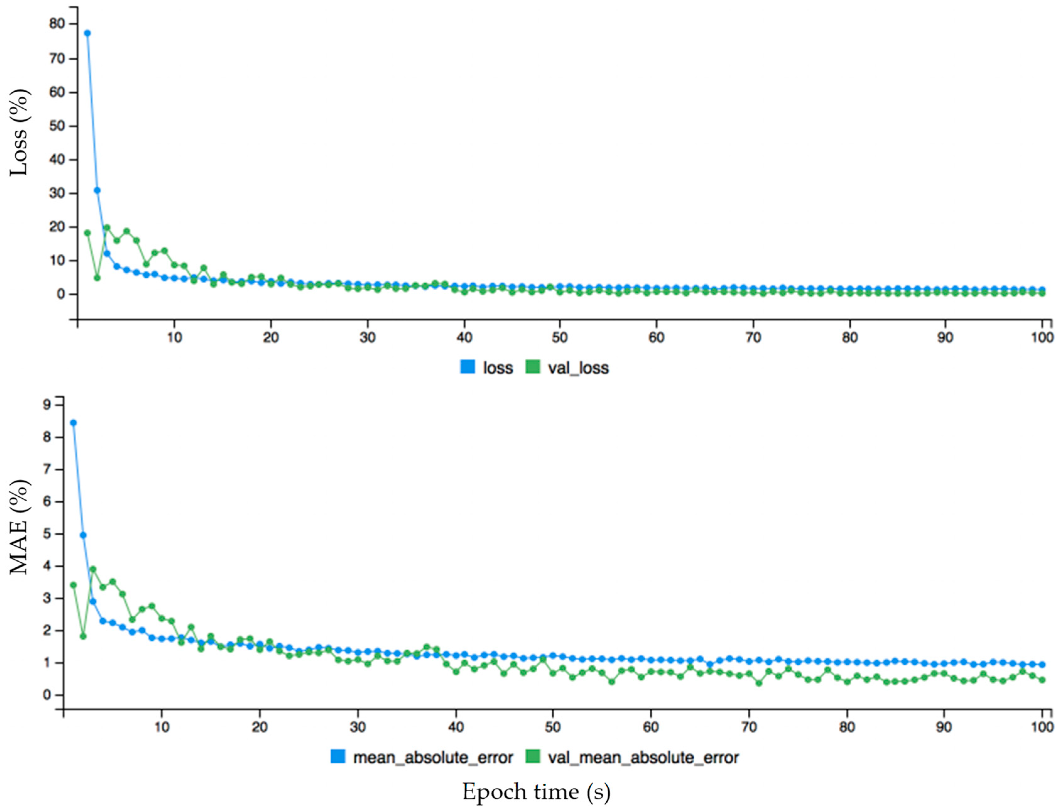
Figure 12, respectively.
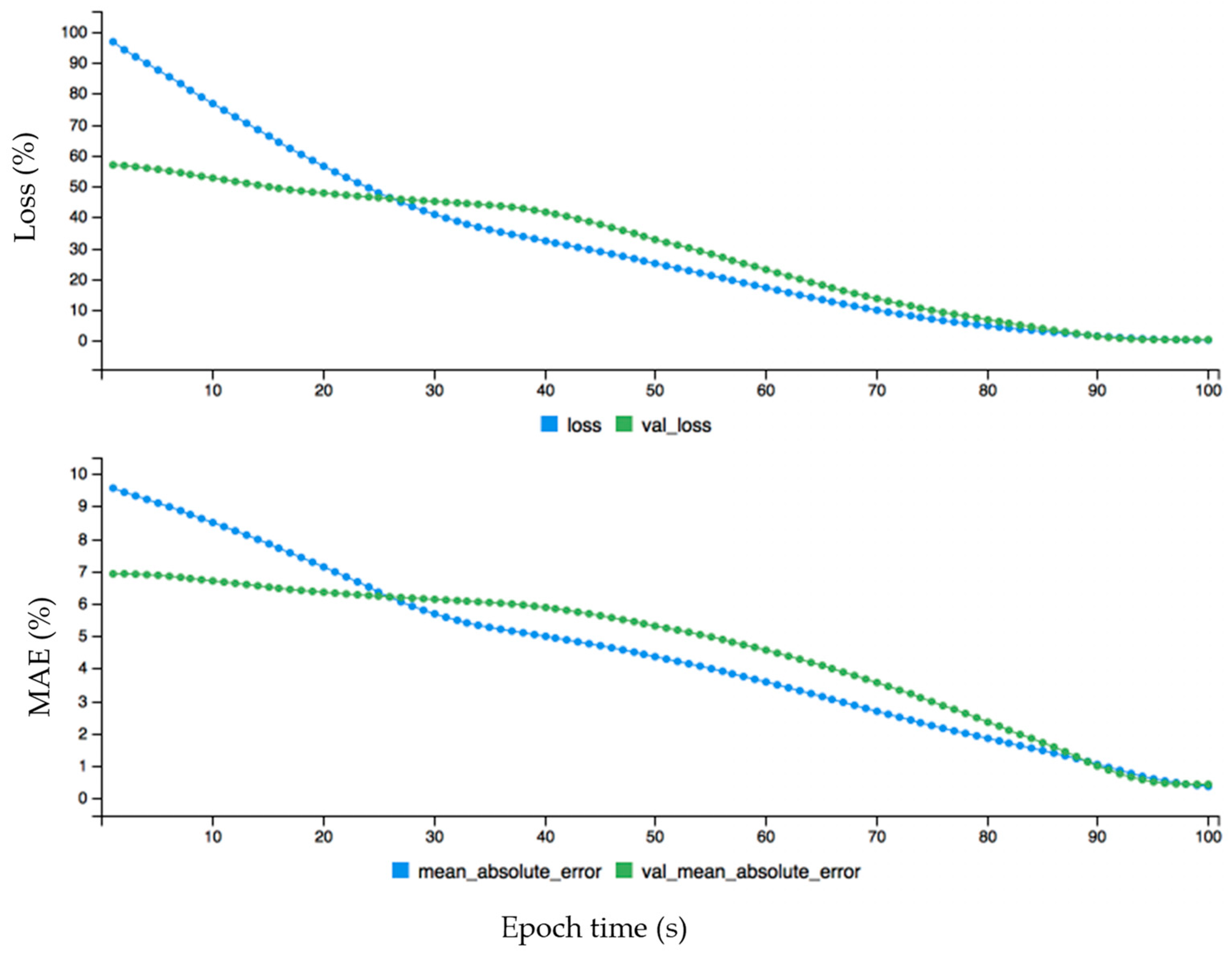
Overall, the yearly wind data behave very differently compared to hourly and monthly data. A big difference is shown between the loss and validation curves without fine tuning configuration. The loss curve starts from 100 while validation loss starts from 60, which shows an overfitting problem, and approximately on the 25 epoch it shows the opposite performance. After fine-tuning configuration, at approximately the 3 epoch it acts normally and without an overfitting problem. Further, the performance of the proposed model is evaluated by comparing the actual and predicted data. The hourly wind data instances are analyzed to find which data instances are predicted and which or not. If the diagonal line grows in a linear form, then it shows the correct prediction of each data instance of the hourly data. The performance evaluation test of the proposed approach for hourly wind data before fine-tuning error configuration is shown in
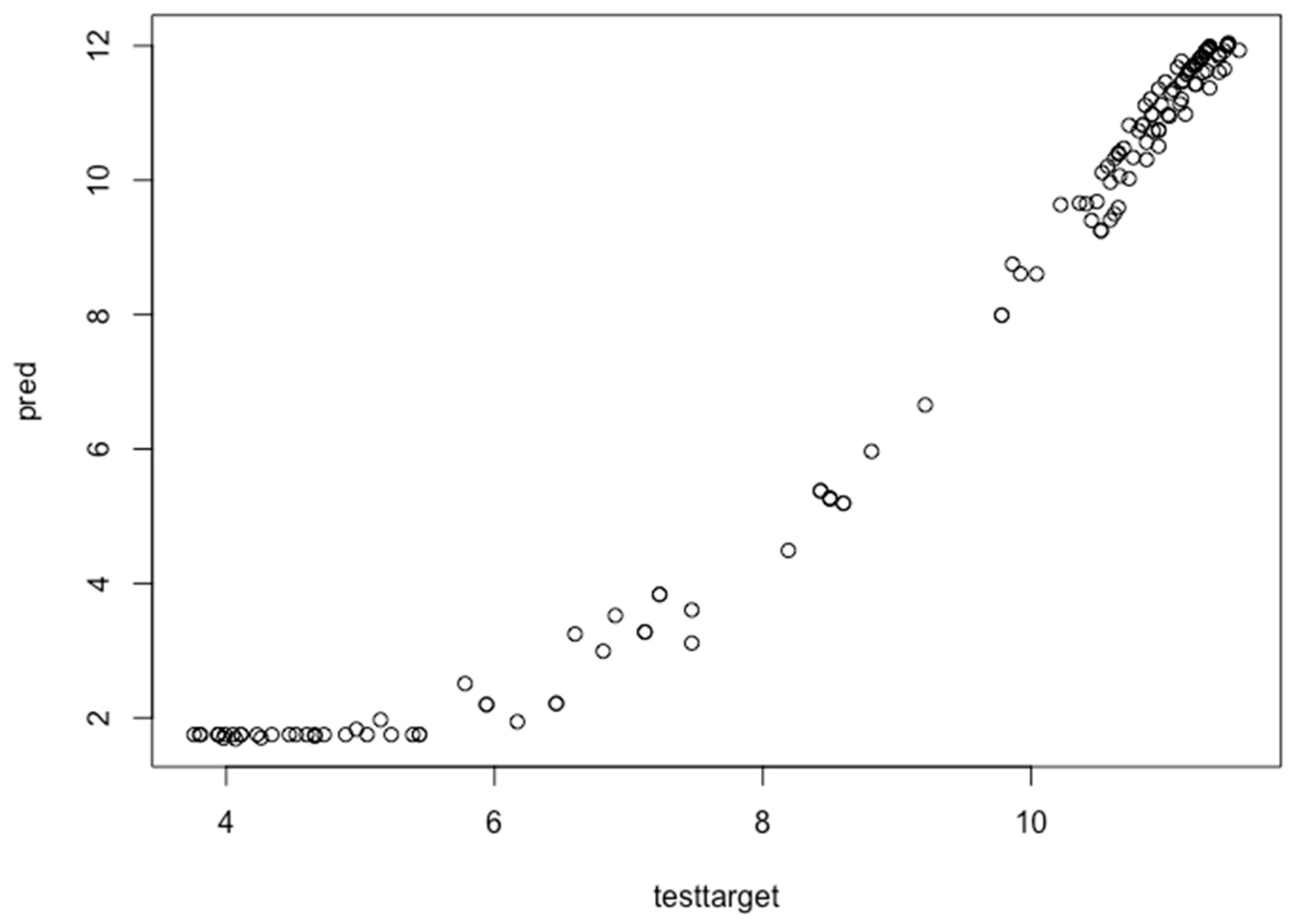
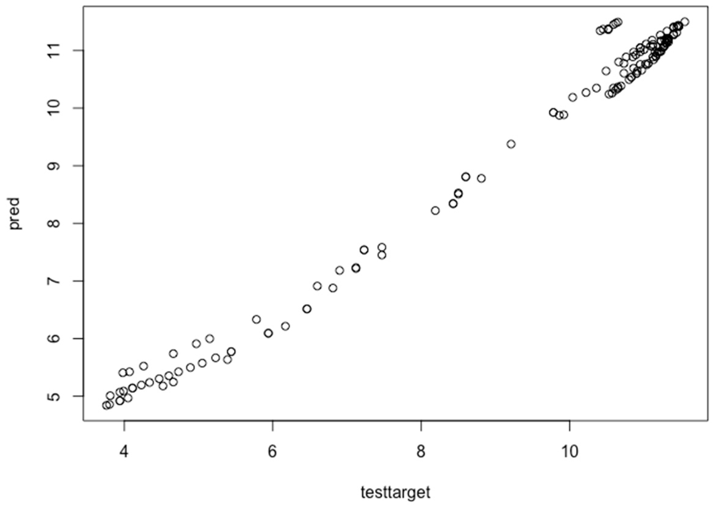
Figure 13. First, the wind turbine data is divided into training and testing data sets. The training data is required to train the data, and once the model is developed, then the testing set is used to check the performance of the model predictions. The test target represents the actual data and pred represents the predicted data. It shows the performance evaluation test of the proposed deep learning approach with the test and test targeted data instances. The test target is given on the x-axis, and the predicted values are given on the y-axis.
The black circles represent the relationship between the actual data (testtarget) and the predicted data (pred). First, the curve increases on the x-axis up to 6 epochs, but after switches to the y-axis. The graph is not in a linear form, and it needs fine-tuning configuration to predict the wind forecast accurately and to remove the overfitting. The fine-tuned chart for hourly wind turbine data is shown in
Figure 14.
Again, the performance evaluation is tested for each data instance in the hourly wind dataset. The actual data are given on the x-axis and the predicted data are provided on the y-axis. The fine-tuned graph has a more linear form than the previous data graph. The same process is followed for all three wind turbine datasets. Further, the designed model is fine-tuned to get the optimal values of MAE and root mean square error (RMSE). The learning error rate, optimization function, activation function and loss parameters are used to fine-tune the deep learning model [
51]. The MAE and RMSE values are 0.150388656, 0.055307715, respectively, for the hourly wind dataset, 0.07624394, 0.07360119, respectively, for the monthly wind dataset and 0.2752635, 0.1485754, respectively, for the yearly dataset. Mathematically, the MAE and RMSE are given in Equations (11) and (12), respectively [
52,
53]. The MAE is the mean value between two coordinates.
where
and
are two coordinates and
is the number of data points occurring between these two coordinates. The RMSE is the root of the cumulative differences between two values or samples. The first value is the predicted value and the second is the observed value.
where
is the predicted value,
is the observed value and
is the total number of values or samples. The predicted wind power errors are compared with the popular state of the art algorithms, i.e., BPNN, SVM, ensemble selection with back and forward procedure, CNN and AR. The comparison of MAE and RMSE errors for hourly, monthly and yearly wind turbine datasets is shown in
Table 3. In hourly results the MAE and RMSE are better than the others. Similarly, the MAE and RMSE for the monthly wind dataset yielded better results than other approaches. Further, for the yearly wind dataset, the ensemble selection for MAE gave slightly better results than the proposed approach for yearly data. Overall, it is shown that our proposed approach has better accuracy compared to other methods.
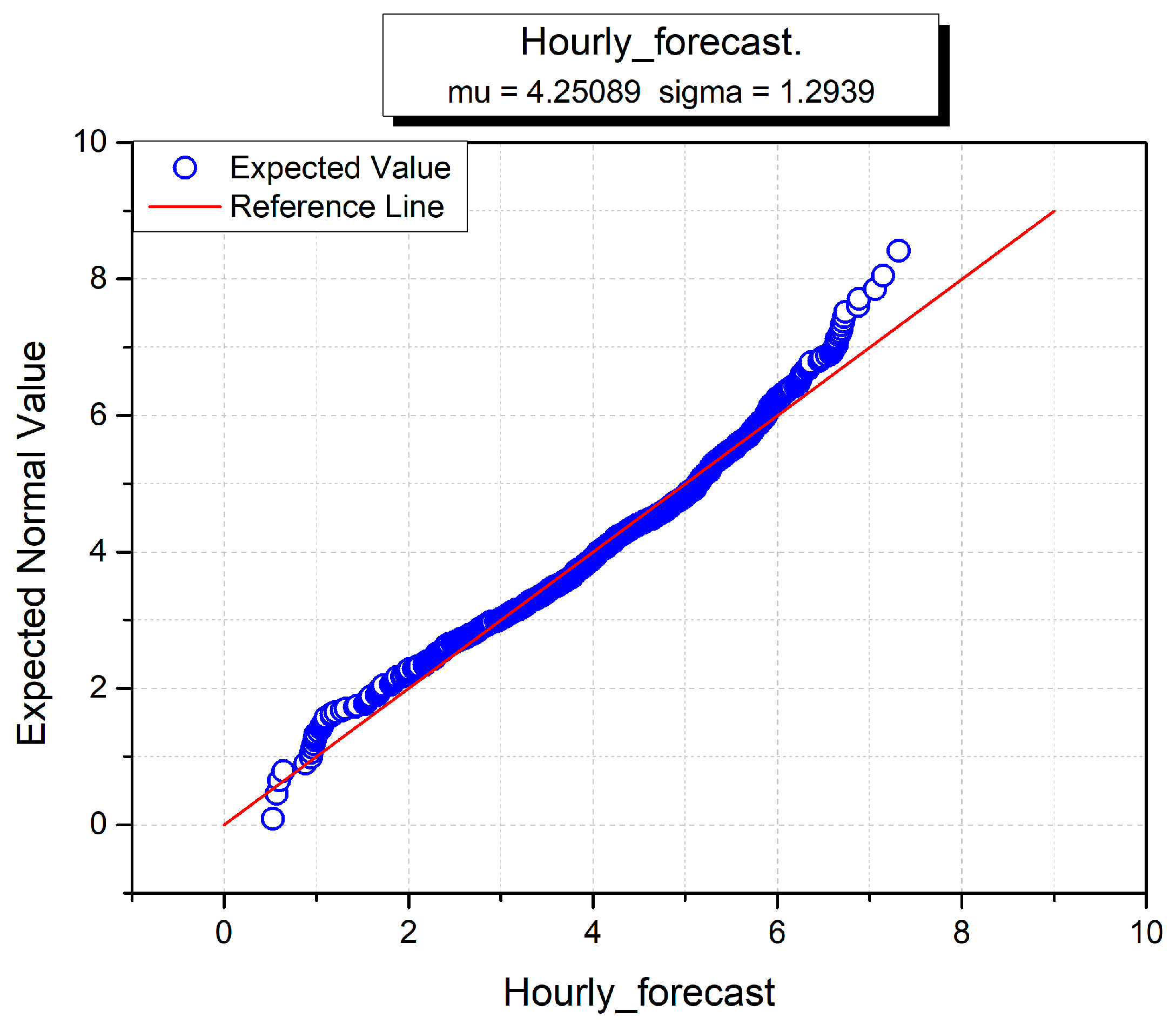
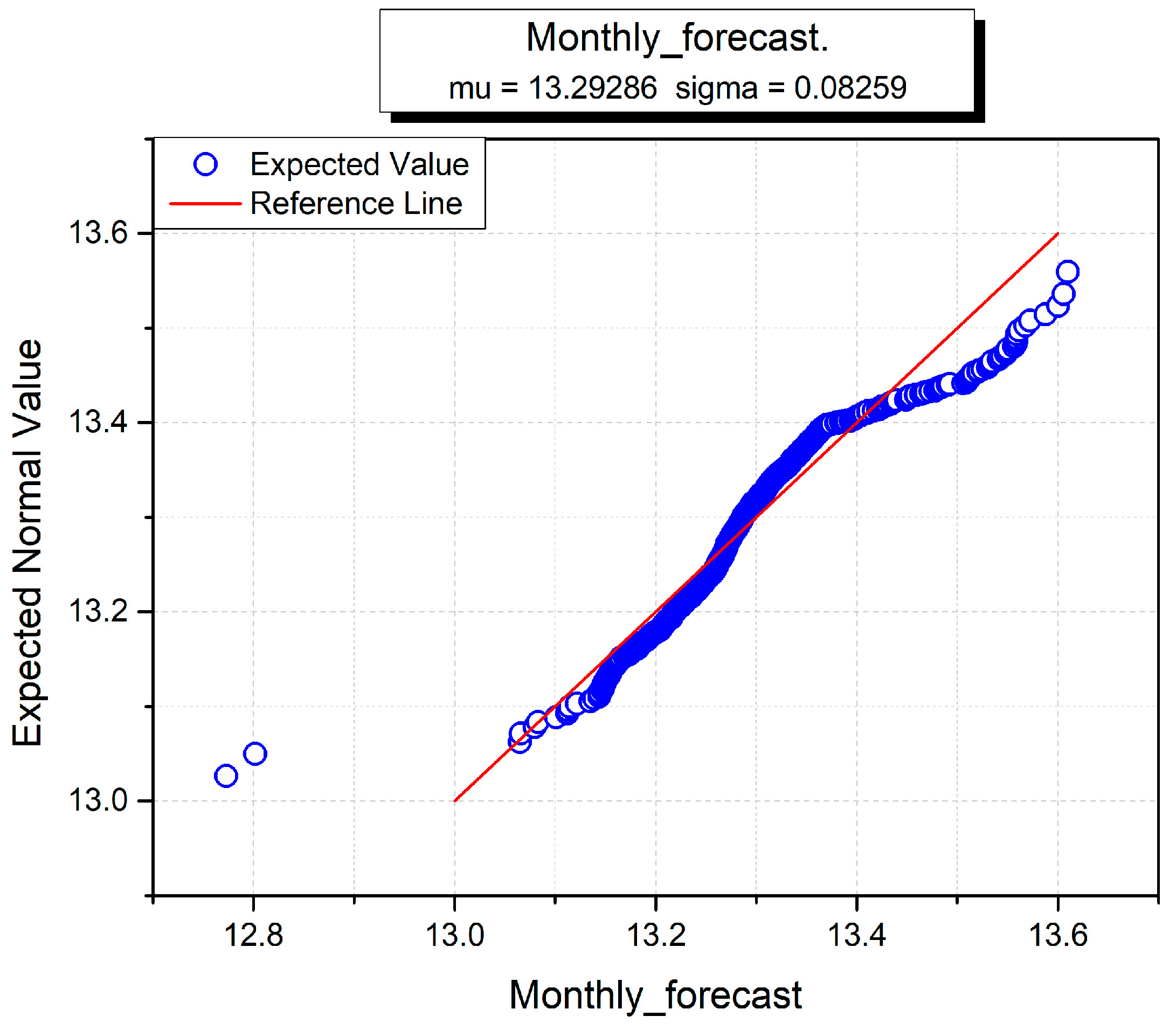
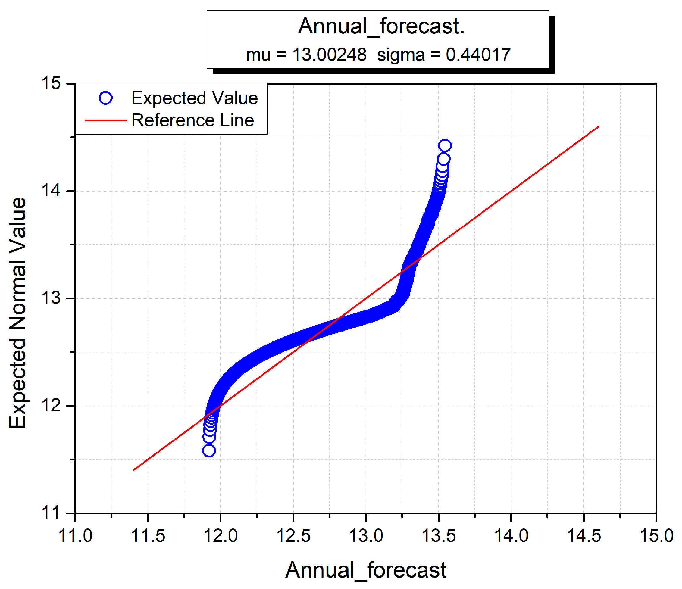
The hourly, monthly and yearly wind turbine data for forecasting wind power are given in
Figure 15,
Figure 16 and
Figure 17. The sigma (standard deviation) and mu (mean) are used to analyze the normal distributions of all input variables against the hourly forecast, monthly forecast and yearly forecast predictions [
54]. In all three figures, hourly, monthly and annual forecasts are given, and the estimated normal distributions are shown on the y-axis. It is used to test the distribution and normality of data instances of individual datasets. The red line shows the standard normal form and the blue line conforms to the data instance in all three figures. The sigma and mu standard functions are used to investigate the normal distribution of each wind dataset. The blue curve indicates the corresponding wind turbine data, and the linear red line shows the standard normal distribution against the x-axis. At the start, the hourly curve behaves better than the monthly and yearly curves, but soon after takes a nonlinear form against the standard distribution. Overall, the annual curve performs worse than the other two curves because it neither starts nor ends towards the standard distribution line. The monthly curve is better than the others, which demonstrates that monthly wind power prediction accuracy is greater than fir the other two datasets.
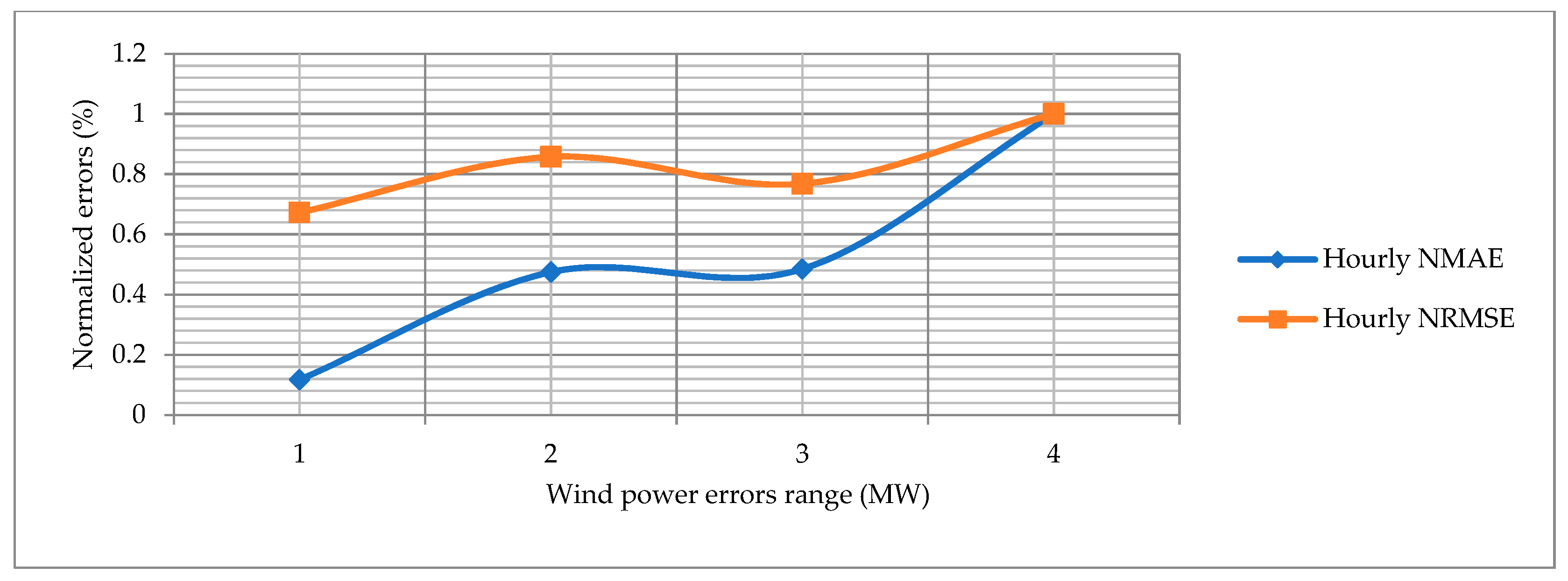
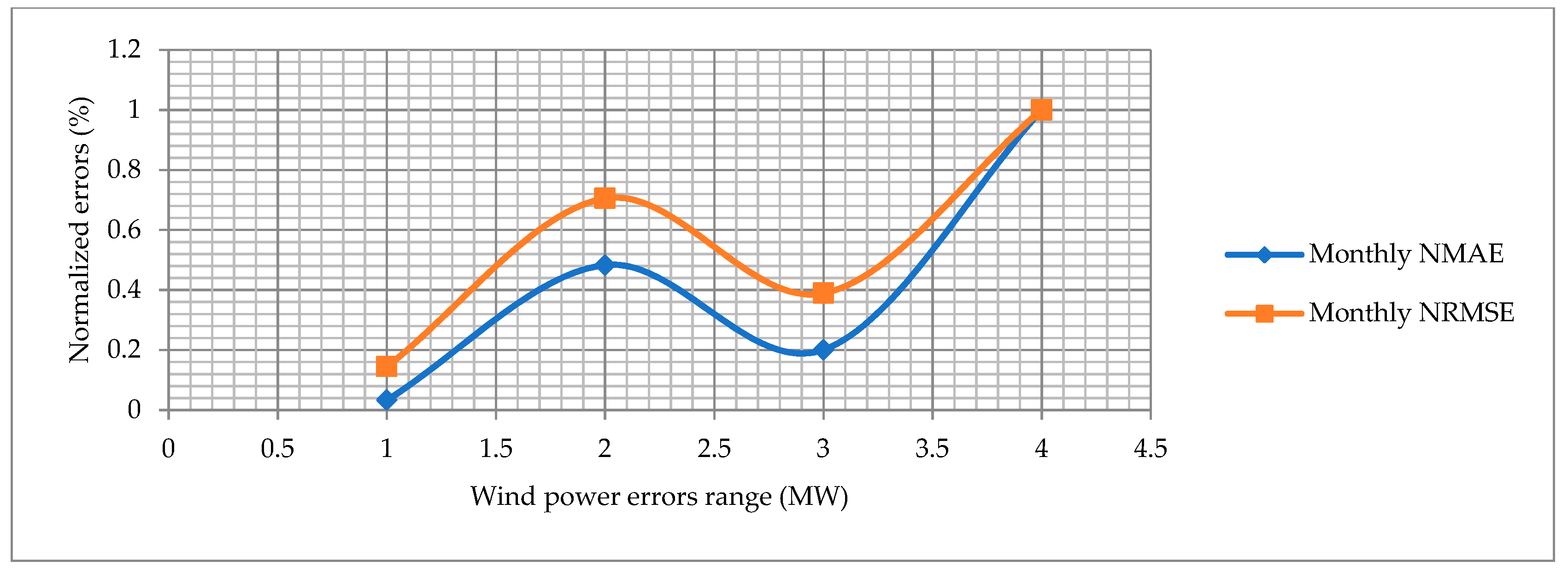
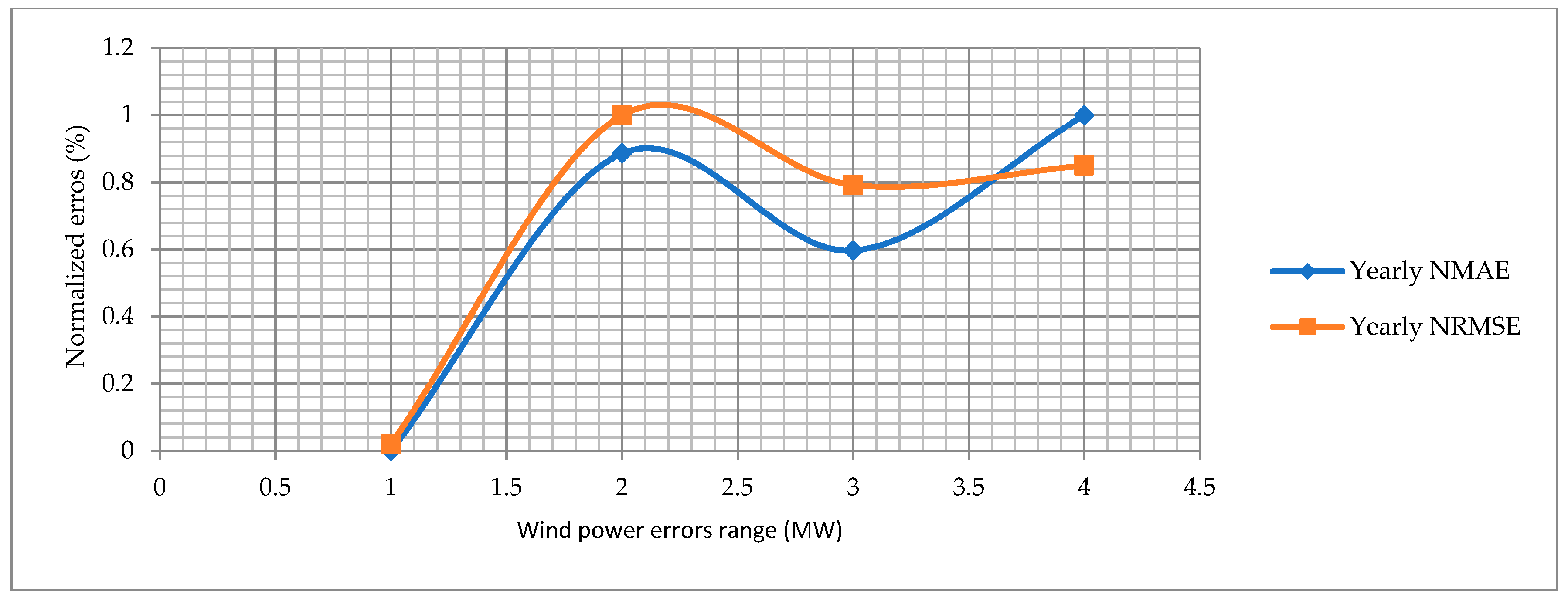
The normalized mean absolute error (NMAE) and normalized root mean square error (NRMSE) are calculated for the proposed approach and other state-of-the-art algorithms. The RMAE and NRMSE for the hourly, monthly and yearly wind power forecast graphs are shown in
Figure 18,
Figure 19 and
Figure 20. The blue line shows the normalized NMAE and the orange line shows the NRMSE. The normalized errors are calculated in a range of 0 to 1 on the y-axis. The wind power error range is different in each figure, which indicates the minimum and maximum limit of each wind power error on the x-axis. The NRMSE is always higher than the RMSE, which indicates that the wind power forecasting errors are precise and accurate. Overall, the hourly normalized errors behave the same because both curves almost have the same direction. Secondly, the normalized errors for the monthly wind power forecasting perform better.
5. Conclusions
A new hybrid approach using PCA with a deep learning neural network is designed to forecast wind power. The proposed deep learning approach implemented the TensorFlow framework with the Keras API. The proposed research is examined on large scale wind turbine data gathered with a duration of 17 years. Three datasets are obtained from NREL (US), namely, hourly, monthly and yearly wind turbine data. First, PCA is applied to all three datasets to mine hidden information and focus on meaningful patterns in reduced dimensional space, yielding data in a normalized form with principal components. Then, a few PCs are selected for a deep learning experiment which contains high variance of the data. The proposed deep learning algorithm is applied to PCs to forecast wind power. The Keras API is used with TensorFlow to configure a more reliable neural network. Further, the proposed algorithm is fine-tuned for the trained parameters in terms of learning error rate, dense and dropout layers, loss and activation function, and several hidden neurons are used in each hidden layer. The fine-tuned configuration removed the overfitting problem and increased accuracy. The MAE and RMSE are calculated for the proposed research and, then, the corresponding errors are estimated to forecast wind power. The results are compared with the existing methods, and it is verified that the proposed hybrid approach outperforms. The fine tuning configuration has a wide scope for research, and can affect the results in a positive way. Our proposed TensorFlow deep learning approach has the following benefits over other state-of-the-art techniques, as follows.
It gives better visualization and computations for large-scale and real-time data collected from wind farms.
TensorFlow integrates various APIs that are used to design deep learning architectures for large scales of data, i.e., the GitHub framework.
Dense layer: we may configure input and output dense layers by our own selected activation functions, number of neurons, input and output shapes.
Overfitting: The dropout layer is used to resolve the overfitting problem in the data and to provide better accuracy for large scales of wind data. We may optimize the dropout layer by fine tuning configuration, i.e., learning error rate, loss and activation function.
It trains the wind data automatically by fitting the model.
We may get better accuracy by increasing the number of dense layers, the number of neurons and a dropout layer in fine tuning control configuration
It can be deployed in a range from cellular machines to large complex networks. It offers seamless performance and quick updates, as it is supported by a big company, i.e., Google.
In the future, we will work to optimize the fine tuning of other parameters with extensive analysis compared to the existing methods. The activation and loss function, dropout layer, number of neurons in each hidden layer and the learning error rate can be enhanced to get better results. The proposed deep learning methodology can be deployed on the physical infrastructure of wind turbines data. This needs the wind turbines’ historical data as an input and, after, will display the future wind power forecast with minimum error predictions.


