Kick Risk Forecasting and Evaluating During Drilling Based on Autoregressive Integrated Moving Average Model


1
School of Oil & Natural Gas Engineering, Southwest Petroleum University, Chengdu 610500, China
2
Industrial Systems Engineering, University of Regina, Regina, SK S4S0A2, Canada
*
Authors to whom correspondence should be addressed.
Energies 2019, 12(18), 3540; https://0-doi-org.brum.beds.ac.uk/10.3390/en12183540
Submission received: 30 July 2019
/
Revised: 5 September 2019
/
Accepted: 13 September 2019
/
Published: 16 September 2019
(This article belongs to the Special Issue Data Analytics in Energy Systems)
Abstract
:Timely forecasting of the kick risk after a well kick can reduce the waiting time after well shut-in and provide more time for well killing operations. At present, the multiphase flow model is used to simulate and forecast the pit gain and casing pressure. Due to the complexity of downhole conditions, calculation of the multiphase flow model is difficult. In this paper, the time series analysis method is used to excavate the information contained in the time-varying data of pit gain and casing pressure. A forecasting model based on a time series analysis method of pit gain and casing pressure is established to forecast the pit gain and casing pressure after a kick. To divide the kick risk level and achieve the forecasting of the kick risk before and after well shut-in, kick risk analysis plates based on pit gain and casing pressure are established. Three pit gain cases and one casing pressure case are studied, and a comparison between measured data and predicted data shows that the proposed method has high prediction accuracy and repeatability.
1. Introduction
During drilling operation, a permanent concern is kick risk forecasting and well control. A kick is defined as the uncontrolled influx of formation fluid or gas into the wellbore, which occurs when the wellbore pressure at a certain location is less than the formation pressure, and requires a well control emergency plan [1]. Influx fluids tend to have a high pressure; a gas kick is much more detrimental than a liquid kick due to gas expansion and, as a result, has a higher variation in pressure. Late kick detection and risk forecast increase the amount of formation fluid that enters the well borehole, which increases the kick pressure and makes it hard to control the kick and can even lead to an uncontrolled blowout. For well control safety, it is necessary to forecast the risk of a kick to reduce the shut-in time of a well and provide more time for the killing operation.
As a kick can pose a significant threat to safety drilling, a lot of work has been devoted to detecting kicks. Nowadays, kick-detection methods have developed from simple thresholding methods [2] into complex intelligent methods based on machine learning [3,4,5,6,7,8,9,10]. Sun et al. [3] proposed one integrated pattern-recognition model consisting of a dynamic multiphase wellbore flow model and improved the piecewise approximation and similarity measure algorithms for kick diagnosis. P. Andia and R. R. Israel [4] utilized a cyber-physical approach that combined physics-based modeling with Bayesian mathematics for detecting a kick. Shi et al. [5] adopted the random forest and support vector machine algorithms to detect a kick during drilling in real-time. Alouhali et al. [6] trained and evaluated five models—Decision Tree, K-Nearest Neighbor (KNN), Sequential Minimal Optimization (SMO) Algorithm, Artificial Neural Network (ANN), and Bayesian Network—to detect kicks based on actual kick cases. The Decision Tree and K-Nearest Neighbor were shown to be slightly more accurate than the others. Hargreaves et al. [7] used a Bayesian probabilistic framework to detect a kick early based on noisy drilling data. Pournazari et al. [8] proposed a pattern-recognition system based on Symbolic Aggregate Approximation (SAX) to identify a kick. Unrau et al. [9] undertook modern machine learning techniques to reduce false kick alarm rates while increasing the probability of kick detection. Brakel J et al. [10] applied modern noise reduction and pattern-recognition signal processing to produce earlier and more informative kick-detection notification. However, their work was mainly done to detect a kick, whether or not by machine learning, not to predict the development trend of kick risk.
Once a kick occurs, the first thing to do is to decide whether and when to close the well. According to specifications for well control technology in oil and gas drilling by the Sinopec Group, an alarm should be triggered when the pit gain is 2 m3, and the well should be closed when the pit gain is 3 m3. As pit gain can indirectly reflect the volume and rate of formation fluid intrusion into the wellbore, pit gain can be treated as an important indicator of kick risk before well shut-in. Once the well is shut in, the casing annulus pressure will rise because of the wellbore afterflow and gas slippage, thus, casing pressure can be treated as the indicator of kick risk after well shut-in. Therefore, the kick risk can be forecasted through forecasting the pit gain before well shut-in and the casing pressure after well shut-in.
At present, as it was in the past, gas–liquid two-phase fluid dynamics is the main method used by scholars to simulate and forecast kick parameters before and after well shut-in. John Billingham [11] considered the influences of wellbore afterflow and slippage and simulated and analyzed the change in wellbore pressure during shut-in by using a continuous gas column model. Avelar et al. [12], Gao et al. [13], and Sun et al. [14] used gas–liquid two-phase flow to simulate the overflow and wellbore pressure distribution in deepwater drilling. Ren et al. [15] established a gas–liquid two-phase flow model to determine the gas invasion velocity and location during drilling by using the relationship between the standpipe pressure and the gas invasion velocity and height. Aarsnes et al. [16] and Meng et al. [17] used a transient two-phase flow model to simulate and predict the annulus pressure profile in the gas invasion into the wellbore. Based on percolation mechanics and gas–liquid two-phase flow, Ren et al. [18] considered the wellbore afterflow effect and gas slippage effect to simulate the bottom hole pressure during shut-in. Due to the laws of formation fluid invading the wellbore and those of the multiphase fluid flow in the wellbore being very complex when kick occurs, it is difficult to describe the physical process accurately using a mathematical model. Considering the difficulty and efficiency of calculation, the wellbore flow model can be simplified, resulting in a reduction in the accuracy of prediction. Besides, because of the complex downhole conditions, it is difficult to determine the intrusion rate of formation fluid and the distribution of gas–liquid two-phase in the wellbore accurately at the initial time. Empirical formulas or hypothetical methods are usually used, so the initial and boundary conditions do not reflect the actual annulus situation of the wellbore, thus reducing the prediction accuracy.
An alternative method is to construct a prediction model based on the parameters themselves and to use the already measured parameters to predict the subsequent parameters. For the prediction of short-term and medium-term time-varying parameters, the time series analysis method (e.g.; ARIMA) can reveal the development laws of the time series from the autocorrelation point of the parameters and has the advantage of having a high fitting degree [19,20]. Characteristic parameters, such as the pit gain and casing pressure, change regularly with time in a short period. Therefore, this method can extract the feature information in a short time, mine the valuable information hidden in the historical data in a short time, and construct the time series prediction model of pit gain and casing pressure to predict the pit gain and casing pressure after a kick. Time series analysis methods are widely used in the field of petroleum prediction, such as crude oil price fluctuations [21], drilling site risk probability prediction [22], oil and gas well production prediction [23,24], but they are not applied in the prediction of kick risk. Therefore, this paper uses the summation autoregressive moving average model (ARIMA) to predict pit gain before shut-in and casing pressure after shut-in and uses the predicted values of pit gain and casing pressure to analyze the kick risk before and after shut-in.
2. Mathematical Models
In the field of statistics, a set of random variables arranged in chronological order (X1, X2, …, Xt, …) is often used to represent the time series of a random event, denoted as {Xt, tT}. The n ordered observations of the series are represented by {xt, t = 1, 2,..., n}, referred to as the series of observations of series length n. The purpose of studying time series is to reveal the properties of a random time series {Xt}. To get the properties of a random time series {Xt}, we need to analyze the properties of its observation series {xt} and infer the properties of the random time series {Xt} from the properties of the observation series [25].
As the series of kick characterization parameters, such as the pit gain or casing pressure, are mostly a non-stationary time series, the autoregressive moving average model (ARIMA) is the most suitable [26]. The expression of ARIMA (p,d,q) is
where is the observation series, is the autoregressive coefficient, is the random interference series, is the mean value, is the variance, is the delay operator, d is the differential order, is the autoregressive coefficient polynomial for the stationary reversible ARMA (p,q) model, and is the moving smoothing coefficient polynomial for the stationary reversible ARMA (p,q) model.
3. Methodology
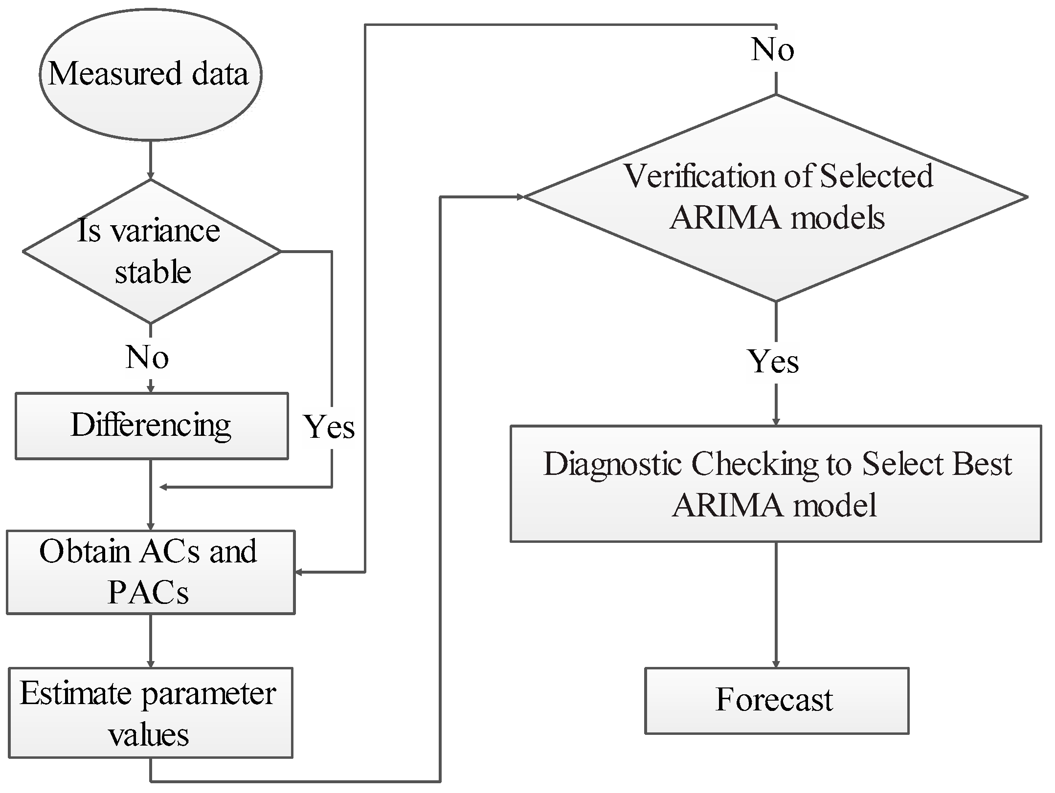
The steps to establish the model are as follows (Figure 1):
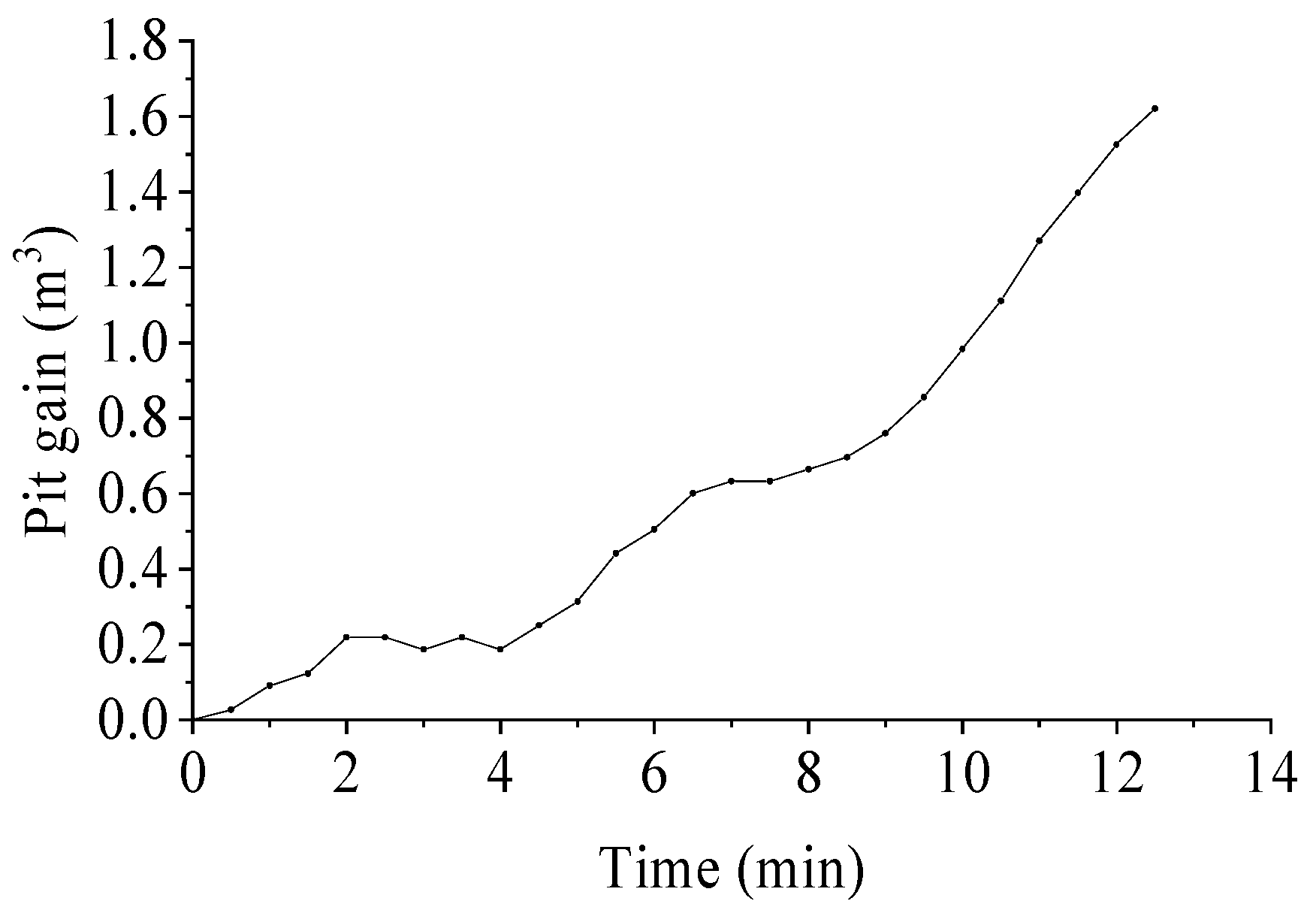
A gas well named SC-X1 in Sichuan Basin encountered a gas kick during the drilling of the gas zone. Figure 2 is a time sequence diagram of the measured pit gain data before well shut-in. This is used to introduce how to use this methodology in combination with the theoretical model.
3.1. Stationarity Test of Parameter Series
There are three main methods that test the stability of the parameter series—the time series diagram test, the autocorrelation diagram test, and the unit root test [27]:
3.1.1. Time Series Diagram Test
For a stationary parametric time series, the series’ mean and variance are constant, so the sequence shown in the sequence diagram fluctuates around a constant value and the range of fluctuation is bounded. If the sequence presents an obvious trend and periodicity, the sequence is not stable.
3.1.2. Autocorrelation Diagram Test
The stationary series has a short-term correlation, that is, the autocorrelation coefficient (ACF), , of the parameter sequence decays to zero quickly with the increase in the number of delay periods, k. However, for non-stationary series, the autocorrelation coefficient decays to zero faster than the stationary series:
where is the estimation of the delayed k-phase auto-covariance function and is the estimation of the population variance:
3.1.3. Unit Root Test
By calculating the augmented Dickey–Fuller (ADF) test statistic of the series, it can be compared with the critical value of the test statistic to calculate the probability of the critical value being less than the test statistic. A probability, P, of less than 0.05 indicates that the series is stable.
The hypotheses H0: Xt is non-stationary and H1: Xt is stationary and are tested with the regression equation . H0 is accepted with a P-value > 0.05, otherwise H1 is accepted.
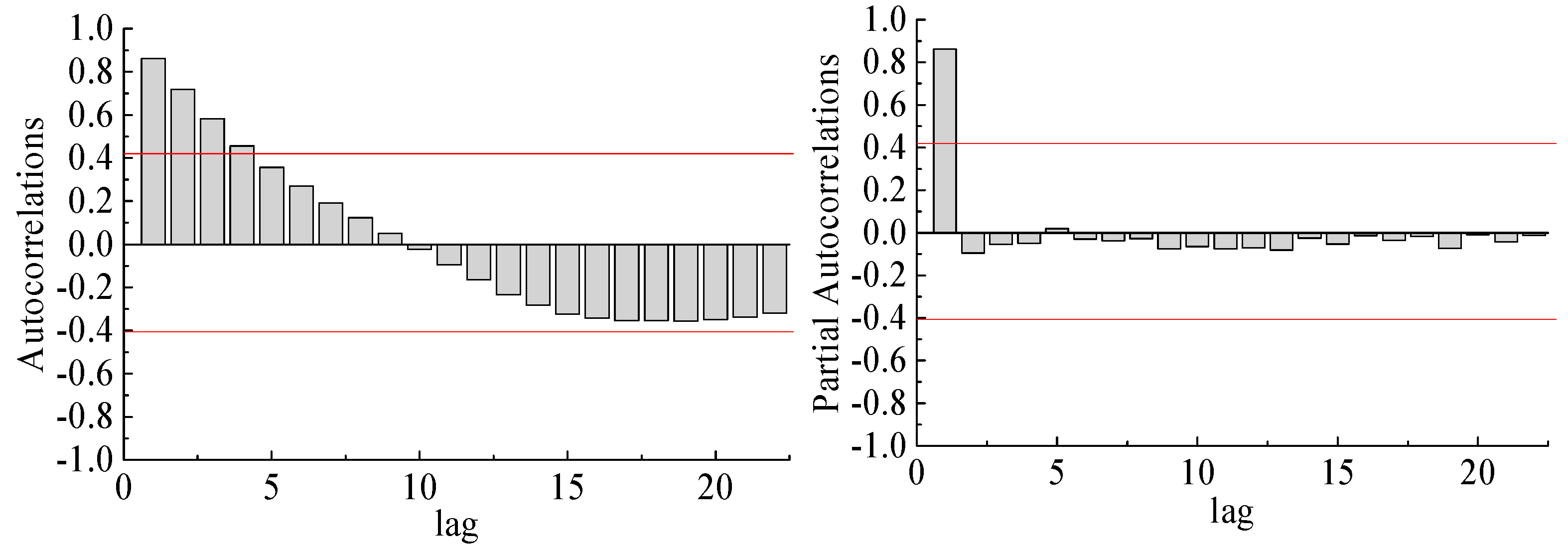
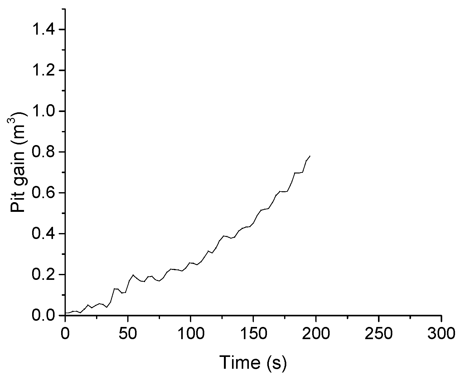
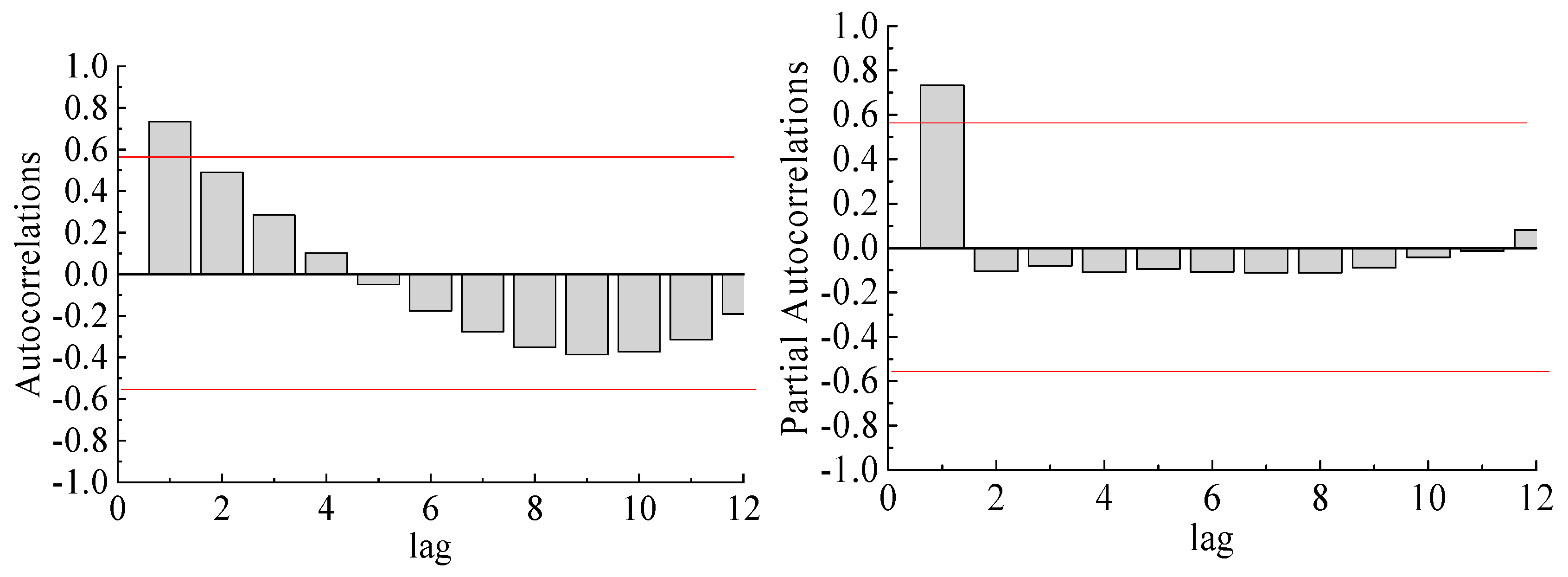
From Figure 2 it can be seen that there is a marked downward trend in the sequence diagram. Figure 3 shows the autocorrelation coefficient and the partial autocorrelation coefficient of the pit gain time series, and it can be seen that the autocorrelation coefficient decreases slowly to zero and the autocorrelation coefficient map shows obvious triangular symmetry. The unit root test results of the pit gain time series are shown in Table 1, and the probability (P) of the ADF test statistic is greater than 0.05. Therefore, the pit gain series is not a stationary sequence and can be derived from Figure 2, Figure 3, and Table 1. To establish the time series prediction model, differential processing is needed.
3.2. Processing of Non-Stationary Parameter Series
For non-stationary parameter series, it is necessary to process and extract the effective information in the sequence, that is, the deterministic information contained in the series. Generally, the difference method is used to extract the deterministic information of non-stationary series [28].
Figure 4 shows the autocorrelation coefficient and partial autocorrelation coefficient of the pit gain time series after the first-order difference. Table 2 shows the unit root test results of the pit gain time series after the first-order difference. As the probability (P) of the ADF test statistic is greater than 0.05, the series is still not a stationary sequence after the first-order difference, and second-order differential processing is needed.
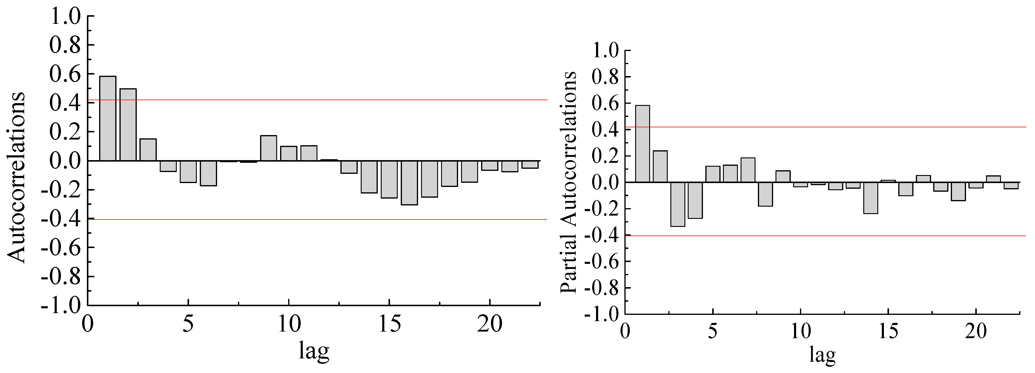
Figure 5 shows the autocorrelation coefficient and partial autocorrelation coefficient of the pit gain time series after the second-order difference; the second-order difference series has a strong short-term correlation. Table 3 shows the unit root test results of the pit gain time series after the second-order difference. The probability (P) of the ADF test statistic is less than 0.05. Therefore, the series is stable after the second-order difference, and the model can be established.
3.3. Model Identification and Order Determination
The values of the autocorrelation coefficient (ACF) and partial autocorrelation coefficient (PACF) are calculated to determine p and q, that is, to identify and order the model [29]:
where and .
According to the autocorrelation and partial autocorrelation diagram of the second-order difference of the pit gain series, shown in Figure 5, the preliminary order of the model can be determined. It can be seen from the figure that the autocorrelation coefficients fall within two standard deviations after delaying the first-order difference and exhibit tailing. The partial autocorrelation coefficients are within two standard deviations after delaying the first-order difference and exhibit tailing. Therefore, it can be preliminarily determined that p = 4 or 5 and q = 1, and the model can be preliminarily determined to be either ARIMA (4,2,1) or ARIMA (5,2,1).
3.4. Model Validity Test
After the model is fitted, it is necessary to test or evaluate the effectiveness of the fit of the model. If the fitting effect does not meet the evaluation requirements, it needs to be remodeled. This mainly includes a residual analysis and significant analysis of the parameters [30]:
3.4.1. Residual Analysis
For a model with a good degree of fit, the useful information in the measurement sequence should be extracted. The fitting residual term should have no information related to the sequence, that is, its residual term should tend toward a white noise sequence.
The white noise test process is as follows: it is assumed that the sequence values of the delay period, less than or equal to the m period, are independent of each other, and the Q-statistic method is used for analysis:
where n is the measurement sequence period and m is the delay period.
The Q-statistic approximately obeys the chi-square distribution with a degree of freedom of m:
It can be seen from Equation (7) that when the Q-statistic is greater than the quantile or if the P-statistic is greater than , then the hypothesis is accepted and the residual sequence is a white noise sequence.
3.4.2. Significance Test of Parameters
Through the significance test of the parameters, it can be tested whether the unknown parameter is significant to zero, which makes the fitted model more compact and more convenient for predictive calculation.
The test begins with the following assumptions:
where is the least-squares estimation.
obeys a normal distribution, i.e., , where .
Thus, a test statistic (T-test statistic) can be constructed for testing the significance of unknown parameters:
When , the parameters are significant. The probability (P-value) of the test statistics can also be used for analysis. When P is less than , the parameters are significant.
Table 4 shows the results of the model parameter significance statistic test (P-value), and models with P-values less than 0.05 are ARIMA (4,2,1)_d, ARIMA (4,2,1)_h, ARIMA (5,2,1)_l, and ARIMA (5,2,1)_p, that is, all the parameters of the these four models are significant.
3.5. Model Optimization
Since more than one model passes the test, to select the optimal model, the model needs to be optimized and selected. The criteria for optimal selection are the Akaike Information Criterion (AIC) and the Bayesian Information Criterion (SBC)—the optimal model being when the AIC and SBC of the fitted model are the smallest [31]:
where MLE is the maximum likelihood estimate and NUP is the number of unknown parameters in the model.
Table 5 shows the white noise test results and the AIC and SBC values of the four models’ residual sequences. It can be seen that the P-values of the Q-statistics of the ARIMA (4,2,1)_h and ARIMA (5,2,1)_p models are greater than 0.05, and their residual sequences are white noise sequences, which satisfy the white noise test. Compared with the AIC and SBC of the ARIMA (4,2,1)_h model and the ARIMA (5,2,1)_p model, the AIC (−3.9) and SBC (−3.7) of ARIMA (4,2,1)_h model are smaller, so the ARIMA (4,2,1)_h model is the best model.
3.6. Parameter Estimation
The parameter estimation determines the model structure and order to establish the ARIMA (p,d,q) and then estimate the value of the unknown parameter in the model. In this paper, the least-squares estimation is used for the parameter estimation [32].
For the ARIMA (p,d,q) model,
Its residual term is
The sum of the squared residuals is
The least-squares estimate of is a set of parameters that minimizes the sum of the squared residuals.
The model parameters are shown in Table 6.
3.7. Forecasting
Future parameters are predicted based on the principle of the minimum mean square error [33]. The ARIMA (p,d,q) model can be represented by a linear function of random perturbation terms, namely,
where are determined by .
satisfy the following formula:
Thus, the true value of can be obtained with
However, the parameters and cannot be directly obtained, so the estimated value of is
The mean square error between the true and estimated values is
In the case of minimizing the mean square error (when ), the estimated value of the l-period is
The l-period estimation error is
Therefore, the estimated value plus the estimated error is the true value of the prediction:
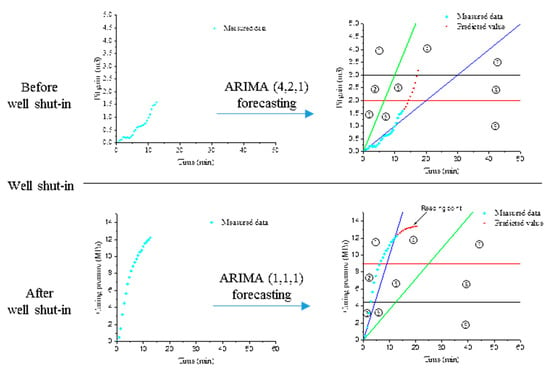
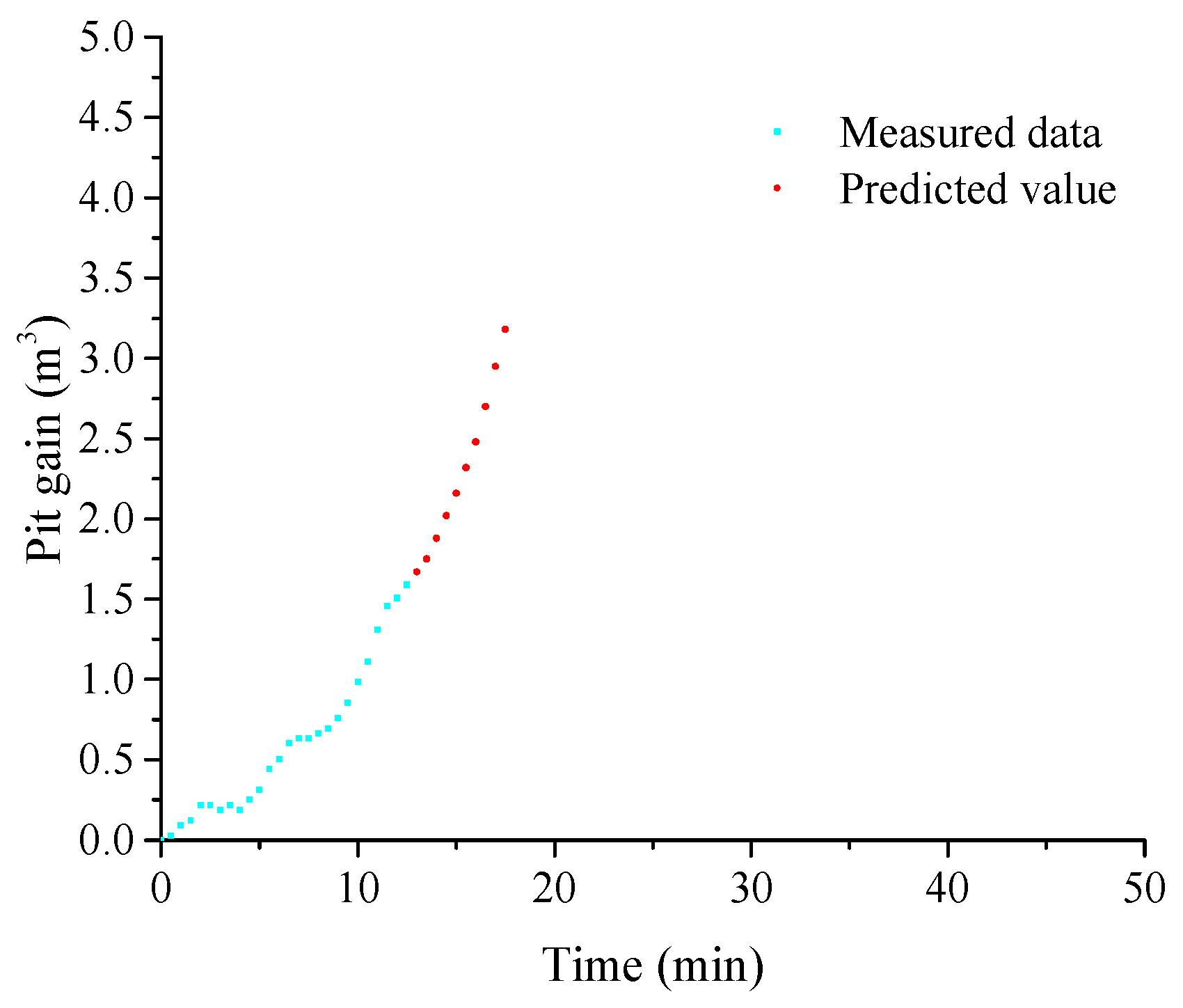
Figure 6 is the result of forecasting pit gain after 5 min using the ARIMA (4,2,1) model. It can be seen from the figure that the pit gain has not reached 2 m3 at 12 min, and the well has not been closed at this time. By predicting the pit gain after 5 min, the predicted pit gain has reached 3.18 m3 and it is also showing a gradually increasing trend.
3.8. Forecast Performance Measure
The mean relative error (MRE) is used for assessing the quality of the forecast. MRE can be considered as the mean of the relative values of the forecast errors and can be expressed with the following formula:
where is the realized value at time period t, is the forecast about that period, and N is the number of data points.
3.9. Kick Severity Analysis
3.9.1. Analysis of the Kick Severity before Closing the Well
It can be seen from the permeation fluid mechanics and natural gas reservoir engineering that when drilling a gas-bearing reservoir the negative pressure difference at the bottom of the well has not yet reached the boundary of the formation, so the fluid flow in the formation can be regarded as the plane radial flow in an infinitely homogeneous isotropic gas reservoir. At this point, the rate at which natural gas invades the wellbore is [34]
where is the gas flow rate from the formation into the wellbore in m3/d, is the supply pressure in MPa, is the bottom hole pressure in MPa, is the effective permeability in μm2, is the effective thickness of the gas reservoir layer in m, is the volume coefficient of gas, is the gas viscosity in mPa·s, is the natural gas compression factor, T is the formation temperature in K, is the pressure transmitting coefficient in μm2·MPa/(mPa·s), t is the invasion time in h, and is the borehole radius in m.
The amount of natural gas that invades the wellbore in t days is
where is the amount of natural gas that has invaded the wellbore in t time in m3 and t is the invasion time in h.
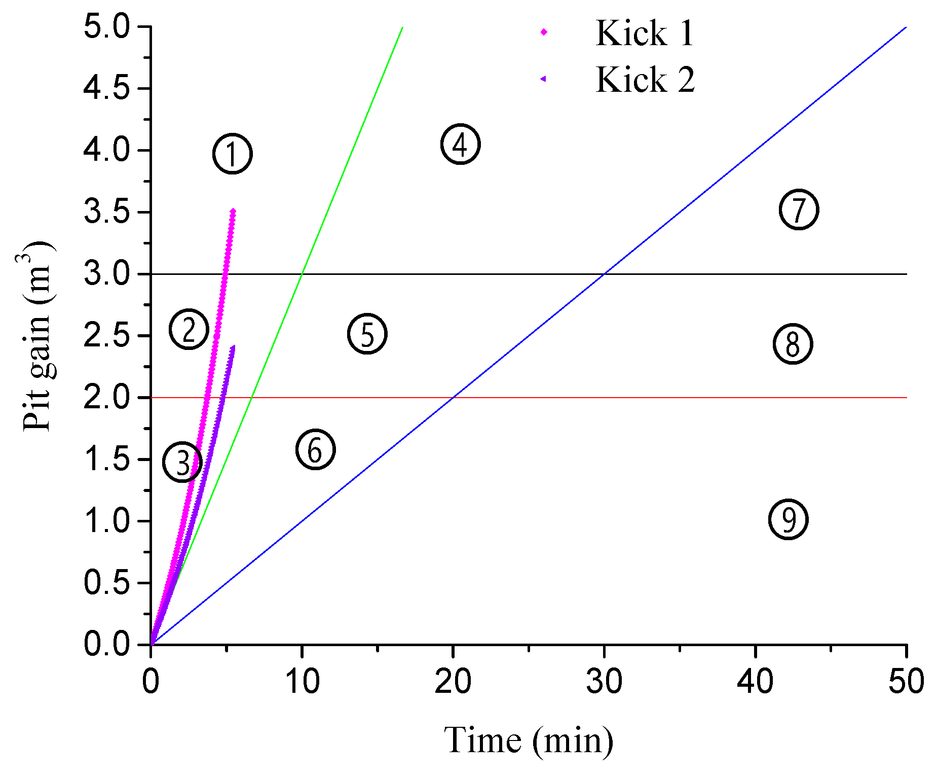
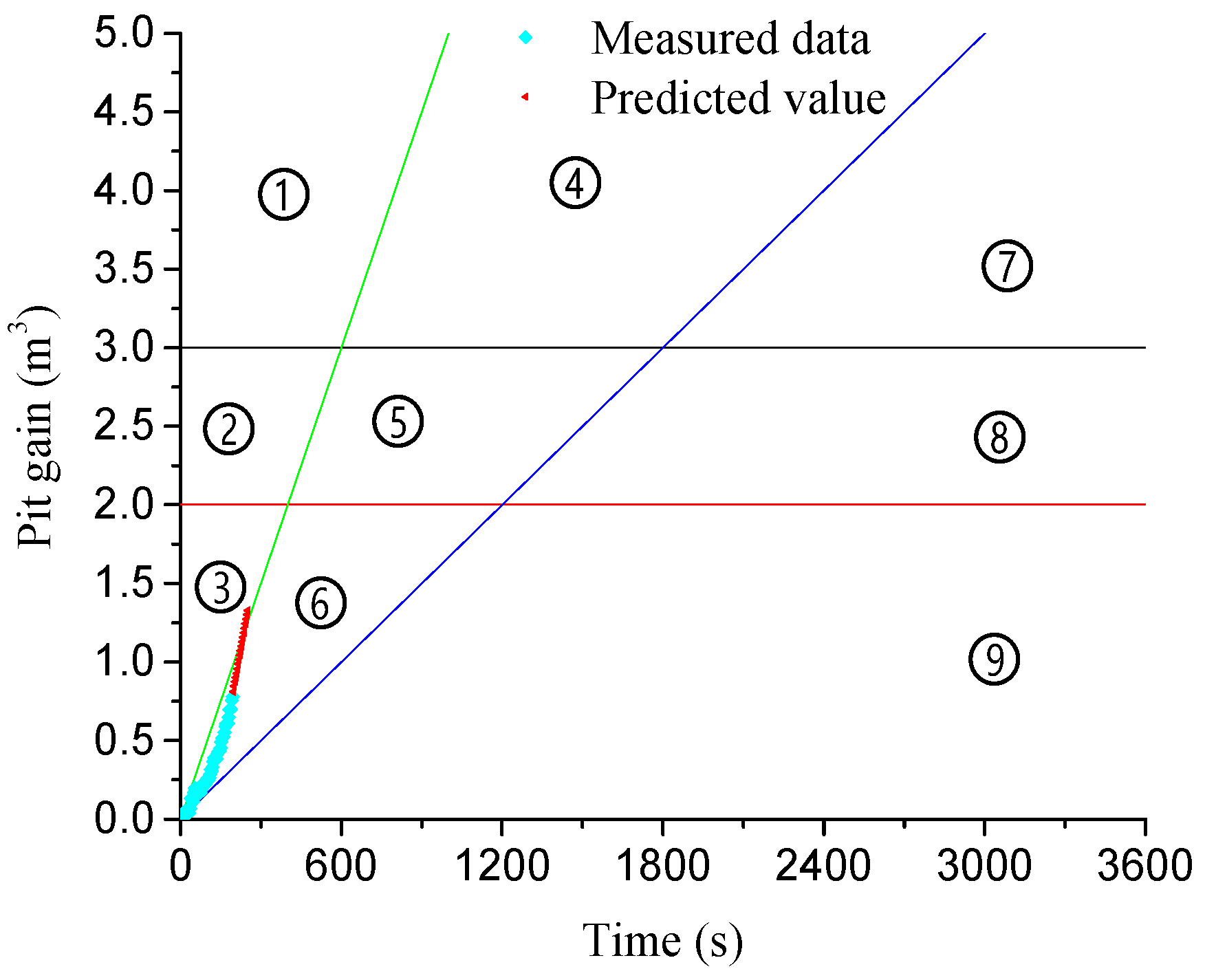
From Equation (27) and Equation (28), it can be seen that the amount of gas intrusion is related to the reservoir parameters, bottom hole pressure, and time. The pit gain and the growth rate of the pit gain (the change rate of pit gain with time) can reflect the severity of a kick. In the curve of pit gain over time, several horizontal lines are used to distinguish the pit gain level and several straight lines with different slopes are used to distinguish the pit gain rate. Therefore, the kick severity analysis chart before closing the well includes several horizontal lines of pit gain and several oblique lines of the pit gain change rate. According to the well control standard and related operation specifications of the Chuandong area in China [35], the maximum pit gain should not exceed 3 m3 when drilling the reservoir and the well should be shut in when the overflow is 2 m3. Moreover, according to relevant statistics in more than 100 wells, more than two-thirds of the wells had a time interval from the discovery of overflow to the blowout of less than 30 min with more than half of the two-thirds being within 10 min [36]. The kick severity analysis chart based on well control standards and statistical data before closing the well is shown in Figure 7.
Figure 7 is divided into nine regions according to the pit gain increment and the kick development time. Additionally, in Figure 7, there are pit gain vs. time curves for two kicks that are used to evaluate the kick severity. Kick 1 and Kick 2’s pit gains are located in Area ① and Area ②, respectively. Comparing the Kick 1 curve and the Kick 2 curve, the pit gain of Kick 1 is 3.5 m3, while Kick 2 has a pit gain of 2.5 m3 in the same time. The pit gain before the well closes is the direct parameter of the kick tolerance and is used to judge whether the well can be shut down safely and to select killing methods. The kick tolerance is a quantity that represents the amount of residual energy in the process of well killing after a kick occurs. The larger the pit gain’s volume, the smaller the kick tolerance, the greater the well shut-down risk, and the greater the risk of conventional killing. Thus, the kick severity of Area ① is greater than that of Area ②. The results are as follows: in Area ①, the pit gain is very large, with a rapid development trend and the greatest risk of kick; in Area ②, the pit gain is large, with a rapid development trend and a very high kick risk; in Area ③, the pit gain is less, but its development trend is rapid, and the kick risk is greater; in Area ④, the pit gain is very large, there is a certain development trend, and the kick risk is very high; in Area ⑤, the pit gain is large, there is a certain development trend, and the kick risk is relatively large; in Area ⑥, the pit gain is less, there is a slower development trend, and the kick risk is relatively small; in Area ⑦, the pit gain is very large, but the pit gain develops slowly, and there is a large kick risk; in Area ⑧, the pit gain is large, but the development is slow, and there is a certain kick risk; and in Area ⑨, the pit gain is small, the pit gain develops slowly, and the kick risk is small. The order of the kick severity before closing the well is ① > ② > ④ > ⑤ > ⑦ > ③ > ⑧ > ⑥ > ⑨.
3.9.2. Analysis of the Kick Severity after Shut-in
After well shut-in, the casing pressure will gradually increase under the influence of wellbore afterflow. When the bottom hole pressure and formation pressure are balanced, the casing pressure tends to be stable, and this point is the "analysis point" that is used to analyze the severity of the kick risk.
The increase in value of the casing pressure during shut-in depends on the difference between the formation pressure and the bottom hole pressure—the greater the difference, the greater the casing pressure, and the more serious the kick risk. Through the analysis of the casing pressure, the size of the unbalance between the bottom hole pressure and the formation pressure can be evaluated, and then the size of the kick risk can be analyzed.
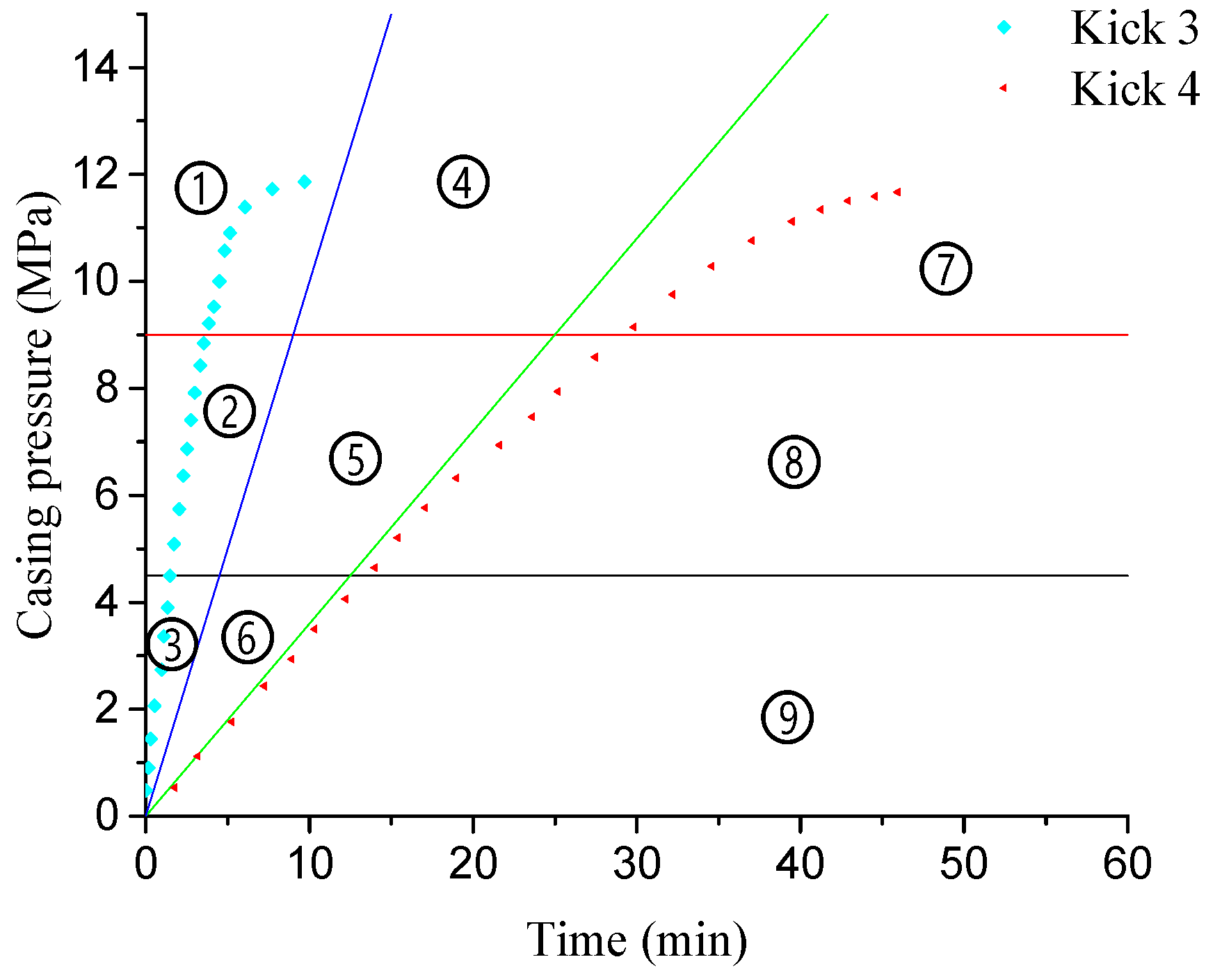
When the underbalanced pressure difference between the formation pressure and the bottom hole pressure is constant, the formation coefficient is proportional to the increase in the casing pressure, that is, the slope of the casing pressure and time can be used to characterize the formation coefficient. The larger the slope is, the larger the formation coefficient is, and the faster the casing pressure increases, the more serious the kick risk is [37]. Through the analysis of the casing pressure recovery curve, the size of the kick risk can be analyzed. The kick severity analysis chart based on the casing pressure recovery curve during the well shut-in period is shown in Figure 3.
In the shut-in casing pressure recovery curve, the pressure value of the analysis point represents the degree of unbalance between the formation pressure and the bottom hole pressure and several pressure value horizontal lines are used to distinguish the casing pressure level. The slope from the analysis point to the starting point indicates the speed at which the casing pressure recovers, which is affected by the formation coefficient. Therefore, the kick severity analysis chart during the well shut-in period includes several horizontal lines dividing the pressure level and several oblique lines dividing the rate of change in the casing pressure. According to information on some wells in the Sichuan Basin in China, the low-medium pressure limit is 4.5 MPa, the medium-high pressure limit is 9 MPa, the lower slope is tan20°, and the medium-high slope is tan45°, as shown in Figure 8. It should be noted that the specific values of the pressure limit and the curve slope in other regions were adjusted according to the different stratigraphic conditions of the corresponding regions [37].
Figure 8 is divided into nine regions according to the casing pressure and the casing pressure increase rate. Additionally, in Figure 8, there are casing pressure vs. time curves for two kicks that were used to evaluate the kick and well control severity. Kick 3 and Kick 4’s casing pressures are located in Area ① and Area ⑦, respectively. Comparing the Kick 3 curve and Kick 4 curve, it takes 10 min and 45 min to restore a stable casing pressure, respectively. Although the underbalanced pressure difference between the formation pressure and the bottom hole pressure is the same, the velocity of pressure transfer varied greatly. As the velocity of pressure transfer depends largely on the formation coefficient, such as permeability, porosity, and reservoir thickness, the larger the formation coefficient, the faster the pressure transfer velocity. During a well killing operation, by adjusting the opening of the ground valve, the bottom hole pressure should be controlled within a safe range above the formation pressure. However, in a high temperature and high pressure deep well, the complex law of bottom hole pressure changes making it difficult to maintain a safe range, which could cause a secondary kick and increases the difficulty of well killing. Owing to being under the same time and underbalanced pressure conditions, the larger the formation coefficient, the more gas is intruded, and the greater the well control risk. Thus, the kick and well control severity of Area ① is greater than that of Area ⑦. The results are as follows: in Area ①, the kick is very serious and the risk to well control is very large; in Area ②, the kick is serious and the well control risk is large; in Area ③, the kick severity is medium and the well control has a certain difficulty risk; in Area ④, the kick is more serious and the risk to well control is larger; in Area ⑤, the overflow is small and the well control has some risks; in Area ⑥, there is a slight risk of a kick and no well control; in Area ⑦, the kick is small and the well control has some risks; in Area ⑧, there is a slight risk of a kick and no well control; and in Area ⑨, there is no overflow risk and no well control risk. The order of the kick severity during the well closed period is ① > ② > ④ > ⑤ > ⑦ > ③ > ⑧ > ⑥ > ⑨.
4. Results and Discussion
In this section, the proposed method is applied to the kick severity forecast in several wells, which is based on the prediction of pit gain and casing pressure.
4.1. Analysis and Calculation of the Kick Severity before Closing the Well
4.1.1. Case Study One
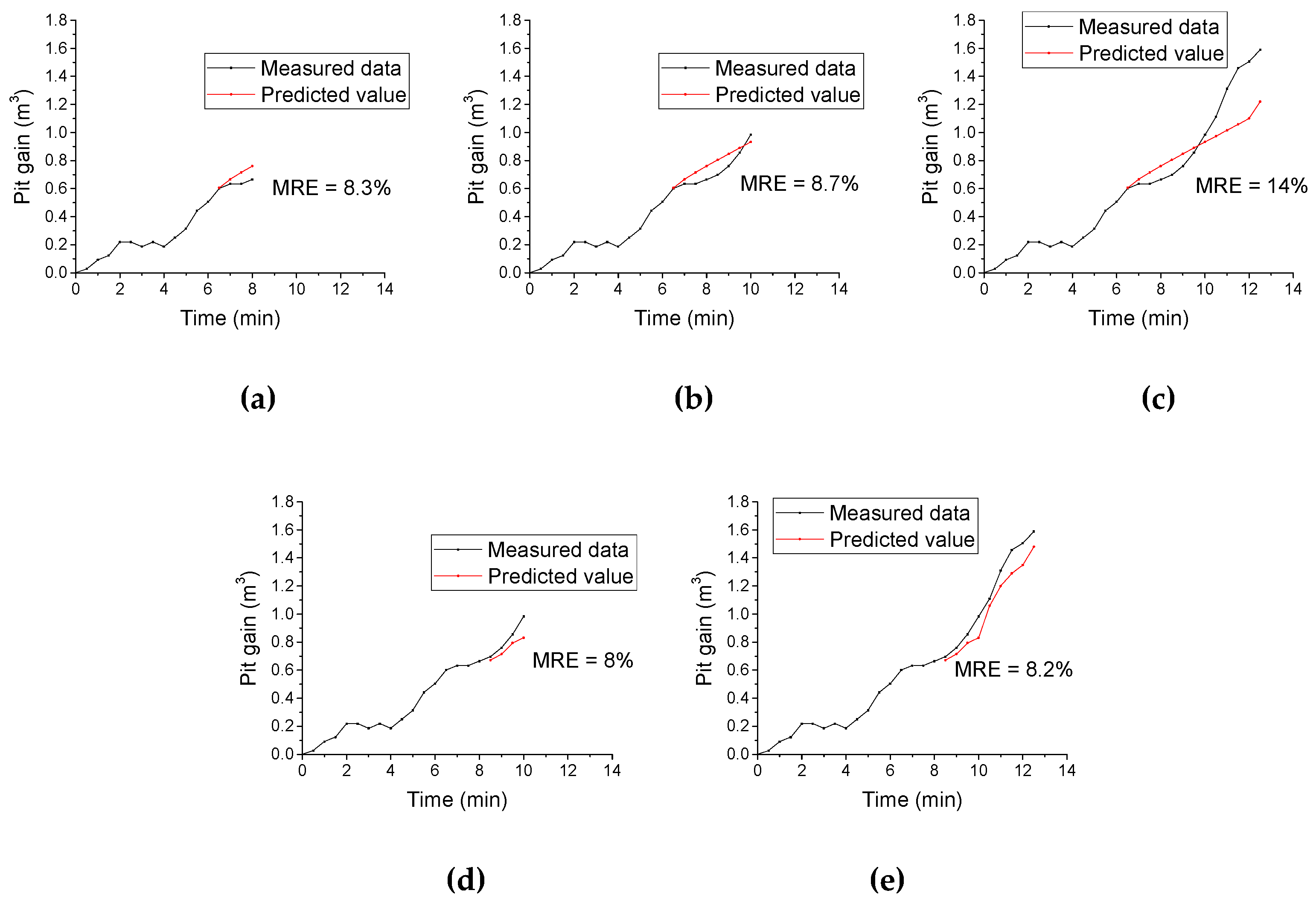
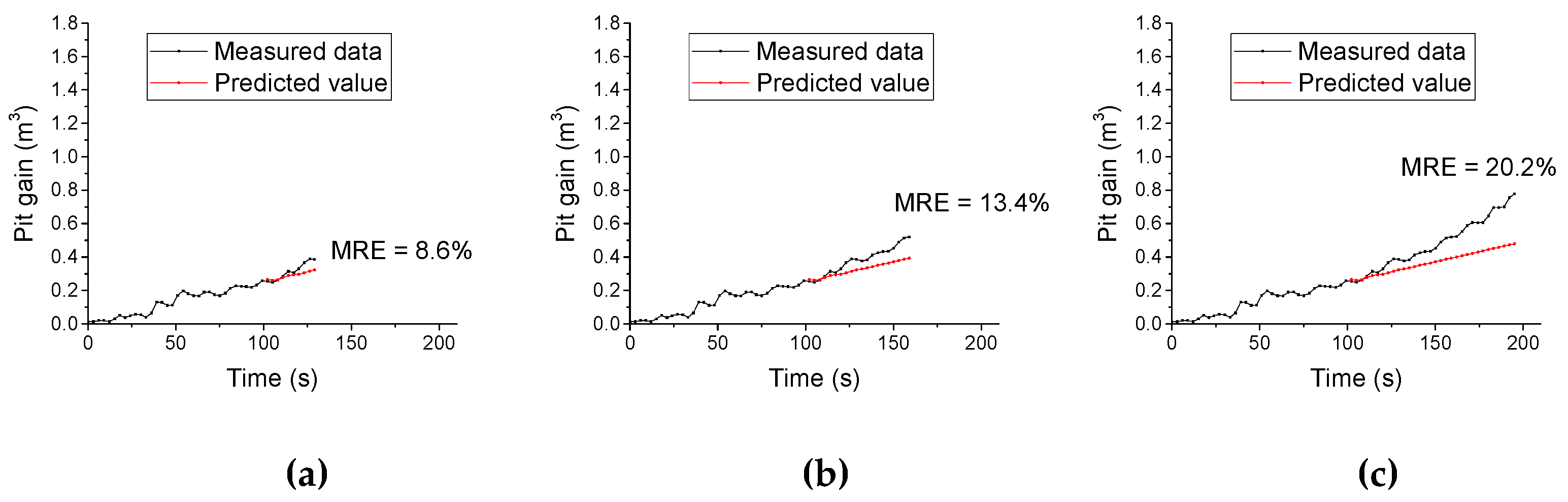
In Section 3, the pit gain forecasting model ARIMA (4,2,1) of well SC-X1 was established; Figure 9 shows the measured data and predicted values of pit gain vs. time in different periods.
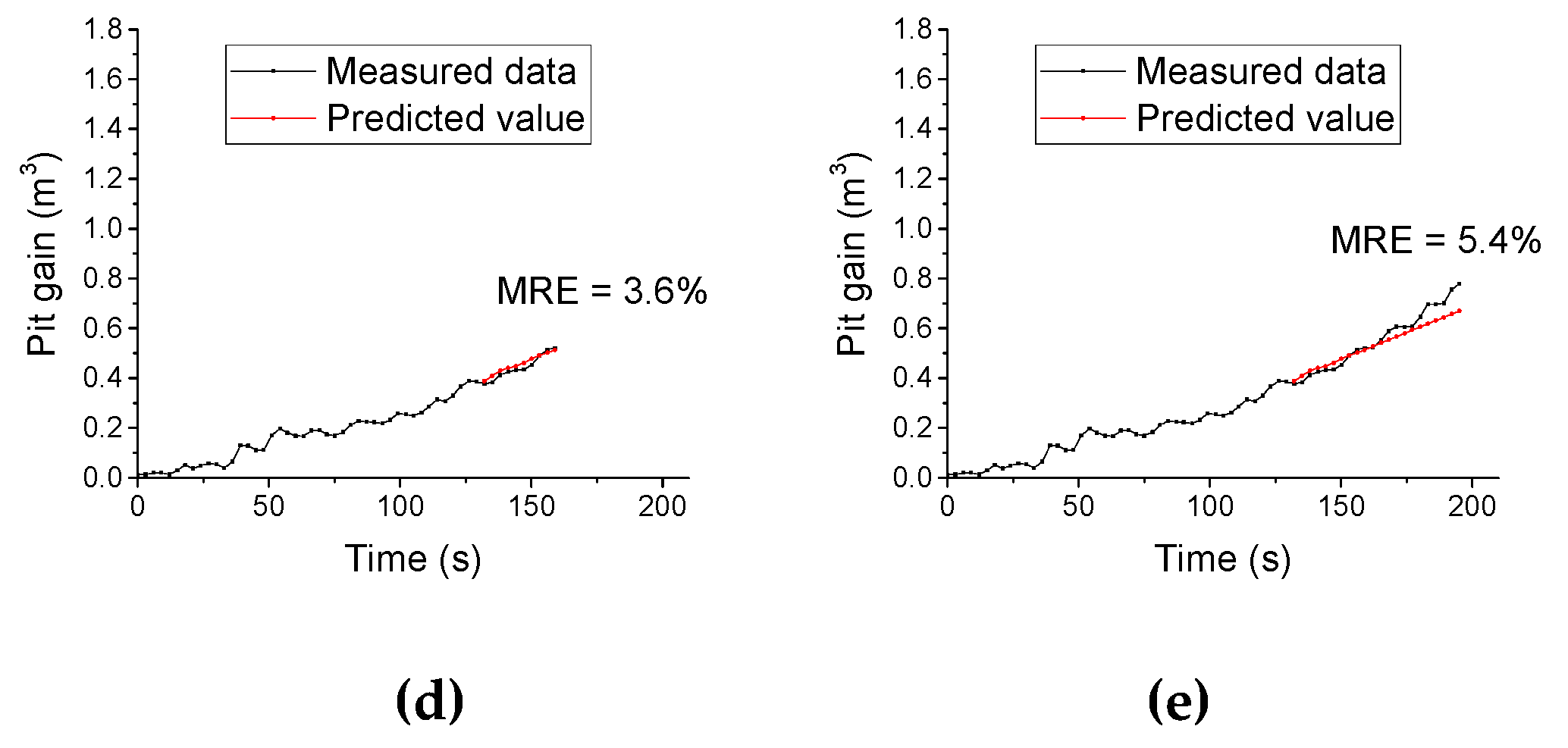
Figure 9a–c show that with an increase in prediction time, the MRE increases gradually (from 8.3% to 8.7% and then to 14%). Specifically, the prediction accuracy decreases with an increase in prediction time, which can also be obtained from Figure 9d,e. By comparing Figure 9a,d, we can see that the more measured data there are, the smaller the MRE is (8.3% and 8%), which can also be obtained from Figure 9b,e. Overall, the MRE based on the measurement data period of 0 to ~8.5 min is small (less than 8.2%).
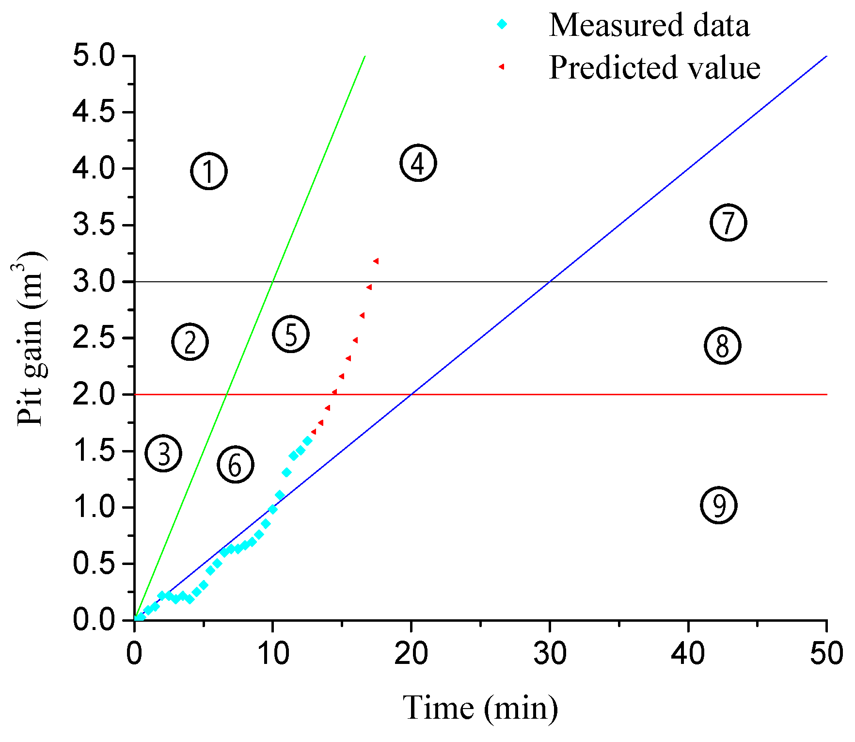
Figure 10 is the result of forecasting the pit gain after 5 min using the ARIMA (4,2,1) model. The forecasted curve is plotted in the kick severity analysis chart based on the pit gain volume increment. It can be seen from the figure that the data are located in Area ⑥ before the prediction, the pit gain has not reached 2 m3 at 12 min, and the well has not been closed at this time. By predicting the pit gain after 5 min, it can be seen that the pit gain curve is already in Area ④. At this time, the predicted pit gain has reached 3.18 m3 and is also showing a gradually increasing trend. The well control risk is already large—the well needs to be immediately shut down and the appropriate well control measures need to be selected.
4.1.2. Case Study Two
In this case, one well in [3] is used for analysis; the time sequence diagram of the pit gain before well shut-in is shown in Figure 11. Using the same modeling process as described in Section 3, the model ARIMA (2,2,1) is established. Figure 12 shows the measured data and predicted values of the pit gain vs. time in different periods.
From Figure 12, the same rule as Figure 9 can be obtained. Figure 12a–c show that with an increase in the prediction time, the MRE increases gradually (from 8.6% to 13.4% and then to 20.2%). Specifically, the prediction accuracy decreases with the increase in prediction time, which can also be obtained from Figure 12d,e. By comparing Figure 12a,d, it can be seen that the more measured data there are, the smaller the MRE is (8.6% and 3.6%), which can also be obtained from Figure 12b,e. Overall, the MRE based on the measurement data period 0 to ~129 s is small (less than 5.4%).
Figure 13 is the result of the forecasted pit gain in the next 54 s using the ARIMA (2,2,1) model. The forecasted curve is plotted in the kick severity analysis chart based on the pit gain volume increment. It can be seen from the figure that the data are located in Area ⑥ before the prediction, the pit gain is less, there is a slower development trend, and the kick risk is relatively small. By predicting the pit gain after 54 s, it can be seen that the pit gain curve is already in Area ③, and although the pit gain is less, its development trend is rapid and the kick risk is greater. Thus, it needs to be immediately shut down and the appropriate well control measures need to be selected.
4.2. Analysis and Calculation of the Kick Severity after Well Shut-In
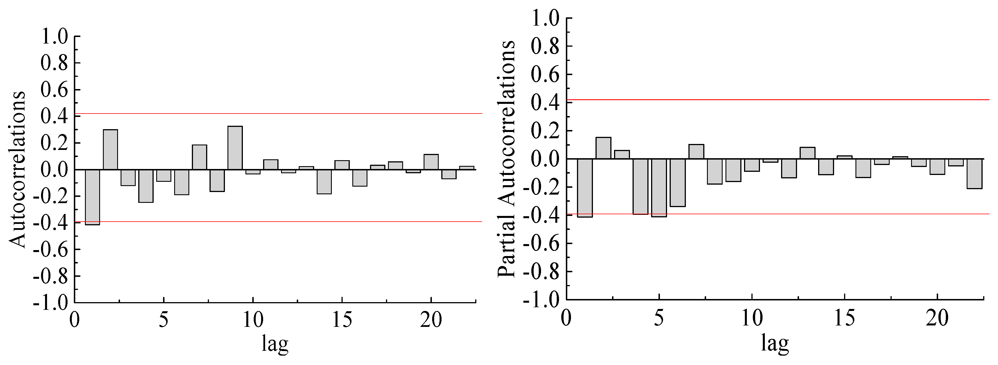
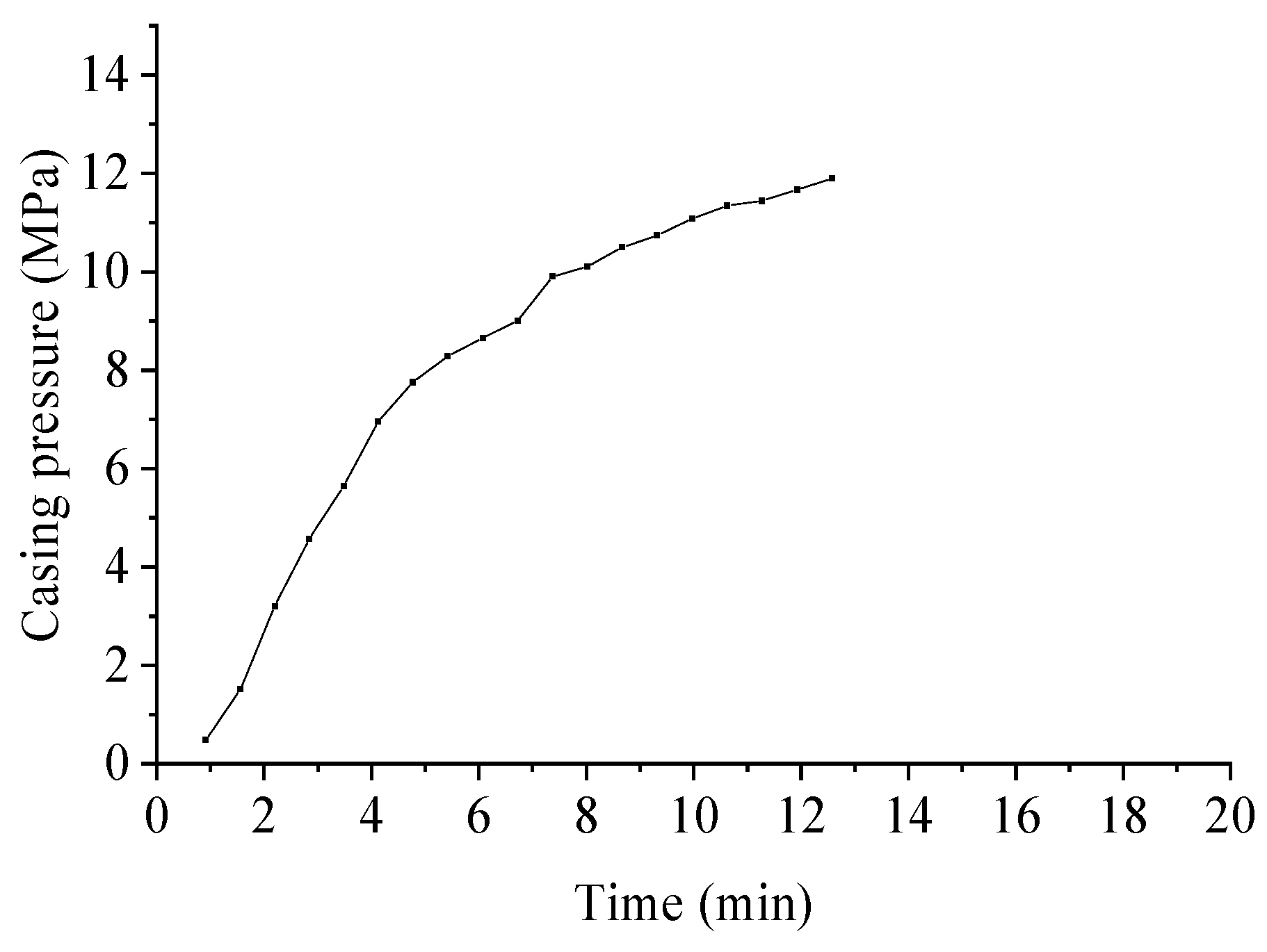
Figure 14 is the time sequence diagram of the casing pressure during well shut-in, and it can be seen that there is a marked upward trend in the sequence diagram. Figure 14 shows the autocorrelation coefficient and partial autocorrelation coefficient of the casing pressure time series. It shows that the autocorrelation coefficient decreases to zero slowly, and the autocorrelation coefficient graph shows obvious triangular symmetry. Therefore, the casing pressure sequence is not a stationary sequence and needs differential processing.
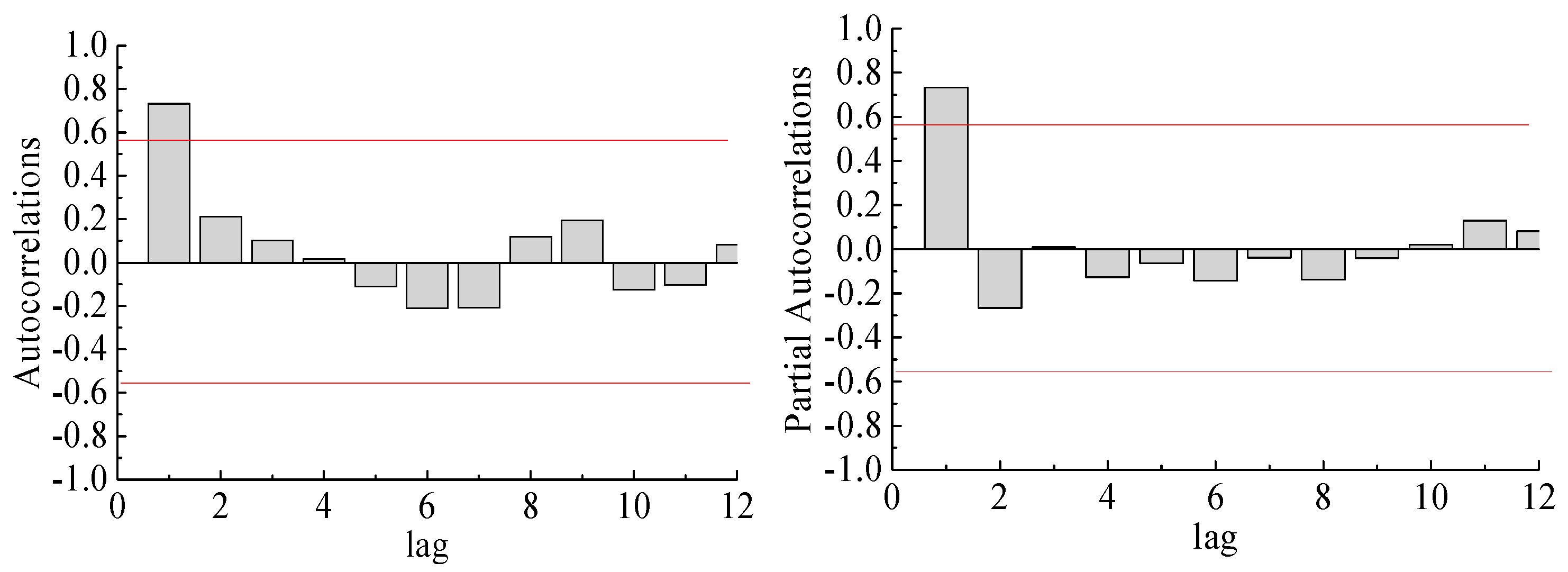
Figure 15 shows the autocorrelation coefficient and partial autocorrelation coefficient of the casing pressure time series after the first-order difference; the first-order difference series has a strong short-term correlation. Table 7 shows the unit root test results of the casing pressure time series after the first-order difference; the probability (P) of the ADF test statistic is less than 0.05. Therefore, the series after the first-order difference is stable, and the model can be established.
Based on the autocorrelation and partial autocorrelation diagram of the first-order difference of the casing pressure shown in Figure 16, the preliminary order of the model can be determined. It can be seen from the figure that both the autocorrelation coefficient and partial autocorrelation coefficient fall within two standard deviations after the delay of the first-order, and the model is established by ARIMA (1,1,1). Table 8 shows the residual white noise test of the ARIMA (1,1,1) model. The probability P-value of the Q-statistic is greater than 0.05, so the residual sequence is a white noise sequence, which satisfies the model’s requirements. Table 9 shows the ARIMA (1,1,1) model’s unknown parameter prediction and the statistic’s probability P-value. The P-value is less than 0.05, so the model meets the requirements.
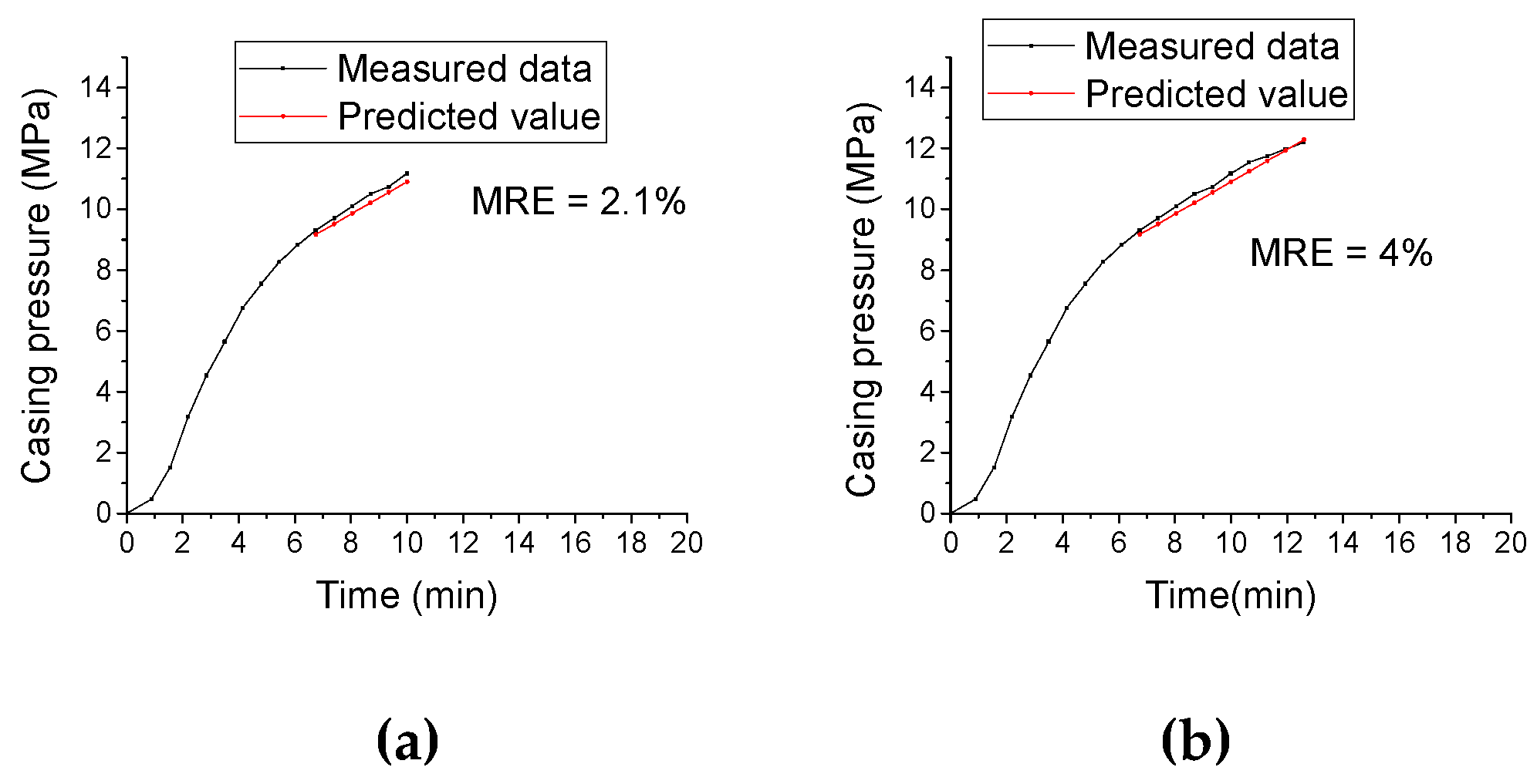
From Figure 17, the same rules as Figure 9 and Figure 12 can be obtained. Figure 17a,b show that with an increase in prediction time, the MRE increases gradually (from 2.1% to 4%). Specifically, the prediction accuracy decreases with the increase of prediction time. Generally speaking, the MRE is small (less than 4%).
Figure 18 shows the change in casing pressure after well shut-in. The ARIMA (1,1,1) model is constructed by the time series method to predict the future casing pressure. It is predicted that the reading point of the casing pressure will be in Area ④, the kick will be more serious, and the risk to well control will be larger, so it needs to be dealt with in time.
4.3. Discussion
The application of this paper can be divided into two stages—the prediction of pit gain before well shut-in and the prediction of casing pressure after well shut-in. After the occurrence of a kick, the prediction model is established based on the real-time data of the previous pit gain, the development trend of the pit gain is predicted, and the next step is taken with reference to the predicted pit gain. If the predicted pit gain is small (for example less than 2 m3), for the commonly used managed pressure drilling technology at present, the well may not need to be shut in. By adjusting the surface equipment of managed pressure drilling, the bottom hole pressure can be increased, the kick can be recycled out, and drilling time can be saved. If the predicted overflow is large (for example more than 2 m3), closing the well before 2 m3 can reduce formation fluid intrusion, which will be helpful to reduce the risk of a killing operation. After well shut-in, it is generally necessary to wait for casing pressure to return to a stable state on the drilling rig, then calculate the formation pressure, design a well killing construction report, and configure heavy mud. The prediction model in this paper can save killing time by predicting the casing pressure so that drilling operators can make preparations for killing the well in advance.
This method is suitable for short-term prediction but is not very good for long-term prediction. Our future work will consider the multimodel coupling method to improve long-term prediction accuracy.
5. Conclusions
Studies and field applications of measured data during drilling are kick warning and have been used to determine whether a kick occurs or not. However, there is no research on forecasting the severity of a kick by using measured data after a kick occurs.
In view of the time-varying characteristics of the characterization parameters after a kick, combined with the high degree of fitting a time series analysis method, the established time series model can be used for the prediction of pit gain and casing pressure.
Since pit gain and casing pressure can indirectly reflect the bottom hole condition, the changes in pit gain and casing pressure with time can be used to judge the severity of the kick. Combined with the prediction model, the severity of the kick can be predicted.
In this paper, the proposed method has been applied to pit gain forecasting in two wells and casing pressure forecasting in one well. The same rules can be seen in the case studies—an increase in prediction time, a gradual increase in MRE, and the more measured data, the smaller the MRE. Future work will consider the multimodel coupling method to improve long-term prediction accuracy.
The comparison between measured data and predicted data has shown that the proposed method has high prediction accuracy and repeatability. It has a certain guiding significance for the prediction of kick development trends, the analysis of kick severity, the selection of well control measures by engineers, and the reduction of the risk of a killing operation.
Author Contributions
Conceptualization, H.Y.; data curation, M.S.; formal analysis, M.S.; funding acquisition, Q.L.; investigation, M.S.; methodology, H.Y. and M.S.; project administration, H.Y. and Q.L.; resources, Q.L.; software, M.S. and J.Z.; supervision, H.Y., Q.L., and L.D.; validation, M.S.; visualization, M.S.; writing—original draft, M.S.; writing—review and editing, H.Y.
Funding
The authors greatly appreciate the support provided by the China National Science and Technology Major Project (2016ZX05020-006) and the China Scholarship Council (File No. 201708515156).
Acknowledgments
The authors are also grateful for the support provided by the University of Regina.
Conflicts of Interest
The authors declare no conflict of interest.
References
- Vajargah, A.K. Pressure Signature of Gas Influx. Ph.D. Thesis, University of Tulsa, Tulsa, OK, USA, 2013. [Google Scholar]
- Weishaupt, M.A.; Omsberg, N.P.; Jardine, S.I.; Patterson, D.A. Rig Computer System Improves Safety for Deep HP/HT Wells by Kick Detection and Well Control Monitoring; Society of Petroleum Engineers: Richardson, TX, USA, 1991. [Google Scholar] [CrossRef]
- Sun, X.; Sun, B.; Zhang, S.; Wang, Z.; Gao, Y.; Li, H. A new pattern recognition model for gas kick diagnosis in deepwater drilling. J. Pet. Sci. Eng. 2018, 167, 418–425. [Google Scholar] [CrossRef]
- Andia, P.; Israel, R.R. A Cyber-Physical Approach to Early Kick Detection; Society of Petroleum Engineers: Richardson, TX, USA, 2018. [Google Scholar] [CrossRef]
- Shi, X.; Zhou, Y.; Zhao, Q.; Jiang, H.; Zhao, L.; Liu, Y.; Yang, G. A new method to detect influx and loss during drilling based on machine learning. In Proceedings of the International Petroleum Technology Conference, Beijing, China, 26–28 March 2019. [Google Scholar] [CrossRef]
- Alouhali, R.; Aljubran, M.; Gharbi, S.; Al-yami, A. Drilling Through Data: Automated Kick Detection Using Data Mining; Society of Petroleum Engineers: Richardson, TX, USA, 2018. [Google Scholar] [CrossRef]
- Hargreaves, D.; Jardine, S.; Jeffryes, B. Early Kick Detection for Deepwater Drilling: New Probabilistic Methods Applied in the Field; Society of Petroleum Engineers: Richardson, TX, USA, 2001. [Google Scholar] [CrossRef]
- Pournazari, P.; Ashok, P.; van Oort, E.; Unrau, S.; Lai, S. Enhanced Kick Detection with Low-Cost Rig Sensors Through Automated Pattern Recognition and Real-Time Sensor Calibration; Society of Petroleum Engineers: Richardson, TX, USA, 2015. [Google Scholar] [CrossRef]
- Unrau, S.; Torrione, P.; Hibbard, M.; Smith, R.; Olesen, L.; Watson, J. Machine Learning Algorithms Applied to Detection of Well Control Events; Society of Petroleum Engineers: Richardson, TX, USA, 2017. [Google Scholar] [CrossRef]
- Brakel, J.; Tarr, B.; Cox, W.; Jorgensen, F.; Straume, H.V. SMART Kick Detection: First Step on the Well-Control Automation Journey; Society of Petroleum Engineers: Richardson, TX, USA, 2015. [Google Scholar] [CrossRef]
- Billingham, J.; Thompson, M.; White, D.B. Advanced Influx Analysis Gives More Information Following a Kick; Society of Petroleum Engineers: Richardson, TX, USA, 1993. [Google Scholar] [CrossRef]
- Avelar, C.S.; Ribeiro, P.R.; Sepehrnoori, K. Deepwater gas kick simulation. J. Pet. Sci. Eng. 2009, 67, 13–22. [Google Scholar] [CrossRef]
- Gao, Y.H.; Sun, B.J.; Zhao, X.X.; Wang, Z.Y. Dynamic simulation of kicks in deepwater drilling. J. Chin. Univ. Petrol. 2010, 6, 66–70. [Google Scholar]
- Sun, B.J.; Wang, Z.Y.; Gong, P.B.; Song, R. Application of a seven-components multiphase flow model to deepwater well control. Acta Pet. Sin. 2011, 32, 1042–1049. [Google Scholar]
- Ren, M.; Li, X.; Wang, Y.; Yin, B. Judgement method of kick rate and height based on standpipe and casing pressure. Oil Drill. Prod. Technol. Shiyou Zuancai Gongyi 2012, 34, 16–19. [Google Scholar]
- Aarsnes, U.J.F.; Ambrus, A.; Di Meglio, F.; Vajargah, A.K.; Aamo, O.M.; van Oort, E. A simplified two-phase flow model using a quasi-equilibrium momentum balance. Int. J. Multiph. Flow 2016, 83, 77–85. [Google Scholar] [CrossRef]
- Meng, Y.; Xu, C.; Wei, N.; Li, G.; Li, H.; Duan, M. Numerical simulation and experiment of the annular pressure variation caused by gas kick/injection in wells. J. Nat. Gas Sci. Eng. 2015, 22, 646–655. [Google Scholar] [CrossRef]
- Meipeng, R.E.N.; Xiangfang, L.I.; Shujie, L.I.U. Characteristics of wellbore pressure change during shut-in after blowout. J. China Univ. Pet. 2015, 39, 113–119. [Google Scholar]
- Sen, P.; Roy, M.; Pal, P. Application of ARIMA for forecasting energy consumption and GHG emission: A case study of an Indian pig iron manufacturing organization. Energy 2016, 116, 1031–1038. [Google Scholar] [CrossRef]
- Ruby-Figueroa, R.; Saavedra, J.; Bahamonde, N.; Cassano, A. Permeate flux prediction in the ultrafiltration of fruit juices by ARIMA models. J. Membr. Sci. 2017, 524, 108–116. [Google Scholar] [CrossRef]
- Biu, V.T.; Ikiensikimama, S.S. Understanding Crude Oil Price Variation Using Time Series Analysis; Society of Petroleum Engineers: Richardson, TX, USA, 2012. [Google Scholar] [CrossRef]
- Zhao, C.; Wang, B.; GUO, P. The risk probability prediction of drilling operation site using ARIMA model. Xinjiang Pet. Geol. 2013, 4. [Google Scholar]
- Gupta, S.; Fuehrer, F.; Jeyachandra, B.C. Production Forecasting in Unconventional Resources Using Data Mining and Time Series Analysis; Society of Petroleum Engineers: Richardson, TX, USA, 2014. [Google Scholar] [CrossRef]
- Olominu, O.; Sulaimon, A.A. Application of Time Series Analysis to Predict Reservoir Production Performance; Society of Petroleum Engineers: Richardson, TX, USA, 2014. [Google Scholar] [CrossRef]
- Chatfield, C. The Analysis of Time Series; Chapman and Hall/CRC: New York, NY, USA, 2016. [Google Scholar]
- Brockwell, P.J.; Davis, R.A.; Calder, M.V. Introduction to Time Series and Forecasting; Springer: New York, NY, USA, 2002; Volume 2. [Google Scholar]
- Gu, L. Time Series Analysis Prediction and Control; China Statistics Press: Beijing, China, 1997. [Google Scholar]
- Wang, Y. Application of Time Series Analysis; Renmin University Press: Beijing, China, 2005. [Google Scholar]
- Shumway, R.H.; Stoffer, D.S. Time Series Analysis and its Applications: With R Examples; Springer: New York, NY, USA, 2017. [Google Scholar]
- Touati, B. Integration of Seasonal ARIMA in the GR4J Conceptual Model for Runoff Forecasting of Lijiang Catchment. Ph.D. Thesis, Guangxi University, Nanning, China, 2018. [Google Scholar]
- Agiakloglou, C.; Newbold, P. Empirical evidence on Dickey-Fuller-type tests. J. Time Ser. Anal. 1992, 13, 471–483. [Google Scholar] [CrossRef]
- Agyemang, B. Autoregressive Integrated Moving Average (ARIMA) Intervention Analysis Model for the Major Crimes in Ghana. (The case of the Eastern Region). Ph.D. Thesis, Kwame Nkrumah University of Science and Technology, Kumasi, Ghana, 2012. [Google Scholar]
- Box, G.E.; Jenkins, G.M.; Reinsel, G.C.; Ljung, G.M. Time Series Analysis: Forecasting and Control; John Wiley & Sons: New York, NY, USA.
- Li, X. Underground Oil Gas Seepage Mechanics; Petroleum Industry Press: Beijing, China, 2005. [Google Scholar]
- Chen, A. 12.23 Small Blowout Cause Serious Disaster: Anniversary Ceremony of 12.23 Great Blowout Accident of Chuandong Drilling Company; Technical Report No. 02:34-38; PetroChina Southwest Oil and Gasfield Company: Chengdu, China, 2005. [Google Scholar]
- Changxiu, C.; Shitian, Z.E.N.G. Several technical problems considered emphatically for drilling natural gas wells. Nat. Gas Ind. 2002, 22, 54–55. [Google Scholar]
- Xu, H.; LI, X. A determination method of the level of well control difficulty before well kicking. Nat. Gas Ind. 2009, 5, 27. [Google Scholar]
Figure 1.
Steps to establish the forecast model, AC is the autocorrelation coefficient and PAC is the partial autocorrelation coefficient.
Figure 1.
Steps to establish the forecast model, AC is the autocorrelation coefficient and PAC is the partial autocorrelation coefficient.

Figure 2.
Time sequence diagram of pit gain.

Figure 3.
Autocorrelation coefficient and partial autocorrelation coefficient of the pit gain time series.
Figure 3.
Autocorrelation coefficient and partial autocorrelation coefficient of the pit gain time series.

Figure 4.
Autocorrelation coefficient and partial autocorrelation coefficient of pit gain time series after the first-order difference.
Figure 4.
Autocorrelation coefficient and partial autocorrelation coefficient of pit gain time series after the first-order difference.

Figure 5.
Autocorrelation coefficient and partial autocorrelation coefficient of the pit gain time series after the second-order difference.
Figure 5.
Autocorrelation coefficient and partial autocorrelation coefficient of the pit gain time series after the second-order difference.

Figure 6.
Measured data and predicted values of pit gain vs. time.

Figure 7.
Kick severity analysis chart before well shut-in.

Figure 8.
Kick severity analysis chart during the well shut-in period.

Figure 9.
Measured data and predicted values of pit gain vs. time in different periods: (a) prediction period 6.5–8 min, (b) prediction period 6.5–10 min, (c) prediction period 6.5–12.5 min, (d) prediction period 8.5–10 min, and (e) prediction period 8.5–12.5 min.
Figure 9.
Measured data and predicted values of pit gain vs. time in different periods: (a) prediction period 6.5–8 min, (b) prediction period 6.5–10 min, (c) prediction period 6.5–12.5 min, (d) prediction period 8.5–10 min, and (e) prediction period 8.5–12.5 min.

Figure 10.
Kick severity analysis result using forecasted pit gain.

Figure 11.
Time sequence diagram of pit gain.

Figure 12.
Measured data and predicted values of the pit gain vs. time in different periods: (a) prediction period 99–129 s, (b) prediction period 99–159 s, (c) prediction period 99–195 s, (d) prediction period 129–159 s, and (e) prediction period 129–195 s.
Figure 12.
Measured data and predicted values of the pit gain vs. time in different periods: (a) prediction period 99–129 s, (b) prediction period 99–159 s, (c) prediction period 99–195 s, (d) prediction period 129–159 s, and (e) prediction period 129–195 s.


Figure 13.
Kick severity analysis result using the forecasted pit gain.

Figure 14.
Time sequence diagram of the casing pressure during well shut-in.

Figure 15.
Autocorrelation coefficient and partial autocorrelation coefficient of casing pressure time series.
Figure 15.
Autocorrelation coefficient and partial autocorrelation coefficient of casing pressure time series.

Figure 16.
Autocorrelation coefficient and partial autocorrelation coefficient of the casing pressure time series after the first-order difference.
Figure 16.
Autocorrelation coefficient and partial autocorrelation coefficient of the casing pressure time series after the first-order difference.

Figure 17.
Measured data and predicted value of casing pressure vs. time in different periods: (a) prediction period 6.75–10 min and (b) prediction period 6.75–12.6 min.
Figure 17.
Measured data and predicted value of casing pressure vs. time in different periods: (a) prediction period 6.75–10 min and (b) prediction period 6.75–12.6 min.

Figure 18.
Results of the kick severity analysis using the predicted casing pressure.


Table 1.
Unit root test results of the pit gain time series.
| Statistics | Probability P | ||
|---|---|---|---|
| Test Statistics of ADF | 3.49 | 1 | |
| Critical value of the test | 1% Level | −3.81 | - - |
| 5% Level | −3.02 | - - | |
| 10% Level | −2.65 | - - | |
ADF is the augmented Dickey–Fuller.
Table 2.
Unit root test results of the pit gain time series after the first-order difference.
| Statistics | Probability P | ||
|---|---|---|---|
| Test Statistics of ADF | −2.32 | 0.17 | |
| Critical value of the test | 1% Level | −3.78 | - - |
| 5% Level | −3.01 | - - | |
| 10% Level | −2.64 | - - | |
Table 3.
Unit root test results of the pit gain time series after the second-order difference.
| Statistics | Probability P | ||
|---|---|---|---|
| Test statistics of ADF | −4.54 | 0.0025 | |
| Critical value of the test | 1% Level | −3.86 | - - |
| 5% Level | −3.04 | - - | |
| 10% Level | −2.66 | - - | |
Table 4.
Results of the model parameter significance statistic test (P-value).
| Model | C | AR(1) | AR(2) | AR(3) | AR(4) | AR(5) | MA(1) | |
|---|---|---|---|---|---|---|---|---|
| ARIMA (4,2,1) | a | 0.0001 | 0.4269 | 0.0954 | 0.1898 | 0.0092 | 0 | |
| b | 0.2333 | 0.1009 | 0.7544 | 0.0031 | 0.001 | |||
| c | 0.0372 | 0.921 | 0.0073 | 0.001 | ||||
| d | 0.0151 | 0.0044 | 0.0003 | |||||
| e | 0.0001 | 0.1524 | 0.2888 | 0.0282 | 0.0001 | |||
| f | 0.0004 | 0.2145 | 0.0062 | 0 | ||||
| g | 0.0004 | 0.6243 | 0.1266 | 0.0027 | 0 | |||
| h | 0.0001 | 0.049 | 0.0009 | 0 | ||||
| ARIMA (5,2,1) | a | 0.0001 | 0.8719 | 0.0311 | 0.5338 | 0.0106 | 0.2114 | 0 |
| b | 0 | 0.0372 | 0.479 | 0.0067 | 0.1029 | 0 | ||
| c | 0.1186 | 0 | 0.6073 | 0.0724 | 0.2626 | 0.0068 | ||
| d | 0 | 0.6756 | 0.0325 | 0.004 | 0.0833 | 0 | ||
| e | 0.6893 | 0.0486 | 0.4462 | 0.3219 | 0.8929 | 0.0002 | ||
| f | 0.6508 | 0.0482 | 0.7756 | 0.2628 | 0.0002 | |||
| g | 0 | 0.8892 | 0.0401 | 0.0279 | 0.0003 | |||
| h | 0.343 | 0 | 0.0958 | 0.2713 | 0 | |||
| i | 0.4383 | 0 | 0.1029 | 0.945 | 0.0072 | |||
| j | 0.0007 | 0.2377 | 0.2332 | 0.055 | 0.0009 | |||
| k | 0 | 0.0854 | 0.0035 | 0.0447 | 0 | |||
| l | 0 | 0.0331 | 0.0224 | 0 | ||||
| m | 0.0001 | 0.6014 | 0.0166 | 0.0001 | ||||
| n | 0.0013 | 0.4441 | 0.0072 | 0.0003 | ||||
| o | 0.5813 | 0 | 0.1888 | 0 | ||||
| p | 0 | 0.0033 | 0 | |||||
Table 5.
White noise test results and Akaike Information Criterion (AIC) and Bayesian Information Criterion (SBC) values of the residual sequences.
Table 5.
White noise test results and Akaike Information Criterion (AIC) and Bayesian Information Criterion (SBC) values of the residual sequences.
| Model | AIC | SBC | Delay Order | Q-Statistics | P-Value | Whether to Pass the Test |
|---|---|---|---|---|---|---|
| ARIMA (4,2,1)_d | −4.69 | −4.55 | 6 | 16.11 | 0.003 | No |
| 12 | 21.42 | 0.018 | ||||
| ARIMA (4,2,1)_h | −3.9 | −3.7 | 6 | 7.91 | 0.05 | Yes |
| 12 | 13.04 | 0.16 | ||||
| ARIMA (5,2,1)_l | −4 | −3.81 | 6 | 10.01 | 0.018 | No |
| 12 | 16.85 | 0.051 | ||||
| ARIMA (5,2,1)_p | −3.7 | −3.6 | 6 | 6.68 | 0.15 | Yes |
| 12 | 10.91 | 0.36 |
Table 6.
Model parameters of ARIMA (4,2,1)_h.
| Variable | C | AR(2) | AR(4) | MA(1) |
|---|---|---|---|---|
| Coefficient | 0.0005 | 0.348 | −0.684 | −0.954 |
Table 7.
Unit root test results of the casing pressure time series after the first-order difference.
Table 7.
Unit root test results of the casing pressure time series after the first-order difference.
| Statistics | Probability P | ||
|---|---|---|---|
| Test statistics of ADF | −5.5 | 0.0019 | |
| Critical value of the test | 1% Level | −4.3 | - - |
| 5% Level | −3.2 | - - | |
| 10% Level | −2.75 | - - | |
Table 8.
White noise test results and AIC and SBC values of the residual sequences.
| Model | AIC | SBC | Delay Order | Q-Statistics | P-Value | Whether to Pass the Test |
|---|---|---|---|---|---|---|
| ARIMA (1,1,1) | −3.26 | −3.15 | 6 | 2.82 | 0.59 | Yes |
Table 9.
Model parameters of ARIMA (1,1,1).
| Variable | C | AR(1) | MA(1) |
|---|---|---|---|
| Coefficient | 0.19 | 0.76 | −0.99 |
| Probability | 0.006 | 0 | 0 |
© 2019 by the authors. Licensee MDPI, Basel, Switzerland. This article is an open access article distributed under the terms and conditions of the Creative Commons Attribution (CC BY) license (http://creativecommons.org/licenses/by/4.0/).
Share and Cite
MDPI and ACS Style
Yin, H.; Si, M.; Li, Q.; Zhang, J.; Dai, L. Kick Risk Forecasting and Evaluating During Drilling Based on Autoregressive Integrated Moving Average Model. Energies 2019, 12, 3540. https://0-doi-org.brum.beds.ac.uk/10.3390/en12183540
AMA Style
Yin H, Si M, Li Q, Zhang J, Dai L. Kick Risk Forecasting and Evaluating During Drilling Based on Autoregressive Integrated Moving Average Model. Energies. 2019; 12(18):3540. https://0-doi-org.brum.beds.ac.uk/10.3390/en12183540
Chicago/Turabian StyleYin, Hu, Menghan Si, Qian Li, Jinke Zhang, and Liming Dai. 2019. "Kick Risk Forecasting and Evaluating During Drilling Based on Autoregressive Integrated Moving Average Model" Energies 12, no. 18: 3540. https://0-doi-org.brum.beds.ac.uk/10.3390/en12183540
Note that from the first issue of 2016, this journal uses article numbers instead of page numbers. See further details here.