1. Introduction
As of 2009, the expansion of wind power in the Brazilian electrical energy mix [
1,
2] was bolstered by a bidding mechanism that promoted competitiveness among different energy sources. This auction-based systematic concept favored the reduction of electricity prices, making wind power generation competitive with other well-explored power sources within the Brazilian electric power sector, such as hydro and thermal [
3,
4]. Furthermore, it was shown that it would be preferable, at competitive prices, to meet the Brazilian new demand for energy with only renewable sources such as wind instead of thermal power [
5].
Due to the stochastic nature of wind resources (i.e., a characteristic that determines variability in its availability), predicting wind power generation is an uncertain process and, thereby, acquiring knowledge of the historical behavior of wind is essential to estimate how much electricity a wind farm can produce and deliver to the grid [
6,
7,
8]. Wind resources vary in different temporal scales, from the shortest (seconds), to intermediate (hours to days), to longer timescales (months to years to decades) [
9]. It can be worrisome if interannual variability is neglected when designing a wind farm, to the extent that it could lead to overconfidence in the wind resources [
10,
11]. Several authors address the interannual variability as an issue to be dealt with if a better balance between electricity production and demand is sought [
10,
11,
12,
13,
14,
15]. Countries like Brazil, which lack the access to wind data recorded over a broad area and over long, multi-decadal periods, face the task of estimating its wind power potential where only short-term datasets resulting from recent wind measurement campaigns are available, since these are not able to represent the wind interannual variability. For that challenge to be overcome, the use of reanalysis data and measure-correlate-predict (MCP) methods is necessary.
MCP is a technique that is able to hindcast wind resources in a given target location where periodical measurements of wind speed and direction are carried out over a short period of time (usually from 12 to 36 months) [
7]. The methodology is an important step of the wind resource assessment (WRA), which can historically characterize the local wind behavior. However, wind data that is representative for longer timescales is required for the MCP and WRA to provide accurate knowledge about the local long-term wind variability and also to estimate the power output of a wind farm throughout its multidecadal lifespan [
7,
16]. Even though presenting significant uncertainties, reanalysis databases are commonly used to fill the gap in locations lacking long-term reference datasets because they result from a combination of different meteorological observations and numerical weather prediction models, providing coverage for large areas and long periods [
17,
18]. The MCP, as much as other WRA steps and reanalysis databases themselves, is subject to an uncertainty degree inherent to the unpredictability of the wind behavior. Thereby, the identification and quantification of this group of uncertainties is relevant when it comes to reliably determining the local wind energy potential [
19], which in turn directly affects the financial structure of wind power projects [
20,
21].
In Brazil, there is a minimum duration regarding the wind measurement campaign for a project to be able to participate in energy auctions. This minimum length for short-term datasets was extended from 24 to 36 whole months from 2017 onwards [
22]. The duration of the campaign is a relevant matter, since it indirectly dictates the volume of data to be used in the MCP, determining the concurrent period of data between target and reference locations. Longer periods of measurement tend to better outline the local wind variability [
16,
23]. Therefore, this recent Brazilian measure could improve the understanding of wind resources natural variability and, consequently, lead to a probable reduction regarding the group of uncertainties that pervades the WRA. Moreover, it is expected that new wind farm projects could more accurately reflect the reality of wind power generation in Brazil.
Few authors have studied the length of the concurrent data between short and long-term datasets. In [
16], Rogers et al. stated that the longer the short-term dataset, the smaller the standard deviation of MCP predictions of mean wind speed becomes. Also, in [
23], Taylor et al. affirmed that by increasing the duration of data collection it is possible to reduce the uncertainty in wind speed. Yet no research proposed to evaluate if longer short-term datasets could improve the WRA by influencing its overall uncertainty and, ultimately, the wind power output estimation. Given the aforementioned, the contribution of this article regards the assessment of how the uncertainty related to the long-term historical characterization of wind resources in a target location is affected by the increase in the wind measurement campaign timespan. Subsequently, the research aims to analyze if this longer monitoring period could promote enhancements in the estimation of power generation in a hypothetical scenario of a wind farm set in that target location.
3. Results and Discussion
In each of the six combinations between time series belonging to the target location (and its following measurement heights) and time series from the reference location, the tendency to reduce the historical uncertainty regarding the increase in the length of the wind monitoring campaign was evident. In relation to the 2 year duration, all the cases showed an average reduction of 18%, 29%, 35%, and 40% when, respectively, one, two, three, and four years were added to the monitoring campaign, as observed in
Table 5.
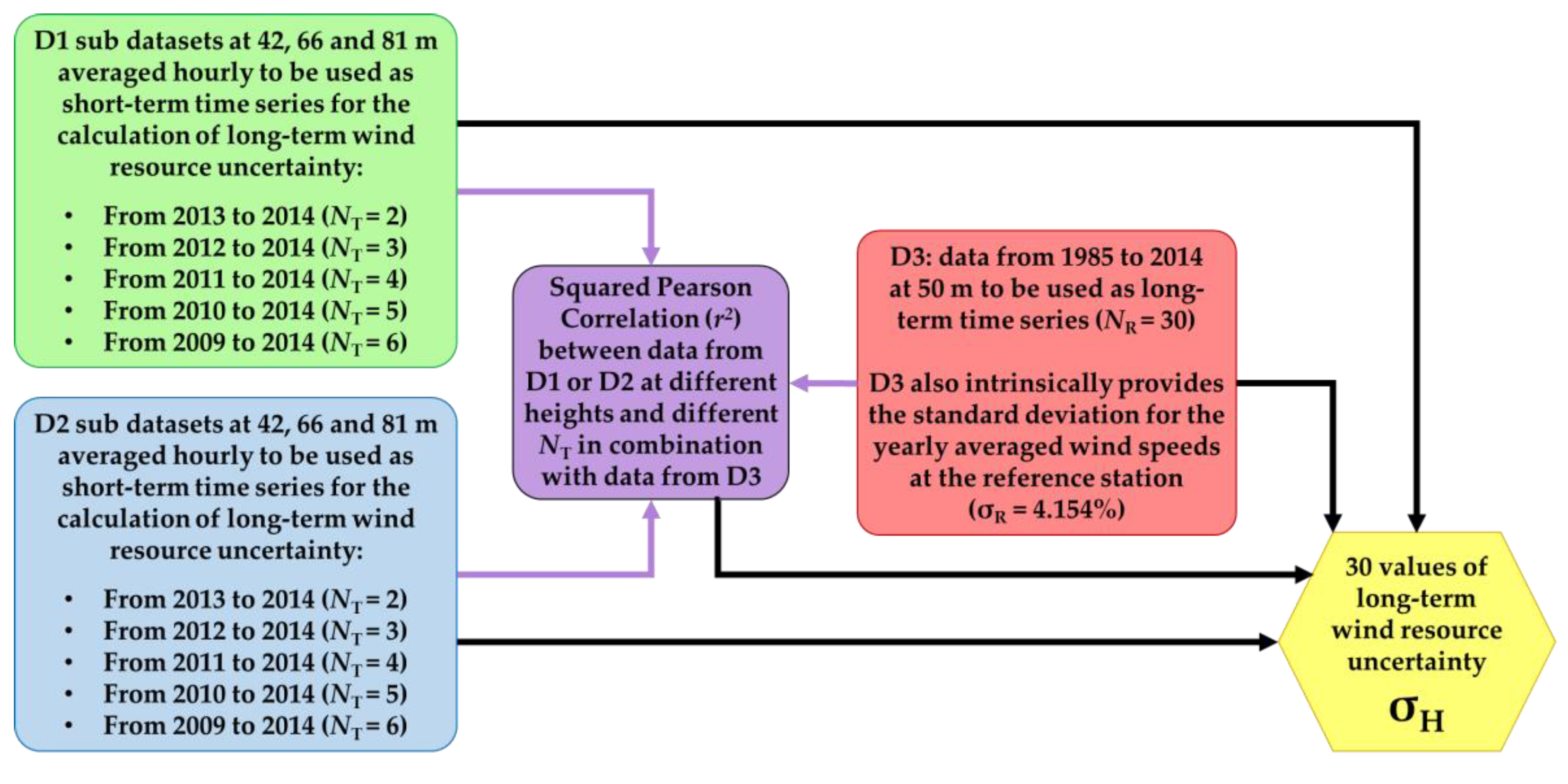
The long-term wind resource uncertainty is included in the
OU as a single type of uncertainty among all of those presented in
Table 4. When aggregated in Equation (5), all these uncertainty types result in the
OU. The calculation of
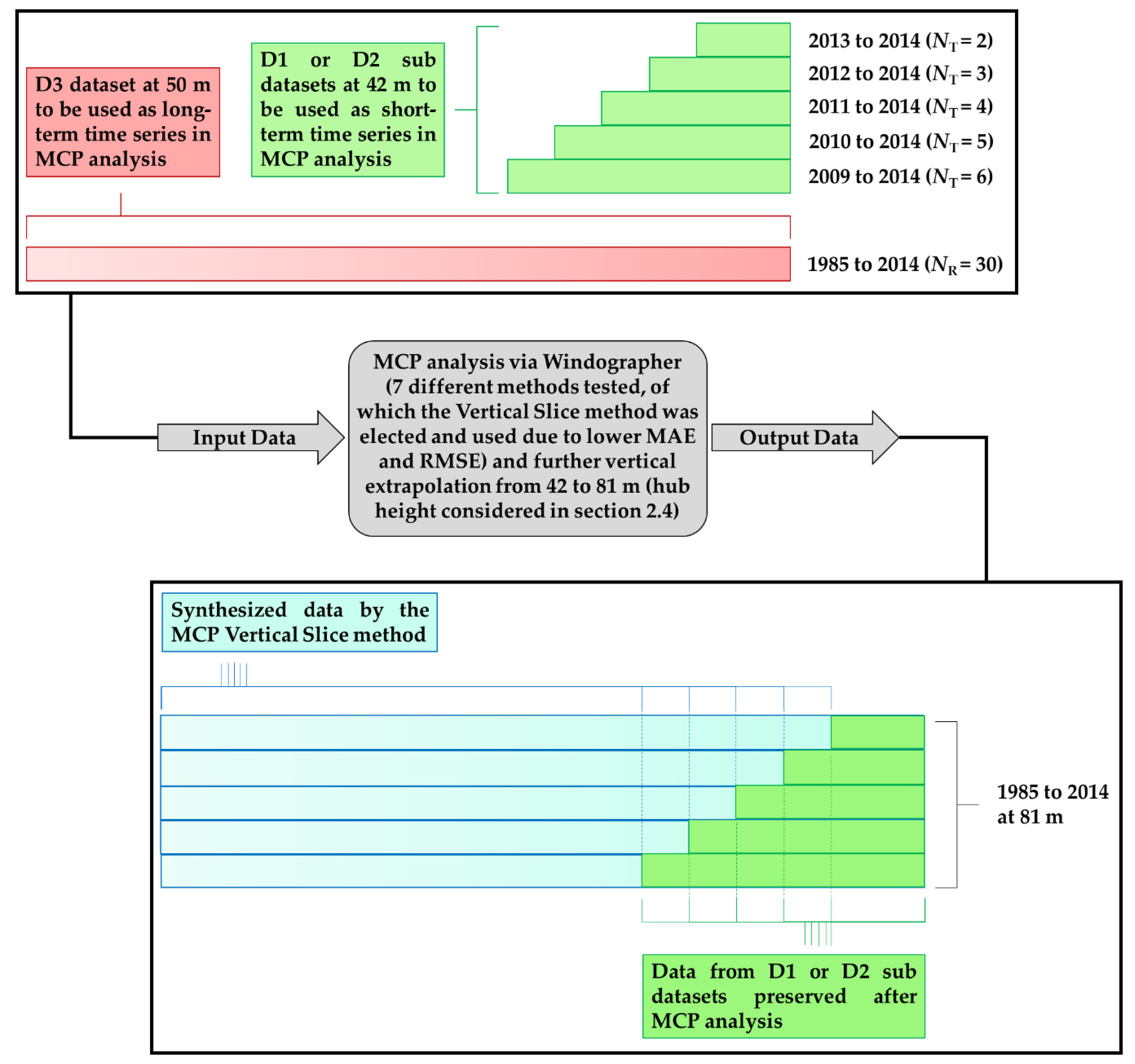
OU is associated to the resulting long-term time series synthesized by the MCP Vertical Slice method and took into consideration sub datasets from D1 or D2 (both only at 42 m, since these sub datasets were the ones inputted in the MCP analysis) as well as D3. In that sense, the different values of this historical characterization uncertainty were subject to different wind monitoring campaigns durations and, in combination with the fixed values considered for the other uncertainty types, resulted in different values for
OU, as verified in
Table 6.
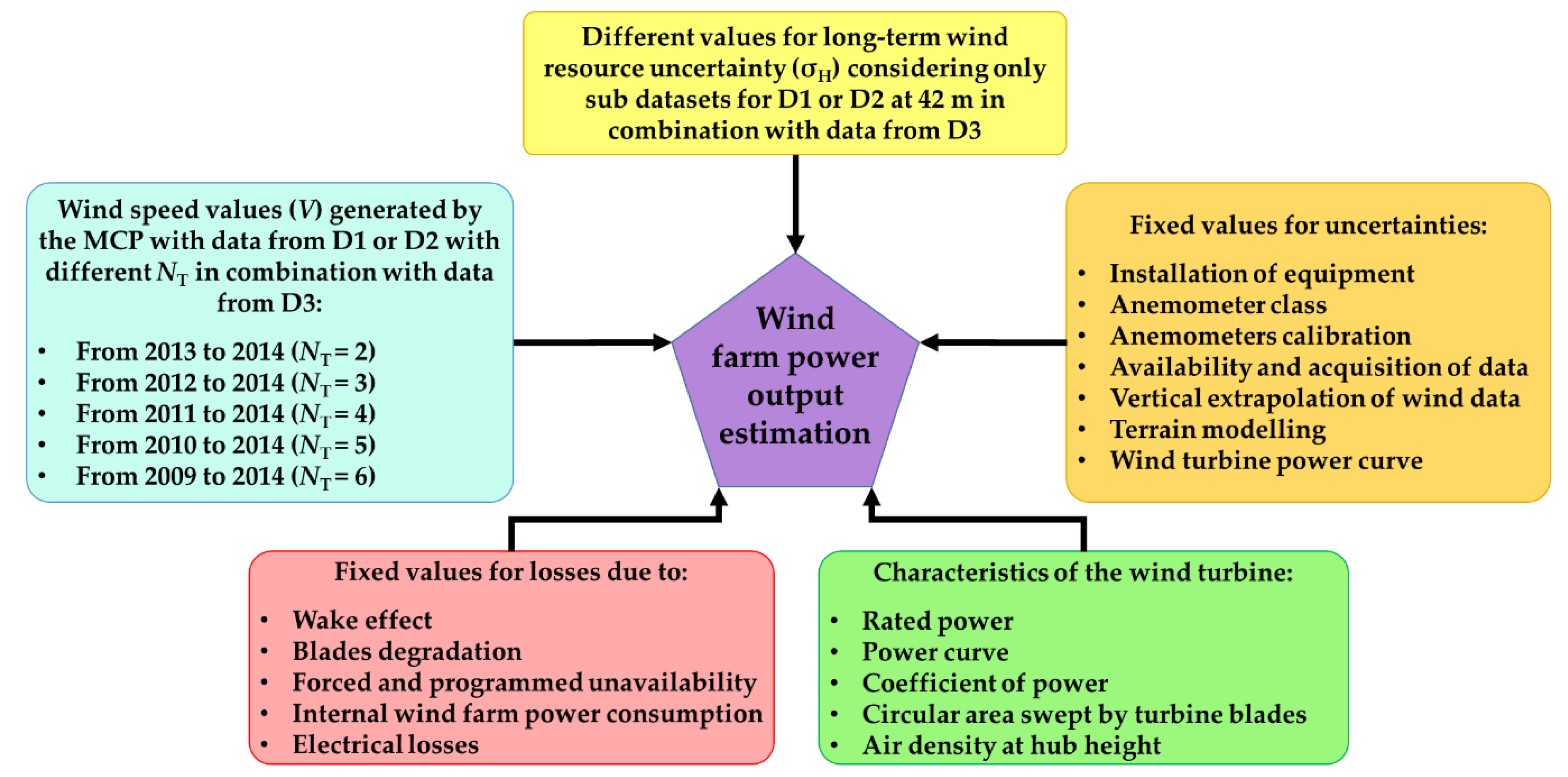
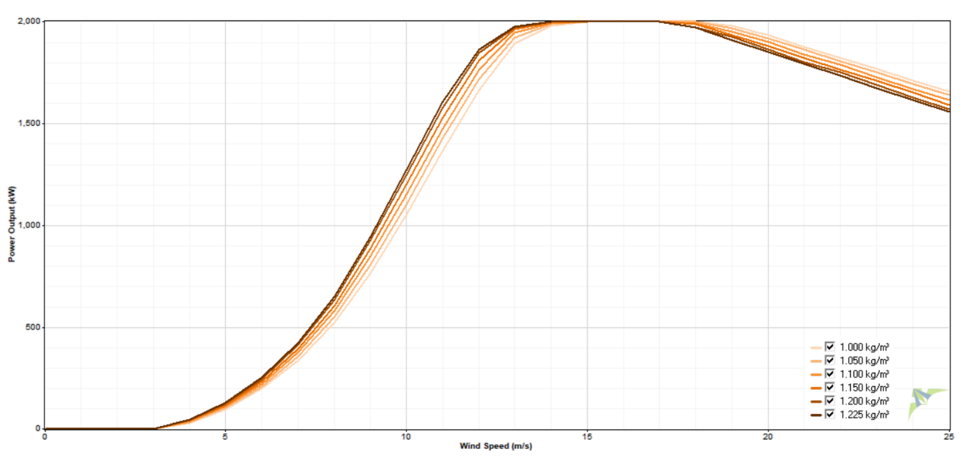
The MCP-synthesized time series were then used to estimate the wind power production considering a hypothetic wind farm of 15 wind turbines. The estimation was made by a tool from the Windographer software that automatically executes Equation (6). Arbitrarily, a 2 MW rated power wind turbine with a hub at 80 m above ground level was elected (Alstom ECO 80/2000 Class II), which is approximately the same height of the MCP extrapolated resulting synthetic data. Its power curve according to air density is seen in
Figure 5 [
65]. Hence, a wind farm with 15 of these turbines would account for an installed capacity of 30 MW. The results are shown in
Table 7 and
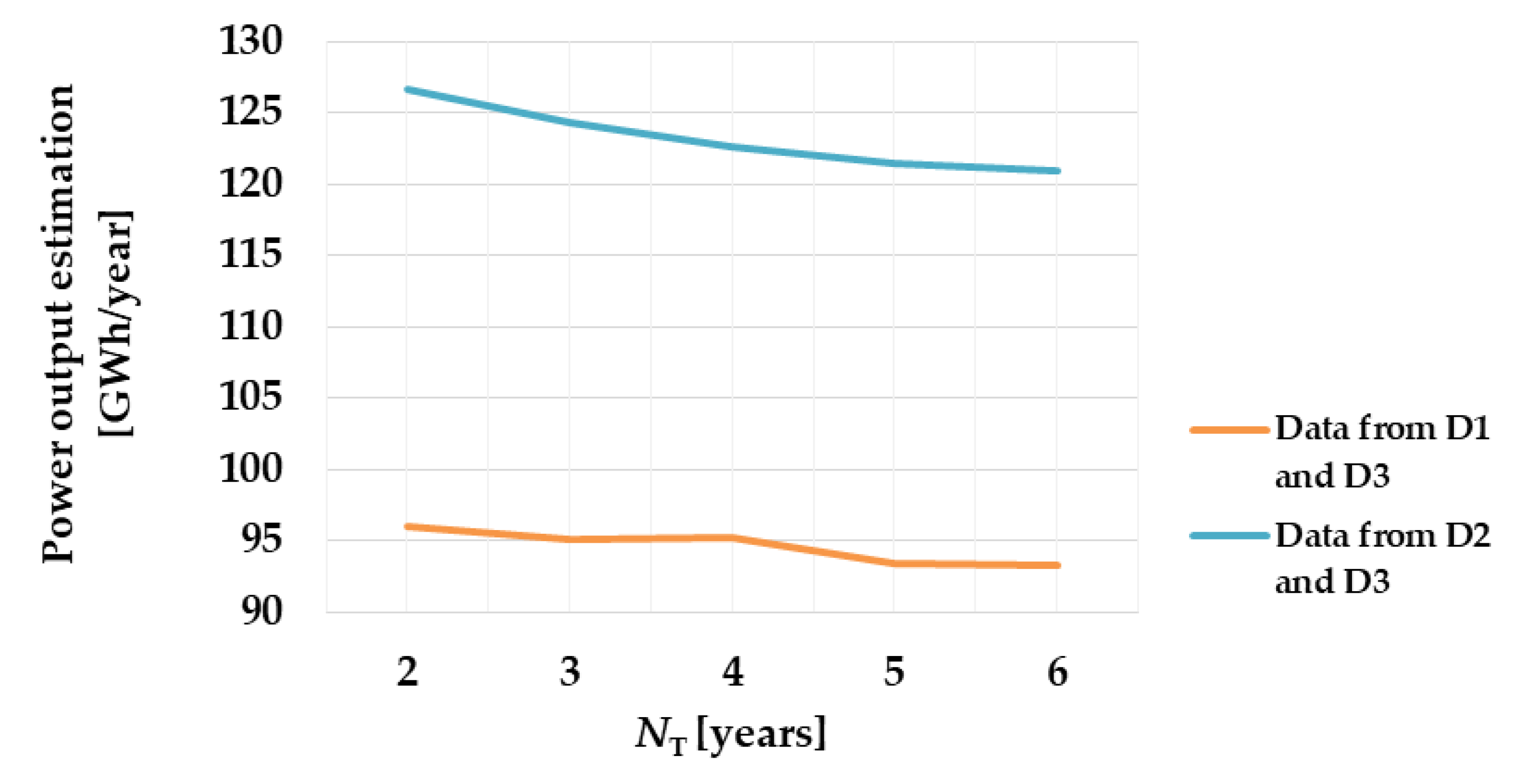
Figure 6.
The values in
Table 7 and
Figure 6 allow concluding that the increase in the duration of the wind monitoring campaign caused the reduction in the estimated quantity of energy to be generated by the hypothetical wind farm in all the cases analyzed. Consequently, the capacity factors would also decrease. These results reflect that longer periods of wind data collection can be more representative of the yearly variability each wind regime is susceptible to.
Conversely, the reduction of the historical uncertainty—and thus the overall uncertainty—acts in the opposite direction, since its isolated effects reflect on the increase of the estimated quantity of energy produced. Yet, these effects are overshadowed by those using larger datasets, which can ultimately provide an energy estimation less prone to errors and, thus, more reliable.
4. Conclusions
This study reveals that a wind monitoring campaign contemplating a more extended duration may allow for better interpretation of the variability in the availability of wind resources in a given target location under the application of the MCP technique. Hence, it is possible to reduce the uncertainty related to the historical characterization of the wind regime in that location, contributing to reducing the overall uncertainty of a WRA. Under the conditions of the recent increase from 24 to 36 months in the minimum length of required wind data recording for a wind farm project to participate in an energy auction in Brazil, the uncertainty related to the historical characterization of wind resources for the data used in this research could be reduced by approximately 18%.
This reduction in the uncertainties group contributes to an increase in the power output estimation of a wind farm, due to the lower overall uncertainty value. This sole fact could lead to an overestimation, which, in turn, may affect the financial structure of a wind farm project. Nevertheless, from the data considered for this research, it was shown that bigger datasets implied a reduction in the estimated energy generation by a wind farm, even considering the overall uncertainty reduction.
The acknowledgement of the outcomes that should follow this expansion in the minimum length of the wind measurement campaign, is perceived as an important contribution to the state of the art pervading the WRA. It seems that the recent new Brazilian regulation could help to enhance a WRA, resulting in more accurate, less prone to overestimation, wind power output estimations. It is understandable that, even if an underestimated energy production is generated by the end of the WRA, the electric sector as a whole may benefit when considering its reliability and expected guaranteed power to be delivered to the grid. For that reason, the findings within this paper should support wind power industry stakeholders to grasp the modifications in the Brazilian wind power sector guidelines, hoping it could also influence decision-making among different countries and their power sectors’ regulatory frameworks. Lastly, it is worth mentioning that incrementing the wind monitoring campaign duration implies more expenses to a project; making it not financially healthy to increase the former indefinitely. The optimum duration—considering costs and accurate power generation outputs—is an interesting topic for further discussion.


