Thermally Anisotropic Composites for Improving the Energy Efficiency of Building Envelopes †


Oak Ridge National Laboratory, One Bethel Valley Road, Oak Ridge, TN 37831, USA
*
Author to whom correspondence should be addressed.
†
This manuscript has been authored by UT-Battelle, LLC, under Contract No. DE-AC05-00OR22725 with the U.S. Department of Energy. The United States Government retains and the publisher, by accepting the article for publication, acknowledges that the United States Government retains a non-exclusive, paid-up, irrevocable, world-wide license to publish or reproduce the published form of this manuscript, or allow others to do so, for United States Government purposes. DOE will provide public access to these results of federally sponsored research in accordance with the DOE Public Access Plan (http://energy.gov/downloads/doe-public-access-plan ).
Energies 2019, 12(19), 3783; https://0-doi-org.brum.beds.ac.uk/10.3390/en12193783
Submission received: 9 September 2019
/
Revised: 27 September 2019
/
Accepted: 29 September 2019
/
Published: 5 October 2019
(This article belongs to the Special Issue Building Thermal Envelope)
Abstract
:This article describes a novel application of thermal anisotropy for improving the energy efficiency of building envelopes. The current work was inspired by existing research on improved heat dissipation in electronics using thermal anisotropy. Past work has shown that thermally anisotropic composites (TACs) can be created by the alternate layering of two dissimilar, isotropic materials. Here, a TAC consisting of alternate layers of rigid foam insulation and thin, high-conductivity aluminum foil was investigated. The TAC was coupled with copper tubes with circulating water that acted as a heat sink and source. The TAC system was applied to a conventional wood-framed wall assembly, and the energy benefits were investigated experimentally and numerically. For experimental testing, large scale test wall specimens were built with and without the TAC system and tested in an environmental chamber under simulated diurnal hot and cold weather conditions. Component-level and whole building numerical simulations were performed to investigate the energy benefits of applying the TAC system to the external walls of a typical, single-family residential building.
1. Introduction
Globally, buildings consume about 40% of the total energy, and are responsible for 30% of carbon dioxide emissions [1]. In building envelope systems, thermal management is important from both energy conservation and thermal comfort perspectives [1,2,3]. Thermal management to reduce unwanted heat flows through the opaque building envelope sections (walls, roof, and foundation) has traditionally been done via insulation materials. Alternative methods that have been proposed include thermal mass, solar control and shading, ventilation, etc. [2,3]. Phase change materials (PCMs), used as latent thermal storage technologies, have shown the potential for reductions in envelope-generated heating and cooling loads [4,5], but systematic studies evaluating the benefits of PCMs in large-scale, real building applications are missing. Vacuum insulation panels (VIPs) and aerogels are among the new generation of high-performance insulation materials being investigated for building envelope applications [6,7,8], but suffer from high cost and/or durability-related questions.
This study investigates the feasibility of applying thermal anisotropy [9] for improved thermal management in building envelopes. Unlike isotropic materials, the thermal conductivity of anisotropic materials is different in different directions, enabling preferential heat transfer in one direction compared to another. Thermal anisotropy allows heat to dissipate in a preferential direction, and has been investigated for improved heat dissipation and hot spot remediation in electronics [10,11,12,13]. Suszko and El-Genk [11] numerically investigated thermally anisotropic composite heat spreaders comprised of two 0.5 mm thick copper (Cu) laments separated by a thin (0.25–1.0 mm) layer of graphite to achieve in-plane thermal conductivities of 200–325 W/(mK) and cross-plane conductivities of 5–20 W/(mK). The composite spreaders were predicted to remove up to 429% higher heat than an all-Cu spreader [11]. Conversely, Ren and Lee [13] utilized the high cross-plane conductivity and low in-plane conductivity of holey silicon nanostructures to achieve improved thermoelectric cooling effectiveness compared to high-thermal conductivity bulk silicon.
The goal of the current research was to investigate if preferential heat transfer using thermal anisotropy can be used for a more effective thermal management of building envelopes compared to passive insulation systems. Narayana and Sato [14] and Vemuri and Bandaru [15], among others, proposed that a practical approach to creating anisotropy is to build a stacked composite from macroscopic layers of isotropic materials. The reasoning is that in a composite made of alternating sheets of two materials, the overall conductivity parallel to the layers is the arithmetic mean (AM) of the individual conductivities of the layers, while the overall conductivity perpendicular to the layers is the harmonic mean (HM) of the individual conductivities [15]. Since HM ≤ AM, the resultant composite will exhibit thermal anisotropy, and the degree of anisotropy can be tuned based on the selection of the isotropic materials and their geometric orientation [15].
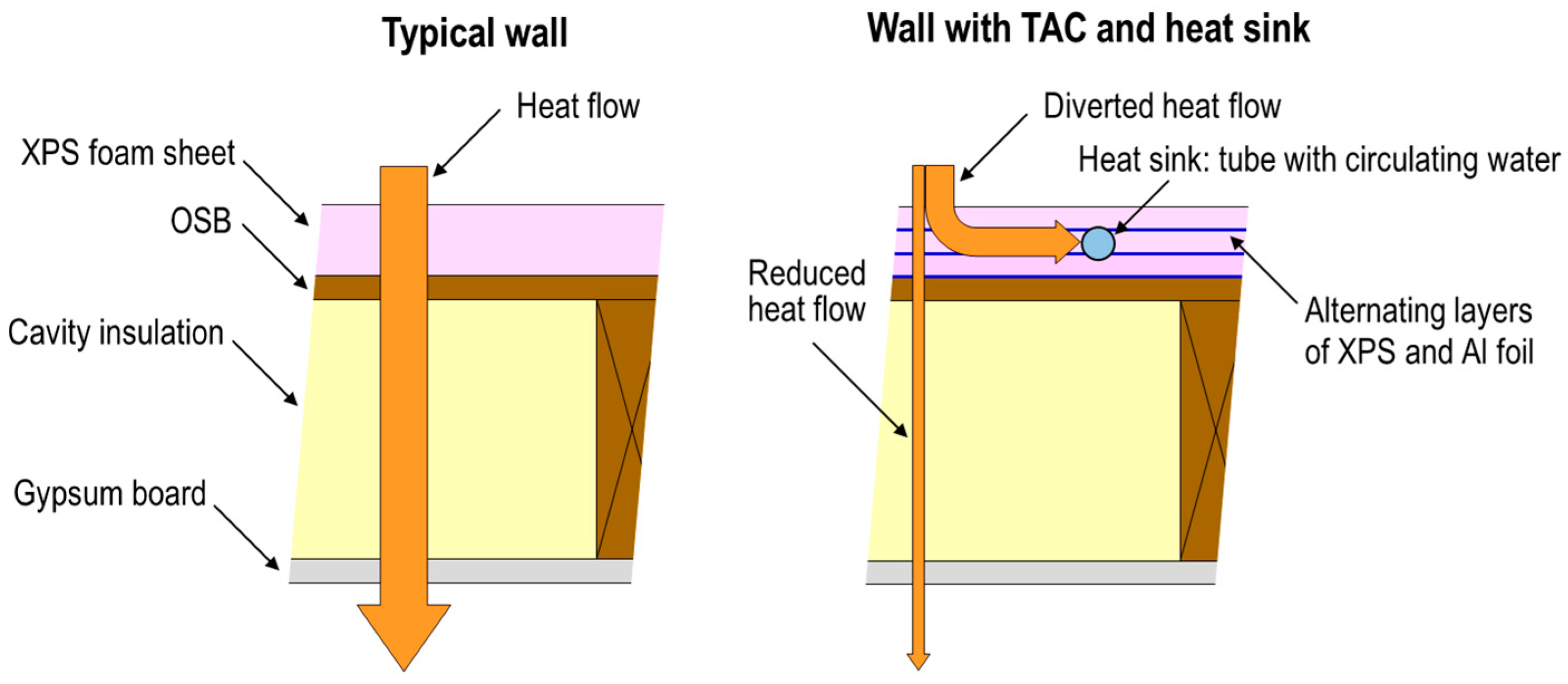
Buildings, as major energy end users, have great potential to relieve the stress of the power surplus/shortage of the electric grid by shifting their loads from on-peak to off-peak periods [16]. Furthermore, with an increasing focus on net-zero energy buildings and stringent future carbon emission targets, envelopes need to switch from passive to dynamic and “responsive” systems [17,18]. For this study, the authors investigated the efficacy of a thermally anisotropic composite (TAC) comprising of alternating layers of rigid extruded polystyrene (XPS) foam sheets and thin aluminum (Al) foil in reducing the heat transfer through a wall system compared to insulation materials alone. The specific TAC materials were chosen because XPS is a commonly used building insulation material, and Al foil is another low-cost, readily available material. In fact, Al foil-faced insulation materials are commercially available. The system design was guided by some preliminary finite element analysis using COMSOL Multiphysics® (https://www.comsol.com/heat-transfer-module) (version 5.4, COMSOL, Inc., Burlington, MA, USA). The Al foil layers were connected to copper (Cu) tubes circulating water that acted as heat sinks and sources, thus providing a dynamic and controllable system. The presence of the Al foils provides very high in-plane conductance compared to the cross-plane conductance across the thickness of the TAC. Figure 1 graphically describes the concept of a TAC diverting heat to a heat sink.
The coupled TAC–heat sink/source concept is promising in terms of reducing energy consumption as well as reducing and/or shifting peak loads. This proof-of-concept research involved experimental evaluations of a full-scale 2.44 × 2.44 m2 wall in an environmental chamber as well as component-level and whole-building simulations to estimate the energy benefits of the TAC combined with heat sinks/sources. The component-level simulations were performed using COMSOL, and the whole-building simulations were performed with EnergyPlus (E+) (https://energyplus.net/).
2. Materials and Methods
2.1. Test Walls, TAC, and Heat Sink/Source
Three test walls were created for testing and evaluation. The baseline (“Base”) test wall consisted of typical wood-framed assemblies that are used in residential buildings in North America. The walls were built with wood studs of 3.8 cm width and 8.9 cm depth that were spaced 0.4 m apart. The wall cavities, i.e., the spaces between the wood studs, were filled with fiberglass insulation and were covered by 1.3 cm thick oriented strand board (OSB) and gypsum board as exterior and interior sheathings, respectively. Next, the baseline wall was upgraded by adding three layers of 1.3 cm thick XPS as exterior insulation to create the “Base + XPS” test wall. Finally, a third test wall (“Base + TAC”) was created by adding the TAC and Cu tubes to the baseline wall. Figure 2 shows a COMSOL-generated schematic of the cross-section of the “Base + TAC” wall. For clarity, only the half-width of the wall is shown.
The TAC consisted of three alternating layers of 1.3 cm thick XPS sheets and 0.13 mm thick Al foil, for a total of six layers. The solid blue lines in Figure 2 indicate the Al foil layers that create the thermal anisotropy and are connected to the Cu tubes, highlighted by the green circles. The external and internal diameter of the Cu tubes were nominally 12.7 mm and 10.9 mm, respectively. Three Cu tubes were installed along alternate wall cavities. Figure 3 shows the physical assembly and construction of the TAC and Cu tubes system. Each Al foil layer was installed and attached to the Cu tubes using Al foil adhesive tape before the corresponding XPS layer was added above. The process was repeated twice to install the three layers each of XPS and Al foil.
2.2. Environmental Chamber and Test Conditions
The experimental evaluations were performed in an environmental chamber called the large scale climate simulator (LSCS). The LSCS consists of three chambers—climate, meter, and guard—as shown in Figure 4. The climate chamber is above ground and simulates outdoor weather conditions of temperature, humidity, irradiance (using infrared or IR lamps), and wind speed. It can maintain steady conditions or simulate diurnal weather conditions. The lower portion of the LSCS contains a guard chamber and a meter chamber. Test specimens are installed at the interface of the climate and meter/guard chambers. The meter chamber is surrounded by the guard chamber on five sides, except for the side facing up, which is exposed to the test specimen. The meter and guard chambers simulate indoor temperature and humidity. The LSCS serves as a guarded hot box apparatus, and tests are performed in accordance with ASTM C1363 [19].
The test wall assemblies were installed horizontally such that their exterior surfaces (OSB or XPS) were exposed to the climate chamber, and their interior surfaces were exposed to the meter chamber. The wall assemblies were supported at the open end of the guard and meter chambers. The meter chamber can be raised and lowered to accommodate the test specimens. During testing, the edge of the meter chamber is sealed against the indoor side of the wall assembly, and provides a measurement of the total heat flow through the 2.44 × 2.44 m2 central measurement area of the test walls. The surrounding guard temperature is maintained close to the meter chamber temperature to minimize heat flows across the meter chamber walls. Thus, the heat flow through the test wall can be calculated from an energy balance of the meter chamber, i.e., the heat input to or removal from the meter chamber to maintain the “indoor” temperature. Reduction in the net heat transfer between the climate and meter chambers was evaluated to prove the efficacy of the proposed TAC with heat sink/source concept.
The climate chamber of the LSCS was programmed to impose a diurnally varying cyclic temperature and IR irradiance on the exterior side of the test wall assemblies. The meter chamber was nominally set to an indoor or “room” condition of 23.9 °C. The heaters, chillers, and fans associated with the meter chamber are controlled to maintain the indoor temperature as near as 23.9 °C as possible, while compensating for the heat gain or loss through the test walls. The walls were instrumented to measure the surface temperatures on the exterior and interior surfaces. For the tests with the TAC walls, a water pump and chiller were used to circulate water through the Cu tubes. The tests were performed under assumed summer and winter environmental conditions. Under summer conditions, the water circulation in the Cu tubes acted as heat sinks with an average inlet water temperature of about 27.8 °C. Under winter conditions, the circulating water acted as heat sources with an average inlet temperature of about 20.5 °C. The sink and source temperatures were based on some preliminary numerical simulations using COMSOL that showed that relatively mild sink/source temperatures can enable significant reductions in heat transfer through the wall.
2.3. Numerical Simulation Methods and Tools
To further evaluate the energy benefits of TACs combined with heat sinks/sources, both component-level and whole building numerical simulations were performed. First, geometries matching the LSCS test walls were created using COMSOL, and model validation simulations were performed. Two-dimensional (2D) geometries were created to match the cross-sections of the different test walls (similar to Figure 2) and utilizing appropriate materials properties, as listed in Table 1. In the “Base” wall model, the OSB was the outmost layer, and the “Base + XPS” wall model only contained the XPS sheets as the exterior insulation. The material properties were obtained from the ASHRAE Handbook of Fundamentals [20], except for the properties of Cu and Al, which were taken from the COMSOL material library.
The model validations were performed using the transient test data from the LSCS. The measured surface temperatures on the exterior wall surface and the meter chamber air temperatures were used as boundary conditions for these simulations. The heat transfer between the interior wall surface and meter chamber air was calculated using a surface heat transfer coefficient (‘hmeter’) for non-reflective horizontal surfaces according to the ASHRAE Handbook of Fundamentals [20]. ‘hmeter’ was 9.26 W/(m2·K) for heat flow in the upward direction, and 6.13 W/(m2·K) for heat flow in the downward direction [20]. The measured and calculated heat flows between the climate and meter chambers were compared to validate the models. For the “Base + TAC” model, the heat sink/source represented by the Cu tubes were modeled using an internal convection heat transfer coefficient (hint) and a mean water temperature. The mean water temperature was based on the measured inlet and outlet water temperatures in the Cu tubes. ‘hint’ was calculated using the following correlation for a laminar, fully developed internal flow under constant heat flux conditions [21].
In Equation (1), ‘D’ is the internal tube diameter, and ‘k’ is the conductivity of the fluid (water). Equation (1) is valid for Reynolds numbers (Re) < 10,000 [21]. For convection heat transfer calculations in internal flows, the assumption of constant heat flux conditions applies to cases where the outer tube surface is uniformly heated or irradiated [21]. This assumption of constant heat flux is deemed reasonable for the current situation, because the exterior surfaces of the test walls were irradiated by an array of uniformly distributed IR lamps.
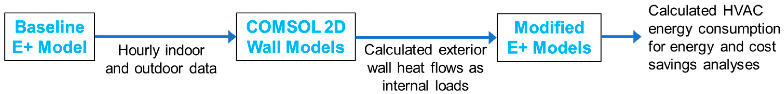
Following the 2D model validation, annual simulations were performed using COMSOL and E+ using typical climate conditions for two US cities, Phoenix, AZ and Baltimore, MD, which lie in climate zones 2 and 4, respectively, according to ASHRAE 90.1 [22]. Figure 5 illustrates the overall modeling and analysis process used for the annual simulations.
The first step of the annual simulation methodology was to build an E+ baseline whole building model, based on a residential prototype building model [23]. The building used for this analysis is a wood-framed, two-story single-family detached house with a total conditioned floor area of about 223 m2. The baseline whole-building E+ model was simulated to generate the indoor and outdoor boundary conditions for the 2D COMSOL models, based on the climate conditions of Phoenix and Baltimore. The exterior surface boundary condition included the impacts of solar irradiance as well as convection and radiation heat transfer with the outdoor environment. The internal boundary conditions included convection and radiation heat transfer with the interior space. The room temperatures for both Phoenix and Baltimore were assumed to be within the heating and cooling set points of 22.2 °C and 23.9 °C, respectively, from the residential prototypes model. The parameters of outdoor and indoor temperatures, solar irradiance, and exterior and interior convection coefficients were generated from the baseline E+ model. An assumption was made that exterior and interior heat transfer coefficients are independent of the wall construction. This is a reasonable approximation based on the research team’s experience with whole-building simulations, which has shown that wall construction has a trivial impact on the calculated surface heat transfer coefficients.
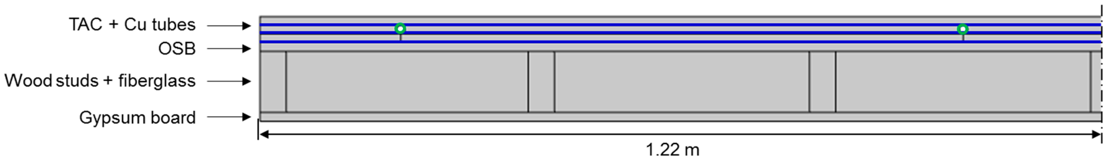
Next, the simplified 2D COMSOL models were used to calculate the wall-generated heating and cooling loads from the “Base”, “Base + XPS”, and “Base + TAC” wall configurations. Figure 6 shows the simplified 2D model of the cross-section of the “Base + TAC” wall for the annual simulations. The simplified models include only two wall cavities and symmetric boundary conditions, i.e., the model assumes that the geometry is repeated symmetrically on either side. The wall components and properties were the same as the 2D validation models.
In the “Base + TAC” model, a Cu tube was assumed to be installed along the center of one of the two modeled wall cavities, same as the LSCS test wall. The internal convection coefficient within the tube was calculated using Equation (1). The Cu tubes were assumed to switch between heat sinks and heat sources during cooling and heating periods, respectively. The mean water temperature was assumed to be 27.8 °C in heat sink mode and 20 °C in heat source mode. For the current work, the switch from heat sink to heat source was assumed when the outdoor ambient temperature fell below 12.8 °C and vice versa. For this study, 12.8 °C was assumed to be the balance point temperature (BPT) for the modeled building. The BPT varies based on building and climate conditions [24], but 12.8 °C is deemed a suitable approximation for the current proof-of-concept simulations.
Finally, the hourly heat flows between the walls and the indoor space calculated from COMSOL were inserted into modified residential prototype E+ models as internal loads. The residential prototype building model used for the E+ simulations was a single-family detached house that complied with International Energy Conservation Code (IECC) 2006. The coefficient of performance (COP) of the cooling system was assumed to be 3.97 at standard design conditions. A gas furnace was modeled to provide heating, and the gas burner efficiency is assumed to be 0.78.
The E+ models were modified to make the opaque wall sections adiabatic, while the other aspects of the prototype models remained the same. The COMSOL-calculated heat gains and losses through the 2D model of the opaque wall sections were treated as cooling and heating loads to the corresponding conditioned space, respectively, in the modified E+ models. This modification was necessary, as E+ utilizes a one-dimensional conduction heat transfer for wall assemblies, and it is not possible to capture the 2D nature of the directional heat flows in the TAC in E+. Thus, this modified approach was used to calculate the heat flows through the opaque wall sections using 2D COMSOL models, and then incorporate them within modified E+ models as wall-generated cooling or heating loads to evaluate the energy benefits of using TACs.
3. Results
3.1. LSCS Experimental Evaluations
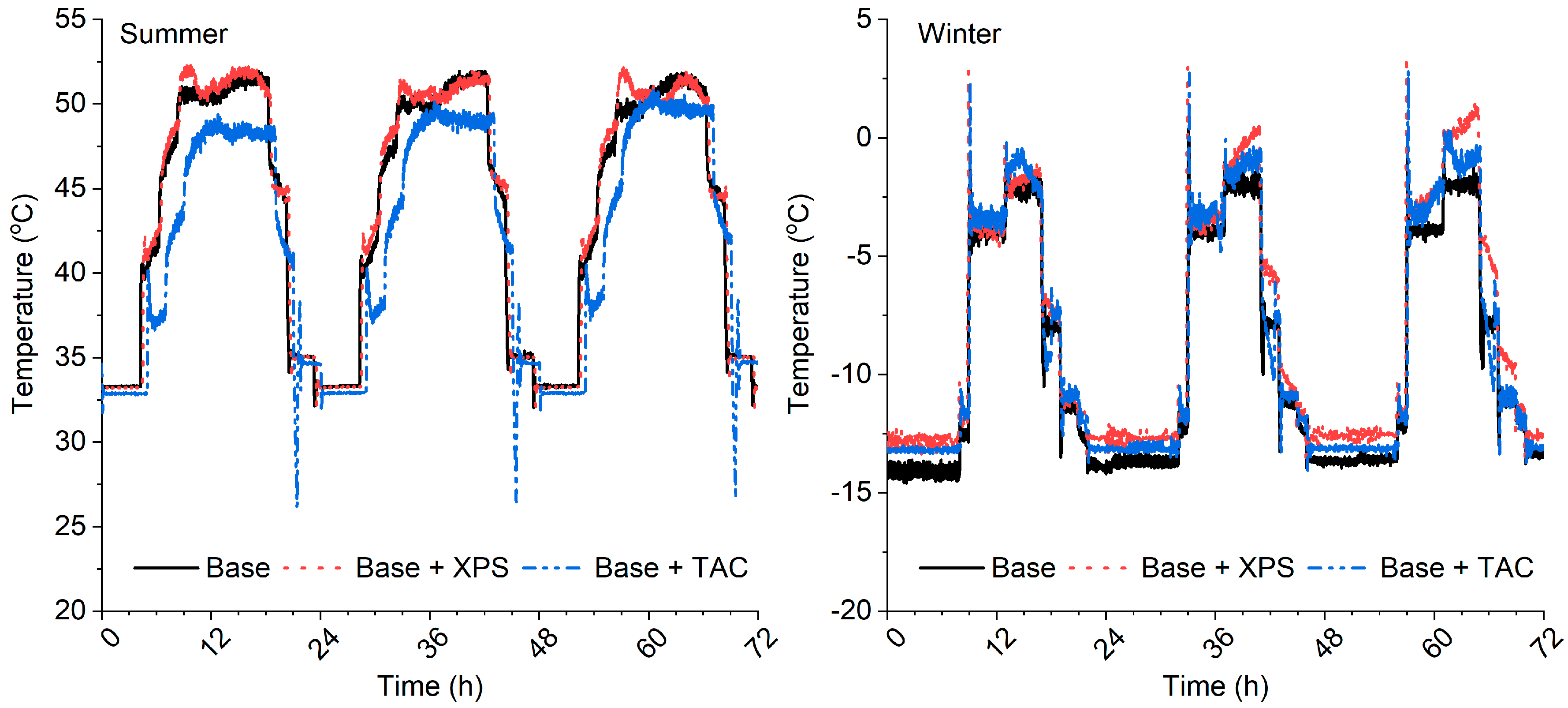
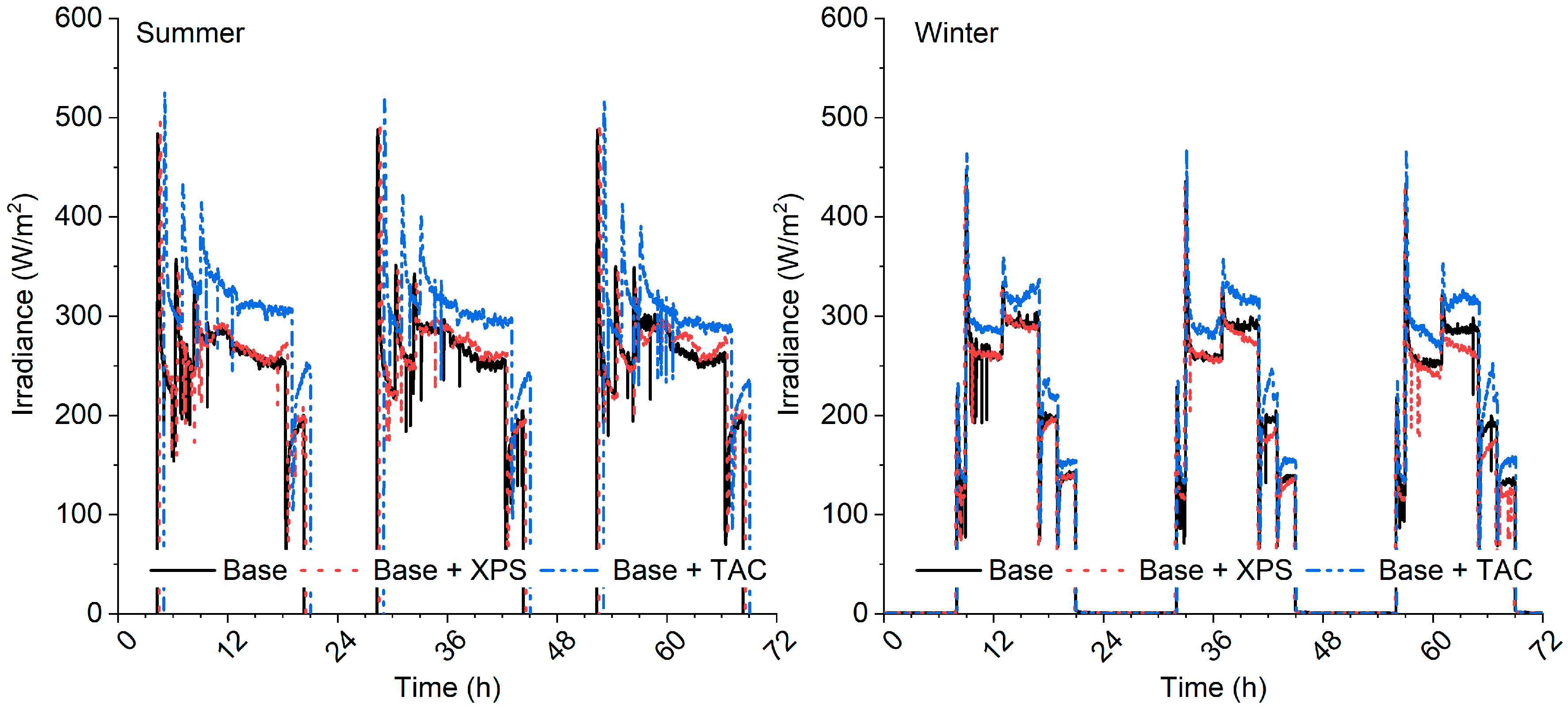
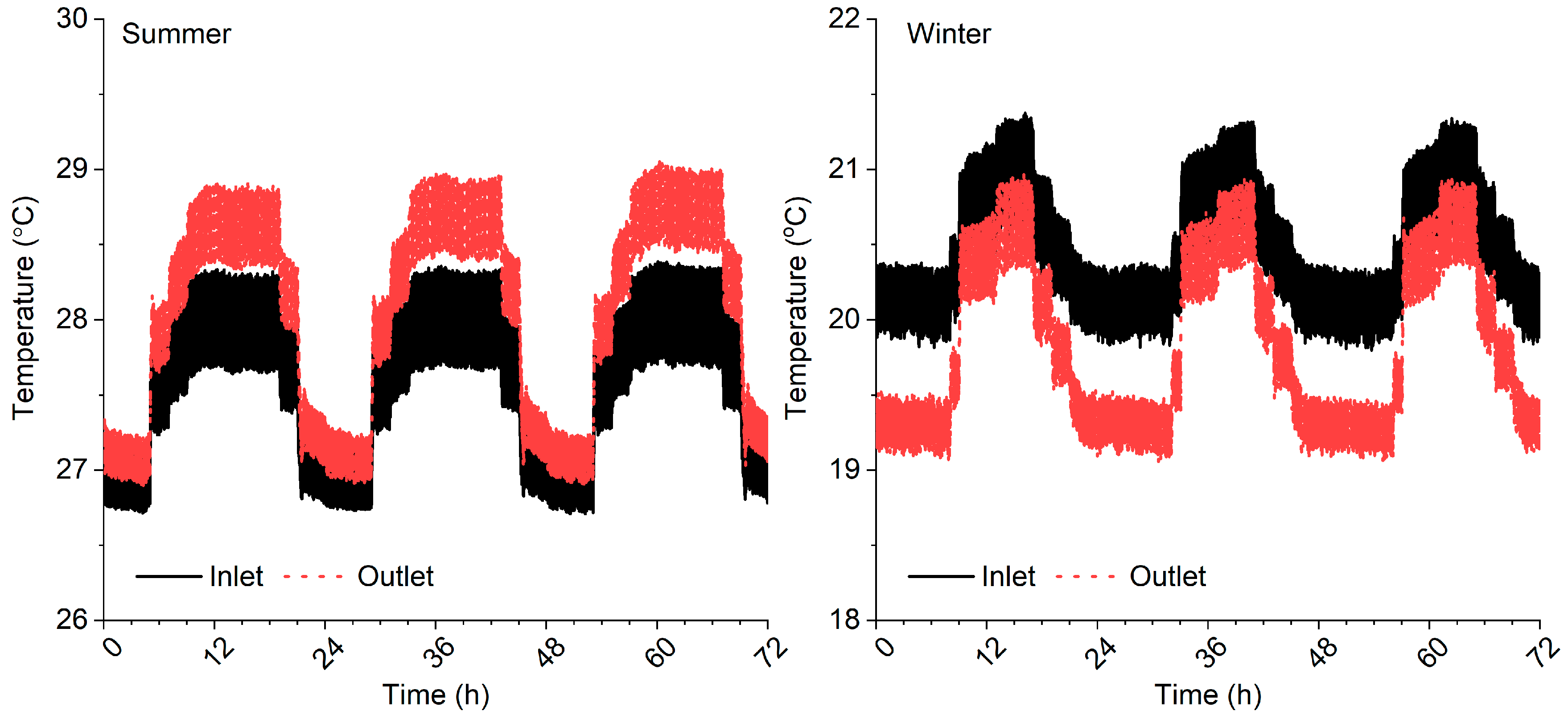
The climate chamber conditions were programmed to create 24-h diurnal cycles of air temperature and IR irradiance (IRR) for assumed summer and winter conditions. The goal of these proof-of-concept tests was to demonstrate the potential of TAC to reduce the heat transfer through the test wall. Each test was performed over multiple diurnal cycles, and data from 72 h (or three 24-h cycles) were used for evaluation and comparison. Figure 7 and Figure 8 show the diurnally varying climate chamber air temperature and the IRR on the exterior surfaces, respectively, of the test walls for the assumed summer and winter conditions. The LSCS was programmed to create the same diurnal conditions for the three test walls as much as possible, but some differences were observed between the different test walls. Figure 9 shows the average inlet and outlet temperatures of the water circulating through the three Cu tubes in “Base + TAC” wall. The water circulation rate varied between 0.053 and 0.057 kg/s through each Cu tube.
Finally, Figure 10 shows the net heat transfer between the climate and meter chamber through the different test walls, which is measured by the net heating or cooling power (Qmeter) needed to maintain the meter chamber at or near the “room” temperature of 23.9 °C. A positive Qmeter indicates net heat flow from the climate to meter chamber (heat gain) or a cooling load, while negative Qmeter indicates heat loss from the meter chamber or a heating load. Figure 10 clearly shows the effectiveness of the TAC and heat sink/source system in reducing both peak cooling and peak heating loads compared to both the baseline wall and “Base + XPS” wall. Under summer conditions, the peak cooling loads were reduced by 43.4% with the “Base + XPS” wall and by 79.5% with the “Base + TAC” wall compared to the “Base” wall. Under winter conditions, the reductions in peak heating loads were 42.1% and 63.7% with the “Base + XPS” and “Base + TAC” walls, respectively.
Table 2 compares the integrated cooling and heating loads over the 72-h summer and winter periods as well as the percent reductions in the loads with the addition of XPS only and the TAC + heat sink/source system to the baseline wall. The LSCS test results showed that using thermal anisotropy combined with a heat sink and sources can significantly outperform insulation materials of similar thickness. Under summer conditions, “Base + TAC” doubled the decrease in cooling loads compared to “Base + XPS”; under winter conditions, “Base + TAC” increased the reduction in heating loads by 40% compared to “Base + XPS”. A future task is to include the energy penalty due to water circulation in the performance evaluation of the “Base + TAC” wall. However, given the low flow rates and mild water temperatures utilized, the energy penalty is expected to be low.
3.2. COMSOL Validation Results
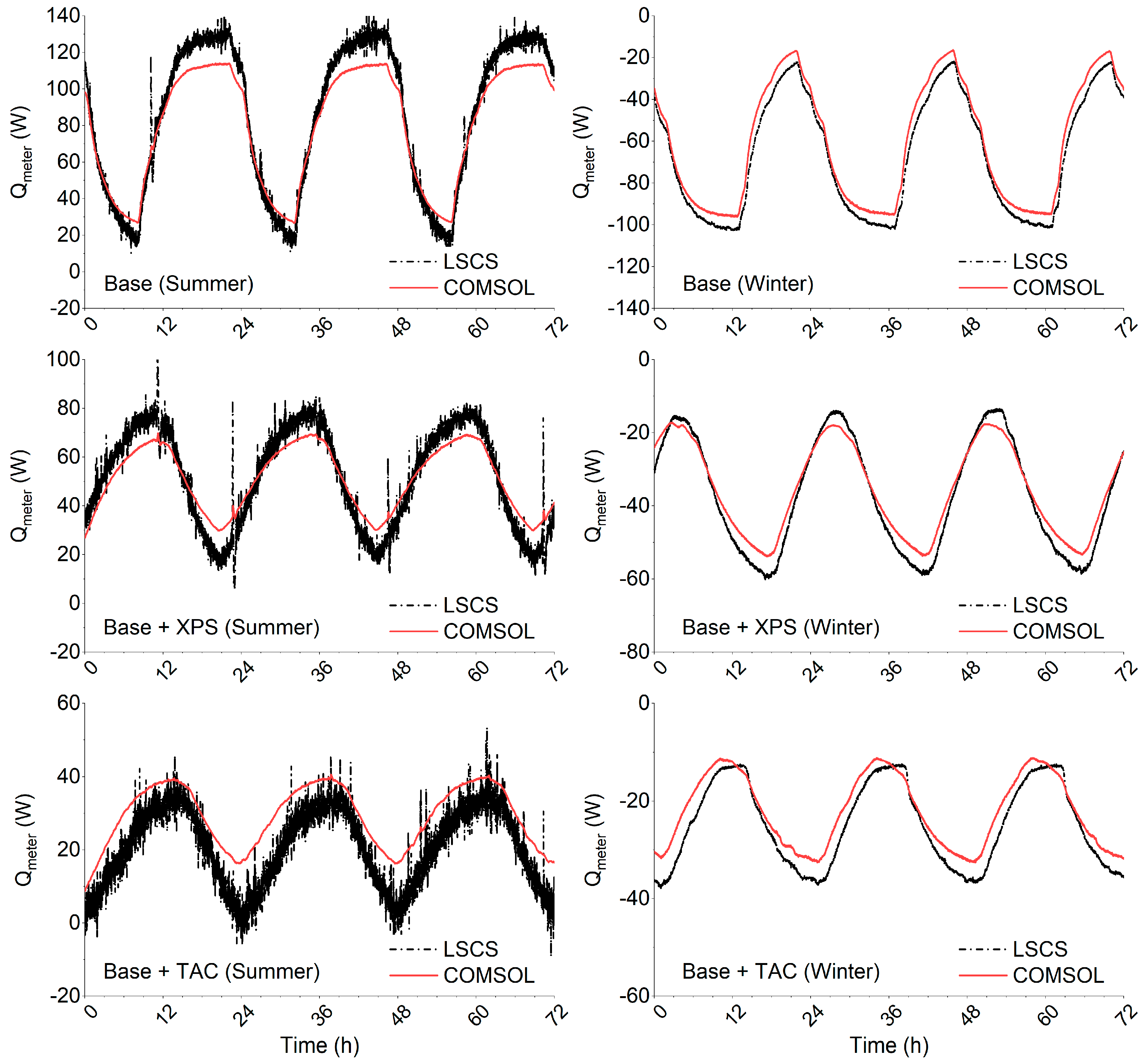
The 2D models matching the test wall cross-sections were created, and the simulated heat flows through the test walls were compared to the LSCS measurements. Figure 11 compares the calculated heat flows through the different test walls with the LSCS measurements. For all cases, the measured exterior surface temperatures of the test walls and meter chamber air temperatures were used as the boundary conditions. The meter-facing or interior surface heat transfer was calculated using ‘hmeter’ of 6.13 W/(m2·K) for summer conditions (heat flow downwards from climate to meter chamber) and 9.26 W/(m2·K) for winter conditions (heat flow upwards from meter to climate chamber). For the “Base + TAC” summer and winter cases, transient ‘hint’ values were calculated using Equation (1). With the flow rates of 0.053–0.057 kg/s and the interior Cu tube diameter of 10.9 mm, the resultant Reynolds numbers were in the range 6200–8200. The ‘k’ of water was obtained from the average of the inlet and outlet temperatures of the water circulating in the Cu tubes. As shown in Figure 9, the difference between the inlet and outlet temperatures were about 1 °C or less, so using an average temperature for ‘hint’ calculations is reasonable. The resultant values of ‘hint’ were 240–246 W/(m2·K).
Overall, the 2D models were able to capture the thermal behavior of all the walls under both summer and winter conditions. Under summer conditions, the calculated peak cooling loads were within 11% of the measurements for the “Base” and “Base + XPS” cases, and within 15% for the “Base + TAC” case. Under winter conditions, the calculated peak heating loads were within 6%, 8%, and 11% of the measurements for the “Base”, “Base + XPS”, and “Base + TAC” cases, respectively.
3.3. Annual Simulation Results
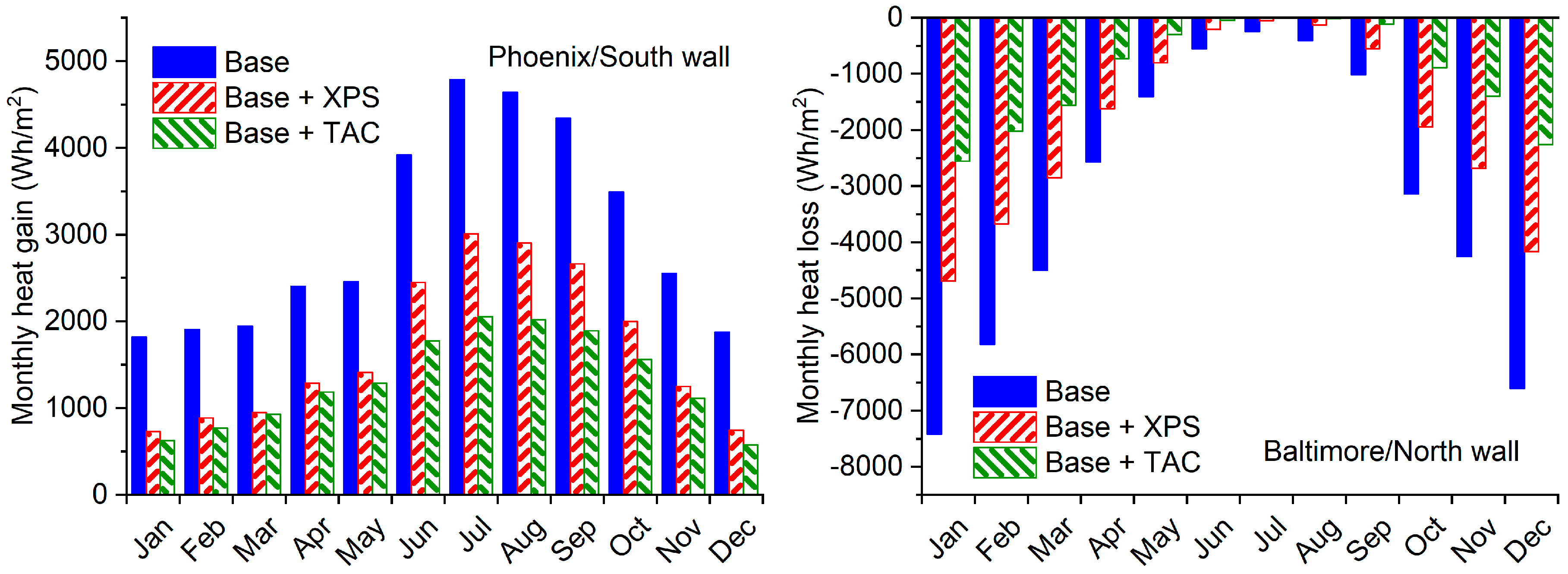
The annual simulations were based on typical weather conditions in Phoenix and Baltimore; the former is in a cooling-dominated climate zone, and the latter has a heating-dominated climate. For the simplified 2D COMSOL models, the exterior and interior boundary conditions were generated using E+ simulations of the residential prototype building model [23]. For the “Base + TAC” model, a flow rate of 0.056 kg/s was assumed in the Cu tube, and the water temperature was assumed to be 27.8 °C in the heat sink mode and 20.0 °C in the heat source mode. The resultant ‘hint’ for the heat sink and heat source modes were 245.7 and 241.2 W/(m2·K), respectively. The switch between heat sink and heat sources happened when the outdoor temperature went above or below the assumed BPT of 12.8 °C. Hourly heat flows through the opaque wall sections were calculated from the 2D COMSOL models and used as cooling and heating loads in the modified E+ models with the adiabatic walls. COMSOL simulations were performed for walls oriented in all four cardinal directions—north, east, south, and west. Figure 12 shows a comparison of the integrated monthly heat gains through a south-facing wall in Phoenix and monthly heat losses through a north-facing wall in Baltimore. Table 3 presents the calculated annual heat gains and losses for the different cases.
In addition to the reductions in overall heat gains and losses, the potential of the ‘Base + TAC’ case to reduce and shift peak loads was also explored. Table 4 lists the COMSOL-calculated average reduction in peak heat gains and average time shift in the peak heat gains in Phoenix during the month of July with the ‘Base + XPS’ and ‘Base + TAC’ cases compared to the ‘Base’ case. While both the ‘Base + XPS’ and ‘Base + TAC’ cases showed similar potential for peak load shifting, the reduction in peak loads was much higher with the ‘Base + TAC’ case.
It should be noted that all heat gains for real buildings don’t directly translate to cooling energy consumption and vice versa for heat losses. For example, heat gains during winter can reduce heating energy consumption without adding to cooling energy use. Therefore, whole building simulations are needed. Using the COMSOL-calculated hourly wall heat flows for the different wall configurations, E+ simulations were performed to estimate their impacts on whole-building cooling and heating energy consumption. Table 5 lists the E+ calculated cooling, heating, and fan energy use for the different wall configurations. The percent reductions in energy use are smaller than the reductions in heat flows, which is expected because overall energy use is also impacted by heat flows through other envelope sections (for example, roofs and windows), indoor loads, etc. In general, the “Base + TAC” case provided greater reductions in energy use than the “Base + XPS” case, except for the cooling energy use in Baltimore. It should be noted that the operating parameters chosen for the “Base + TAC” case for the current simulations were not optimized. Further investigations are ongoing for tuning the TAC and heat sink/source configuration, heat sink/source temperatures, etc., to maximize the peak load reductions and/or energy savings with TACs.
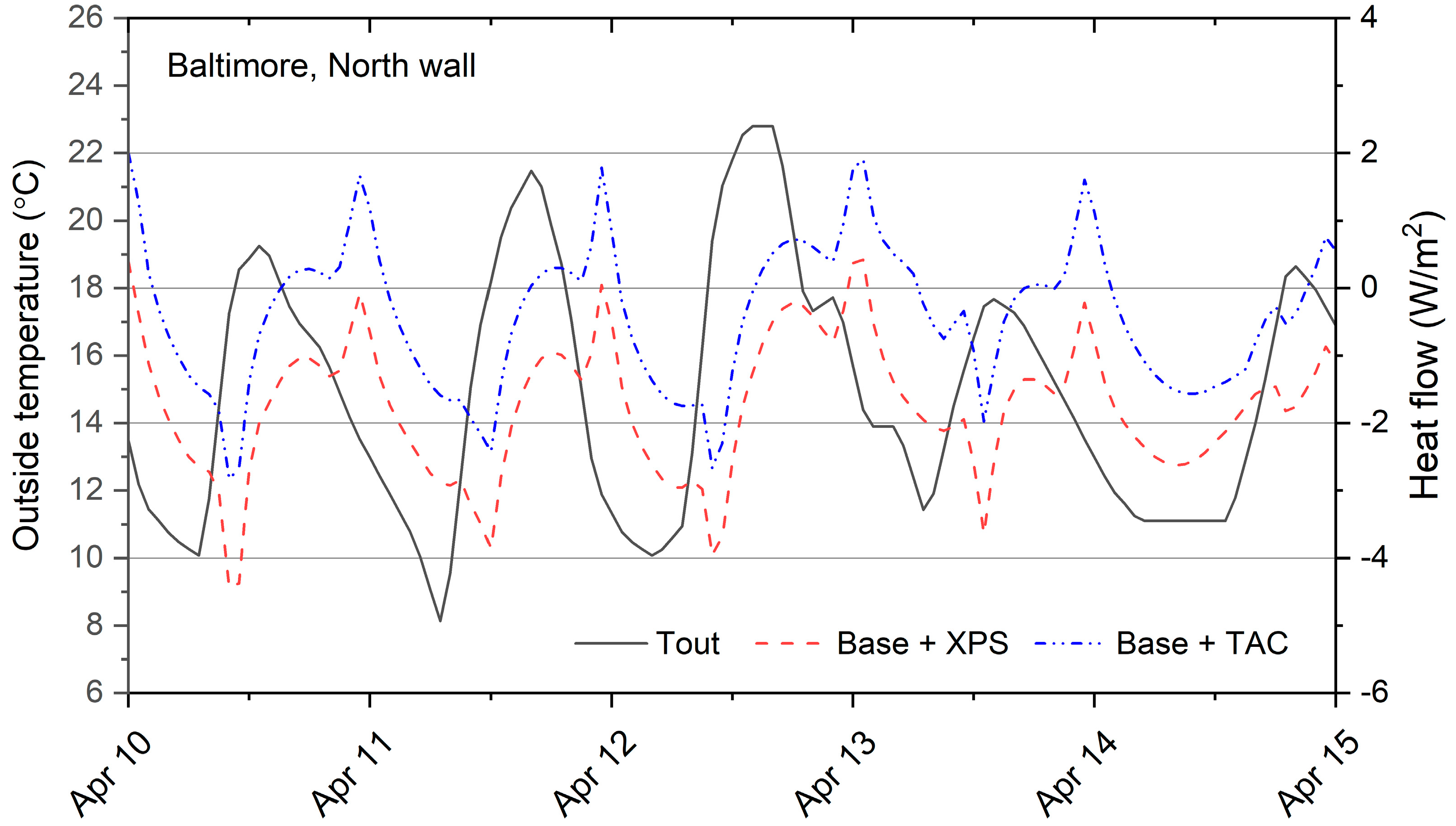
The annual simulation presented here was done to support the proof-of-concept work and show the potential of TACs coupled with heat sink/source to reduce wall-generated heating and cooling loads. The simulation controls and algorithm have not been optimized yet. In Table 3 and Table 4, it is observed that under Baltimore weather conditions, the ‘Base + XPS’ case is more effective at reducing the heat gains and cooling energy use compared to ‘Base + TAC’. For the ‘Base + TAC’ case, it was assumed that the water circulation is always on, and the switch between heat sink and heat source happens when the outdoor temperature crosses 12.8 °C. This can lead to scenarios when the outdoor temperature is lower than the room temperature (22.2–23.9 °C) but greater than 12.8 °C, so the circulating water is assumed to be at 27.8 °C. Thus, during these times, there is a greater temperature gradient for inward heat flow with the ‘Base + TAC’ case compared to the ‘Base + XPS’ case. Figure 13 shows a five-day period in April, when the outdoor temperature (‘Tout’) was predominantly lower than the room temperature but higher than 12.8 °C. As seen from the calculations, there were no heat gains (i.e., heat flows greater than zero) through the ‘Base + XPS’ wall, but there were significant heat gains through the ‘Base + TAC’ wall due to the water circulation at 27.8 °C.
The preliminary annual simulations utilized a simple binary approach to switch between heat sink and source based on a single, constant outdoor temperature value. This was deemed reasonable for this proof-of-concept work. However, a more logical approach would be to use the exterior wall surface and interior temperatures to control the switching between heat sink and source modes, and even turn off the water circulation at times. Such algorithms that would maximize the benefits of the TAC system are being developed, and those results will be published in the near future.
4. Conclusions and Future Work
Here, the development and implementation of a novel TAC-based active envelope system is described. The potential of a TAC to reduce heat flows through building envelopes was experimentally and numerically investigated. A TAC coupled with a heat sink/source was shown to be more effective in reducing both cooling and heating loads and peak cooling loads compared to foam insulation of the same thickness. The TACs consisted of alternating layers of foam insulation and aluminum foil, both of which are commonly available materials. The TAC was connected to copper tubes circulating water for the experimental evaluations, and were able to reduce cooling and heating loads by 86% and 63% compared to a baseline wall with only cavity insulation. Preliminary numerical simulations were performed under two different climate conditions, cooling-dominated and heating-dominated. The TAC system was predicted to reduce cooling energy use by 11% under cooling-dominated climate and heating energy use by 21% in the heating-dominated climate.
The current study was a proof-of-concept investigation. Further optimization of the TAC system is needed to maximize its benefits with respected to peak load reduction and shifting, as well as overall reduction in heating and cooling energy use. By actively controlling the heat sink/source, the building envelope can be tuned to interact with the electric grid and provide benefits to the energy suppliers via peak load reduction and load shifting. The algorithm to switch between heat sink and source as well as turning off the water circulation will be optimized for different building and climate types to maximize the benefits of the TAC system. Finally, the energy penalty of creating a heat sink and source will also be considered.
Author Contributions
K.B. was primarily responsible for creating this manuscript. D.H., K.B., and S.S. developed the preliminary concept of thermal management using anisotropy. K.B. performed the COMSOL simulations. S.S. developed the coupled COMSOL and E+ simulation methodology and performed the E+ simulations. K.B., S.S. and J.A. were jointly responsible for the overall experimental design, testing and data analysis. S.S., D.H. and K.B. were responsible for acquiring funding support for this research.
Funding
This work was funded by the Building Technologies Office (BTO) of the US Department of Energy (DOE), under Contract No. DE-AC05-00OR22725. We gratefully acknowledge the support from Sven Mumme, the responsible Technology Manager of the DOE’s BTO.
Acknowledgments
The authors would like to acknowledge the contribution of Daniel Howard, a post-Bachelor researcher at ORNL, who created the updated graphic for Figure 4.
Conflicts of Interest
The authors declare no conflict of interest.
References
- Yang, L.; Yan, H.; Lam, J.C. Thermal comfort and building energy consumption implications—A review. Appl. Energy 2014, 115, 164–173. [Google Scholar] [CrossRef]
- Sadineni, S.B.; Madala, S.; Boehm, R.F. Passive building energy savings: A review of building envelope components. Renew. Sustain. Energy Rev. 2011, 15, 3617–3631. [Google Scholar] [CrossRef]
- Bhamare, D.K.; Rathod, M.K.; Banerjee, J. Passive cooling techniques for building and their applicability in different climatic zones-The State of Art. Energy Build. 2019, 198, 467–490. [Google Scholar] [CrossRef]
- Kosny, J.; Fallahi, A.; Shukla, N.; Kossecka, E.; Ahbari, R. Thermal load mitigation and passive cooling in residential attics containing PCM-enhanced insulations. Sol. Energy 2014, 108, 164–177. [Google Scholar] [CrossRef]
- Biswas, K.; Shukla, Y.; Desjarlais, A.; Rawal, R. Thermal characterization of full-scale PCM products and numerical simulations, including hysteresis, to evaluate energy impacts in an envelope application. Appl. Therm. Eng. 2018, 138, 501–512. [Google Scholar] [CrossRef]
- Baetens, R.; Jelle, B.P.; Thue, J.V.; Tenpierik, M.J.; Grynning, S.; Uvslokk, S.; Gustavsen, A. Vacuum insulation panels for building applications: A review and beyond. Energy Build. 2010, 42, 147–172. [Google Scholar] [CrossRef] [Green Version]
- Baetens, R.; Jelle, B.P.; Gustavsen, A. Aerogel insulation for building applications: A state-of-the-art review. Energy Build. 2011, 43, 761–769. [Google Scholar] [CrossRef]
- Biswas, K. Development and Validation of Numerical Models for Evaluation of Foam-Vacuum Insulation Panel Composite Boards, Including Edge Effects. Energies 2018, 11, 2228. [Google Scholar] [CrossRef]
- Termentzidis, K. Thermal conductivity anisotropy in nanostructures and nanostructured materials. J. Phys. D-Appl. Phys. 2018, 51, 094003. [Google Scholar] [CrossRef]
- Huang, S.R.; Bao, J.; Ye, H.; Wang, N.; Yuan, G.J.; Ke, W.; Zhang, D.S.; Yue, W.; Fu, Y.F.; Ye, L.L.; et al. The Effects of Graphene-Based Films as Heat Spreaders for Thermal Management in Electronic Packaging. In Proceedings of the 17th International Conference on Electronic Packaging Technology, Wuhan, China, 16–19 August 2016; pp. 889–892. [Google Scholar]
- Suszko, A.; El-Genk, M.S. Thermally anisotropic composite heat spreaders for enhanced thermal management of high-performance microprocessors. Int. J. Therm. Sci. 2016, 100, 213–228. [Google Scholar] [CrossRef]
- Cometto, O.; Samani, M.K.; Liu, B.; Sun, S.X.; Tsang, S.H.; Liu, J.; Zhou, K.; Teo, E.H.T. Control of Nanoplane Orientation in voBN for High Thermal Anisotropy in a Dielectric Thin Film: A New Solution for Thermal Hotspot Mitigation in Electronics. ACS Appl. Mater. Interfaces 2017, 9, 7456–7464. [Google Scholar] [CrossRef] [PubMed]
- Ren, Z.Q.; Lee, J. Thermal conductivity anisotropy in holey silicon nanostructures and its impact on thermoelectric cooling. Nanotechnology 2018, 29, 045404. [Google Scholar] [CrossRef] [PubMed]
- Narayana, S.; Sato, Y. Heat Flux Manipulation with Engineered Thermal Materials. Phys. Rev. Lett. 2012, 108, 214303. [Google Scholar] [CrossRef] [PubMed]
- Vemuri, K.P.; Bandaru, P.R. Geometrical considerations in the control and manipulation of conductive heat flux in multilayered thermal metamaterials. Appl. Phys. Lett. 2013, 103, 133111. [Google Scholar] [CrossRef] [Green Version]
- Xue, X.; Wang, S.W. Interactive Building Load Management for Smart Grid. In Proceedings of the 2012 Power Engineering and Automation Conference, Wuhan, China, 14–16 September 2012; pp. 371–375. [Google Scholar]
- Perino, M.; Serra, V. Switching from static to adaptable and dynamic building envelopes: A paradigm shift for the energy efficiency in buildings. J. Facade Des. Eng. 2015, 3, 143–163. [Google Scholar] [CrossRef] [Green Version]
- Lufkin, S. Towards dynamic active facades. Nat. Energy 2019, 4, 635–636. [Google Scholar] [CrossRef]
- ASTM. ASTM C1363-11, Standard Test Method for Thermal Performance of Building Materials and Envelope Assemblies by Means of a Hot Box Apparatus; ASTM International: West Conshohocken, PA, USA, 2011. [Google Scholar]
- ASHRAE. Handbook—Fundamentals. 2013. Available online: https://www.ashrae.org/technical-resources/ashrae-handbook (accessed on 4 October 2019).
- Incropera, F.P.; DeWitt, D.P. Fundamentals of Heat and Mass Transfer, 4th ed.; John Wiley & Sons, Inc.: Hoboken, NJ, USA, 1996. [Google Scholar]
- ANSI/ASHRAE/IES Standard 90.1-2016, in Energy Standard for Buildings Except Low-Rise Residential Buildings; ASHRAE: Atlanta, GA, USA, 2016.
- Residential Prototype Building Models. Available online: https://www.energycodes.gov/development/residential/iecc_models (accessed on 4 October 2019).
- Krese, G.; Lampret, Z.; Butala, V.; Prek, M. Determination of a building’s balance point temperature as an energy characteristic. Energy 2018, 165, 1034–1049. [Google Scholar] [CrossRef]
Figure 1.
Conceptual operation of a thermally anisotropic composite (TAC)–heat sink combination applied to a wall to reduce heat gains during hot outdoor conditions.
Figure 1.
Conceptual operation of a thermally anisotropic composite (TAC)–heat sink combination applied to a wall to reduce heat gains during hot outdoor conditions.

Figure 2.
COMSOL rendering of the schematic cross-section of the “Base + TAC” wall.

Figure 3.
Creating the TAC and Cu tubes system for the test wall. (a) Cu tubes installed above the oriented strand board (OSB) that was covered with a water and vapor resistive membrane, (b) addition of the first Al foil and rigid extruded polystyrene (XPS) layers, (c) second and third XPS layers sandwiching the third Al foil layer, and (d) finished TAC and Cu tubes system.

Figure 4.
Sketch of the large scale climate simulator (LSCS).

Figure 5.
Flowchart illustrating the modeling and analysis process for the annual simulations.

Figure 6.
Simplified 2D COMSOL model used for annual simulation with symmetric boundary conditions at the two edges.
Figure 6.
Simplified 2D COMSOL model used for annual simulation with symmetric boundary conditions at the two edges.

Figure 7.
Air temperature in the climate chamber.

Figure 8.
IR irradiance on the exterior wall surfaces.

Figure 9.
Average inlet and outlet water temperatures in the Cu tubes for the “Base + TAC” tests.

Figure 10.
Measured heat gains to and heat losses from the meter chamber.

Figure 11.
Comparison of measured and calculated heat gains to and heat losses from the meter chamber.
Figure 11.
Comparison of measured and calculated heat gains to and heat losses from the meter chamber.

Figure 12.
Calculated monthly heat gains through a south-facing wall in Phoenix and heat losses through a north-facing wall in Baltimore.
Figure 12.
Calculated monthly heat gains through a south-facing wall in Phoenix and heat losses through a north-facing wall in Baltimore.

Figure 13.
Outdoor temperature (left axis) and calculated heat flows (right axis) through a north-facing wall in Baltimore.
Figure 13.
Outdoor temperature (left axis) and calculated heat flows (right axis) through a north-facing wall in Baltimore.


Table 1.
Material properties used in the simulations.
| Material | Thermal Conductivity [k, W/(m·K)] | Density [ρ, kg/m3] | Specific Heat [cp, J/(kg·K)] |
|---|---|---|---|
| Gypsum | 0.159 | 640.7 | 879.2 |
| Wood stud | 0.144 | 576.7 | 1632.9 |
| Fiberglass | 0.039 | 7.8 | 837.4 |
| OSB | 0.130 | 656.8 | 1884.1 |
| XPS | 0.029 | 32.0 | 1465.4 |
| Aluminum | 238 | 2700 | 900 |
| Copper | 400 | 8960 | 385 |
Table 2.
Comparison of integrated cooling and heating loads.
| Test Parameter | Base | Base + XPS | Base + TAC | |
|---|---|---|---|---|
| Summer | Cooling load (Wh) | 5310 | 3021 | 770 |
| % difference | - | −43.1% | −85.5% | |
| Winter | Heating load (Wh) | 4781 | 2629 | 1760 |
| % difference | - | −45.0% | −63.2% | |
Table 3.
Comparison of calculated annual wall heat gains and losses and percent difference with respect to the “Base” wall.
Table 3.
Comparison of calculated annual wall heat gains and losses and percent difference with respect to the “Base” wall.
| Wall Type | Performance Metric | North | East | South | West |
|---|---|---|---|---|---|
| Phoenix | |||||
| Base | Heat gain (kWh/m2) | 19.0 | 31.6 | 36.1 | 32.4 |
| Base + XPS | Heat gain (kWh/m2) | 11.4 | 18.1 | 20.3 | 18.9 |
| % difference | −40.1% | −42.6% | −43.9% | −41.6% | |
| Base + TAC | Heat gain (kWh/m2) | 10.6 | 14.3 | 15.8 | 14.9 |
| % difference | −44.2% | −54.7% | −56.4% | −53.8% | |
| Base | Heat loss (kWh/m2) | −14.9 | −10.9 | −10.1 | −12.7 |
| Base + XPS | Heat loss (kWh/m2) | −8.9 | −5.7 | −4.2 | −6.3 |
| % difference | −40.0% | −48.1% | −58.8% | −50.3% | |
| Base + TAC | Heat loss (kWh/m2) | −3.6 | −2.5 | −2.2 | −3.1 |
| % difference | −75.8% | −77.0% | −78.1% | −75.6% | |
| Baltimore | |||||
| Base | Heat gain (kWh/m2) | 5.1 | 10.4 | 12.1 | 10.6 |
| Base + XPS | Heat gain (kWh/m2) | 2.6 | 5.1 | 5.2 | 5.4 |
| % difference | −49.3% | −50.7% | −57.1% | −48.8% | |
| Base + TAC | Heat gain (kWh/m2) | 4.2 | 5.7 | 5.9 | 6.0 |
| % difference | −17.6% | −45.2% | −51.1% | −43.3% | |
| Base | Heat loss (kWh/m2) | −37.9 | −32.9 | −30.1 | −34.4 |
| Base + XPS | Heat loss (kWh/m2) | −23.4 | −19.7 | −16.7 | −20.4 |
| % difference | −38.3% | −40.3% | −44.6% | −40.7% | |
| Base + TAC | Heat loss (kWh/m2) | −11.9 | −10.4 | −9.1 | −10.9 |
| % difference | −68.6% | −68.5% | −69.6% | −68.3% | |
Table 4.
Calculated average peak heat gain reduction and average peak shift during July in Phoenix.
| Wall Type | Performance Metric | North | East | South | West |
|---|---|---|---|---|---|
| Base + XPS | Peak reduction (%) | 40.6 | 53.0 | 46.5 | 48.7 |
| Peak shift (h) | 0.7 | 4.0 | 3.8 | 1.2 | |
| Base + TAC | Peak reduction (%) | 58.6 | 69.3 | 63.6 | 66.6 |
| Peak shift (h) | 0.6 | 5.0 | 3.6 | 1.1 |
Table 5.
Comparison of calculated annual whole building cooling and heating-related energy use and percent difference with respect to the “Base” case.
Table 5.
Comparison of calculated annual whole building cooling and heating-related energy use and percent difference with respect to the “Base” case.
| Wall Type | Cooling and Fan Energy Use (kWh) | % Difference | Heating Energy Use (kWh) | % Difference |
|---|---|---|---|---|
| Phoenix | ||||
| Base | 11,278 | - | 4855 | - |
| Base + XPS | 10,268 | −9.0% | 3804 | −21.6% |
| Base + TAC | 9998 | −11.3% | 3342 | −31.2% |
| Baltimore | ||||
| Base | 4158 | - | 21,945 | - |
| Base + XPS | 3801 | −8.6% | 19,244 | −12.3% |
| Base + TAC | 3838 | −7.7% | 17,413 | −20.6% |
© 2019 by the authors. Licensee MDPI, Basel, Switzerland. This article is an open access article distributed under the terms and conditions of the Creative Commons Attribution (CC BY) license (http://creativecommons.org/licenses/by/4.0/).
Share and Cite
MDPI and ACS Style
Biswas, K.; Shrestha, S.; Hun, D.; Atchley, J. Thermally Anisotropic Composites for Improving the Energy Efficiency of Building Envelopes. Energies 2019, 12, 3783. https://0-doi-org.brum.beds.ac.uk/10.3390/en12193783
AMA Style
Biswas K, Shrestha S, Hun D, Atchley J. Thermally Anisotropic Composites for Improving the Energy Efficiency of Building Envelopes. Energies. 2019; 12(19):3783. https://0-doi-org.brum.beds.ac.uk/10.3390/en12193783
Chicago/Turabian StyleBiswas, Kaushik, Som Shrestha, Diana Hun, and Jerald Atchley. 2019. "Thermally Anisotropic Composites for Improving the Energy Efficiency of Building Envelopes" Energies 12, no. 19: 3783. https://0-doi-org.brum.beds.ac.uk/10.3390/en12193783
Note that from the first issue of 2016, this journal uses article numbers instead of page numbers. See further details here.