Forecasting the Price Distribution of Continuous Intraday Electricity Trading

Energy Information Networks & Systems, TU Darmstadt, 64283 Darmstadt, Germany
*
Author to whom correspondence should be addressed.
Energies 2019, 12(22), 4262; https://0-doi-org.brum.beds.ac.uk/10.3390/en12224262
Submission received: 30 August 2019
/
Revised: 4 November 2019
/
Accepted: 5 November 2019
/
Published: 8 November 2019
(This article belongs to the Special Issue Modeling and Forecasting Intraday Electricity Markets)
Abstract
:The forecasting literature on intraday electricity markets is scarce and restricted to the analysis of volume-weighted average prices. These only admit a highly aggregated representation of the market. Instead, we propose to forecast the entire volume-weighted price distribution. We approximate this distribution in a non-parametric way using a dense grid of quantiles. We conduct a forecasting study on data from the German intraday market and aim to forecast the quantiles for the last three hours before delivery. We compare the performance of several linear regression models and an ensemble of neural networks to several well designed naive benchmarks. The forecasts only improve marginally over the naive benchmarks for the central quantiles of the distribution which is in line with the latest empirical results in the literature. However, we are able to significantly outperform all benchmarks for the tails of the price distribution.
1. Introduction
Continuous intraday electricity trading offers market participants the possibility to balance short-term deviations from their planned generation and load schedules. This is especially valuable for agents with a high share of generation from non-dispatchable renewable energy sources like wind and solar. Conventionally, deviations from the day-ahead schedules are compensated through balancing energy which is contracted and centrally dispatched by the transmission system operator. The possibility to trade electricity on short notice can partly explain the counter intuitive situation that the demand for balancing energy in Germany in the last years substantially declined, while at the same time the share of generation from renewable sources increased [1,2]. Thus, intraday markets can be an effective tool to support the transition to a flexible and renewable energy system and have seen steadily growing volumes in recent years [3].
In this work we will focus on the German continuous intraday market. On this market it is possible to trade hourly and quarter-hourly contracts for the delivery of electricity till 30 min before delivery. Inside of the four control zones it is possible to trade until five minutes before the delivery starts. Contrary to the day-ahead auction, the intraday market is operated as a continuous pay-as-bid market, i.e., market participants can submit bids and asks for price-volume combinations which are immediately executed if two offers in the order book can be matched. This results in a potentially large set of prices for the same product. Therefore, price indexes that reflect the volume-weighted average price are a main indicator of market outcomes. The most important one is the ID3 price index which is the volume-weighted average price of all trades in the time interval from three hours before delivery till 30 min before delivery [4]. For a detailed description of the German power markets see [5].
In contrast to the well researched day-ahead markets [6], the literature regarding intraday electricity price forecasting is scarce. Andrade et al. [7] and Monteiro et al. [8] conducted a forecasting study for the Iberian intraday electricity market. However, this market does not resemble the design of the German market. Most importantly, the Iberian intraday market is operated as six separate intraday auctions under a uniform pricing regime. More recently, Maciejowska et al. [9] presented a model that is able to predict the price spread between the German day-ahead auction prices and the corresponding volume-weighted average intraday prices. Finally, Uniejewski et al. [10] and Narajewski & Ziel [11] are to our best knowledge the only two papers that aim to directly forecast ID3 prices. The authors of [11] present evidence that the information available to the market at forecasting time, i.e., three hours before delivery, is already efficiently incorporated by the market participants and therefore the best forecast for the ID3 price is the volume-weighted average price of the most recent 15 min of trading.
Since the intraday market is operated under a pay-as-bid regime, it is possible for market participants to sell or buy contracts at prices that substantially differ from the ID3 price. Furthermore, very different sets of trades can result in the same weighted average price. Therefore, we aim to forecast the entire volume-weighted price distribution instead of only volume-weighted average prices. Note that this distribution is not equivalent to a predictive distribution of the ID3 price, but will often be much wider. Such a forecast is important to enable bidding strategies that use prices away from the ID3 price, e.g., to benefit from especially high or low price offers. To approach our task, we construct empirical cumulative distributions for each trading product in discrete time intervals and describe these distributions using a dense grid of quantiles. This results in a set of multivariate time series of quantile values which non-parametrically approximate the targeted price distributions.
We conduct a forecasting study for the German intraday market in which we aim to forecast the quantiles of the price distribution in the time from three hours to 30 min before delivery. We test several linear regression models as well as a neural network model that accounts for the unique structure of the data. We compare the forecasts from these models to several carefully designed naive benchmark models. Our empirical findings support the evidence in [11], as we are only able to outperform the naive benchmarks by a small margin for the central quantiles. However, the performance of our forecasts for the tails of the distributions improves significantly over the benchmark models.
The remainder of the paper is structured as follows. In Section 2 we describe the data set and preliminary data transformation we apply to obtain the quantiles of the price distributions. We present the linear regression and neural network models as well as a set of naive benchmark models in Section 3 and describe our forecasting strategy along with the employed error measures in Section 4. The empirical findings are discussed in Section 5. We conclude in Section 6.
2. Data Set & Data Transformation
The German intraday market has undergone two relevant regulatory changes in the last several years. First, since July 2017 it is possible to trade until 5 min before delivery inside of the control zones. Second, in October 2018 the Austrian control zone was split from the former German-Austrian market. For our analysis we consider data on the intraday transactions from 1 July 2017 to 31 March 2019 for the German-Austrian market and German market respectively, i.e., we start our analysis after the introduction of the 5 min delivery horizon while the market split occurred during the time frame of our analysis. We assume that the control zone split did not have a substantial impact on prices and liquidity since the German control zones are large compared to the Austrian control zone and cross border trading is still possible. The continuous intraday trading data we use is commercially available from Epex Spot [12]. We will only consider hourly products in our analysis as their traded volume is more than five times larger than the volume of the quarter hour products. We additionally consider corresponding exogenous hourly data regarding day-ahead auction prices as well as forecasted renewable generation and load which is available from ENTSO-E [13].
2.1. Constructing Price Distributions from Intraday Trading Data
The trading data contains all executed trades for hour products to be delivered between 1 July 2017 and 31 March 2019. For this period we define a corresponding set of dates . Each entry in the raw data set corresponds to a single trade i and is comprised of the identifier for the hour and the day of delivery, a timestamp of the trading time that indicates the time left until delivery , the trade volume in , and the price in [14].
Forecasting the data on the level of single trades is likely to be difficult and not necessarily needed for decision making. Hence, one has to aggregate the trading data into a more suitable form that is still able to represent the market’s development in sufficient detail. To this end, the literature has so far focused on analyzing and forecasting volume-weighted average prices [9,10,11] which only provide a highly aggregated representation of the market.
We instead propose to work with the entire volume-weighted price distribution of the trades. Therefore, we compute the volume-weighted empirical cumulative distribution function (VWECDF) over the price p,
denotes the VWECDF for the hour product h on day d between the time and before delivery with . The total volume traded for the product in the given interval
is used to normalize the sum in the VWECDF. The VWECDF in Equation (1) for a given product is computationally represented by an ordered set of the J trades observed in the time interval , where is the empirical quantile and is the corresponding quantile value which is given by the price of trade j. This allows us to estimate quantile values for a specific quantile using linear interpolation if necessary
Using a dense grid of quantiles we then obtain a vector of quantile values
which non-parametrically describes the price distribution of the given product in the time interval defined by and . For this empirical distribution, the values for and correspond to the cheapest and most expensive trades observed.
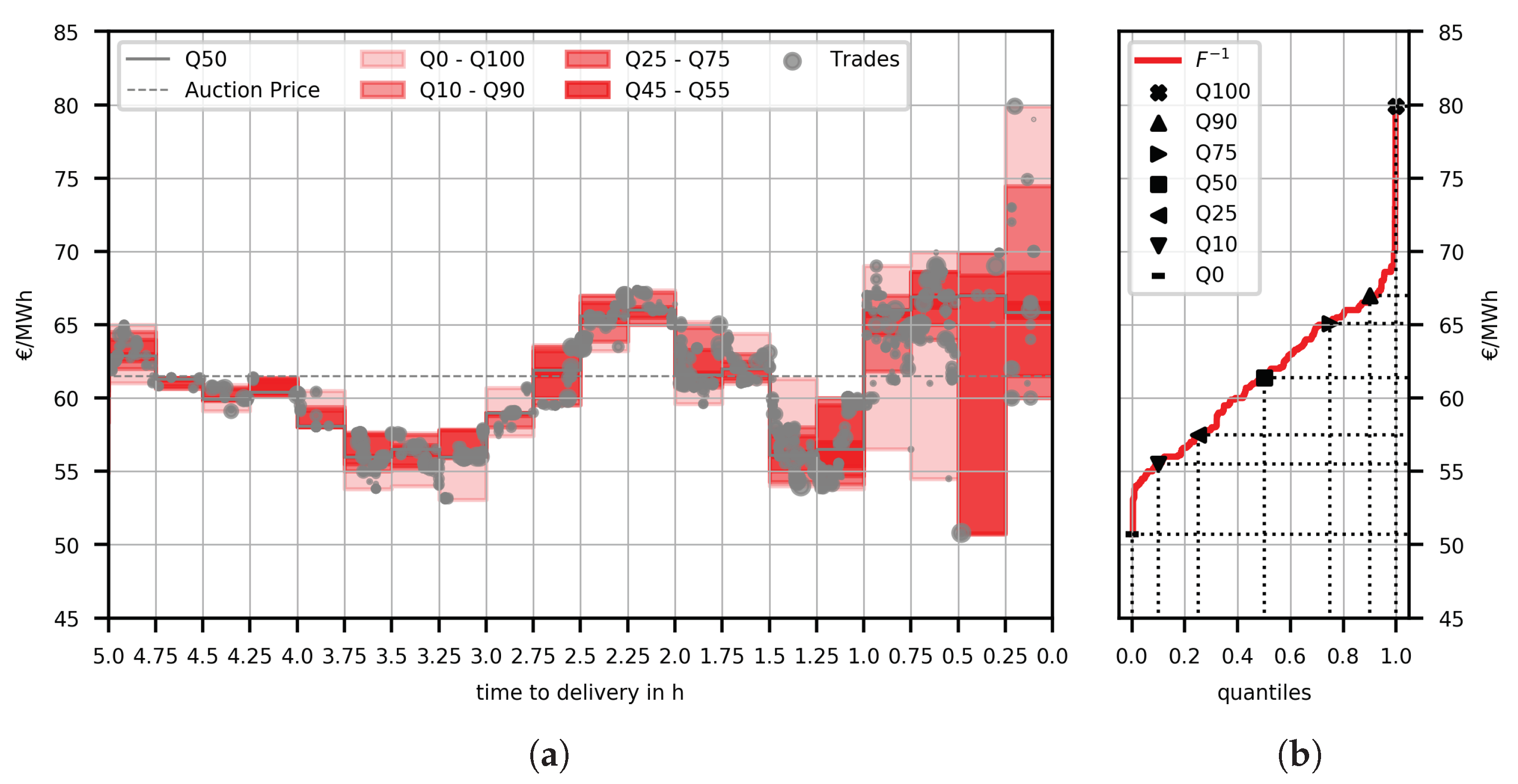
Figure 1a shows the result of the applied transformation in a fan chart for a single product in 15 min time intervals from 5 h before delivery till the time of delivery. We can observe that the variance increases with the time of delivery approaching. This is characteristic for the intraday market. Figure 1b shows the inverse of the VWECDF and quantile values for selected quantiles for the entire time horizon of 5 h.
Let us note again that this is not a distribution which describes the uncertainty over the volume-weighted average price but a distribution that describes how the traded volume is distributed over the possible prices. To illustrate this point consider the following hypothetical situation. Suppose we would observe the trades for a certain product before issuing a forecast for the observed time frame. Then, we could compute the volume-weighted average price and issue a perfect probabilistic forecast for this average price, a distribution where the entire probability mass is centered at the true, known value. However, this forecast would not inform a trader about the variety of prices that are traded for this product. In contrast, our approach would still forecast a non-trivial distribution that would inform an agent about the dispersion of the traded prices, e.g., we could exactly forecast the marginal value of the cheapest and most expensive 10% of the trades. This is a much richer representation of the market behavior and reflects that different market participants might value electrical energy very differently. Considering a price taker perspective, an agent could then take advantage of the estimated dispersion of prices.
2.2. Exogenous Data
Along with the trading data we also include exogenous fundamental data. For each day and hour we consider the load forecast , the forecasted in-feed from wind and solar power , and the day ahead auction price which is already known before the continuous trading starts. We combine all exogenous variables in the vector . Additionally we consider the 24-dimensional one-hot encoded column vector which contains a dummy variable for each hour of the day.
3. Predicting the Quantiles of the Price Distribution
The most important price index for the intraday market is the ID3 price. It is the volume-weighted average price of the trades in the time interval from three hours before delivery till 30 min before delivery for a given product [4]. We therefore also focus on this time horizon and aim to forecast . As explanatory variables we use the time series of the observed quantile values from four to three hours before delivery in 15 min time intervals denoted by , i.e., is a matrix of dimension where is the number of quantiles. We also consider the corresponding time series from the two neighboring products and which are also of dimension . Furthermore, denotes the th column of . For ease of notation we will write to denote the product that has to be delivered k hours before/after the product instead of using the correct notation . Finally, we also use the exogenous variables for all three considered products and the vector of hour dummy variables .
3.1. Linear Regression Models
In this section we present a set of linear regression models which use different subsets of the available regressors. This allows us to stepwise infer the contribution of each factor to the forecasting performance. To obtain a forecast for the vector of quantile values we have to fit a separate model for each quantile . At test time we concatenate the predictions from the individual models and sort the resulting vector to ensure monotonically increasing quantile values.
The first model, which we call AR1, uses only the time series information of the same product for the same quantile and the vector of dummy variables . It is given by
where are row vectors of model parameters. The model ARX1 given by
additionally uses the exogenous variables for the same product. The model AR2 given by
also utilizes the time series information from the neighboring products for the same quantile but ignores the exogenous variables. The model ARX2 given by
additionally includes the exogenous regressors for all three products. Finally the ARXfull model
utilizes all available inputs. Hence, this model has 1245 parameters. This will likely result in overfitting for the used training set size of 6 months. Furthermore, many regressors might not carry useful information for the quantile value to forecast. We therefore apply Lasso regularization to automatically select an optimal subset of regressors [15], i.e., the model parameters are estimated using an extended loss function that penalizes the norm of the model weights. Let be a vector of standardized regressors, the model weights, and the true quantile values, then the Lasso estimator for the optimal weight vector is given by
where is the hyperparameter that controls the degree of regularization. Setting leads to standard ordinary least squares estimation.
3.2. Neural Network Model
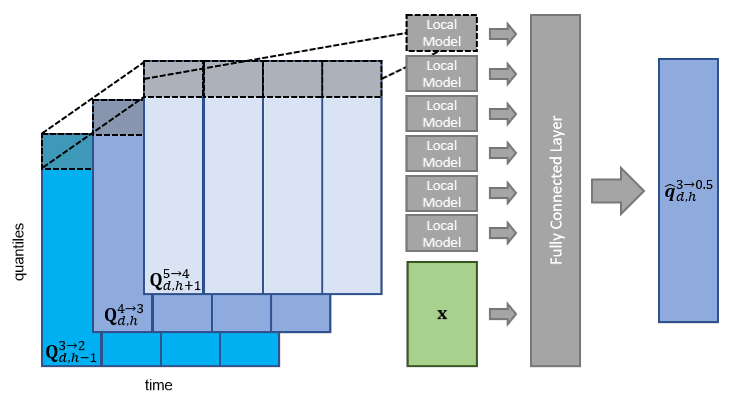
The modeling approaches described above result in one model per quantile and can only model linear relationships. Therefore, we also test a multi output neural network model (NN) which uses an architecture that accounts for the structure of the inputs and limits the number of parameters in the hidden layers, see Figure 2 for a visualization. The model outputs a prediction for the vector of quantile values as a function of all available regressors
The proposed neural network has two hidden layers. The first hidden layer is a locally connected layer and operates only on the time series data . In this locally connected layer a distinct vector of weights is learned for each quantile. Each local model outputs a scalar value
where denotes the th column of . The function
is the ELU activation function [16]. The layer outputs a vector of dimension . The vector is then concatenated with the vectors and is passed through a fully connected layer
with neurons, i.e., the weight matrix has dimension and is a vector of constants with dimension . The last layer
outputs the model’s prediction using the weight matrix and the vector of constants .
We train the model by minimizing the L2 norm of the difference between the predicted and true vector of quantile values given by
where D is the number of days in the training set. We train the model for 50 epochs with a batch size of 32 using the Adam optimizer [17] at standard settings in Keras 2.2.4 [18]. At test time we sort the predictions of the model to ensure monotonically increasing quantile values.
For both the linear regression models as well as the neural network model we chose to use one model for all hours of the day. Fitting a separate model for each hour would result in much smaller training sets. However, if the market behaves fundamentally different for different hour products, it might be insufficient to account for these differences by simply introducing dummy variables. We also did not transform the data to stabilize the variance e.g., by applying the -transformation which has been shown to work well for electricity price forecasting tasks [19]. Studying the effectiveness of different modeling strategies, variance stabilizing transformations, or robust loss functions like the absolute loss or the Huber loss [20] for intraday forecasting is outside the scope of this paper but is an interesting avenue for further research.
3.3. Naive Benchmark Models
Narajewski & Ziel [11] showed empirically that a strong benchmark for short-term forecasts of the ID3 price is the volume-weighted average price of the last 15 min before forecasting. Based on their findings we test five naive benchmark models of similar type. Let us note the authors of [11] use information up to 3.25 h before delivery while we use information up to 3.0 h before delivery for both the naive and statistical models.
The Naive1 model uses the quantile values of the full trading period till 3 h before delivery and is given by
The Naive2 model uses the quantile values of the last 15 min before forecasting, i.e.,
This type of naive model performed best in [11] which suggests that the latest market results already reflect the information available at forecasting time. Hence, we expect that this model’s forecasts will perform best at least for the central quantiles that are closely related to the ID3.
As the dispersion of the traded prices till three hours before delivery is usually significantly lower than in the last three hours, we consider three more models that scale the variance of the distribution but are centered at the value for the 0.5 quantile . This is motivated by the expectation that the distribution right before we issue the forecast is a good estimator for the median but not for the variance of the target distribution.
The Naive3 model shifts the distribution of the last finished product by centering it at
The Naive4 model shifts the distribution of the same hour from the day before in similar way and is given by
Finally, the Naive5 model shifts the average distribution of the hour product in the entire training set and is defined as
where denotes the vector of average quantile values for the hour h in the training set.
4. Forecasting Study
4.1. Forecasting Strategy
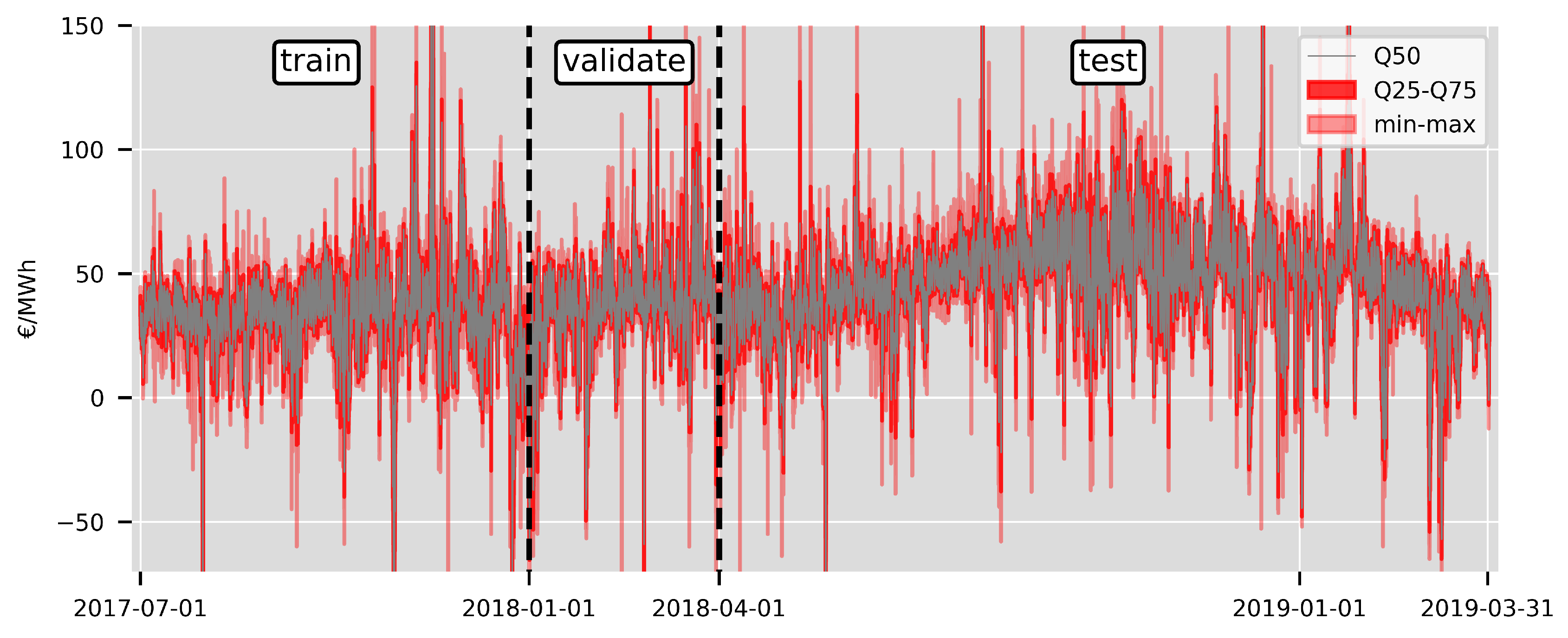
For the empirical forecasting study we consider the entire data set from 1 July 2017 till 31 March 2019 with the initial training, validation, and test split shown in Figure 3. We use the first six months of data from 1 July 2017 till 31 December 2017 as initial training set to forecast the quantiles for all hours of the following day. We then shift the training set by one day, refit all models, and again forecast the following day. We use the first three months of 2018 as a validation set to fix the values for considering values on an exponential grid given by . The value of for each is determined by the lowest mean absolute error. The 12 months between April 2018 and March 2019 form the test set. In cases where there was no trading between two time steps for a product, we reuse the quantile values from the preceding 15 min time interval. If there was no trading in any preceding periods, we set all quantile values to the day-ahead auction price. To account for the numerical instability of the neural network’s predictions resulting from the random weight initialization and the non-convex loss function, we train an ensemble of 5 models and average their predictions.
4.2. Evaluation
We use two measures to evaluate the accuracy of the predictions for the entire distribution, the Wasserstein distance (WD) and integrated quadratic distance (QD). These distances provide an intuitive way to measure the difference between two empirical distributions in a non-parametric way. For two univariate distributions P and S with cumulative density functions (CDF) F and G the WD is defined as and the QD is defined as . Hence, we compute the errors by
and
respectively, where is described by the predicted vector of quantile values and is the true VWECDF.
To measure the overall the forecast accuracy we compute the mean Wasserstein distance (MWD)
and mean integrated quadratic distance (MQD)
where D is the number of days in the test set.
To investigate the difference in forecasting accuracy for different quantiles we compute the mean absolute error (MAE) and root mean squared error (RMSE) values for each quantile separately
Since the values of the error measures alone do not allow for a statistically sound conclusion on the outperformance of forecast A by forecast B, we employ the Diebold-Mariano (DM) test [21] in the modified version proposed by Harvey et al. [22] as implemented in the R forecast package [23]. The DM test examines the statistical significance of the difference of the residual time series of two models. We compute the multivariate version of the test as proposed in [24], i.e., we obtain one error for each day by computing a norm for the vector of residuals for the day d.
We consider two variants of the test as we expect a difference in forecasting ability for different quantiles. In the first variant we compute the L1 norm of the WDs and the L2 norm of the QDs over one day
Then the loss differential for two forecasts A and B is given by and , respectively. For both error measures and all model combinations we conduct a pair of two one-sided DM tests and report the p-values for the hypothesis and , respectively.
In the second variant we compare the and norms of the errors for only a single quantile , i.e., we compute
with and obtain one loss differential per quantile . We again conduct a pair of two one-sided DM tests for both measures for the loss differential of the quantile forecasts, i.e., we report the p-values for the hypothesis and for all models and all quantiles.
5. Results
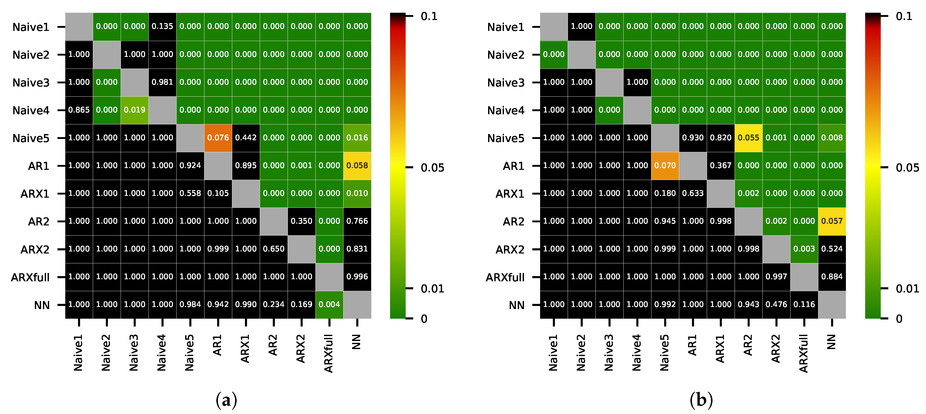
We present the MWD and MQD values in Table 1 and the corresponding DM test p-values in Figure 4a,b. All statistical models except AR1 show lower MWD and MQD values than the best benchmark model Naive5. The differences in accuracy between the forecasts of AR1, ARX1, and Naive5 are not significant. The forecasts of the ARXfull model give the best results in terms of both measures. The improvements of the ARXfull forecasts in terms of MWD and MQD compared to the best benchmark model Naive5 are only about 2% and 3.5%. In terms of MWD, the improvement in accuracy of the ARXfull forecasts is significant compared to all models. Considering MQD, the improvement in accuracy of the ARXfull forecasts is significant compared to all models except the NN. There is no statistical significant difference in the accuracy of the forecasts from the AR2, ARX2, and NN models. Furthermore, we can not report a significant difference in accuracy between the forecasts from AR1 and ARX1 as well as between the forecasts from AR2 and ARX2.
These observations lead to several conclusions. Incorporating exogenous variables does not improve the forecasting performance while considering time series information from the neighboring products leads to a significant improvement. Furthermore, the inclusion of information from other quantiles in combination with automated variable selection using Lasso also improves the forecasting performance significantly.
Table 2 and Table 3 present the values for and for selected quantiles. This allows a more detailed analysis regarding the forecasting accuracy for different regions of the distribution. The forecasts from the ARXfull model show the lowest values for all quantiles except Q90 and Q100. For these quantiles the NN forecasts are more accurate. The NN forecasts show larger errors for the central quantiles than the predictions of the much simpler AR2 and ARX2 models. However, the accuracy of the NN forecasts is better for the more extreme quantiles. This could be explained by non-linear effects that can not be modeled by the linear regression approach. The findings are similar for the RMSE. The ARXfull model shows the best performance for the central quantiles while the NN model shows slightly better performance for the tails. In general, errors are larger for the tails of the distribution across all models, especially for the minimum and maximum values.
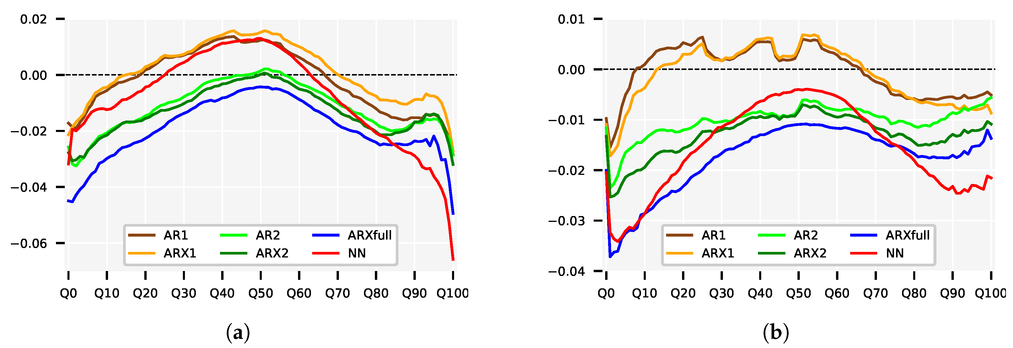
Figure 5a,b show the relative improvement in and for the statistical models compared to the forecasts of the best performing benchmark model Naive5. In terms of only the ARXfull forecasts show a small relative improvement for the central quantiles of roughly . The relative gains in accuracy are larger for the tails for all models, e.g., the ARXfull forecasts show a relative improvement of respectively and for Q10 and Q90.
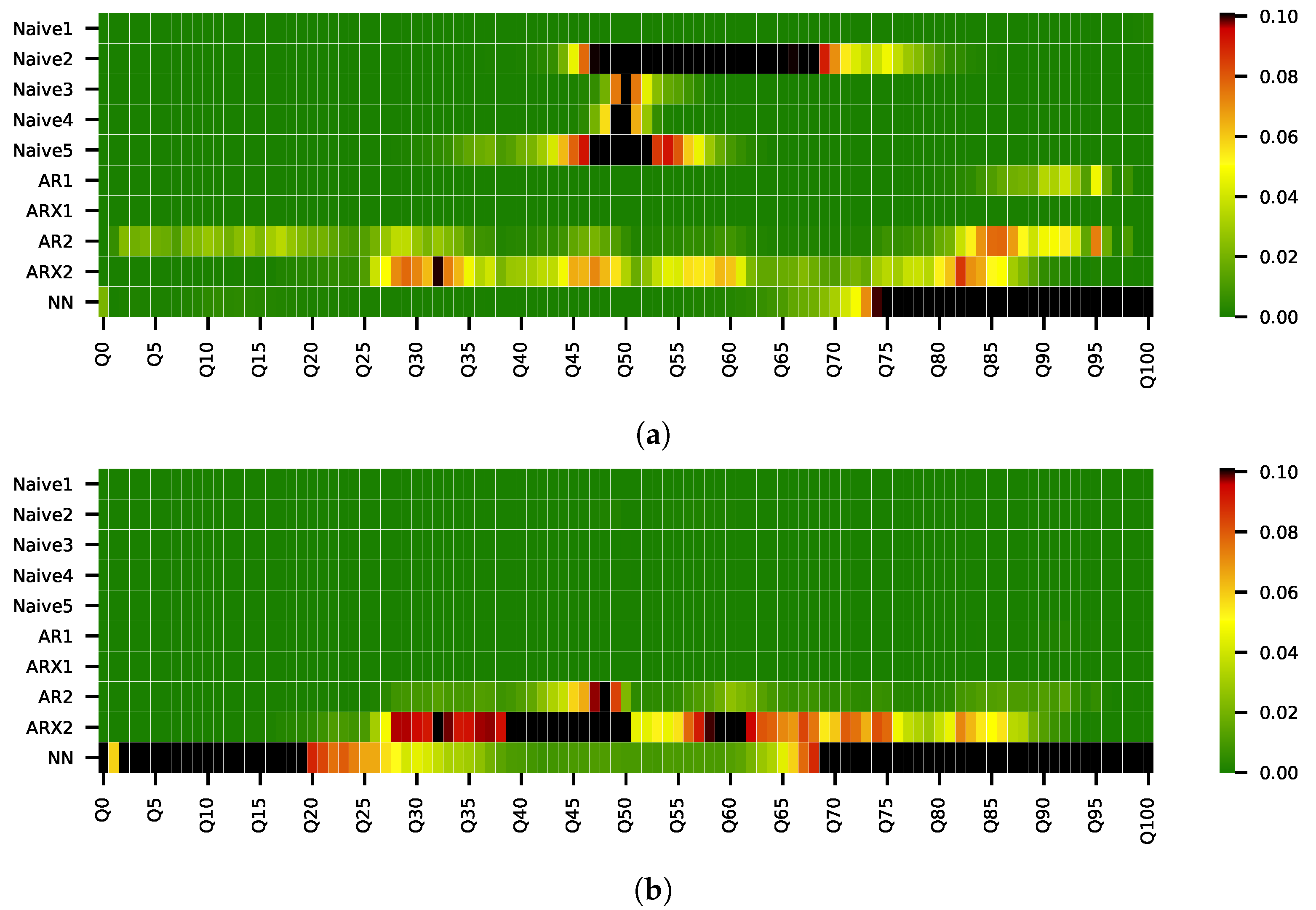
Figure 6a,b show the p-values of the DM-test for the loss differential per quantile for the ARXfull forecasts against all other models’ forecasts for the L1 and L2 norm, respectively. As can be seen from Figure 6a, we can not conclude a significantly improved forecasting accuracy in comparison to the forecasts of Naive2 to Naive5 in terms of MAE for the central quantiles. However, the accuracy is significantly better for the tails of the distribution. Considering the RMSE, the improvement over the benchmarks is significant for all quantiles. These results suggest that it is possible to forecast the short-term volatility of the intraday market which is reflected in the tails of the volume-weighted price distribution. At the same time, we can not report a definite improvement over the naive models for the central quantiles considering the inconsistent results for MAE and RMSE.
6. Conclusions
We analyzed the German continuous intraday electricity market and focused on hour products and the last three hours before delivery. We proposed to non-parametrically approximate the empirical volume-weighted price distribution by using a dense grid of discrete quantiles. This admits a much richer representation of the market behavior than only analyzing volume-weighted average prices. In order to forecast the quantile values of this distribution we constructed a set of simple linear regression models that use different subsets of the available inputs. Furthermore, we used two more advanced models that utilize all available regressors, a Lasso regularized linear regression model and an ensemble of multi-output neural networks. We found that including exogenous variables did not improve the accuracy while considering time series information from neighboring products and quantiles did. We compared the forecasts of the proposed models with several simple but well designed benchmarks. The best performing model turned out to be the Lasso regularized linear regression model. We also studied the forecasting accuracy for different quantiles of the price distribution. Compared to the naive benchmarks, the gains in forecasting performance were small and not significant for the central quantiles of the target distribution. However, the gains in accuracy for the tails of the distributions were larger and significant. Hence, we gather evidence that the German intraday market works efficiently while also showing that it is possible to forecast the variance of short-term intraday prices.
There are several avenues for future work. It would be interesting to see if we would obtain similar findings for quarter hour products which we excluded in this work. It is also worth investigating if information from quarter-hour products could help to improve the forecast accuracy for the hour products and vice versa. We chose to model the price distribution in a non-parametric way which allows a larger degree of flexibility. However, modeling the price distribution in a parametric way is straightforward and worth exploring. Furthermore, we solely focused on prices while an estimate of the expected traded volume as a measure of short-term market liquidity would also be of interest in practice. Finally, future work should explore how to exploit forecasts for the distribution of prices and volumes for short-term trading and risk management.
Author Contributions
Conceptualization, T.J. and F.S.; methodology, T.J.; software, T.J.; validation, T.J.; formal analysis, T.J.; investigation, T.J.; data curation, T.J.; writing—original draft preparation, T.J.; writing—review and editing, T.J. and F.S.; visualization, T.J.; supervision, F.S.
Funding
This research was partially funded by the TU Darmstadt Pioneer Fund.
Conflicts of Interest
The authors declare no conflict of interest.
Abbreviations
The following abbreviations are used in this manuscript:
| CDF | cumulative density function |
| DM | Diebold-Mariano |
| MAE | mean absolute error |
| MQD | mean integrated quadratic distance |
| MWD | mean Wasserstein distance |
| QD | integrated quadratic distance |
| RMSE | root mean squared error |
| VWECDF | volume-weighted empirical cumulative density function |
| WD | Wasserstein distance |
References
- Ocker, F.; Ehrhart, K.M. The “German Paradox” in the balancing power markets. Renew. Sustain. Energy Rev. 2017, 67, 892–898. [Google Scholar] [CrossRef]
- Koch, C.; Hirth, L. Short-term electricity trading for system balancing: An empirical analysis of the role of intraday trading in balancing Germany’s electricity system. Renew. Sustain. Energy Rev. 2019, 113, 109–275. [Google Scholar] [CrossRef]
- EPEXSpot. Traded Volumes Soar to an All Time High in 2018. 2018. Available online: https://www.epexspot.com/en/press-media/press/details/press/Traded_volumes_soar_to_an_all-time_high_in_2018 (accessed on 4 November 2019).
- EPEXSpot. Description of Epex Spot Market Indices (May 2019). 2019. Available online: https://www.epexspot.com/document/39669/EPEX%20SPOT%20Indices (accessed on 4 November 2019).
- Viehmann, J. State of the German Short-Term Power Market. Z. Für Energiewirtschaft 2017, 41, 87–103. [Google Scholar] [CrossRef]
- Weron, R. Electricity price forecasting: A review of the state-of-the-art with a look into the future. Int. J. Forecast. 2014, 30, 1030–1081. [Google Scholar] [CrossRef] [Green Version]
- Andrade, J.; Filipe, J.; Reis, M.; Bessa, R. Probabilistic price forecasting for day-ahead and intraday markets: Beyond the statistical model. Sustainability 2017, 9, 1990. [Google Scholar] [CrossRef]
- Monteiro, C.; Ramirez-Rosado, I.; Fernandez-Jimenez, L.; Conde, P. Short-term price forecasting models based on artificial neural networks for intraday sessions in the iberian electricity market. Energies 2016, 9, 721. [Google Scholar] [CrossRef]
- Maciejowska, K.; Nitka, W.; Weron, T. Day-Ahead vs. Intraday—Forecasting the Price Spread to Maximize Economic Benefits. Energies 2019, 12, 631. [Google Scholar] [CrossRef]
- Uniejewski, B.; Marcjasz, G.; Weron, R. Understanding intraday electricity markets: Variable selection and very short-term price forecasting using LASSO. Int. J. Forecast. 2019, 35, 1533–1547. [Google Scholar] [CrossRef] [Green Version]
- Narajewski, M.; Ziel, F. Econometric modelling and forecasting of intraday electricity prices. arXiv 2018, arXiv:1812.09081. [Google Scholar] [CrossRef]
- EPEXSpot. Available online: www.epexspot.com (accessed on 4 November 2019).
- ENTSOE-E. transparency Platform. Available online: transparency.entsoe.eu (accessed on 4 November 2019).
- EPEXSpot. Epex Spot Market Rules. 2019. Available online: http://www.epexspot.com/de/extras/download-center (accessed on 4 November 2019).
- Tibshirani, R. Regression shrinkage and selection via the lasso. J. R. Stat. Soc. Ser. B (Methodol.) 1996, 58, 267–288. [Google Scholar] [CrossRef]
- Clevert, D.A.; Unterthiner, T.; Hochreiter, S. Fast and Accurate Deep Network Learning by Exponential Linear Units (ELUs). arXiv 2015, arXiv:1511.07289. [Google Scholar]
- Kingma, D.P.; Ba, J. Adam: A Method for Stochastic Optimization. arXiv 2014, arXiv:1412.6980. [Google Scholar]
- Chollet, F. Keras. 2015. Available online: https://keras.io (accessed on 4 November 2019).
- Uniejewski, B.; Weron, R.; Ziel, F. Variance Stabilizing Transformations for Electricity Spot Price Forecasting. IEEE Trans. Power Syst. 2018, 33, 2219–2229. [Google Scholar] [CrossRef]
- Huber, P.J. Robust Estimation of a Location Parameter. Ann. Math. Statist. 1964, 35, 73–101. [Google Scholar] [CrossRef]
- Diebold, F.; Mariano, R. Comparing Predictive Accuracy. J. Bus. Econ. Stat. 1995, 13, 253–263. [Google Scholar] [Green Version]
- Harvey, D.; Leybourne, S.; Newbold, P. Testing the equality of prediction mean squared errors. Int. J. Forecast. 1997, 13, 281–291. [Google Scholar] [CrossRef]
- Hyndman, R.J.; Khandakar, Y. Automatic time series forecasting: The forecast package for R. J. Stat. Softw. 2008, 26, 1–22. [Google Scholar]
- Ziel, F.; Weron, R. Day-ahead electricity price forecasting with high-dimensional structures: Univariate vs. multivariate modeling frameworks. Energy Econ. 2018, 70, 396–420. [Google Scholar] [CrossRef] [Green Version]
Figure 1.
(a) The figure shows all trades that were executed from 5 to 0 h before delivery for the hour product on 10.8.2018 in gray circles. Circles are scaled according to trade volume. The shaded red regions show values for selected quantiles in the 15 min time intervals. (b) The red function is the inverse of the volume-weighted empirical cumulative distribution function for the last 5 h of trading. The black markers depict selected quantiles, e.g., the black square represents .

Figure 2.
Visualization of the neural network model. The first layer is a locally connected layer that operates only on the time series data and learns a distinct set of weights per quantile. The layer’s output is concatenated with the vector of exogenous variables and passed through a fully connected layer.

Figure 3.
Selected quantiles of the intraday price distribution from 3 h to 0.5 h before delivery for the entire data set. The initial training set contains six months of data from June 2017 to December 2017. The first three months of 2018 are used to fix the hyperparameters for the elastic net models. The test set contains 12 months of data from April 2018 to March 2019. We refit all models each day using a rolling window scheme.

Figure 4.
p-values of the multivariate DM test for (a) daily the L1 norm of the WD and (b) the daily L2 norm of the QD. p-values close to zero (dark green) indicate that the forecasts from the model on the x-axis are significantly more accurate than the forecasts from the model on the y-axis.
Figure 4.
p-values of the multivariate DM test for (a) daily the L1 norm of the WD and (b) the daily L2 norm of the QD. p-values close to zero (dark green) indicate that the forecasts from the model on the x-axis are significantly more accurate than the forecasts from the model on the y-axis.

Figure 5.
Relative difference in (a) MAE and (b) RMSE values per quantile of the statistical models compared to Naive5. Values smaller than zero indicate smaller errors than Naive5.
Figure 5.
Relative difference in (a) MAE and (b) RMSE values per quantile of the statistical models compared to Naive5. Values smaller than zero indicate smaller errors than Naive5.

Figure 6.
The figure shows the p-values for the multivariate DM tests per quantile for (a) the daily L1 norm and (b) the daily L2 norm for the forecasts of the ARXfull model compared against the forecasts of all other models. Dark green cells indicate that the forecasts of the ARXfull model are significantly more accurate than the forecasts from the model on the y-axis for the quantile given on the x-axis.


Table 1.
MWD and MQD values for the test set in .
| Naive1 | Naive2 | Naive3 | Naive4 | Naive5 | AR1 | ARX1 | AR2 | ARX2 | ARXfull | NN | |
|---|---|---|---|---|---|---|---|---|---|---|---|
| MWD | 4.147 | 3.912 | 4.008 | 4.091 | 3.803 | 3.789 | 3.801 | 3.751 | 3.747 | 3.721 | 3.763 |
| MQD | 1.938 | 2.041 | 1.535 | 1.585 | 1.414 | 1.418 | 1.409 | 1.395 | 1.375 | 1.362 | 1.371 |
Table 2.
Test set mean MAE values for selected quantiles in .
| Naive1 | Naive2 | Naive3 | Naive4 | Naive5 | AR1 | ARX1 | AR2 | ARX2 | ARXfull | NN | |
|---|---|---|---|---|---|---|---|---|---|---|---|
| Q0 | 7.52 | 8.96 | 8.23 | 8.45 | 7.11 | 6.99 | 6.96 | 6.93 | 6.91 | 6.79 | 6.88 |
| Q10 | 4.62 | 4.61 | 4.65 | 4.70 | 4.23 | 4.21 | 4.21 | 4.15 | 4.14 | 4.11 | 4.18 |
| Q20 | 4.10 | 3.85 | 3.97 | 4.00 | 3.71 | 3.71 | 3.72 | 3.65 | 3.65 | 3.62 | 3.69 |
| Q30 | 3.80 | 3.43 | 3.52 | 3.53 | 3.38 | 3.40 | 3.40 | 3.35 | 3.34 | 3.33 | 3.39 |
| Q40 | 3.70 | 3.26 | 3.30 | 3.31 | 3.24 | 3.28 | 3.29 | 3.24 | 3.23 | 3.21 | 3.28 |
| Q50 | 3.68 | 3.21 | 3.21 | 3.21 | 3.21 | 3.25 | 3.25 | 3.21 | 3.21 | 3.19 | 3.25 |
| Q60 | 3.69 | 3.22 | 3.27 | 3.30 | 3.24 | 3.26 | 3.27 | 3.23 | 3.22 | 3.21 | 3.25 |
| Q70 | 3.75 | 3.34 | 3.45 | 3.55 | 3.37 | 3.35 | 3.37 | 3.33 | 3.33 | 3.31 | 3.34 |
| Q80 | 3.99 | 3.69 | 3.88 | 4.02 | 3.70 | 3.65 | 3.67 | 3.63 | 3.62 | 3.61 | 3.62 |
| Q90 | 4.50 | 4.43 | 4.60 | 4.82 | 4.31 | 4.24 | 4.27 | 4.24 | 4.24 | 4.21 | 4.18 |
| Q100 | 7.38 | 8.49 | 8.18 | 8.66 | 7.36 | 7.16 | 7.16 | 7.15 | 7.13 | 7.00 | 6.88 |
Table 3.
Test set mean RMSE values for selected quantiles in .
| Naive1 | Naive2 | Naive3 | Naive4 | Naive5 | AR1 | ARX1 | AR2 | ARX2 | ARXfull | NN | |
|---|---|---|---|---|---|---|---|---|---|---|---|
| Q0 | 14.19 | 15.64 | 17.01 | 17.10 | 13.07 | 12.95 | 12.93 | 12.92 | 12.90 | 12.81 | 12.80 |
| Q10 | 7.10 | 7.20 | 6.88 | 7.05 | 6.22 | 6.23 | 6.20 | 6.14 | 6.10 | 6.04 | 6.04 |
| Q20 | 6.30 | 6.05 | 5.95 | 6.03 | 5.54 | 5.57 | 5.56 | 5.48 | 5.46 | 5.42 | 5.44 |
| Q30 | 5.88 | 5.36 | 5.36 | 5.41 | 5.17 | 5.17 | 5.17 | 5.11 | 5.10 | 5.08 | 5.11 |
| Q40 | 5.77 | 5.10 | 5.09 | 5.12 | 5.03 | 5.06 | 5.06 | 4.99 | 4.99 | 4.97 | 5.00 |
| Q50 | 5.79 | 5.04 | 5.04 | 5.04 | 5.04 | 5.06 | 5.06 | 5.00 | 5.00 | 4.98 | 5.02 |
| Q60 | 5.88 | 5.15 | 5.19 | 5.21 | 5.13 | 5.15 | 5.15 | 5.09 | 5.08 | 5.07 | 5.10 |
| Q70 | 6.19 | 5.60 | 5.82 | 5.88 | 5.51 | 5.50 | 5.50 | 5.46 | 5.45 | 5.43 | 5.44 |
| Q80 | 6.88 | 6.56 | 6.91 | 7.09 | 6.27 | 6.23 | 6.23 | 6.20 | 6.18 | 6.16 | 6.15 |
| Q90 | 8.53 | 8.60 | 9.21 | 9.58 | 7.98 | 7.93 | 7.92 | 7.91 | 7.87 | 7.84 | 7.79 |
| Q100 | 19.73 | 20.41 | 24.68 | 25.38 | 18.81 | 18.72 | 18.65 | 18.71 | 18.61 | 18.56 | 18.41 |
© 2019 by the authors. Licensee MDPI, Basel, Switzerland. This article is an open access article distributed under the terms and conditions of the Creative Commons Attribution (CC BY) license (http://creativecommons.org/licenses/by/4.0/).
Share and Cite
MDPI and ACS Style
Janke, T.; Steinke, F. Forecasting the Price Distribution of Continuous Intraday Electricity Trading. Energies 2019, 12, 4262. https://0-doi-org.brum.beds.ac.uk/10.3390/en12224262
AMA Style
Janke T, Steinke F. Forecasting the Price Distribution of Continuous Intraday Electricity Trading. Energies. 2019; 12(22):4262. https://0-doi-org.brum.beds.ac.uk/10.3390/en12224262
Chicago/Turabian StyleJanke, Tim, and Florian Steinke. 2019. "Forecasting the Price Distribution of Continuous Intraday Electricity Trading" Energies 12, no. 22: 4262. https://0-doi-org.brum.beds.ac.uk/10.3390/en12224262
Note that from the first issue of 2016, this journal uses article numbers instead of page numbers. See further details here.