Modeling Intraday Markets under the New Advances of the Cross-Border Intraday Project (XBID): Evidence from the German Intraday Market


University of Duisburg-Essen, 45141 Essen, Germany
†
Current address: Altenessenerstr. 27, 45141 Essen, Germany.
Energies 2019, 12(22), 4339; https://0-doi-org.brum.beds.ac.uk/10.3390/en12224339
Submission received: 24 October 2019
/
Revised: 10 November 2019
/
Accepted: 11 November 2019
/
Published: 14 November 2019
(This article belongs to the Special Issue Modeling and Forecasting Intraday Electricity Markets)
Abstract
:The intraday cross-border project (XBID) allows intraday market participants to trade based on a shared order book independent of countries or local energy exchanges. This theoretically leads to an efficient allocation of cross-border capacities and ensures maximum market liquidity across European intraday markets. If this postulation holds, the technical implementation of XBID might mark a regime switch in any intraday price series. We present a regression-based model for intraday markets with a particular focus on the German European Power Exchange (EPEX) intraday market and evaluate if the introduction of XBID influence prices, volume or volatility. We analyze partial volume-weighted average prices and standard deviations as well as cross-border volumes at different trading times. We are able to falsify our initial hypothesis assuming a measurable influence of changes caused by XBID. Thus, this paper contributes to the ongoing discussion on appropriate modeling of intraday markets and demonstrates that XBID does not necessarily need to be included in any model.
1. Introduction
Nowadays, there is a rapid speed of change in short-term electricity market conditions in Europe. In the old days, trading was a local phenomenon with only a few large utilities participating in wholesale trades. Now, facilitated by European guidelines and ongoing liberalization, new opportunities are evolving. Current electricity spot trading is characterized by different time horizons of trading, with a clear tendency towards shorter time horizons and an increasing share of cross-border trading with other European countries. Germany is outstanding in the picture of the virtual pan-European copper plate such that it is very progressive in terms of market development and liquidity.
It is important to understand and model the market structure under such dynamic conditions. In an environment where intraday markets gain more attention, asset-owners and portfolio managers need to make precise decisions. Consequently, there is a growing body of literature that deals with modeling intraday markets and their determinants. The first publications have valued the intraday market as an alternative to other trading venues such as the day-ahead or the balancing market and evaluated optimal bidding behavior. Papers such as Garnier and Madlener [1] or Aïd et al. [2] also mention market liquidity or wind generation as key drivers of intraday trading. Kiesel and Paraschiv [3] expanded the view on 15-min intraday trading. Additional thoughts on fundamental factors driving German intraday prices can be found in Pape et al. [4].
While the latter papers set their focus on determinants and bidding, there is also a growing tendency towards electricity price forecasting of intraday markets. Andrade et al. [5] and Monteiro et al. [6] propose forecasting models for Iberian intraday prices, while Uniejewski et al. [7] try to forecast very short-term prices in German intraday markets. Narajewski and Ziel [8] combined a forecasting study with determinant analysis and elaborated the value of information present in the continuous trading for short-term price forecasts.
Most of the previously mentioned papers solely model as an isolated market using national determinants. On the other hand, current market trends point towards a stronger interaction of countries in intraday electricity markets. We want to analyze the effect of such ongoing market integration in its most current extension, XBID. Section 2 takes a deeper look at market integration. How is Germany connected to other markets and what is the importance of the newly introduced XBID regime in that sense? Based on such, Section 2.3 proposes three simple hypotheses that serve as lines of thought throughout the entire paper. We discuss our choice of intraday data, present other influential factors and customize a regression set-up to the data in Section 3. We present linear-model results in Section 4, their non-linear outcomes in Section 5 and summarize our findings and contribution of this paper in Section 6.
2. Cross-Border Trading in the German Intraday Market under XBID
2.1. Market Integration in European Short-Term Energy Markets
The idea of connecting different electricity spot markets goes back to a time when Germany was not liberalized. Already in 2002, day-ahead capacities were explicitly allocated between Germany and Denmark as reported in Kristiansen [9]. Later in 2006, Belgium, the Netherlands and France were coupled with the German day-ahead market (Oggioni and Smeers [10]). The first one to look at intraday markets was Hagemann [11] who found some evidence for the importance of flows from France to Germany and—in a limited manner—vice versa.
Most of the papers that deal with cross-border trading have a particular focus on policy implications or analytical insights, e.g. the impact of European flows on a national level. Ziel et al. [12] studied the cross-country effects of early day-ahead EXAA prices on its connected day-ahead exchanges with a focus on forecasting. Panapakidis and Dagoumas [13] added some connected European market prices and demonstrated the gains in accuracy if one does not only consider national exogenous variables but also other cross-border prices. A similar idea was realized in Lago et al. [14] and Lago et al. [15] where the authors proposed a forecasting model that incorporates market integration in day-ahead markets through the addition of features stemming from connected countries.
Table 1 focuses on the total scheduled flow between Germany and its neighbors based on official ENTSO-E data of 2018. Unfortunately, explicit data sources for the intraday time frame are rather sparse which is why we take into account the total commercial exchanges. They comprise all information starting from long-term capacities over day-ahead ones to intraday without any separation into implicit or explicit allocation. One might argue that this is not intraday data per se, but taking into consideration the entire amount of utilized capacities ensures a global view that captures the importance of this time series. Besides, dedicated intraday data is not available in all cases.
The most important counterpart for Germany in terms of cross-border trading is Austria. Please note that the terminology of this paper is strictly limited to applications in electricity intraday trading. Terms like ‘cross-border’ or ‘trade’ may be associated with the field of foreign trade or general economics. However, this paper solely deals with electricity trading topics. If we recall that Germany and Austria were considered as one bidding zone until October 2018 this comes as no surprise. France and the Netherlands follow, with more than half of the Austrian volume. In all three cases, Germany is a net exporter of electricity to those regions. This is different from the Czech Republic. Germany imports more than it exports over the Czech border.
Of course, flows alone are only one side of the coin. Equally important are the means of allocating capacities. There are two basic ways to allocate them among market participants: Explicit allocation, usually done in a pay as bid manner, and implicit allocations based on market prices. The second alternative theoretically leads to more global benefits in the form of lower market prices for all actors without any risk of market manipulation by single participants. Thoughts on the efficiency of the early market integration can be found in Zachmann [16]. Figure 1 summarizes how intraday allocation was done before and how it is done after the introduction of XBID. The depiction is not limited to Germany which allows us to derive all participating XBID member states. If we draw our attention to the Nordic region it is evident that it was already implicitly coupled before XBID. The same counts for the western European capacities between Germany, the Netherlands, Belgium, and France. Yet, there is one exception: A special case is the French-German border with two available allocation mechanisms. One can use explicit allocations but in case of insufficient demand, the implicit XBID allocation is also possible. More information on that special case is provided by the grid operators in Amprion GmbH [17]. Eastern European countries like Poland or the Czech Republic are as yet only coupled explicitly but are planned to be part of a second implementation wave in late-2019.
Another crucial aspect to mention is the coverage of market integration. If there is sufficient capacity, it is possible that trading occurs between Spain and Norway, for instance. While before XBID such a cross-border trade was connected to several operational burdens like bidding at various exchanges and different capacity nominations systems, under XBID it is possible that a deal happens with a simple click in the order book of one of the participating exchanges. We want to conclude our view on European market integration with a short look into the future. European TSOs (transmission service operators) are currently determining a way to implement the new guidelines on bidding zones and their connected calculation of cross-border capacities. Based on European government plans, they are obliged to increase the level of capacities used for market coupling and reduce the partition currently used for grid security reasons. More information can be found in the official report in ENTSO-E [19].
2.2. XBID as a Particular Enhancement of Market Integration
The previous sub-chapter briefly discussed XBID under the aspect of market integration in general. The Cross-Border Intraday Project (XBID), that went live on delivery date 18 June 2018, was brought forward by a consortium of four energy exchanges and 17 TSOs based on an EU Commission legislation postulated in Commission [20]. It demands a joint and efficient allocation of intraday capacities and easy access to a singular European market knowing full well that this is contrary to the individual business interests of singular exchanges. One key component is the shared order book for European intraday markets. An IT system hosted by Deutsche Börse AG provides the infrastructure to a singular order book that aggregates orders from the participating exchanges: EPEX Spot SE, Nord Pool, GME in Italy and the Spanish exchange OMIE (EPEX Spot SE [18]). The shared order book is accompanied by a capacity management module and a shipping module responsible for managing capacity allocation and nomination.
But how does this work in practice? Figure 2 depicts the basic principle based on a simple toy example. Suppose we have only two participating countries, Germany and Denmark. First of all, the two relevant TSOs will jointly determine the volume of available transfer capacities for XBID and release those to the XBID system. The volume itself depends on technical available capacities, day-ahead or long-term capacity volume contracts and reserves for reasons of grid security. In our concrete case, 50 MW could be transferred in one hour from Denmark to Germany. With such information, the XBID system can now start to couple national order books to utilize the 50 MW for welfare maximization. The example shows how both the Danish and the German trader enter a sell and buy order at 50 EUR/MWh. Without coupling, the Danish sell order would remain within the local order book such that no deal is done. But under consideration of the available capacity, the willingness to buy and sell can be matched across the border and a trade is done at 50 EUR/MWh. On a national level, we also have aggregated orders from various exchanges such that the order submitted to the EPEX and Nord Pool intraday system is considered singularly. If—and only if—there is sufficient capacity, order books are coupled with neighboring countries.
One aspect has deliberately been ignored in the toy example. Of course, an interaction between several TSOs has to follow a certain protocol. XBID alignments are carried out under the timelines displayed in Figure 3. German intraday trading starts around 15:00 day-ahead in local markets without any market coupling at all. Parties can already nominate their trades but the first actual TSO matching happens at 18:00 day-ahead. Capacities to northern European countries such as Denmark are available at the same time so that the XBID-coupled trading starts at 18:00 day-ahead. During the night, at 22:00 day-ahead, the rest of the European capacities are made available to the XBID system. After that, the markets are—given sufficient capacity—fully coupled until 60 min before delivery. While the order book is cleared of all XBID orders by then, the German intraday trading continues in its known local form afterward.
2.3. Connected Research Hypotheses and Associated Empirical Framework
Based on the above information on XBID and market integration of intraday markets, we propose three simple, descriptive hypotheses. They serve as a formal structure and a summarizing element for the academic insights that this paper contributes. Following the idea of Popper [21], we can falsify or accept hypotheses. Please note that we will firstly present a descriptive, non-mathematical formulation of our research hypotheses H1, H2, and H3. They shall give the reader an impression of what we will test in subsequent chapters and they will also be referred to in the concluding Section 6. Besides the intuitive hypotheses, we will shortly discuss the empirical framework that goes along with H1, H2 and H3. We define certain criteria for acceptance and describe the statistical hypotheses and decision criteria associated with H1, H2, and H3. Please note that the empirical test set-up does not change for any of the research hypotheses, meaning that H1, H2, and H3 are all evaluated based on the same statistical metrics. The only thing that differs is the object of analysis, since H1 deals with intraday prices, H2 with volume and H3 with volatility expressed as standard deviation. In detail, we want to test the following:
Hypothesis 1 (H1).
XBID influences intraday prices /. If markets are coupled more appropriately, this could lead to fewer inefficiencies as reported in Zachmann [16]. Hence, XBID might potentially lower price levels through less efficient usage of capacities.
Hypothesis 2 (H2).
XBID affects cross-border. volumes . A more efficient usage of capacities could lead to higher trading volume which is a prerequisite for an efficient market according to Hagemann and Weber [22] and Weber [23]. Since XBID directly affects the allocation of capacities and adds different European orders to local order books, it may increase trading volume and market efficiency.
Hypothesis 3 (H3).
The introduction of XBID drives intraday price volatility . Price volatility or large spikes between different countries might be a sign of inefficiency according to Zachmann [16]. On the other hand, Weber [23] points out that fewer arbitrage opportunities in intraday trading render the market more efficient. Based on such thoughts, XBID could potentially lower volatility due to its increased amount of orders stemming from other countries and, therefore, have a positive impact on market efficiency.
More formally, H1, H2, and H3 are confirmed if two statistical acceptance criteria are met. A graphical representation of the twofold test logic is given in Figure 4. The first empirical test is constructed using a linear regression as described in Section 3.6 and Section 3.7. One part of H1, H2 and H3 is confirmed if we can reject the null hypothesis that of Equations (6) and (7) in case of intraday price spreads, intraday cross-border volumes and the standard deviation of prices. Hence, we assess H1, H2, and H3 based on the statistical significance of the XBID coefficient in a linear regression model. We construct two regressions (see Equations (6) and (7) for details) for more robust findings. However, since Equation (7) is the one comprising all the variables, we give the results of this regression more weight and only use Equation (6) as a means to verify the adequacy of our results.
But that is only the first acceptance criterion. The above-mentioned procedure only checks for significance in a linear set-up and implies the drawbacks of a linear model. Therefore, a random forest model using , and as predictors and data of Equations (6) and (7) as explanatory variables yield a variable important measure as output. This measure is the increase in MSE (denoted as %INC(MSE)) assuming that we randomly change values of one input variable while keeping all other regressors of Equations (6) and (7) equal. Research hypotheses H1, H2 and H3 are confirmed if , meaning that %INC(MSE) accounts for a large portion of the most informative variable, i.e., the XBID dummy variable has a high relative importance in the non-linear model. More information on the random forest approach is provided in Section 5. Both empirical tests need to suggest the same outcome for acceptance of H1, H2, and H3.
3. Data and Aggregation Methodology
3.1. The Necessity to Aggregate Deal Information in Intraday Markets
The intraday market is a pay-as-bid market meaning that a deal is done if the exchange can match two orders at an identical price. This matching procedure results in thousands of transactions with different volumes and prices. Average prices are already available in an aggregated time series but XBID stops one hour before delivery which renders the usual price indices reported by EPEX Spot impractical. We have to exclude the periods where no XBID trades are observed. This ensures that there is no undesired influence of strong local, non-cross-border trading implications. Therefore, this paper focuses on partial average prices tailor-made to reflect cross-border trading. Firstly, it is important to note the notational difference between delivery-hour and its connected trading times. Often also referred to as ‘product’, the delivery-hour describes the respective time in which the physical delivery takes place. Hence, ‘hour 20’ as delivery hour or product describes physical delivery from 19:00 until 20:00 and is tradable many hours before. This time-span, the trading time, is very important understanding the methodology.
We denote the end of a trading time for a specific product as . Instead of using published indices, we pivot for a specific time range. The notation describes a set of time-stamps and their connected transactions that are part of the overall set of public trades. Transactions must be element of the time frame with or are excluded. The index i can also be seen as the hours before delivery. A public EPEX transaction for any specific delivery hour consists of a price , its volume , a buying and a selling country (jointly denoted as C) and a time stamp. We aggregate the time stamp as follows: The time-stamps will be part of which is why the index i is sufficient to explain the hourly time horizon. A more concrete example helps in fully grasping the idea. Take volume-weighted prices for instance, then (based on Narajewski and Ziel [8])
where describes the time-weighted average price for time stamp range i and country C with volume being the volume of each n-th public transaction and its connected trade price. In other words, this means that is the volume-weighted average price spanning all Dutch transactions in a period from 2 h up to 60 min before delivery. This study applies a horizon of . We deliberately chose to compute each hourly time frame separately as we might get additional insight from the hourly separation. Computing the analysis over the entire time horizon, i.e., a time between 2 up to 4 h before delivery does not change the main message, which is why we have decided to focus on the lower granularity. One could also carry out the analysis for a later time horizon (for instance ). However, that is critical as even the German market is lacking liquidity in very early trading phases. Other more illiquid markets such as Belgium may not even feature any trades, so results get unreliable. Note that this was a first introduction of the underlying filtering concept exemplarily applied on prices. More details follow in the subsequent sections.
3.2. Data: Applied Intraday Prices
In order to analyze price effects, this paper introduces two different kinds of intraday price spread, i.e., differences between individual price series. Section 3.1 also dealt with intraday prices. However, it is important to understand the difference. Section 3.1 introduced the individual intraday prices per country that serve as a basis for Section 3.2 in which we introduce price spreads, i.e., differences of two price series. This paper solely analyzes price spreads as shown in Section 3.2, the earlier definition was just an introduction to the topic. In general, these underlying individual prices are published by the relevant exchange EPEX SPOT SE and are the result of matching buy and sell orders on the intraday trading platform. They are reported in EUR per MWh. The first applied price difference is the commonly used spread between day-ahead prices and intraday prices. As a second object, we focus on cross-border intraday spreads, i.e., the price difference between two countries. We define the price spread per day t and hour h as ) in which C reflects France, Belgium, the Netherlands or the German EPEX day-ahead price of each hour and day. Please note that we deliberately treat the day-ahead price as an individual country to make the notations consistent. Taking differences between intraday TWAPs of Equation (1) of several countries reduces trend components to a minimum and renders the time series more stable. A similar procedure is frequently used in financial applications by calculating returns or log returns. Please note that the TWAP definition of Equation (1) only comprises German intraday transactions (for details on the country filtering please refer to Table 2). Since the bidding zone split between Germany and Austria happened in 2018, we have decided to solely focus on German prices. Other authors such as Pape et al. [4] use the volume-weighted average price (VWAP) as a proxy for continuous intraday trading, but the TWAP framework allows for greater detail. Please note that in some periods there are no reported intraday trades, e.g. in situations of downtimes of the trading platform. Such missing data impedes the calculation of TWAPs which is why we simply use the hourly day-ahead price of the respective country, assuming that this is the last known market price.
Day-ahead/intraday spreads are a common first approximation in the analysis of intraday price behavior. However, this modus operandi has one large drawback in the context of XBID. It narrows the consideration down to a national view. But it might as well be that there is no influence on the German day-ahead/intraday price spread because there are fewer foreign trades involved in this pricing definition. The German TWAPs comprise a minimum of one side to happen in the German grid, i.e., either the sell or the buy-side is required to be German.
However, most of the trades will be double-sided German ones such that no XBID or foreign flows are concerned. That is why we expand the view to cross-border intraday spreads. The choice of countries is justified by the large liquidity of our selected countries in comparison to other intraday markets and our data source, EPEX. Nordic intraday markets are less liquid and only available with Nord Pool subscriptions or reported as an aggregate called ‘XBID’ transactions by EPEX, meaning that there is no clear separation possible. In detail, ’XBID’ transactions mentioned in the EPEX data source comprise any deal done with a foreign exchange such as Nord Pool with EPEX being the other side of the transaction. Since Nord Pool also offers access to the German intraday market, one can hardly derive the actual country with such data.
Table 3 summarizes the statistical properties of the price spread series. If one takes France for example, the minimum spread is below −800 EUR/MWh. This almost seems implausible but indeed there were singular days in 2018 with day-ahead and intraday prices above 800 Euros per MWh. All time series averages are negative and—in the case of Belgium and France—the time series are characterized by high standard deviations. Figure 5 plots the time series in a graphical manner. It highlights the price spread per delivery date and separates the time horizons into XBID and pre-XBID. Overall, the XBID section in red does not seem to be fundamentally different. One could identify—if any at all—a very small increase in volatility and spikes. In case of the German-Belgium spread , this is more easily observable than with the other plots. Yet, this is only a very first conclusion drawn from a plot and requires statistical proof in the later sections.
Dealing with electricity price series also implies seasonality. People, as well as the industry, usually demand less electricity during night hours which causes prices and traded volumes to be higher during the day. The same partially counts for weekends when there is less workforce in operation. Figure 6 analyzes these underlying patterns. Part (a) and (b) plot the weekly and hourly effects on the partial intraday average price and the traded volume based on averaged values. Please note that we are using Germany and the time-stamp range as an example, but the pattern evolves in other countries and for other time-stamp ranges in a similar fashion. Part (a) reflects that prices and traded volumes are lower during night hours. At the same time, prices around hour 8 and 20 are the highest per day. An explanation for this is the shift from base to peak products and the connected ramp up or ramp down procedure of power plants. Before trading hourly, one can trade blocks of hours denoted as ‘base’ or ’baseload’ for all 24 h and ‘peak’ for hours 8 to 20. The shift between those two is usually critical and causes higher prices. A weekly pattern is depicted in section (b). German intraday prices and their associated volatility are lower on the weekend compared with weekdays.
The patterns of intraday prices and volumes are intuitive. But do they translate to spreads and volatility? We analyze the price spread and the volatility of German intraday prices as an example. The volatility in plot (c) appears to be more stable while spreads are higher during night hours and in the afternoon. Interestingly, the volatility seems to be a bit lower during weekend times, as shown in plot (d). The price spread between French and German intraday prices is more stable. To conclude, intraday time series feature hourly and weekly patterns that are strongly present in volume and intraday prices but are less influential in derived time series like standard deviation of prices or price spreads between countries. However, it is essential to account for these patterns in the modeling framework. We will present a possible solution in Section 3.7.
3.3. Data: Aggregated Cross-Border Volumes
One of the major political goals of XBID is the increase of European intraday liquidity. Hence, it is mandatory to check for possible influence in such cases. We formally define the cross-border volume as the aggregated volume at time stamp range i of country C in
in which describes the individual trade volume as published by EPEX SPOT SE. In more naive words, an individual volume is the volume of a single transaction. It does not count buys and sells in a separate manner such that a transaction where one party buys 5 MWh and the other one sells 5 MWh is reported as one deal with a volume of 5 MWh. Since the target is to evaluate effects of XBID induced cross-border trading, we filter the set of transactions per corresponding country, meaning that local trades are excluded from the data (as elaborated in Table 2). XBID does not have any impact on locally traded volumes so inclusion of such might lead to biased results.
Figure 7 displays the change in hourly trading volumes for one specific instance of , i.e., . Transactions happening between one and two hours before delivery are usually very striking due to higher liquidity. The first interesting observation is given by the y-axis and its connected volume scales. The German cross-border trading volume can peak up to 6000 MWh in rare circumstances. On the other hand, Belgium, France, and the Netherlands show a much lower tendency to trade, depicted by volumes usually being below 500 MWh. The plot only delivers information on cross-border trades and must not be taken for the entire intraday trading volume which is higher, but of no particular interest for XBID. Deriving any analytical insight is cumbersome with regards to the plot. Volumes of Belgium and the Netherlands tend to increase after XBID go-live, as marked in red. However, it is dangerous to draw any cause and effect-like conclusion. Besides XBID, there might be plenty of other effects that cause intraday volumes to surge. Any association to XBID must only be made after computing additional test statistics.
3.4. Data: Intraday Volatility of Cross-Border Trades
Another aspect that could potentially be influenced by additional cross-border trades arriving in local order books is volatility. Say, for instance, capacities are sufficiently available and the German market is flooded with lots of European orders at different price levels. Prices are likely to converge over time then but we might also imply an impact on volatility. Therefore, we assess the volume-weighted standard deviation of intraday transactions reported by EPEX SPOT SE as
in which n describes the number of non-zero weights. We expand the usual standard deviation definition with a weighting factor, i.e., the deal volume per transaction. We exclude country-internal trades in the underlying set of EPEX transactions such that the standard deviation only includes cross-border trades. This ensures that no false signals are generated by large local price movements. Additional information on the country separation is provided in Table 2.
3.5. Explanatory Variables to Model Intraday Trades
All relevant data sources are reported in Table 4. The probably most important information is given by the EPEX intraday public transactions obtainable from the EPEX web-server. They conclude all intraday deals done for a certain period and are utilized to derive prices, volume and volatility. The massive information means additional complexity as a per-deal aggregation is needed. Consequently, there are fewer papers which address intraday prices on transaction level. To our knowledge, Narajewski and Ziel [8] and Janke and Steinke [24] are the only ones.
Apart from that, a broad range of other explanatory variables is included in the regression matrix. The hourly ENTSO-E load characterizes the demand side, while TSO wind and photovoltaics production can be attributed to the generation side of the market. The addition of three main fuel prices, coal, gas, and EUAs (European Emission Allowances), shall serve as a proxy for thermal power production in Europe. Please note that we use daily front-month notations for gas and coal and the front-year contracts for EUA futures. Besides these fundamental factors, day-ahead prices are added. The German day-ahead price usually serves as a benchmark in spot-trading and a good proxy for intraday transactions which is why authors such as Pape et al. [4] model intraday prices as deviations from day-ahead prices.
However, if one recalls the major thought of Lago et al. [15] as well as the main purpose of XBID itself, it becomes evident that cross-border information is missing. Germany plays an important role in the European energy system and should not be seen in total isolation. If, for instance, we find strong effects of XBID in case there is no cross-border capacity available to the market, results are highly questionable. Unfortunately, ENTSO-E does not publish utilized capacities in a strictly separated manner, i.e., divided into day-ahead and intraday. The capacities are constantly released by grid operators and then made available to the market. While we acknowledge that intraday data with concrete time-stamps would be most desirable, we apply a more simplified approximation given by the scheduled commercial exchanges. This data is freely available at ENTSO-E and comprises the total hourly nomination per border. Together with foreign day-ahead prices and actual load data of neighboring countries, both being available at ENTSO-E, we consider this to be a suitable set of information. It reflects physical transfer capabilities and economic rationale indicated by neighboring prices. One important remark needs to be made on these data sources. The main focus point of this paper is the German market which is why only data with a contextual relation to Germany is applied. Hence, one will only find capacities and day-ahead prices of German neighbors.
Last but not least, the time interval for all further analysis needs to be determined. This study uses data from 5 September 2016 until 1 March 2019. More than 20,000 individual observations should be enough to exploit basic properties of statistical asymptotic inference for the linear models to follow later. At the same time, too many observations could also lead to another bias. With an increasing number of data points, we face the danger of regime switches. Since this is a severe risk, a closer look at the changes in German power generation could help to check for fundamental differences in our chosen period. The German grid authority, Bundesnetzagentur, publishes all changes in conventional and renewable energy sources in Bundesnetzagentur [25]. The decommissioning of thermal units of around 1700 MW in 2016, 3900 MW in 2017 and 1600 MW in 2018 is not significant given an installed capacity of over 200,000 MW. Since renewables are explicitly considered in the data through the TSO forecast, they are nothing to worry about either. Therefore, we conclude that our broad choice of fundamental parameters and a time length with no identified regime switches serve as a good basis for a sound analysis of the influence of XBID.
3.6. Pre-Processing and Transformations of Intraday Data
A common concern with electricity intraday trading is given by negative prices, as pointed out by De Vos [26]. They impede traditional transformations such as logarithms. On the other hand, we do not want to miss the benefits data transformations have on models. A more stable variance brings models closer to the classical linear-regression requirements. We stick to Uniejewski et al. [27] and apply their proposed transformation called ’mlog’ which features basic properties of plain logarithms but is applicable for negative values. Before the actual mlog transformation takes place, the data needs to be normalized. The time series is changed to where MAD describes the median absolute deviation (MAD). Both MAD and median are calculated for (more information on the application of the mlog transformation is supplied in Table 4) over the entire time series. Once the data is normalized, its transformation is denoted as (taken from Uniejewski et al. [27])
with the inverse function
where . This parameter has been used by Uniejewski et al. [27] and showed good results in electricity price forecasting, which is why we did not see any need to change it.
No discussion of models is complete without discussing outliers. Intraday data features spikes (as shown in Figure 5) which contradicts the demand for normally-distributed time series or residuals. While this is not a huge problem per se, one should at least try to remove outliers and evaluate their effect on the results. This paper utilizes the inter-quartile-range (IQR) based Tukey method (see Hoaglin [28] for a more detailed description). Outliers are defined by a threshold value of (like whiskers in common box-plot graphics) and are replaced by multiple imputations after removal, as mentioned in Buuren and Groothuis-Oudshoorn [29]. However, when comparing findings with and without outliers, we did not spot any major differences. The main outcome does not change, which is why the original data is used. While the data remains untouched in terms of extreme values, two dates per year are slightly adjusted. Daylight saving time causes one doubled hour and one missing value. In accordance with Weron [30], duplicate hours were averaged and their missing opponents computed by multiple imputations. The latter has not only been applied in cases of Daylight saving times but in general on data gaps in all time series.
3.7. The Overall Regression Matrix to Explain Intraday Transactions
The previous sub-chapters have introduced the aggregation scheme and the utilized time series. The final step is the modeling approach. Therefore, two different model variations are defined. Recall being the mlog-transformed cross-border price spreads, the unprocessed volume and the standard deviation based on mlog-processed prices. They are each the dependent variable of a separate model. Equations (6) and (7) serve as a framework for all approaches, no matter if it is price spread, volume or volatility. The first model, denoted as XBID-only, is mainly used for verification of results of the model in Equation (7) as also shown in Figure 4. It is simply given by
where describes the dummy variable which takes a value of 1 if the delivery date is greater or equal than the XBID launch date and is random noise. The terms reflect that we have a model for each object of interest, i.e., prices, volume and standard deviation and for each instance of i. It must not be taken for a panel data regression since we only have 24 different hourly prices but are lacking other dimensions to consider our model to belong to the group of cross-section or even panel data approaches. A discussion on multivariate and univariate time series modeling of electricity prices can also be found in Ziel and Weron [31]. We acknowledge that this model is simple and does not comprise factors that one would usually consider to explain intraday trading. However, it serves as a good first indication and is complemented by a second model (called ‘full model’ in the subsequent chapters) in
with being a placeholder for the mlog transformed cross-border price spreads volume or standard deviation 24 h ago. Please note that other combinations of autoregressive terms were also tried out, but since they did not drastically change the overall results we decided to prune the model accordingly. The dummy variable H captures hourly patterns discussed in Figure 6 and describes a set of 24 dummy variables, one for each hour. The actual ENTSO-E load is given by where m describes Germany’s neighboring countries, Austria, the Netherlands, Poland, Denmark, the Czech Republic, Belgium, Switzerland, France, and Poland. The ENTSO-E scheduled flows comprise metered physical flows from and to the same neighbor countries which is why they amount to . The official TSO forecast for wind and photovoltaics generation and their corresponding lags one hour before shall reflect if intraday prices react to changes in renewable production. Last but not least, depicts the three daily fuel prices for gas, coal, and CO2 emission rights.
4. XBID Influence Modeled in a Linear Set-Up
4.1. A Heteroscedasticity-Robust Linear Model to Capture XBID Importance
Analytical models require a very strict discussion of model correctness. Any bias or violation of model assumptions might result in wrong conclusions being drawn. This paper aims to derive insight from a linear-regression analysis. This common framework is frequently utilized to determine parameter influences. An intraday example of such can be found in Pape et al. [4]. We narrow down our question of XBID influence to a dummy variable. A binary variable switches between 0 and 1 on the go-live date of XBID. One might argue for other research methods such as break-point tests (see for instance Chow [32]) or an event-study (a review is provided in Binder [33]). Yet, a linear-regression model allows for greater flexibility. Break-point tests expand linear models and assume a structural break-point in a given time series. This would mean that one has to discuss regression reliability either way while assuming a very strong influence of XBID. In contrast to that, an event study checks for clustered effects usually evoked by news or a political decision. If XBID changes something, we would rather not imply a reaction to the specific go-live date or any related press release but to the changed allocation of capacity and coupling of markets. It is expected to be a permanent effect. In contrast, regression analysis not only allows checking for constant impact but also grants flexibility in the choice of other explanatory variables.
Speaking of different modifications, the drawbacks of regression need to be addressed before presenting any results. A common violation of OLS assumptions is heteroscedasticity. Of course, this assumption requires testing but based on papers such as Valitov [34] we rather expect residuals of an electricity-based model to be heteroscedastic, which is why the Newey-West estimator (Newey and West [35]) is often applied in those cases. Besides heteroscedasticity, the OLS modification can deal with auto-correlation. Suppose the following OLS estimator and its estimated variance in
where is a matrix of explanatory variables and is a vector of observations. Note that the indices are left out for reasons of simplicity. One requires an estimate for the variance in which was proposed by Newey and West [36] as
with being the row of at index i, n the number of observations, k the number of predictors and i.e., the residuals. We assume autocorrelation and determine the value for lag m in Equation (8) by the optimal bandwidth selection algorithm discussed in Newey and West [35]. The Newey-West estimator used in this paper is computed with the R package sandwich presented in Zeileis [37].
Another crucial prerequisite of linear models is linearity itself. If the relationship at hand is non-linear, all findings are useless. The assumption of non-linearity is justified by other academic papers mentioned in chapter two that also apply linear models. Nevertheless, it is important to check residual plots. If there is a specific pattern or point cloud in the plots, one could imply violations of linearity assumptions.
The simple residual plot in Figure 8 could highlight any problems. It only shows an example for the intraday/day-ahead price spreads to introduce the methodology and graphical patterns that are important. Neither the plain residual plot nor the residual versus fitted values plot show any striking pattern. The left plot appears to be randomly distributed around zero which does not give a reason for more concern. The right plot is centered around zero with no observable trend or ‘U’ shape. The only things that draw some attention are a few outliers but, all in all, we do not derive any model violation from Figure 8. The other residual plots were checked by the author and do not justify any reasons for concern. Therefore, they were not depicted anymore.
The model description is only a first step in understanding whether reliable results may be obtained or not. Following the thoughts on regression bias, we check, based on certain quality criteria, if our model assumptions are valid. The augmented Dickey-Fuller (ADF) test of Dickey and Fuller [38] checks for unit roots that would require further processing such as differencing. The Kwiatkowski–Phillips–Schmidt–Shin test (Kwiatkowski et al. [39]) likewise checks for stationarity in the time series and serves as additional validation. The Durbin-Watson test (Durbin and Watson [40]) covers autocorrelation, while the Breusch-Pagan test (Breusch and Pagan [41]) deals with heteroscedasticity. The tests deliver evidence for autocorrelation and heteroscedasticity which verifies the choice of Newey-West standard errors. There is no strong indication for a unit root which is why we assume that the mlog transformation is sufficient. Finally, the significant F-statistics reveal that the addition of further variables is reasonable. All results are depicted in Table 5. They suggest that the basic assumptions hold for all time series. There is heteroscedasticity present and it makes sense to assume autocorrelation. The F-statistics imply that the choice of many explanatory variables is a reasonable one. Given the thorough considerations of linearity, F-statistics, autocorrelation, and heteroscedasticity, we believe the results to be robust and continue with presenting them in the next sections.
4.2. XBID Dummy Variables and their Effects in Price Spread Regression
Research hypothesis H1 assumed a price impact of XBID. This seems to be intuitive as additional orders are flowing into the order books of participating countries. If one recalls that this empirical study utilizes trades, it becomes even more intuitive. There might be a great portion of orders that could not be executed in local order books. XBID matches them across Europe, no matter what exchange they originate from. Such an increase in executed transactions could easily impact price spreads. Figure 9 graphically presents the results of the linear test statistic of Table 5. It provides the p-values for the XBID dummy of both the full and the XBID-only model mentioned in Equations (6) and (7). Besides, an additional robustness check is added. The x-axis does not show the delivery date but the shuffled date of the XBID introduction. The shuffled date refers to the XBID dummy in Equations (6) and (7). In its original form, it changes between 1 and 0 exactly and the introduction date of XBID. As an additional verification, we artificially shuffle this date by several days as shown on the x-axis of Figure 9, Figure 10, Figure 11 and Figure 12. So on the shuffle date or the shifted date of the XBID introduction, the XBID dummy switches between 1 and 0. The breakpoint, i.e., the date from which onward the dummy variable takes the value 0 instead of 1, is consequently shifted along the axis to test how stable the XBID p-values are under changing conditions. Say, for instance, we would only test for the correct XBID date but later find out that if we randomly change the breakpoint to an earlier date, the results are still significant. Such a stable significance regardless of the actual XBID introduction does not contribute to obtaining reliable results.
The upper part of Figure 9 analyzes the intraday cross-border spread between the Netherlands and Germany, denoted as , where i is the range of time-stamps before delivery. Most of the full model p-values are below 0.05 which is evidence to the fact that they matter in regression, i.e., have significant coefficients.The choice of time-stamps does not have a notable effect on the results. Besides, there are other interesting patterns to note. Full model p-values do not tend to respond to changing XBID dummy values. No matter if XBID is ’artificially’ adjusted before or after the actual date through interchanging the 0/1 switch, the coefficient is still significant. At the same time, the XBID-only model does not show low enough p-values to assume any significance. A similar pattern evolves with the day-ahead price spread and its Belgian equivalent . The full model and the XBID-only model deliver contradictory insights. Therefore, these results have to be treated very carefully.
Yet, there is one argument that supports the reliability of results for Belgian intraday and German day-ahead spreads and does not hold for The pattern of the full model behaves exactly as expected. Significant p-values are only yielded shortly before and after the go-live date of XBID. This makes sense and delivers proof for the correctness of the model fit. The same counts for the lower plot that depicts the French intraday cross-border spread . The full model reveals a reasonable response to the go-live date and remains significant roughly three months afterward. This makes sense as long as the phenomenon itself is restricted to a couple of weeks or months. The XBID dummy is even significant in later cases because the underlying time series is still separated 90% correctly by the dummy. The XBID-only model for delivers the same significance levels at go-live as the full model. This is further evidence of validity. So, all in all, French, Belgian and day-ahead spread p-values and their graphical inspection provide proof for the significance of XBID dummy coefficients. The Dutch ones are significant in a stand-alone analysis that only checks the results at go-live. However, their time-constant level after switching together with non-acceptance of XBID-only results leads to doubts about the XBID effect in case of the Netherlands.
All coefficients are slightly positive. They increase the level of the price spread. The interpretation of such an outcome needs to be divided into two parts. Firstly, there is the day-ahead/intraday spread. The day-ahead side is fixed with no XBID effects. On the intraday part of the deals, additional transactions and possibly more liquidity could easily enlarge the spread.
Secondly, intraday country spreads require an explanation. One would usually assume prices to diverge since both markets are coupled and prices tend to approach each other’s level. Our empirical study does not support this thought. A possible explanation is deeply hidden in the data. There are some hours with no intraday deals, especially in Belgium and the Netherlands. We plug in day-ahead prices as an approximation. With XBID, chances are higher that European orders flood the illiquid markets and lead to more intraday deals. If these deals are above day-ahead levels, the price spread widens. The author acknowledges that this is just a first explanation and should theoretically disappear with additional volumes and fewer hours without any intraday trading at all. Given a more liquid European market, prices should converge. Besides, the level of the coefficient itself is very low. So even if XBID is statistically significant as a coefficient in linear-regression, it does not cause prices to skyrocket per se.
All in all, the linear test statistics of Figure 4 suggest that we can accept research hypothesis H1. Almost all coefficients are significant at the 1% confidence level. Even if the actual XBID go-live is artificially shuffled using different XBID dummy time series, the regression results show a reasonable pattern. However, since we have a second metric, as shown in Figure 5, we additionally require proof of the non-linear model before finally accepting H1.
4.3. XBID Coefficients in Intraday Volume Regressions
Recalling Hypothesis H2, this section is heavily connected to the political goal of additional liquidity. If XBID already works in the desired way, there needs to be sufficient evidence to reject the linear regression based null hypothesis stating that . XBID shall increase liquidity then. Results of the linear-models out of Equations (6) and (7) are displayed in Figure 11. The blue dashed line reflects the p-values of the XBID-only model, while the solid black line highlights full model equivalents. The upper first part of the plot displays p-values for German intraday cross-border volumes. XBID-only as well as full model results are consistently below 0.01. While the XBID-only model shows a concerning level of consistency even if the XBID date is permuted, the full model features a more credible pattern. Its p-values are only significant at and after the actual XBID date.
The same outcome holds for the Dutch volumes : Its XBID-only model p-values are below 0.01 no matter how the XBID dummy is adjusted. The full model shows a nice response to the XBID permutation and only becomes significant before and after the go-live. Only in case of we find a larger portion of significance long before XBID is in place. Taking a closer look at the third plot covering the Belgian intraday market and its cross-border volumes, one thing remains: Figure 11 displays p-values even close to zero together with a reasonable switching date pattern for the full model-based regression approach. The XBID-only model volumes reveal less evidence for further importance. Their p-values only reach significant areas in case of . This is different from the previous models and allows for doubts about the strength of XBID coefficients in terms of significance. Figure 10 supports this view. Belgian coefficients are only significant at the 5% confidence level, whereas its German and Dutch counterparts meet the 1% threshold.
France is another exception. Its p-values are very spiky and not significant at the exact XBID go-live date. The coefficients seem to be randomly significant if XBID dummy dates are switched. This does not support the belief in reliable findings even if the XBID-only model shows signs of significance. The coefficients for the more important full model are not significant, which is why we do not assume any XBID relevance here. Remember that we have filtered for cross-border volumes only (i.e., excluded trades that are done with buyer and seller in the same country), shuffled the XBID date and utilized two different models where one comprises a large set of explanatory variables. Given this effort and the results at hand, we find evidence for rejecting the null which is the first prerequisite for acceptance of H2. The only exception is France. Its regression results do not support a belief in H2 in any way. At the same time, we must stress that the non-linear model of Section 5 must confirm the results to finally accept research hypothesis H2.
An easier way of capacity allocation and one shared order book seem to increase the volume of cross-border trades. The exception of France is not that easily explained. If one recalls Figure 7, it seems as if French volumes have increased. It might be the case that our regression model was not able to fully grasp the complex French intraday pricing. Maybe some factors such as availability of nukes are missing. Besides, there is still an explicit continuous allocation in place between Germany and France which is different to other countries. While the main focus of this paper is the German intraday market, these side outcomes require further discussion and go beyond the scope of this paper.
4.4. Impact on Intraday Volatility
The last aspect to consider is volatility expressed as the standard deviation of underlying intraday prices. The standard deviation does not directly refer to the price definition mentioned in Section 3.2 where spreads were used. Instead, it is modeled for intraday cross-border transactions. Hence, all local trades are removed as already done in Section 4.3 with volumes. The plot in Figure 12 uses the known modus operandi from the sections before and presents p-values of the linear-regression. Starting with the upper first plot showing Dutch volatility, one can observe a known pattern. The full model of Equation (7) is significant at the actual XBID go-live date. Switching the date leads to higher p-values longer before and—in some cases—after the true date of introduction. The XBID-only model is less persistent in its significance at go-live. It does not respond to the switch of dates as we would expect it to do. It seems as if a model with one explanatory variable cannot sufficiently explain the complex intraday price movements.
The overall findings are similar for Belgium and France which is why we do not discuss them in detail. However, the German plot in Figure 12 is different. The p-values for do not provide any sign of statistical significance for any of the models. The volatility of day-ahead and intraday prices does not seem to have any relationship to XBID or at least the linear model is not able to capture it through significant coefficients. But what is a possible interpretation? Maybe the German volume is so large that a small number of additional transactions has an impact on volumes (as Section 4.3 at least partially suggested) but not on volatility simply because the volume of the transactions is too low to constantly change the standard deviation.This finding is a bit contradictory to the p-values of the price spreads. Figure 10 implies significant p-values for price spreads, but not for volatility of prices. The volatility exclusively considers cross-border intraday trades, whereas the spread is the difference between all German intraday and day-ahead traded for a specific hour. So even if the results differ, we are not comparing a completely mutual data basis which could lead to different outcomes.
If one focuses on the other countries and their volatilities in Figure 10, it is evident that all standard deviations apart from those of Germany feature significant coefficients. Interestingly, the coefficients are all negative which means that XBID decreases the cross-border intraday volatility. But why does the empirical study suggest positive coefficients in case of intraday price spreads and negative ones for volatility? Should they not develop in the same manner? Our outcome is a realistic one. The non-German markets are less liquid. If there is less trading, there is also a chance for price spikes and inefficiencies. These seem to be less common under XBID with its additional volumes and orders being matched across markets. All in all, the results of the empirical study allow for rejecting in most cases and based on the linear regression. XBID seems to lower volatility in all other countries than Germany. If -and only if- the same outcome is yielded by the non-linear model, we can accept research hypothesis H3.
5. XBID in a Non-Linear Variable Importance Scheme
5.1. Random Forest Permutation Importance
Linear-regression is usually the first approximation to the question of variable importance. However, p-values can lead to a spurious conclusion simply due to possible miss-specifications in regression (see for instance Nathans et al. [42] on possible issues). While we have paid much attention to the model set-up and included several tests, we have to acknowledge that there is no certain truth but only evidence provided by linear-regression and p-values. They do not imply importance per se but suggest that the coefficient is unlike zero. That is of course not a global message on variable importance. Instead, we add a second, non-linear metric stemming from the world of machine learning to increase the reliability of our results and to answer the question of importance differently.
Instead of linear-regression, a second non-linear model is supposed to yield non-parametric results. Random forests mentioned in Breiman [43] are a versatile, non-linear model with applications in regression and classification. Due to their random sampling of features in combination with an iterative growing of trees, they are less exposed to outliers and can cope with non-linear problems. Another advantage is their ability to measure variable importance. We use the mean decrease in accuracy over the mean increase in node-impurity as the accuracy case is easiest to interpret. 750 trees are used in this study to ensure sufficient generalization.
Every tree has its out-of-sample data that was not presented to the model while constructing the tree. Iteratively done for every single tree, the mean-squared-error (MSE) for every tree-wise out-of-sample dataset is recorded. This procedure is repeated after permuting values for one specific variable. All other variables are kept identical. The differences between the post-permutation MSE and the pre-permutation MSE are then averaged over all trees. Please note that this is a model-agnostic approach and could be applied to other prediction methods as well, but due to its non-linear nature and versatility we will solely focus on random forests. The algorithms yield a value that reports the overall increase in MSE if one shuffles numeric values for one specific variable. Or in other words: how does the MSE change if we randomly permute values of one predictor? The higher the increase, the more important each predictor is. More information on the utilized R package random forest can be found in Liaw et al. [44].
5.2. XBID Importance in Modeling Intraday Price Spreads
Price spreads showed signs of statistical significance in the linear-regression case. The non-linear approach also applies the explanatory variables out of Equation (7) but leaves out the XBID-only model as this has already proven less reliable. Instead, the random forest and its non-parametric character shall determine another metric for the importance of XBID: The increase or decrease in MSE if the values are randomly shuffled as shown as the second part of the empirical test framework in Figure 4. All calculations were made with untransformed variables as the random forest does not benefit from such. Its output is presented in Table 6. It shows two things: The permutation importance of XBID in a non-linear modeling environment and the top 5 variables, meaning the most important variables based on our chosen metric. We present the increase in MSE for all variables such that the reader gets an idea of the relation between XBID importance and top 5 variable importance.
In a nutshell, the results do not support the linear model insights. There is no instance where XBID matters substantially. Its increase in MSE is only around 0.3–2.1%, meaning that the XBID dummy is not a very important variable in the non-linear model. If we compare these values with the top 5 ranks, which are usually above 100% for intraday cross-border spreads, we see that XBID does not help the random forest to understand the time series structure. Table 6 only focuses on the time stamp . A more comprehensive overview is available in Figure 12. Its shows the relation between XBID and the rank 1 variable as a percentage based figure. However, the main outcome is similar, XBID-only accounts for around 1% of the share the most influential variables have. But how can one assess these contradictory results?
Firstly, one needs to recall the limitations of p-values in the context of variable importance. Section 4 pointed out that XBID coefficients are very likely to be unequal to zero, but that says less about the quality of importance. However, the results are in line with each other as XBID still seems to add a little portion of accuracy. This confirms the assumption of coefficients to be statistically significant. But the permutation metric goes one step further and assesses the strength of importance. XBID does not help to improve the model, nor is it a very important variable. This is somehow intuitive if we recall the findings of Section 2. XBID unifies the order book and harmonizes capacity allocation but does not change any physical border capacities. Therefore, the impact cannot be too high as the overall fundamental setting remains similar to pre-XBID times. Combining both empirical studies, we do not find sufficient (in more mathematical words, is not fulfilled) proof for accepting research hypothesis H2.
Another interesting point is given by the top 5 variables. Some of them, like local day-ahead prices, were expected to be crucial. However, even other European cross-border variables such as connected flows or neighboring fundamentals seem to matter. This phenomenon is only a side-outcome of our analysis and needs further evaluation under other circumstances but it seems as if the idea of a European copper plate helps in understanding price spreads.
5.3. XBID Importance in Modeling Cross-Border Volumes
Section 4 was implying larger volume impact shown by higher coefficients and statistical significance. Table 7 displays the random forest-based permutation importance. Recall the acceptance criterion for the non-linear results is . In the case of Belgium and France, the XBID dummy is ranked 39th and 37th out of 46 variables which does not imply its essentiality for the model. On the other hand, the percentage increase is above 100% for both, which seems to be a high value. But if one sets this into relation to the importance numbers of the top 5 measures shown in the first rows, a different impression occurs. Other variables are almost 100 times more important than XBID. These findings are in line with the linear-regression model suggesting that France and Belgium feature fewer or even no statistical significance of the coefficients.
The picture changes with Germany and the Netherlands. XBID is ranked first for the Dutch cross-border volumes. This is a rather unanticipated outcome albeit the distance to the other ranks is close. In case of transactions taking place between 2 and 4 h before delivery (i.e., and ), the ranks are still in the upper range. Figure 13 shows its position concerning the most informative variable. In the case of , we see a number above 1 because XBID is ranked first and has a 6% higher increase in MSE compared with rank 2. In the other two cases, it only accounts for 84% or 85% of the most important variable. German volumes reach rank 7. Figure 13 supports this view in general. In comparison with price spreads and volatility, XBID is more important in a non-linear set-up. Hence, we can conclude that XBID has the most impact on volumes, not on prices or volatility. Therefore, the non-linear model does not allow one to reject H2 but provides further evidence for its correctness in case of Germany, the Netherlands and partially Belgium. It increases cross-border volumes (especially in Germany and the Netherlands, less in Belgium and not at all in France).
A possible interpretation is connected to the mechanism of XBID. One of its main policy-induced goals is to increase liquidity. It combines different order books and simplifies cross-border trading. This primarily leads to more cross-border deals. A very good example in that sense is the Netherlands. Capacities to Germany were allocated explicitly before XBID. Under the new regime, this procedure is automated by XBID. The empirical study suggests that the main political goal is achieved for that particular border. We observe significantly positive coefficients and strong variable importance. It seems as if XBID has increased liquidity employing simplified, discrimination-free capacity allocation that leads to more matched cross-border orders.
5.4. XBID Importance in Modeling Cross-Border Volatility
The effect on volume was very strong for some borders, but what about volatility? The linear-regression suggested significant coefficients. The non-linear outcome does not verify that. Figure 13 shows that XBID’s importance is around 1–9% of the most important variable. Permutation of the XBID dummy increases the MSE, but only by a small portion. Hence, XBID has a small effect on cross-border standard deviation of prices. Interestingly, this statement holds even more true in the case of Belgian and French cross-border spreads. Table 8 highlights that XBID’s variable importance is higher in these cases. Germany is the country with the lowest impact on cross-border standard deviation, which corresponds to the linear model results. No coefficient turns out to be significant. Hence, German volatility does not seem to be affected by XBID too much, or even at all. We fail to accept research hypothesis H3 based on the empirical threshold of mentioned in Figure 4. The random forest results deliver further proof for the weakness of the influence itself.
If one compares the overall level of increase in MSE, some differences between volatility, price spreads, and volume become obvious. We use a fixed set of explanatory variables as mentioned in Equation (7) to explain volatility, volume and price spreads. Table 6, Table 7 and Table 8 indicate how the MSE evolves in case of random changes in the explanatory variables. German spreads do not change as much as in France (with a maximum of 427%) or other countries. The differences are even more striking between the objects of interest themselves. Volume responds heavily with MSE increases of thousands of percents, while volatility only reacts by a maximum of 3%. These drastic differences appear very striking but there is a simple explanation. The levels of volume, price spreads, and volatility differ heavily which causes the MSE to be distinct as well. Volatility is stable; there are only minor numerical changes even if the explanatory variables change. Contrary to that, the typical range of traded volume is within thousands of MWh. If a very important explanatory variable is permuted, this evokes a much stronger effect on the MSE than the same change in case of volatility. That being said, the reader must not get confused by the different levels of change in MSE but only compare them on an intra-analysis level, i.e., only evaluating MSE jointly for volume or price spreads.
6. Contribution and Outlook
6.1. Conclusions
The overall motivation of this paper is given by the question of whether XBID matters in intraday trading and if, consequently, XBID needs to be considered in modeling intraday markets. We showed in chapter two that, based on EU regulations, European capacity allocation and intraday trading order books are harmonized among several countries. This leads to an operational simplification in cross-border trading and provokes curiosity about the impact on various aspects of intraday trades. We structured such aspects into three hypotheses stating that XBID has an impact on European intraday prices (H1), that it influences the cross-border volumes (H2) and that XBID drives volatility of cross-border trades (H3). These three hypotheses formed the conceptual framework for the empirical analysis. We applied a linear model that took into account electricity time series characteristics by exploiting beneficial effects of a variance-stabilizing transformation and the Newey-West estimator (Newey and West [35]) that assumes heteroscedasticity. Furthermore, we shuffled the XBID go-live date to generate additional signals on XBID variable importance at non-realistic points in time. This robustness test was jointly evaluated with a non-linear random forest permutation importance approach to give a reliable numerical result.
Research hypothesis H1 tested the impact on intraday prices. The term ‘prices’ describes price spreads between German day-ahead auction prices and German intraday prices denoted by index . The indices describe French, Dutch and Belgian intraday spreads with Germany being the other country. All intraday prices were volume-weighted average prices of time stamps ranging from one to two, two to three and three to four hours before delivery. The linear-regression yielded significant p-values in most cases, meaning that the XBID dummy coefficient is statistically significant. These findings only account for the full model of Equation (7), the XBID-only approach mentioned under Equation (6) failed to deliver trustworthy results. Unfortunately, the non-linear results point in a different direction. The variable importance of XBID did not satisfy , i.e., is irrelevant in comparison with other variables. Given the combined evidence of our empirical studies, we have to reject H1.
Hypothesis H2, implying an impact on cross-border volume, is inevitably connected to the regulator’s wish to increase market liquidity. An automated usage of capacities and one shared order book that combines local markets to a European one could lead to more transactions by matching those bids and offers that were only traded in national markets before. Hence, it does not come as a surprise that the empirical study provides evidence for XBID importance. Coefficients for Belgium, Germany and the Netherlands were significantly positive in the linear set-up, and the non-linear results confirm XBID importance. Only France did not play any part in this. In all other countries, cross-border volumes seemed to increase. But why not in France? The French-German border is an exception with a partial explicit allocation. Germany, on the other hand, is a very liquid market. Maybe the explicit allocation hinders XBID to fully exploit the potential of automated capacity allocation which is why there was no observable effect. However, we did not observe this effect with Germany, so this postulation requires further analysis and can only be viewed as a starting point. Following our empirical test framework of Figure 4, we can accept research hypothesis H2 under the restriction that Belgium was not meeting the designated statistical tests.
Last but not least, hypothesis H3 assumed an impact on volatility expressed as a standard deviation of intraday prices. All local trades were deliberately removed from the underlying time series such that the standard deviation of intervals between one and two, two and three as well as three and four hours before delivery only comprised trades that could potentially be influenced by XBID. An initial guess would be that the new market design decreases volatility since large price movements are compensated with orders of foreign countries if possible. And this is exactly what the negative coefficients suggest. The linear model’s null was rejected but the non-linear findings again did not confirm the outcome. Therefore, research hypothesis H3 also needs to be rejected.
All in all, two out of three research hypotheses were rejected. XBID only influences cross-border volumes in a statistically significant way. One might query the contribution of this paper given these findings. We believe the outcome to be highly relevant for the current discussion on modeling intraday trading. Section 2 has shown the growing body of literature on intraday price forecasts or modeling in general. Following Karl Popper’s idea of falsification (see for instance Popper [21]), we have considered the latest regulatory and operational changes in intraday trading, namely XBID, and proposed hypotheses with regards to that. Rejecting these yields a relevant gain in the understanding of those markets and shows that XBID is of no concern in intraday price modeling or forecasting for both academics and the energy trading industry. Also, current research contributions do not seem to be wrong when not considering XBID and its changes in a dedicated manner.
6.2. Outlook and Possible Policy Implication
This paper has focused on Germany and its neighboring countries and has exclusively applied EPEX data since it covers most of the German neighbors and is commonly used among researchers. A possible extension could be twofold. Researchers might use additional data sources such as Nord Pool Spot prices and volumes to check if there is an impact on Nordic countries. Secondly, other papers could switch the focus from Germany to other countries or regions like Southern Europe or Nordic countries. The only obstacle in that sense will be market liquidity. The German intraday market is by far the most important one if volumes and general trading activity are considered, so that it is only logical to focus on Germany in the first instance.
Another aspect that could turn out to be important has a bit of a side-effect character. Although it was not the primary goal of the empirical section, both the non-linear and linear model showed that besides the usual suspect variables, such as autoregressive price structures or country loads, there was another category of highly important variables. Pan-European external variables, like neighboring country day-ahead prices and loads as well as capacities, seem to provide a good portion of explanatory content. Our study did not apply a forecasting framework with ex-ante data and out-of-sample computations, so the aforementioned outcome still needs to be properly evaluated in a more prediction-oriented manner. But keeping the first promising indication out of this empirical study in mind, we believe that incorporating a broader set of explanatory variables, such as done in Lago et al. [15] for day-ahead prices, could have a beneficial impact on intraday forecasts.
The outlook is not complete without a discussion of the next steps in the XBID project in the context of our findings. The empirical study suggests a very limited impact of XBID unless there is a change in the capacity allocation system. By the end of 2019, XBID is supposed to be expanded to Eastern European countries like Poland, the Czech Republic or Hungary (more information is provided in TGE [45]). Most of the borders are at least foreseen to be allocated in an implicit manner which is different from the way allocations are done now. Our findings support this plan and even suggest to the consortium of grid operators, exchanges and regulatory authorities to expedite these developments as they tend to increase market liquidity and thus, market efficiency (see Weber [23] or Hagemann and Weber [22] for the connection of liquidity and market efficiency). Therefore, XBID plays an important role in future intraday market development, especially if it introduces a change from explicit to implicit capacity allocation.
Supplementary Materials
Detailed regression results are available online at https://data.mendeley.com/datasets/bngx7f6km6/2.
Funding
The author acknowledges support by the Open Access Publication Fund of the University of Duisburg-Essen.
Acknowledgments
I thank the participants of ISF 2019 in Thessaloniki, Greece as well as all workshop attendees of the workshop on intraday electricity markets held in Cambridge, UK for their valuable feedback. Their comments helped to greatly improve the quality of this manuscript.
Conflicts of Interest
The author declares no conflict of interest.
Appendix A. Regression Results for

Appendix B. Regression Results for

Appendix C. Regression Results for

Appendix D. Regression Results for

References
- Garnier, E.; Madlener, R. Balancing forecast errors in continuous-trade intraday markets. Energy Syst. 2015, 6, 361–388. [Google Scholar] [CrossRef]
- Aïd, R.; Gruet, P.; Pham, H. An optimal trading problem in intraday electricity markets. Math. Financ. Econ. 2016, 10, 49–85. [Google Scholar] [CrossRef]
- Kiesel, R.; Paraschiv, F. Econometric analysis of 15-minute intraday electricity prices. Energy Econ. 2017, 64, 77–90. [Google Scholar] [CrossRef]
- Pape, C.; Hagemann, S.; Weber, C. Are fundamentals enough? Explaining price variations in the German day-ahead and intraday power market. Energy Econ. 2016, 54, 376–387. [Google Scholar] [CrossRef]
- Andrade, J.; Filipe, J.; Reis, M.; Bessa, R. Probabilistic price forecasting for day-ahead and intraday markets: Beyond the statistical model. Sustainability 2017, 9, 1990. [Google Scholar] [CrossRef]
- Monteiro, C.; Ramirez-Rosado, I.; Fernandez-Jimenez, L.; Conde, P. Short-term price forecasting models based on artificial neural networks for intraday sessions in the iberian electricity market. Energies 2016, 9, 721. [Google Scholar] [CrossRef]
- Uniejewski, B.; Marcjasz, G.; Weron, R. Understanding intraday electricity markets: Variable selection and very short-term price forecasting using LASSO. Int. J. Forecast. 2019, 35, 1533–1547. [Google Scholar] [CrossRef]
- Narajewski, M.; Ziel, F. Econometric modelling and forecasting of intraday electricity prices. arXiv 2018, arXiv:1812.09081. [Google Scholar] [CrossRef]
- Kristiansen, T. A preliminary assessment of the market coupling arrangement on the Kontek cable. Energy Policy 2007, 35, 3247–3255. [Google Scholar] [CrossRef]
- Oggioni, G.; Smeers, Y. Market failures of Market Coupling and counter-trading in Europe: An illustrative model based discussion. Energy Econ. 2013, 35, 74–87. [Google Scholar] [CrossRef]
- Hagemann, S. Price determinants in the German intraday market for electricity: An empirical analysis. J. Energy Mark. 2015, 8, 21–45. [Google Scholar] [CrossRef]
- Ziel, F.; Steinert, R.; Husmann, S. Forecasting day ahead electricity spot prices: The impact of the EXAA to other European electricity markets. Energy Econ. 2015, 51, 430–444. [Google Scholar] [CrossRef]
- Panapakidis, I.P.; Dagoumas, A.S. Day-ahead electricity price forecasting via the application of artificial neural network based models. Appl. Energy 2016, 172, 132–151. [Google Scholar] [CrossRef]
- Lago, J.; De Ridder, F.; De Schutter, B. Forecasting spot electricity prices: Deep learning approaches and empirical comparison of traditional algorithms. Appl. Energy 2018, 221, 386–405. [Google Scholar] [CrossRef]
- Lago, J.; De Ridder, F.; Vrancx, P.; De Schutter, B. Forecasting day-ahead electricity prices in Europe: The importance of considering market integration. Appl. Energy 2018, 211, 890–903. [Google Scholar] [CrossRef]
- Zachmann, G. Electricity wholesale market prices in Europe: Convergence? Energy Econ. 2008, 30, 1659–1671. [Google Scholar] [CrossRef]
- Amprion GmbH. French/German Interconnectiion Intraday Capacity Explicit Allocation Rules. 2019. Available online: https://www.amprion.net/Dokumente/Strommarkt/Engpassmanagement/XBID-Project/Sonstiges/ifd_rules.pdf (accessed on 4 April 2019).
- EPEX Spot SE. Cross-Border Intraday: Questions and Answers. 2018. Available online: https://www.epexspot.com/document/40068/XBID%20Q%26A (accessed on 4 April 2019).
- ENTSO-E. First Edition of the Bidding Zone Review. 2018. Available online: https://docstore.entsoe.eu/Documents/News/bz-review/2018-03_First_Edition_of_the_Bidding_Zone_Review.pdf (accessed on 6 April 2019).
- Commission, E. COMMISSION REGULATION (EU) 2015/1222 Establishing a Guideline on Capacity Allocation and Congestion Management. 2015. Available online: https://eur-lex.europa.eu/legal-content/DE/TXT/?uri=CELEX%3A32015R1222 (accessed on 4 April 2019).
- Popper, K.R. Science as falsification. Conjectures Refutations 1963, 1, 33–39. [Google Scholar]
- Hagemann, S.; Weber, C. Trading Volumes in Intraday Markets: Theoretical Reference Model and Empirical Observations in Selected European Markets; Technical Report, HEMF Working Papers, Chair for Management Science and Energy Economics, House of Energy Markets & Finance; University of Duisburg-Essen: Essen, Germany, 2015. [Google Scholar]
- Weber, C. Adequate intraday market design to enable the integration of wind energy into the European power systems. Energy Policy 2010, 38, 3155–3163. [Google Scholar] [CrossRef]
- Janke, T.; Steinke, F. Forecasting the Price Distribution of Continuous Intraday Electricity Trading. Energies 2019, 12, 4262. [Google Scholar] [CrossRef]
- Bundesnetzagentur. Kraftwerksliste der Bundesnetzagentur- March 2019. Available online: https://www.bundesnetzagentur.de/DE/Sachgebiete/ElektrizitaetundGas/Unternehmen_Institutionen/Versorgungssicherheit/Erzeugungskapazitaeten/Kraftwerksliste/kraftwerksliste-node.html (accessed on 9 May 2019).
- De Vos, K. Negative wholesale electricity prices in the German, French and Belgian day-ahead, intra-day and real-time markets. Electr. J. 2015, 28, 36–50. [Google Scholar] [CrossRef]
- Uniejewski, B.; Weron, R.; Ziel, F. Variance stabilizing transformations for electricity spot price forecasting. IEEE Trans. Power Syst. 2018, 33, 2219–2229. [Google Scholar] [CrossRef]
- Hoaglin, D.C.; John, W. Tukey and data analysis. Stat. Sci. 2003, 18, 311–318. [Google Scholar]
- Buuren, S.; Groothuis-Oudshoorn, K. mice: Multivariate imputation by chained equations in R. J. Stat. Softw. 2011, 45, 1–67. [Google Scholar] [CrossRef]
- Weron, R. Modeling and Forecasting Electricity Loads and Prices: A Statistical Approach; John Wiley & Sons: Hoboken, NJ, USA, 2007; Volume 403. [Google Scholar]
- Ziel, F.; Weron, R. Day-ahead electricity price forecasting with high-dimensional structures: Univariate vs. multivariate modeling frameworks. Energy Econ. 2018, 70, 396–420. [Google Scholar] [CrossRef]
- Chow, G.C. Tests of equality between sets of coefficients in two linear regressions. Econom. J. Econom. Soc. 1960, 28, 591–605. [Google Scholar] [CrossRef]
- Binder, J. The event study methodology since 1969. Rev. Quant. Financ. Account. 1998, 11, 111–137. [Google Scholar] [CrossRef]
- Valitov, N. Risk premia in the German day-ahead electricity market revisited: The impact of negative prices. Energy Econ. 2018. in Press. [Google Scholar] [CrossRef]
- Newey, W.K.; West, K.D. Automatic lag selection in covariance matrix estimation. Rev. Econ. Stud. 1994, 61, 631–653. [Google Scholar] [CrossRef]
- Newey, W.K.; West, K.D. A simple, positive semi-definite, heteroskedasticity and autocorrelation consistent covariance matrix. Econometrica 1987, 55, 703–708. [Google Scholar] [CrossRef]
- Zeileis, A. Econometric computing with HC and HAC covariance matrix estimators. J. Stat. Softw. 2004, 11, 1–17. [Google Scholar] [CrossRef]
- Dickey, D.A.; Fuller, W.A. Distribution of the estimators for autoregressive time series with a unit root. J. Am. Stat. Assoc. 1979, 74, 427–431. [Google Scholar]
- Kwiatkowski, D.; Phillips, P.C.; Schmidt, P.; Shin, Y. Testing the null hypothesis of stationarity against the alternative of a unit root: How sure are we that economic time series have a unit root? J. Econom. 1992, 54, 159–178. [Google Scholar] [CrossRef]
- Durbin, J.; Watson, G.S. Testing for serial correlation in least squares regression. III. Biometrika 1971, 58, 1–19. [Google Scholar] [CrossRef]
- Breusch, T.S.; Pagan, A.R. A simple test for heteroscedasticity and random coefficient variation. Econ. J. Econ. Soc. 1979, 47, 1287–1294. [Google Scholar] [CrossRef]
- Nathans, L.L.; Oswald, F.L.; Nimon, K. Interpreting multiple linear regression: A guidebook of variable importance. Pract. Assess. Res. Eval. 2012, 17, 1–19. [Google Scholar]
- Breiman, L. Random forests. Mach. Learn. 2001, 45, 5–32. [Google Scholar] [CrossRef] [Green Version]
- Liaw, A.; Wiener, M. Classification and regression by randomForest. R News 2002, 2, 18–22. [Google Scholar]
- TGE. Single Intraday Coupling (SIDC). 2019. Available online: https://tge.pl/pub/TGE/files/MC/SIDC_XBID_2nd_Wave_Pre_Launch.2019.pdf (accessed on 8 November 2019).
Figure 1.
Intraday cross-border allocation before and after Cross-Border Intraday Project (XBID) separated by countries. Please note that we have also depicted the Cobra cable from Denmark to the Netherlands as it is already under construction and will be used for XBID once it is technically available. An additional note must be made on the physical connection between Germany and Austria. The countries were one bidding zone when XBID was launched, but now they are considered separately which is why we have plotted the as-is XBID connection accordingly. The plot is based on descriptions of EPEX Spot SE [18].

Figure 2.
Basic illustration of XBID’s shared order book principle based on a two-country toy example given for one specific hour.
Figure 2.
Basic illustration of XBID’s shared order book principle based on a two-country toy example given for one specific hour.

Figure 3.
Timeline of German intraday trading starting with continuous intraday trading of ‘tomorrow’ contracts and ending with the maximum lead time of 5 min for intra-control area trades. Please note that German intraday trading across different control areas stops 30 min before delivery.
Figure 3.
Timeline of German intraday trading starting with continuous intraday trading of ‘tomorrow’ contracts and ending with the maximum lead time of 5 min for intra-control area trades. Please note that German intraday trading across different control areas stops 30 min before delivery.

Figure 4.
Empirical research method based on three XBID related research hypotheses. The test framework is twofold, using a linear model with multiple validations at first. In addition, results are tested in a non-linear setting. Only if both tests confirm the research hypotheses H1, H2, and H3, they can be accepted.

Figure 5.
Daily intraday trading spreads based on EPEX spot transactions ranging from 5 September 2016–1 March 2019. The plot only shows volumes for i.e., volumes of deals which were done in a range between 1 and 2 h before delivery. The price axis is fixed to allow for comparability. More information on the minimum and maximum per time series is provided in Table 3.

Figure 6.
Depiction of the most important patterns in intraday electricity time series. Both hourly and weekly patterns are strongly present in price and volume series and partially translate into spreads and volatility. Please note that we have averaged data on hourly and daily granularity for this plot.

Figure 7.
Daily intraday trading volumes based on EPEX spot transactions ranging from 5 September 2016–1 March 2019 per country. The plot only shows volumes for , i.e., volumes of deals which were done in a range between 1 and 2 h before delivery.
Figure 7.
Daily intraday trading volumes based on EPEX spot transactions ranging from 5 September 2016–1 March 2019 per country. The plot only shows volumes for , i.e., volumes of deals which were done in a range between 1 and 2 h before delivery.

Figure 8.
Exemplary residual plot of day-ahead/intraday price spread regression for the full model described in Equation (7).
Figure 8.
Exemplary residual plot of day-ahead/intraday price spread regression for the full model described in Equation (7).

Figure 9.
Statistical significance of shuffled XBID dummy expressed as the p-value of a Newey-West regression for intraday cross-border spreads as mentioned in Figure 4. We test for under changing conditions to confirm or reject research hypothesis H1. The binary switch from zeroes to ones is changed per date to check if the influence is connected to the actual go-live date of XBID or just random noise. The vertical red line reflects the true XBID go-live date. Please note that the indices were left out for simplicity.

Figure 10.
Coefficients of XBID dummy as described in Equation (7), i.e., the full model, taking all explanatory variables into account. Standard errors were determined by the Newey-West procedure in Equation (8). More information on the coefficients and other regression results is provided in Appendix A, Appendix B, Appendix C and Appendix D of this paper and its Supplementary Materials.

Figure 11.
Statistical significance of shuffled XBID dummy expressed as the p-value of a Newey-West regression for intraday cross-border volumes. We test for under changing conditions to confirm or reject research hypothesis H2. The binary switch from zeroes to ones is changed per date to check if the influence is connected to the actual go-live date of XBID or just random noise. The vertical red line reflects the true XBID go-live date. Please note that the indices were left out for simplicity. More information on the underlying empirical framework is also supplied by Figure 4.

Figure 12.
Statistical significance of shuffled XBID dummy expressed as the p-value of a Newey-West regression for the standard deviation of intraday prices. We test for under changing conditions to confirm or reject research hypothesis H3. The binary switch from zeroes to ones is changed per date to check if the influence is connected to the actual go-live date of XBID or just random noise. The vertical red line reflects the actual XBID go-live date. Please note that the indices were left out for simplicity. More information on the underlying empirical framework is also supplied by Figure 4.

Figure 13.
XBID increase in MSE based on random forest non-linear permutation test in relation to the most important variable, i.e., the explanatory variable with the highest percentage increase after permutation. The shown figures are the second, non-linear test statistic of the applied empirical test set-up mentioned in Figure 5 and assume for acceptance of research hypotheses H1, H2, or H3.


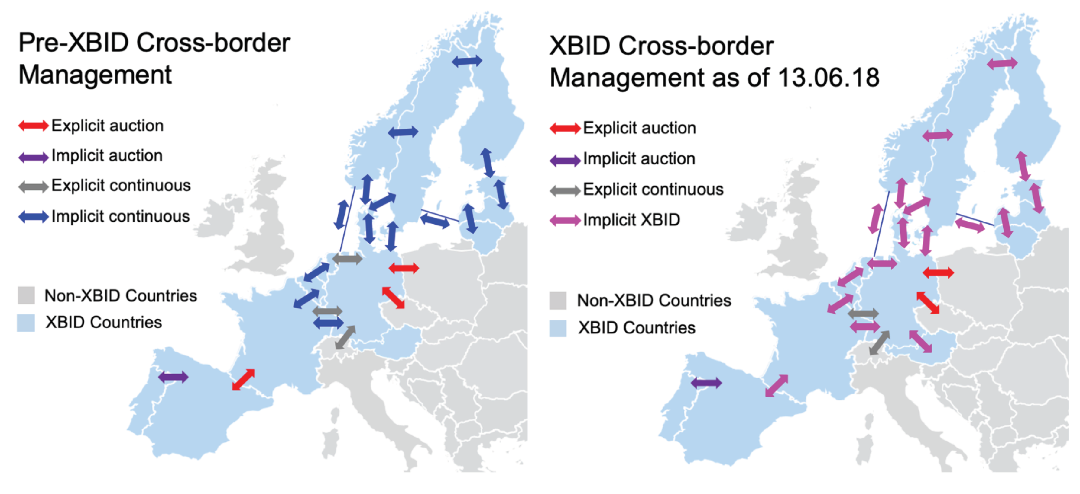
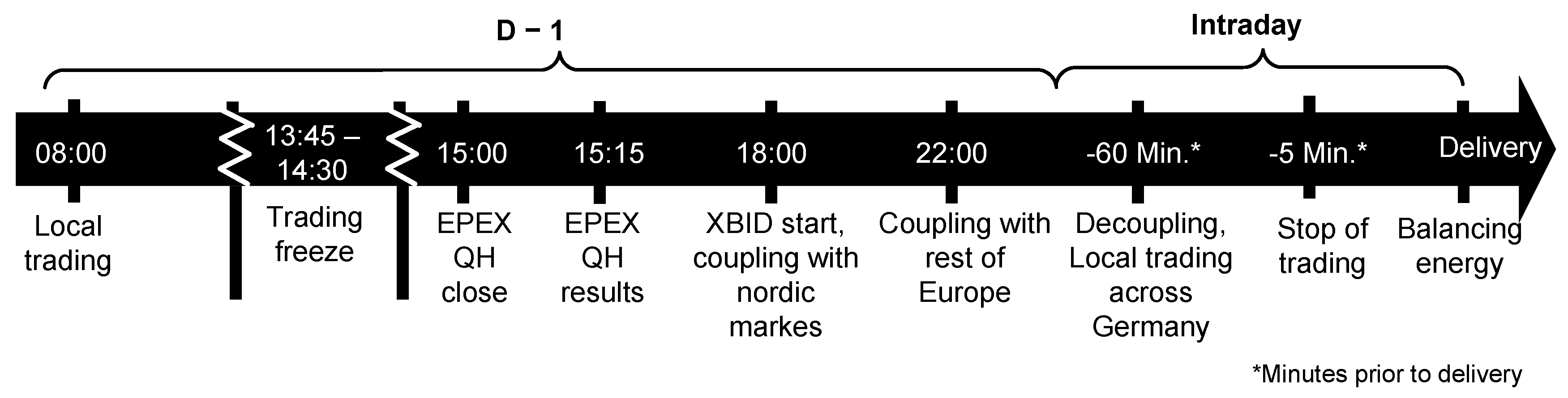
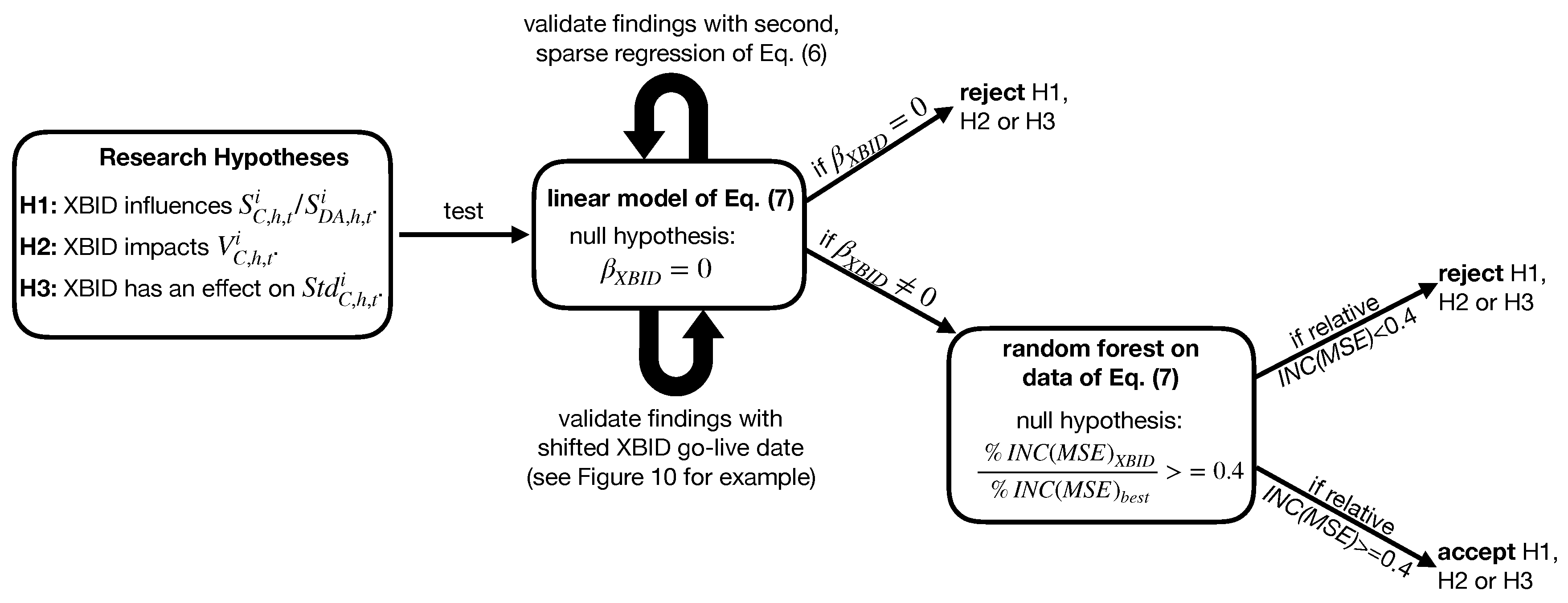
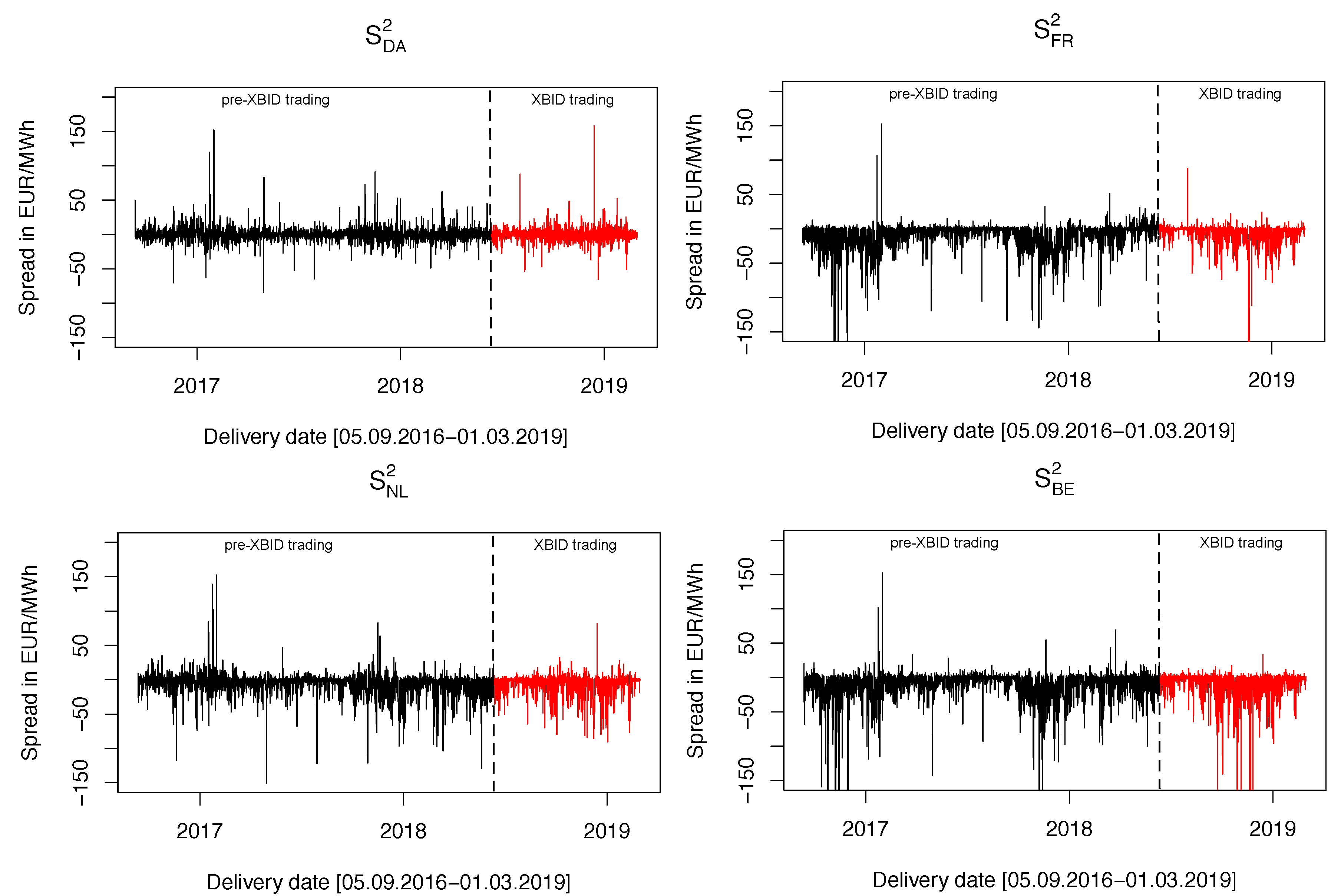
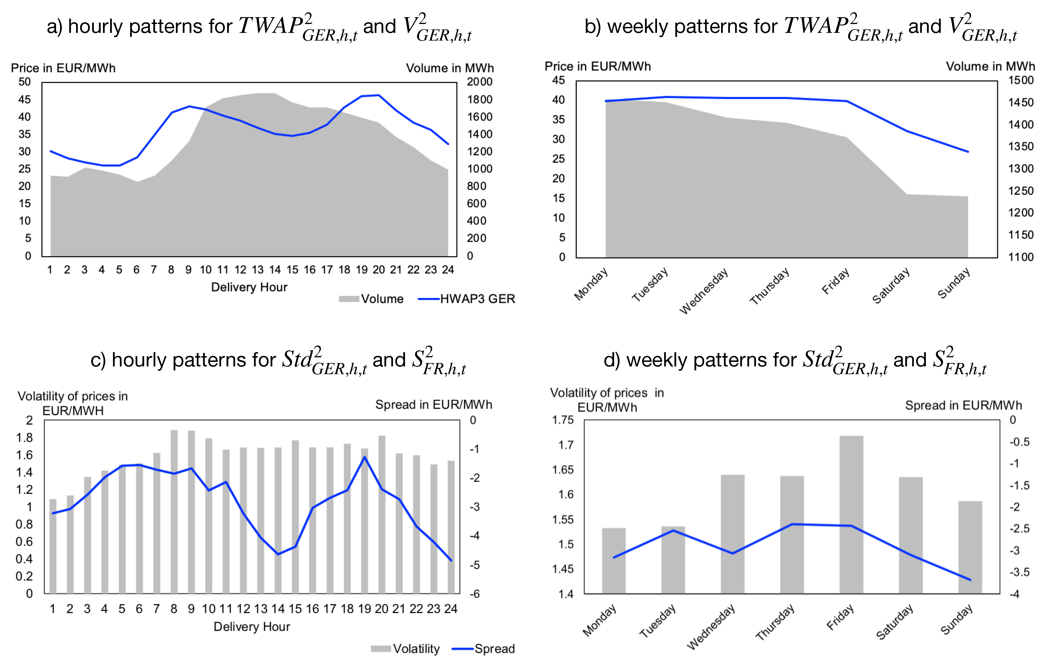
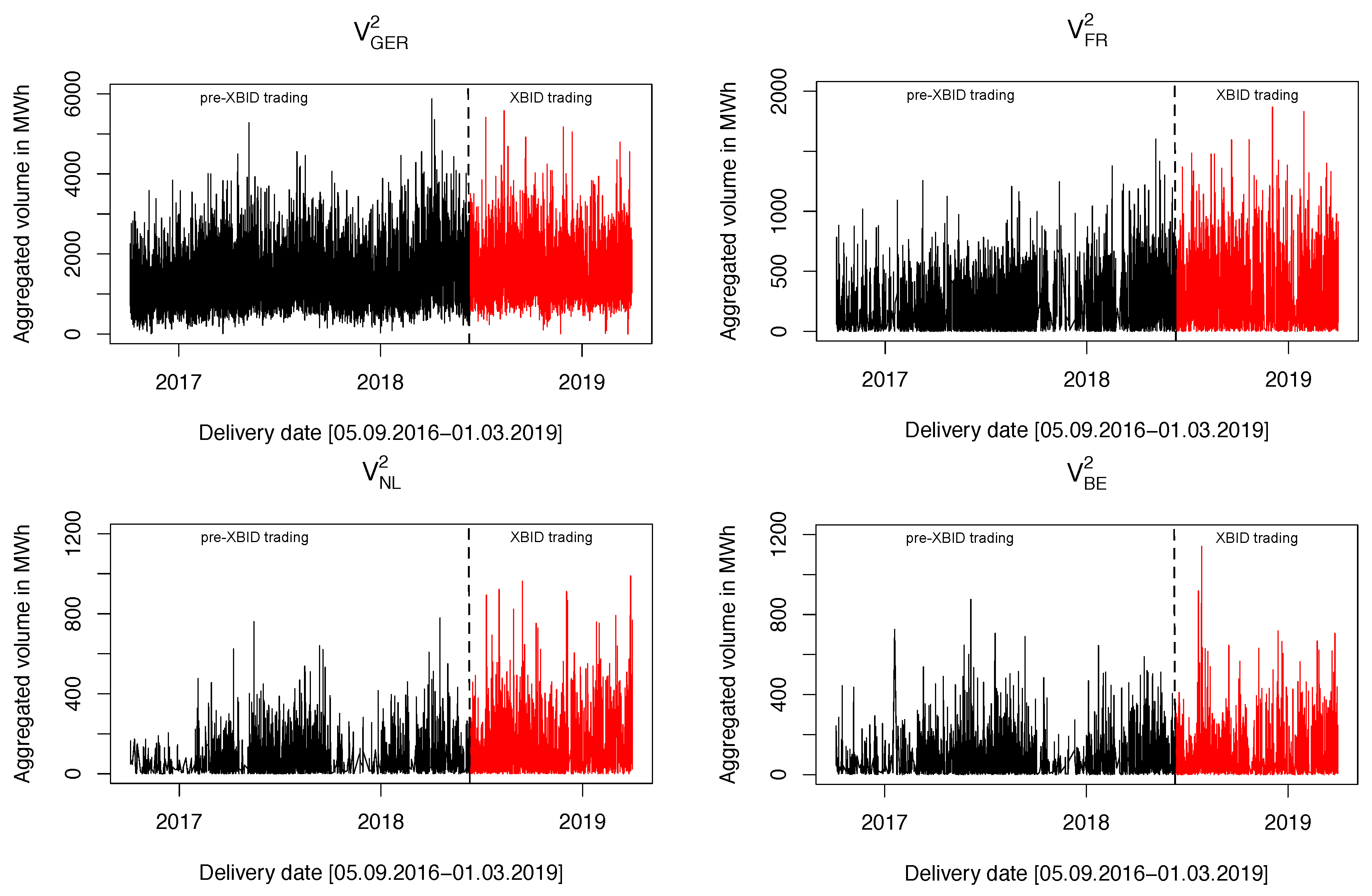
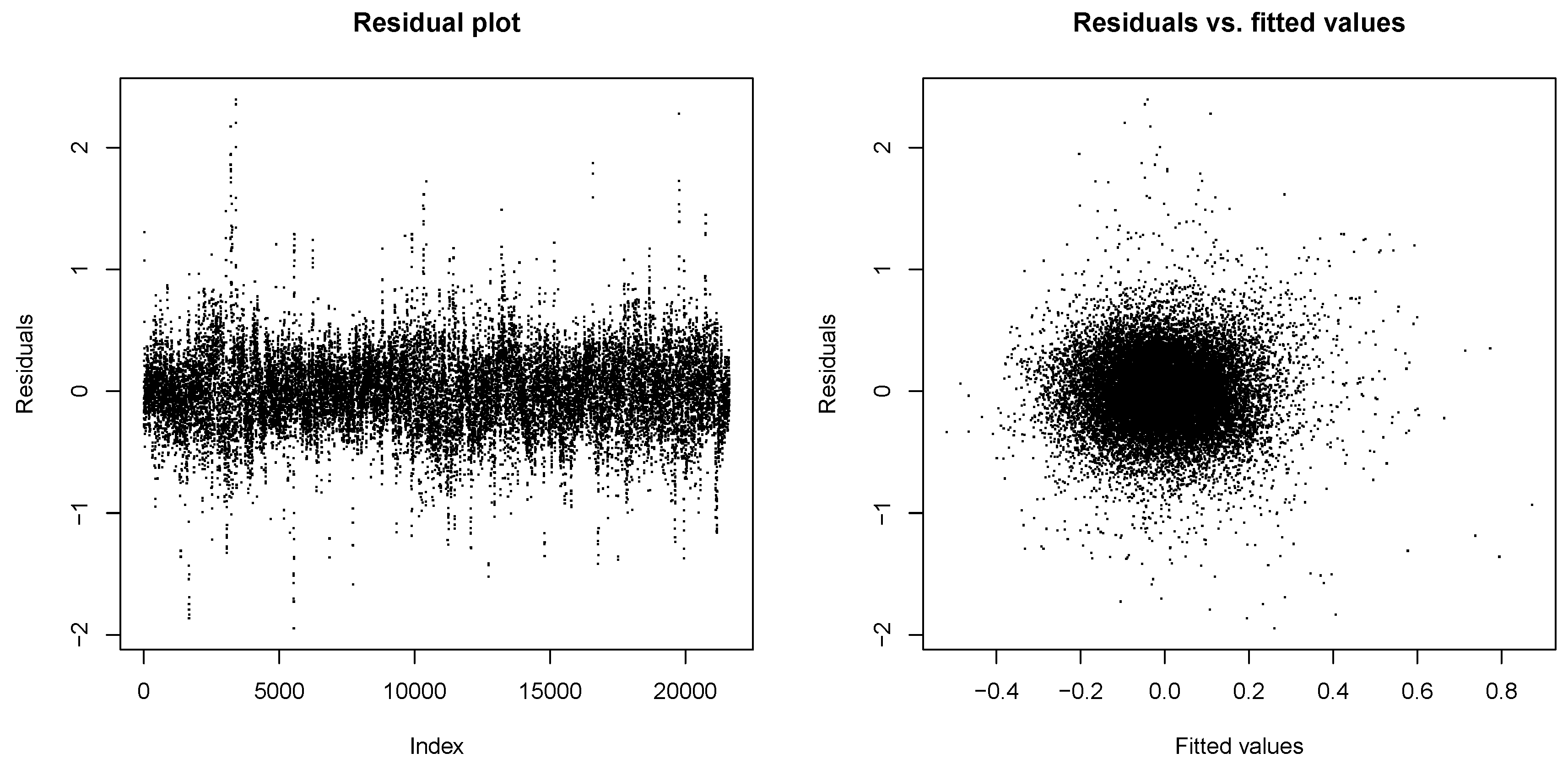
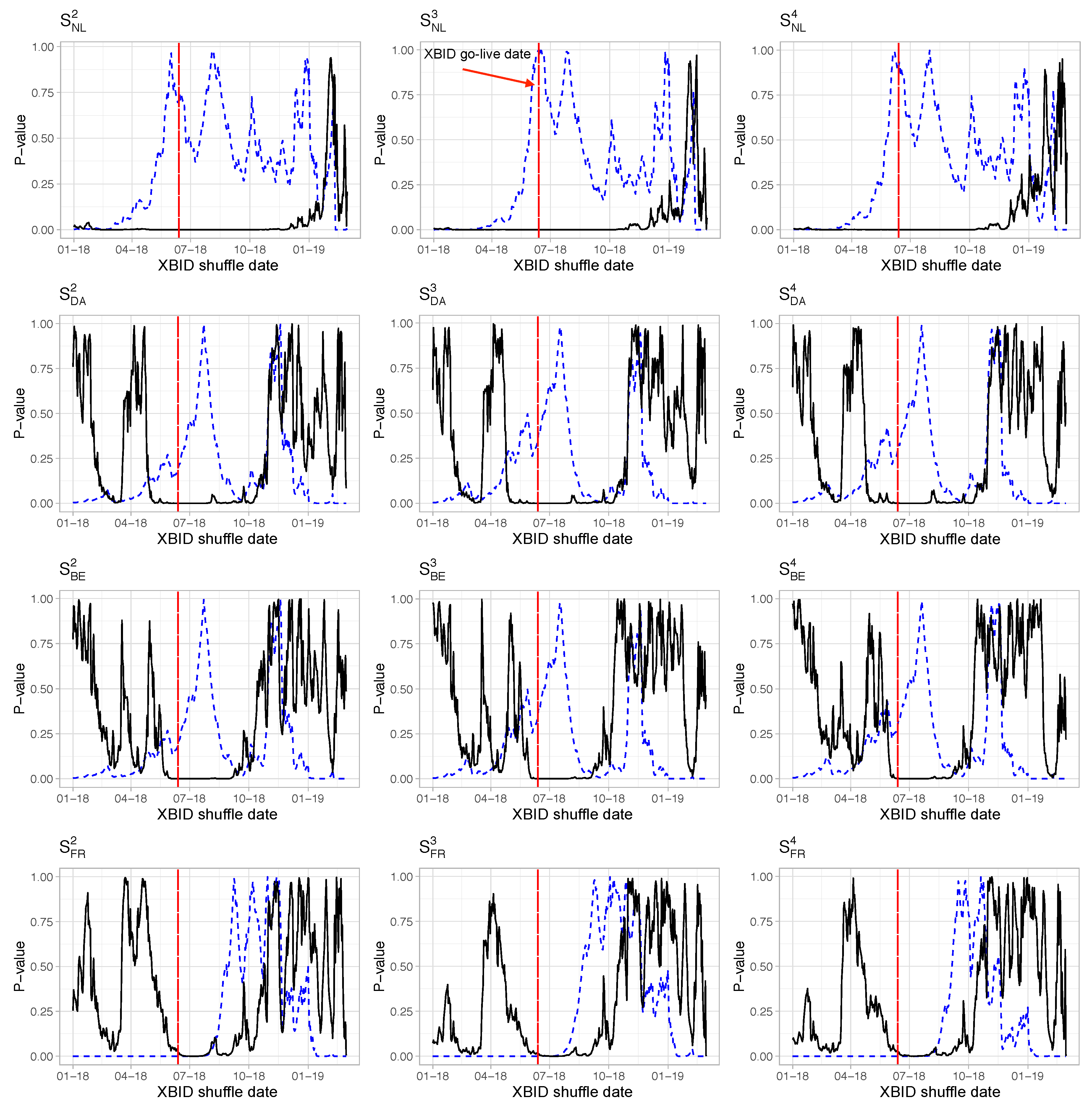
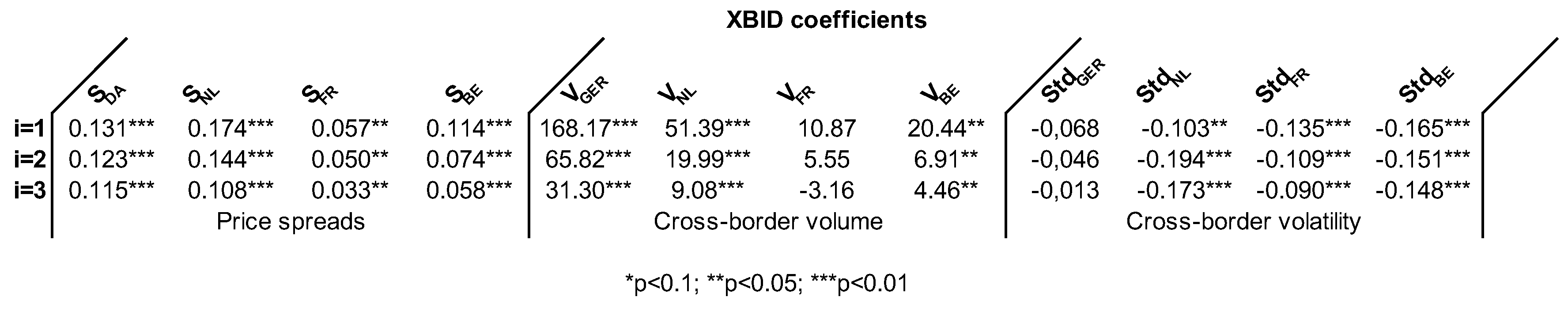
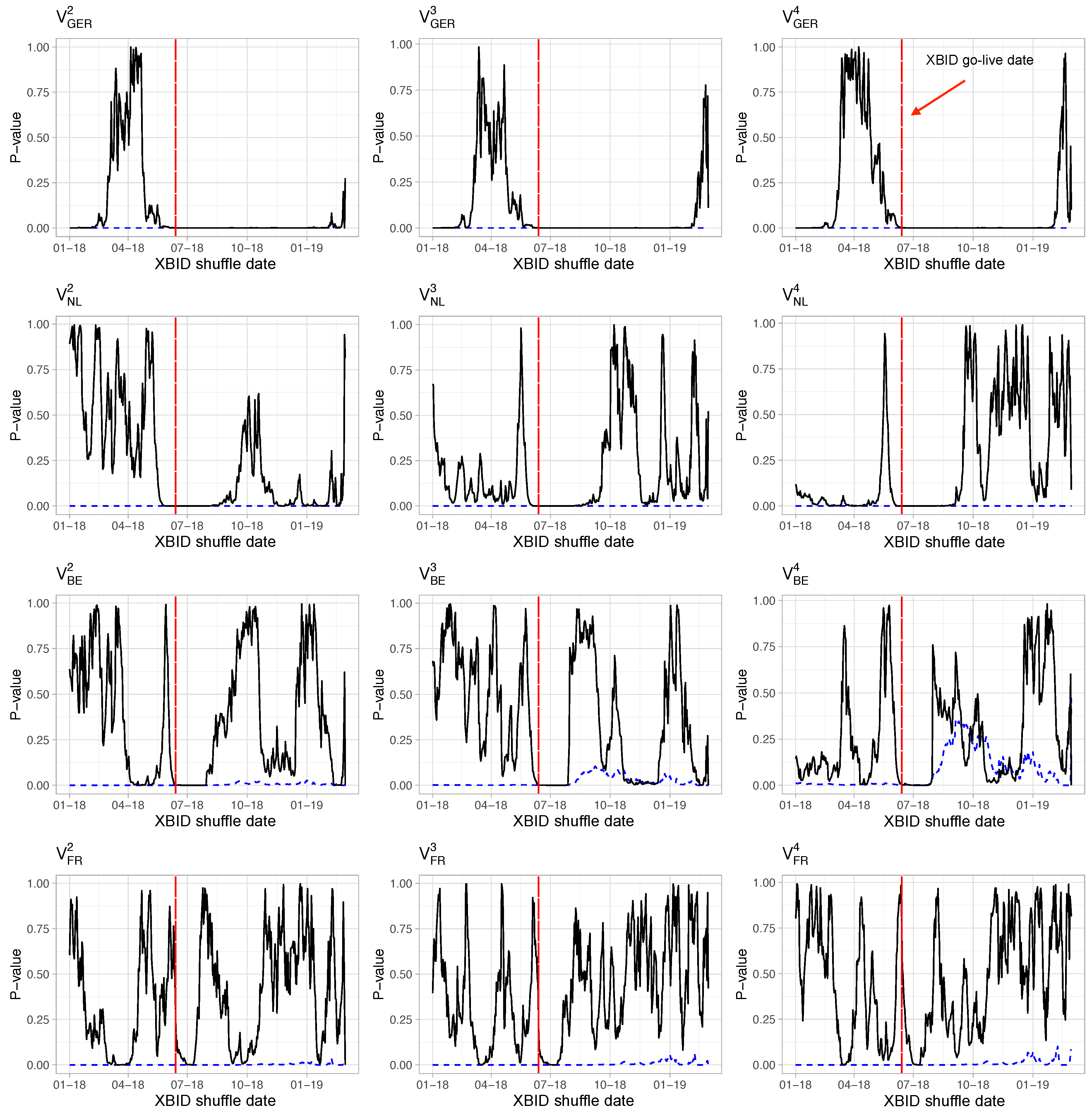
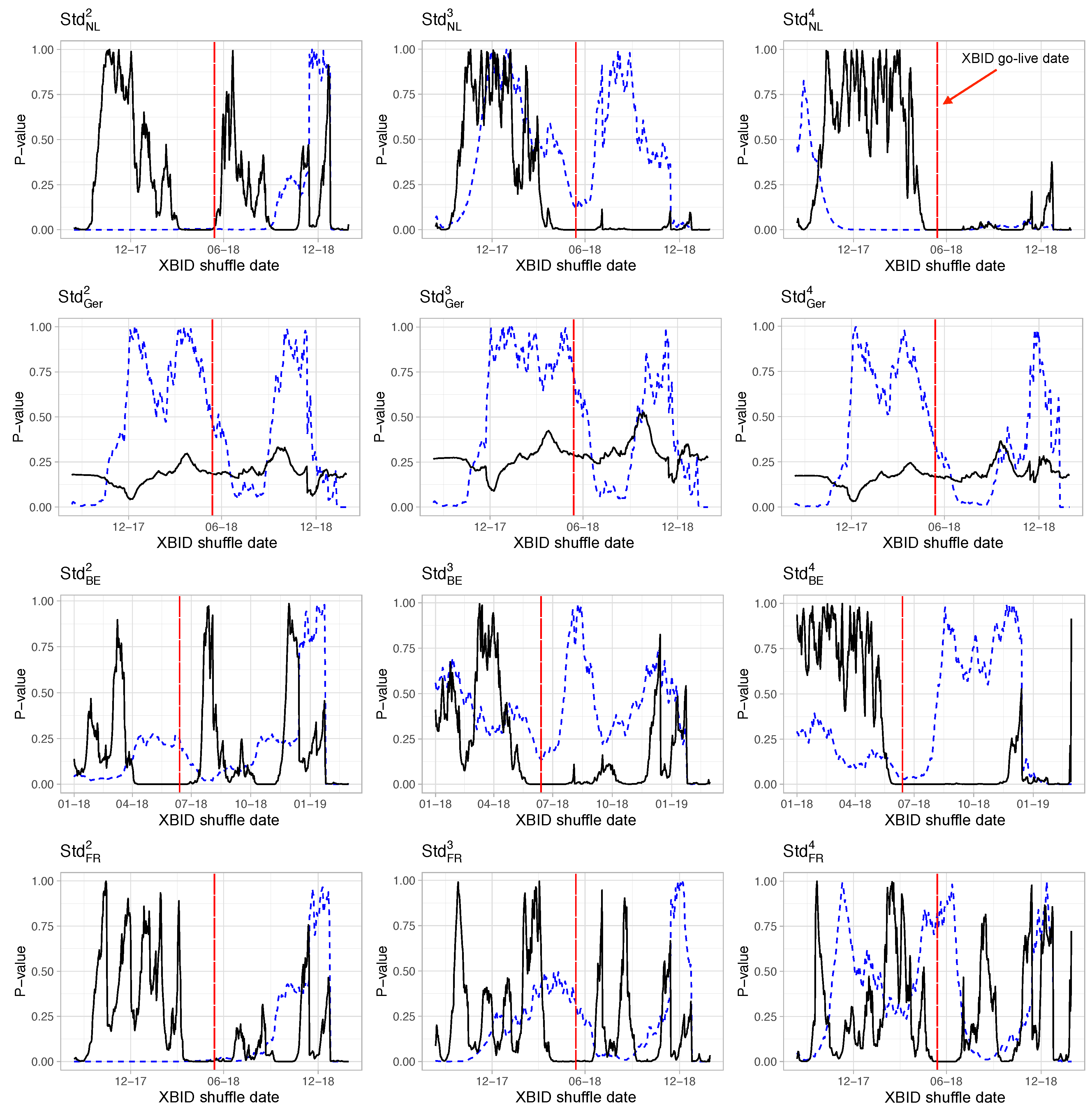
Table 1.
Total scheduled volume between Germany and its neighboring countries based on European Network of Transmission System Operators (ENTSO-E) data for the year 2018. Albeit Sweden and Germany share no border, they can be coupled via Denmark. Since the data source explicit reports such capacities, we will report them likewise.
| Country | AT | FR | NL | CZ | CH | DK | PL | SWE |
|---|---|---|---|---|---|---|---|---|
| Import from GER in GWh | 36.760 | 14.784 | 15.162 | 6.002 | 9.534 | 6.289 | 1.885 | 0.468 |
| Import to GER in GWh | 11.583 | 6.445 | 0.628 | 8.181 | 5.255 | 6.413 | 1.003 | 1.308 |
Table 2.
Country data filtering criteria for intraday price spreads mentioned in Section 3.2, cross-border volumes of Section 3.3 and volatility of Section 3.4. The variable C describes the country of choice, i.e., Germany, the Netherlands, Belgium, and France.
Table 2.
Country data filtering criteria for intraday price spreads mentioned in Section 3.2, cross-border volumes of Section 3.3 and volatility of Section 3.4. The variable C describes the country of choice, i.e., Germany, the Netherlands, Belgium, and France.
| Dimension | Data Selection | Condition |
|---|---|---|
| Intraday spreads | price, volume | |
| Cross-border volumes | volume | |
| Cross-border volatility | price, volume |
Table 3.
Descriptive statistics for day-ahead/intraday spreads with C being France, Belgium, and the Netherlands before mlog transformation.
Table 3.
Descriptive statistics for day-ahead/intraday spreads with C being France, Belgium, and the Netherlands before mlog transformation.
| Min | 1st Quantile | Mean | 3rd Quantile | Max | Std.Dev. | |
|---|---|---|---|---|---|---|
| −83.99 | 0 | 0.09 | 3.58 | 158.21 | 8.54 | |
| −650.02 | −15.97 | −10.82 | 0.03 | 158.46 | 20.4 | |
| −150.51 | −9.16 | −5.71 | 0.43 | 152.46 | 13.6 | |
| −820.18 | −14.42 | −9.11 | 0.06 | 152.46 | 18.3 |
Table 4.
Overview of applied explanatory variables, their characteristics and how to obtain them for the sake of reproducibility.
Table 4.
Overview of applied explanatory variables, their characteristics and how to obtain them for the sake of reproducibility.
| Determinant | Unit/granularity | Description | Data Source | Transformation |
|---|---|---|---|---|
| EPEX day-ahead auction price | EUR/MWh, hourly | Market clearing price of the EPEX day-ahead auction | European Power Exchange (EPEX), https://www.epexspot.com/en/ | mlog |
| foreign day-ahead price | EUR/MWh, hourly | Market clearing price for Denmark, Poland, France, Belgium, Switzerland, Czech Republic and Sweden. All prices obtained in a day-ahead auction | European Network of Transmission System Operators (ENTSO-E), https://transparency.entsoe.eu/ | mlog |
| EPEX intraday transactions | EUR/MWh, hourly | EPEX public trades to derive TWAPs, volume or volatility from | European Power Exchange (EPEX), https://www.epexspot.com/en/ | mlog |
| ENTSO-E flow | EUR/MWh, hourly | Scheduled commercial exchanges per country, published ex-post | European Network of Transmission System Operators (ENTSO-E), https://transparency.entsoe.eu/ | - |
| ENTSO-E load | MW, quarter-hourly | Vertical system load for bidding zone Germany/Austria, published around 10:00 d-1 | European Network of Transmission System Operators (ENTSO-E), https://transparency.entsoe.eu/ | mlog, sum of QH for one hour |
| TSO PV and wind forecast | MW, hourly | Photovoltaics (PV) and wind production forecast for Germany published by transmission system operators (TSO) at 8:00 d-1 | European Energy Exchange (EEX), https://www.eex-transparency.com/ | mlog |
| EUA future price | EUR/ton, daily | EEX EUA front-year future, closing price of each day | European Energy Exchange (EEX), https://www.eex.com/de/ | mlog |
| Coal future price | USD/ton, daily | ICE API2 Rotterdam front-month coal future, settlement price | Intercontinental Exchange (ICE), https://www.theice.com/index | mlog |
| Gas future price | EUR/MWh, daily | EEX Gaspool front-month gas future, settlement price | PEGAS https://www.powernext.com/ | mlog |
Table 5.
Regression quality test results for price spreads, volume and volatility. Please note that the countries Belgium, France and the Netherlands were not depicted in case of volume and volatility since their results do not differ from the ones shown. The same holds for time-stamp ranges .
Table 5.
Regression quality test results for price spreads, volume and volatility. Please note that the countries Belgium, France and the Netherlands were not depicted in case of volume and volatility since their results do not differ from the ones shown. The same holds for time-stamp ranges .
| ADF test | 0.01 | <0.01 | <0.01 | <0.001 | 0.01 | 0.01 |
| KPSS test | 0.1 | 0.01 | <0.01 | 0.01 | <0.001 | <0.001 |
| Durbin-Watson test | <0.001 | <0.001 | <0.001 | <0.001 | <0.001 | <0.001 |
| Breusch-Pagan test | <0.001 | <0.001 | 0.005 | 0.008 | <0.001 | <0.001 |
| F-Statistics | <0.001 | <0.001 | <0.001 | <0.001 | <0.001 | <0.001 |
Table 6.
Non-linear importance ranking based on random forest’s increase in mean-squared-error (MSE). The values in brackets report the increase in MSE (also denoted as %INC(MSE)) if the values of the respective regressor are permuted. In order to accept research hypothesis H1, the relation of the XBID dummy variable in comparison to the most informative variable must at least be . Please note that X->Y describes the ENTSO-E flow from country X to country Y.
| Rank (x of 46) | ||||
|---|---|---|---|---|
| 1 | GER DA PRC (26%) | NL DA PRC (117%) | FR DA PRC (154%) | BE DA PRC (427%) |
| 2 | DK–>GER (22%) | GER DA PRC (108%) | FR–>GER (102%) | FR–>GER (79%) |
| 3 | CH DA PRC (20%) | CZ DA PRC (30%) | CH DA PRC (55%) | GER DA PRC (74%) |
| 4 | GER–>DK (20%) | Wind FC (29%) | BE DA PRC (53%) | FR DA PRC (66%) |
| 5 | BE DA PRC (13%) | lagged PV FC (27%) | GER DA PRC (41%) | CH DA PRC (60%) |
| rank XBID | 46/(0.3%) | 45/(1.3%) | 39/(2.1%) | 45/(0.8%) |
Table 7.
Non-linear importance based on random forest’s percentage increase in MSE. The values in brackets report the increase in MSE (also denoted as %INC(MSE)) if the values of the respective regressor are permuted. In order to accept research hypothesis H2, the relation of the XBID dummy variable in comparison to the most informative variable must at least be . Please note that X->Y describes the ENTSO-E flow from country X to country Y.
| Rank (x of 46) | ||||
|---|---|---|---|---|
| 1 | FR–>GER (66 512%) | XBID (1 841%) | NL–>GER 1 759%) | FR–>GER (26 997%) |
| 2 | CH–>GER (31 341%) | EUA PRC (1 779%) | Load BE (1 010%) | CH–>GER (6 114%) |
| 3 | EUA PRC (21 4229%) | NL–>GER 1 750%) | DK DA PRC (851%) | GER DA PRC (75 244%) |
| 4 | AT–>GER (19 537%) | FR–>GER (19 537%) | BE DA PRC (762%) | FR DA PRC (4 556%) |
| 5 | DK DA PRC (15 921%) | GER DA PRC (1 218%) | GER DA PRC (729%) | DK DA PRC (4 190%) |
| rank XBID | 7/(14 447%) | 1/(1 841%) | 39/(653%) | 37/(132%) |
Table 8.
Non-linear importance ranking based on random forest’s increase in MSE for intraday price standard deviation. The values in brackets report the increase in MSE (also denoted as %INC(MSE)) if the values of the respective regressor are permuted. In order to accept research hypothesis H3, the relation of the XBID dummy variable in comparison to the most informative variable must at least be . Please note that X->Y describes the ENTSO-E flow from country X to country Y.
| Rank (x of 46) | ||||
|---|---|---|---|---|
| 1 | FR–>GER (3.3%) | GER DA PRC (0.9%) | GER DA PRC (1.2%) | GER DA PRC (0.6%) |
| 2 | CH–>GER (2.1%) | CZ DA PRC (0.8%) | BE DA PRC (0.7%) | Load DK (0.4%) |
| 3 | EUA PRC (1.6%) | Load CZ (0.7%) | FR DA PRC (0.6%) | BE DA PRC (0.4%) |
| 4 | Wind FC(1.1%) | Load DK (0.6%) | CH DA PRC (0.4%) | FR DA PRC (0.3%) |
| 5 | lagged PV Forecast FC (1%) | DK DA PRC (0.4%) | FR–>GER (0.3%) | CH DA PRC (0.2%) |
| rank XBID | 44/(0.3%) | 41/(0.01%) | 29/(0.03%) | 35/(0.02%) |
© 2019 by the author. Licensee MDPI, Basel, Switzerland. This article is an open access article distributed under the terms and conditions of the Creative Commons Attribution (CC BY) license (http://creativecommons.org/licenses/by/4.0/).
Share and Cite
MDPI and ACS Style
Kath, C. Modeling Intraday Markets under the New Advances of the Cross-Border Intraday Project (XBID): Evidence from the German Intraday Market. Energies 2019, 12, 4339. https://0-doi-org.brum.beds.ac.uk/10.3390/en12224339
AMA Style
Kath C. Modeling Intraday Markets under the New Advances of the Cross-Border Intraday Project (XBID): Evidence from the German Intraday Market. Energies. 2019; 12(22):4339. https://0-doi-org.brum.beds.ac.uk/10.3390/en12224339
Chicago/Turabian StyleKath, Christopher. 2019. "Modeling Intraday Markets under the New Advances of the Cross-Border Intraday Project (XBID): Evidence from the German Intraday Market" Energies 12, no. 22: 4339. https://0-doi-org.brum.beds.ac.uk/10.3390/en12224339
Note that from the first issue of 2016, this journal uses article numbers instead of page numbers. See further details here.