Day-Ahead vs. Intraday—Forecasting the Price Spread to Maximize Economic Benefits

Abstract

Recently, a dynamic development of intermittent renewable energy sources (RES) has been observed. In order to allow for the adoption of trading contracts for unplanned events and changing weather conditions, the day-ahead markets have been complemented by intraday markets; in some countries, such as Poland, balancing markets are used for this purpose. This research focuses on a small RES generator, which has no market power and sells electricity through a larger trading company. The generator needs to decide, in advance, how much electricity is sold in the day-ahead market. The optimal decision of the generator on where to sell the production depends on the relation between prices in different markets. Unfortunately, when making the decision, the generator is not sure which market will offer a higher price. This article investigates the possible gains from utilizing forecasts of the price spread between the intraday/balancing and day-ahead markets in the decision process. It shows that the sign of the price spread can be successfully predicted with econometric models, such as ARX and probit. Moreover, our research demonstrates that the statistical measures of forecast accuracy, such as the percentage of correct sign classifications, do not necessarily coincide with economic benefits.

1. Introduction

Over the last decade, many countries have experienced a dynamic development of intermittent renewable energy sources (RES), among which wind and solar play a central role. From 2005 to 2014, RES generation in the EU (28 countries) increased by 87.8%, from 495.7 GWh to 930.9 GWh. In 2016, it reached 29.6% of the total gross electricity generation. Increasing input of RES affects both the electricity market and the distribution system. On one hand, it results in the reduction of ${\mathrm{CO}}_2$ emissions and the decrease of wholesale electricity prices [1,2,3,4]. On the other hand, expanding RES creates new challenges for market participants. Electricity generated by wind or photovoltaic (PV) depends strongly on weather conditions and, hence, is volatile and difficult to forecast; see [5] for a comprehensive discussion. In some countries, such as Germany, RES generation is granted priority during the dispatch and receives a fixed feed-in tariff. As a result, the day-ahead prices are more prone to extreme behavior, such as spikes or negative values [6]. Finally, RES generation increases the risk of system imbalance, because an inelastic demand needs to be covered by a stochastic supply.

Nowadays, a major share of electricity is sold on power exchanges, such as Nord Pool or European Energy Exchange (EEX) in Europe, India Energy Exchanges (IEX) in Asia, and Pennsylvania New Jersey Maryland Interconnection LLC (PJM) or New York Independent System Operator (NYISO) in the US, where day-ahead contracts dominate. The day-ahead prices, which in Europe are also called ’spot prices’, are set around noon on the day preceding the delivery. In order to allow for adoption of trading contracts in the case of unplanned events and changing weather conditions, the day-ahead markets are complemented by intraday and balancing markets. The intraday markets, typically organized by power exchanges, take the form of auctions (e.g., in Spain) or continuous trading (e.g., in Germany). They allow purchasing and selling of electricity throughout the whole day, up to a few minutes before the physical delivery. The final balancing of the demand and supply is achieved through the balancing markets, which are controlled by system operators and aim at securing the system stability. However, in some countries, such as Poland, they are used for short term transactions, instead of the intraday markets.

The structural changes in electricity markets influence the decision process of generation utilities. This research focuses on a small RES generator, which has no market power and, hence, is a price taker. This type of a utility typically sells electricity through a larger trading company. The generator needs to decide, in advance, how much electricity will be sold in the spot market. If it offers a quantity smaller than the actual production, then the excess generation is traded in the intraday or the balancing market. On the contrary, if the offered quantity is larger than the actual one, then the RES generator needs to purchase the electricity to meet the day-ahead contracts. The optimal decision of the generator on where to sell the production depends on the relation between prices in these markets [7,8]. Unfortunately, when making the decision, the generator faces the uncertainty about the production and the price levels. Hence, it is not sure if it is able to produce the proposed quantity and which market offers a higher price. This article addresses the second question and investigates the possible gains from utilizing forecasts of the price spread between the day-ahead and the intraday/balancing market in the decision process.

There is a rich literature on forecasting electricity prices; see [5] and [9,10] for comprehensive reviews of point and probabilistic forecasts, respectively. However, the majority of articles focus on day-ahead prices, since they have the longest history and are perceived as a benchmark for various financial instruments. A variety of prediction methods were proposed, ranging from linear, univariate time series models [11], neural networks [12], and Lasso regressions [13], to multivariate models [14,15] and forecast averaging [16,17]. The literature indicates that RES generation is one of the most important drivers of the spot price level [1,4,18] and distribution [19]. The intraday prices have not been studied as intensively as their day-ahead counterparts. There are a few articles which analyzed the intraday markets in Germany [13,20,21], Spain [12], and the US [4]. They linked the intraday prices with RES forecast errors [18,22,23]. Unfortunately, typically the research focuses only on short-term forecasts and, hence, assumes the knowledge of the day-ahead prices [4].

This article extends the literature in various directions. First, we consider the point of view of a small generator, which needs to choose an optimal trading strategy by comparing predicted prices in different markets. Hence, the day-ahead and the intraday/balancing prices have to be forecasted jointly. We show that the sign of the price spread, which is crucial for the decision process, can be successfully predicted with econometric models. Second, we examine different model specifications, which vary in terms of the aggregation level (hourly versus daily data), the choice of exogenous variables, the lag structure, and the length of the estimation window. We show that although the disaggregated, hourly data provides more information, it does not lead to more efficient forecasts than the aggregated, daily approach. Moreover, the results indicate that the fundamentals—in particular, RES generation—impact not only the level of prices but also the price spread, and that they are useful in formulating an optimal trading strategy. Finally, we demonstrate that the statistical measures of forecast accuracy, such as the classification power, do not necessarily coincide with economic gains. Similar to [13,24], we encourage a deeper look at the financial benefits of prediction methods.

The rest of the paper is structured as follows. In Section 2, we describe the data used for modeling the Polish and the German electricity markets. In Section 3, we introduce the econometric methods employed in the analysis and discuss forecast evaluation. We present the results in Section 4. Finally, in Section 5, we conclude the study.

2. Data

This article analyzes two distinct electricity markets: Germany and Poland. Although they are both located in Europe and are neighbors, they differ in terms of the generation structure and the market organization. Germany is well known for its success in RES penetration, which—at the time of this article—accounts for 40.2% of total electricity production (see https://www.energy-charts.de). At the same time, Polish electricity generation is based on coal, with RES reaching only 8.4% (see https://www.pse.pl/dane-systemowe/funkcjonowanie-kse/raporty-miesieczne-z-funkcjonowania-rb/raporty-miesieczne). In both countries, RES has priority during the dispatch. Second, the German and Polish markets are designed differently, which could affect the decision process of market participants [8]. The intraday market in Germany is based on the pay-as-bid principle, which has been complemented by intraday auctions. In Poland, the balancing market, which is considered as the main market for contract adjustments, uses a double price approach. The practice shows, however, that a single market-clearing price is preferred by the market operator and, hence, the double prices have never been applied. Finally, in Germany, negative prices are allowed in both day-ahead and intraday markets, whereas, in Poland, until 2019 the balancing prices were restricted to be positive and to stay within an interval of 70–500 PLN/MWh (which is equivalent to 17.5–125 EUR/MWh). A recent regulation, which came into power on 1 January 2019, changed the lower and the upper bounds to −50,000 PLN/MWh and 50,000 PLN/MWh, respectively.

The data used in this research is hourly and spans the period from 1 January 2016 to 31 December 2017. The data for Poland consists of day-ahead and balancing market prices (both in Polish zloty, PLN). The prices are complemented by exogenous variables: The forecasted energy demand, the forecasted wind generation, and the forecasted available energy reserves. The intraday prices are not included in the analysis, as the market is not liquid. The German data is comprised of energy prices (in Euros) in the day-ahead and intraday markets. The intraday prices are calculated as the weighted average of all intraday contracts for the given hour. The exogenous variables are: The forecasted total load, which can be treated as a proxy for the forecasted demand, and the forecasted wind generation. Data sources and units are summarized in

Table 1. Data sources.

Data	Notation	Units	Source
Poland
Day-ahead prices	$P^0$	PLN/MWh	TGE S.A., https://www.tge.pl
Balancing prices	$P^1$	PLN/MWh	PSE S.A., http://www.pse.pl
Forecasted demand	$X_1$	MWh	PSE S.A., http://www.pse.pl
Forecasted wind generation	$X_2$	MWh	PSE S.A., http://www.pse.pl
Forecasted reserves	$X_3$	MWh	PSE S.A., http://www.pse.pl
Germany
Day-ahead prices	$P^0$	EUR/MWh	EPEX SPOT, http://www.epexspot.com
Intraday prices	$P^1$	EUR/MWh	EPEX SPOT, http://www.epexspot.com
Forecasted load	$X_1$	MWh	https://transparency.entsoe.eu
Forecasted wind generation	$X_2$	MWh	https://transparency.entsoe.eu

.

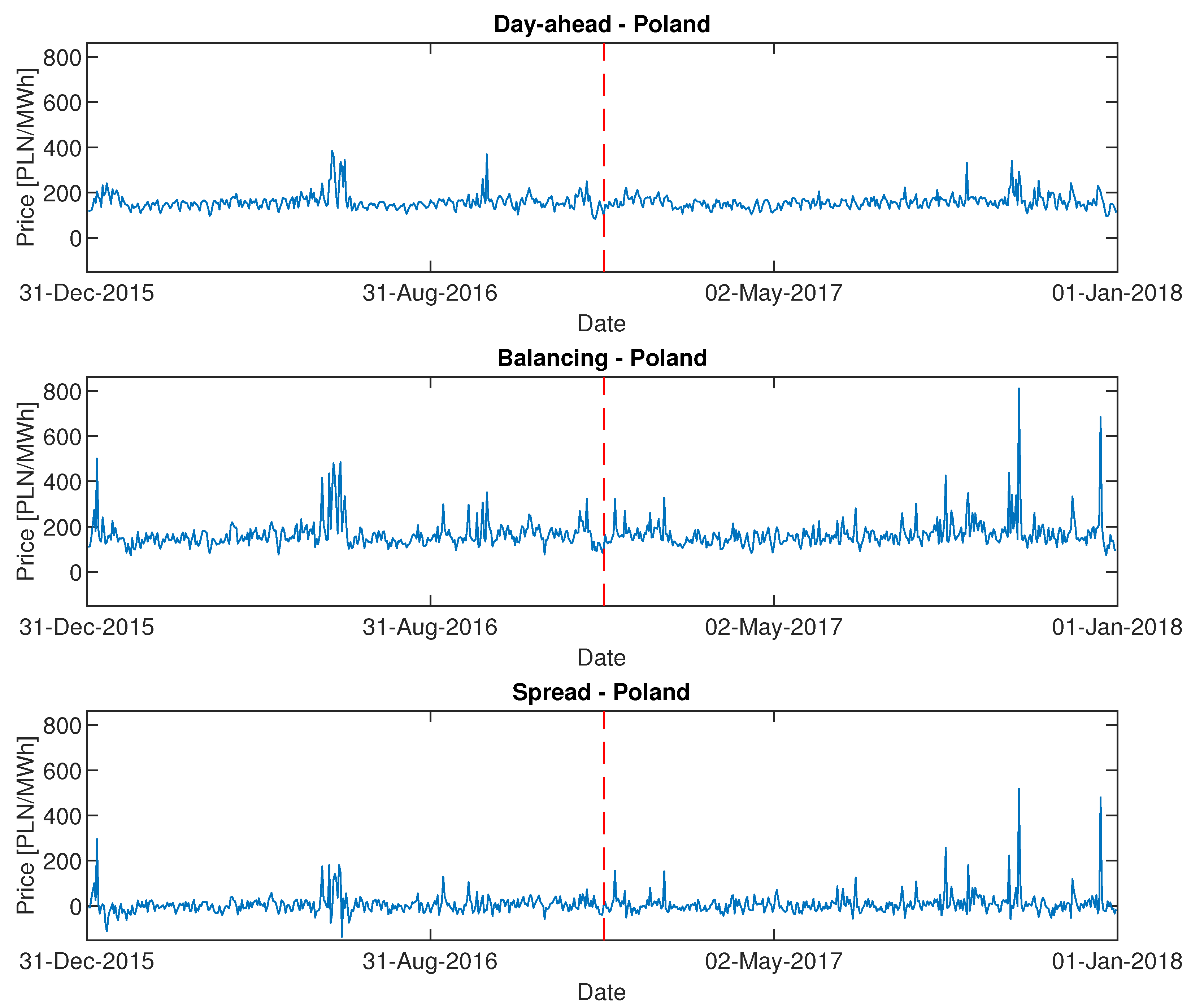
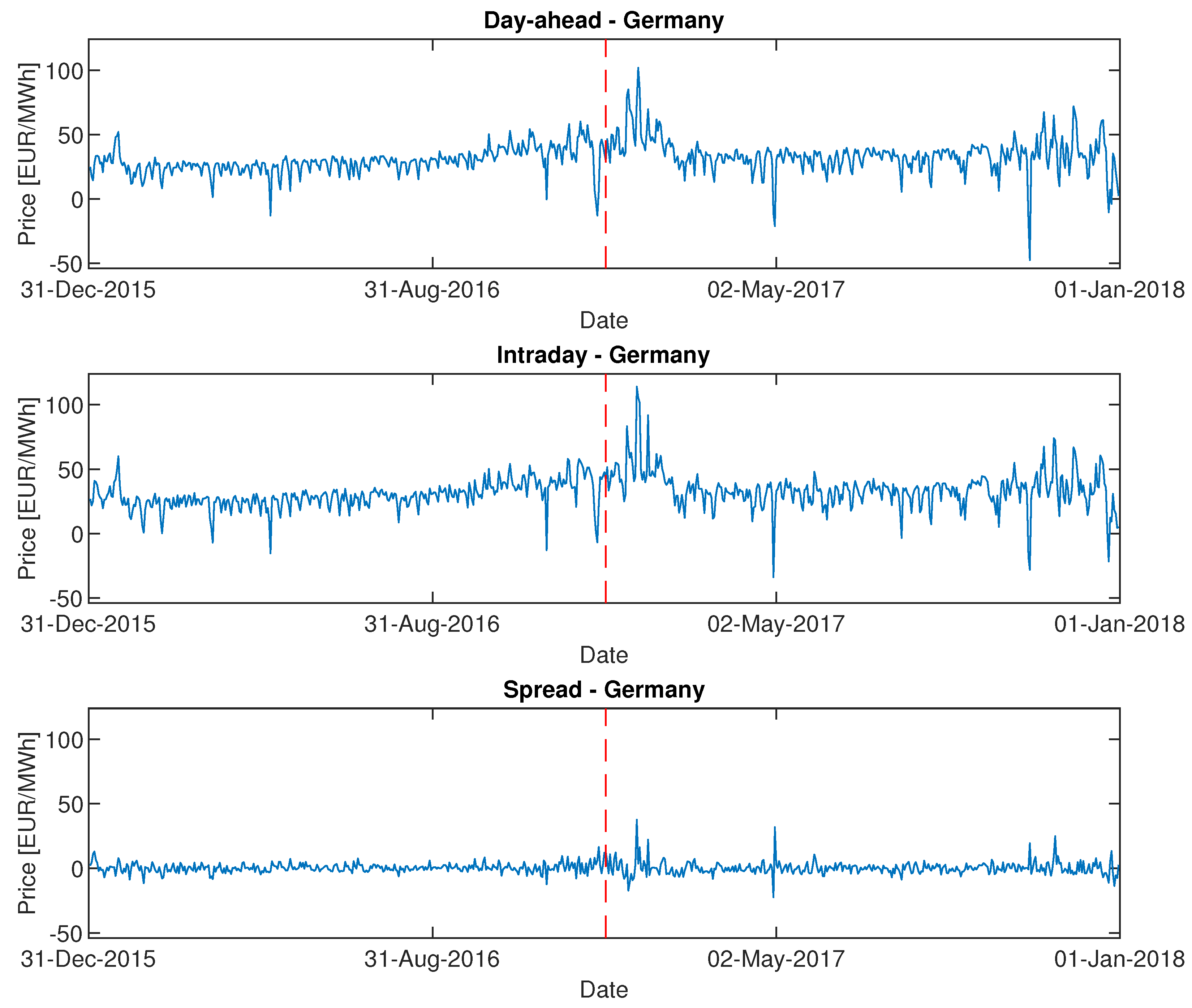
Time paths of electricity price, together with the price spread, computed as the excess of the intraday/balancing price over the spot price, are presented in Figure 1 and Figure 2. First, it can be observed that the day-ahead prices are less volatile than the intraday/balancing prices, especially for Poland. Moreover, both time series are characterized by positive spikes, with Germany exhibiting sudden drops with prices falling below zero. Spikes are also observed in the spread series, indicating that they are not perfectly synchronized between markets. The basic descriptive statistics of electricity prices are presented in

Table 2. Mean and standard deviation (Std. dev.) of the energy prices.

Country	Market	Mean	Std. dev.
	Day-ahead	158.51	33.424
Poland	Balancing	165.717	61.138
	Spread	7.198	45.009
	Day-ahead	31.580	12.293
Germany	Intraday	31.754	13.057
	Spread	0.174	4.494

. They confirm that balancing and intraday prices are, on average, higher and more volatile than day-ahead prices, with the difference being more pronounced for Poland. Finally, it could be noticed that the spread in Germany has a much lower variance than any of the prices, whereas, in Poland, the spread is more volatile than spot prices.

In order to evaluate the forecasting possibilities of the price difference, the sample is divided into estimation and validation periods. The validation window contains the last 365 observations, from 1 January 2017 to 31 December 2017 (see Figure 1 and Figure 2). In this research, a rolling estimation window approach was adopted, with its length ranging from a month (30 days), a quarter (91 days), half a year (182 days), to a year (365 days).

3. Forecasting Methods and Forecast Evaluation

In order to model market preference, let us define a decision variable $Y_{ht}$, which equals one when the generator decides to sell the electricity for hour h and day t in the intraday market, and zero otherwise. Let us consider two benchmark strategies: The first one assumes that the utility sells all generated electricity in the day-ahead market. In such a case, $Y_{ht}=0$ for all h and t. The second one assumes that the generator enters only the intraday/balancing market and, hence, it is always the case that $Y_{ht}=1$. We refer to them as naïve day-ahead and naïve intraday/balancing strategies, respectively. Here, we compare them with a data driven approach, which assumes that the decision depends on the relationship between the day-ahead ($P_{ht}^0$) and the intraday/balancing price ($P_{ht}^1$)

$$Y_{ht}=\left\{\begin{array}{c}1\mathrm{if}{P}_{ht}^1>P_{ht}^0,\hfill \\ 0\mathrm{if}{P}_{ht}^1\le P_{ht}^0.\hfill \end{array}\right.$$

(1)

As the price difference $\Delta P_{ht}=P_{ht}^1-P_{ht}^0$ is not known in advance, the generator needs to base its decision on the predicted spread

$${\widehat{Y}}_{ht}=\left\{\begin{array}{c}1\mathrm{if}\Delta {\widehat{P}}_{ht|t-1}>0,\hfill \\ 0\mathrm{if}\Delta {\widehat{P}}_{ht|t-1}\le 0\hfill \end{array}\right.,$$

(2)

where $\Delta {\widehat{P}}_{ht|t-1}$ is a forecast of $\Delta P_{ht}$, computed using the information available on day $t-1$. In this research, two alternative ways of forecasting $Y_{ht}$ are considered. First, autoregressive models with exogenous variables (ARX) are examined, which either (1) separately model the level of prices $P_{ht}^0$ and $P_{ht}^1$ and then compute $\Delta P_{ht}$, or (2) describe directly the price spread, $\Delta P_{ht}$. In the regression, information on predicted market fundamentals and past levels of prices is used. The forecast, ${\widehat{Y}}_{ht}$, is based on the sign of the predicted spread $\Delta {\widehat{P}}_{ht}$. Second, probit models are used, which describe directly the distribution of the binomial variable $Y_{ht}$ defined by (1). Similar to ARX models, the probability $\mathrm{Prob}(Y_{ht}=1)$ is conditioned on exogenous variables and lagged prices. A more detailed description of the models is presented in Section 3.1 and Section 3.2.

When the aggregated, daily models are considered, then the endogenous and exogenous variables are constructed as the daily averages of the corresponding hourly variables. The decision variable $Y_t$ becomes

$$Y_t=\left\{\begin{array}{c}1\mathrm{if}{P}_t^1>P_t^0\hfill \\ 0\mathrm{if}{P}_t^1\le P_t^0\hfill \end{array}\right.,$$

(3)

which implies that the generator adopts the same strategy throughout the day, and hence $Y_{1t}=\dots =Y_{24t}=Y_t$.

In the remaining part of the article, the following notation is used:

• $D_t$ denotes a $(4\times 1)$ vector of deterministic variables: A constant and dummy variables for Mondays, Saturdays, and Sundays/Holidays,
• $X_{ht}$ represents a vector of exogenous variables, which is a subset of $\{X_{1,ht}.X_{2,ht},X_{3,ht}\}$ for Poland and $\{X_{1,ht},X_{2,ht}\}$ for Germany. Variables $X_i$ are defined in Table 1.
• $X_t$, $P_t^0$, and $P_t^1$ are daily averages of the corresponding hourly variables: $X_{ht}$, $P_{ht}^0$, and $P_{ht}^1$, respectively.

3.1. Autoregressive Models

ARX is a linear model, which links the current level of an endogenous variable with its past values and a vector of exogenous variables. It has been widely applied in the literature and has proved useful in forecasting electricity prices; see [5] for a discussion. Here, two model specifications are considered. First, the prices $P_{ht}^0$ and $P_{ht}^1$ are modeled separately

$$P_{ht}^0=\alpha D_t+\beta X_{ht}+\sum _{i\in L\cup \left\{1\right\}}{\theta }_i{P}_{ht-i}^0+{ϵ}_{ht},$$

(4)

$$P_{ht}^1=\alpha D_t+\beta X_{ht}+\sum _{i\in L}{\theta }_i{P}_{ht-i}^1+\gamma P_{ht-1}^0+{ϵ}_{ht}.$$

(5)

Then, the spread $\Delta P_{ht}$ is computed as their difference: $\Delta P_{ht}=P_{ht}^1-P_{ht}^0$. Alternatively, the price spread is modeled directly, according to the following formula

$$\Delta P_{ht}=\alpha D_t+\beta X_{ht}+\sum _{i\in L}{\theta }_i\Delta P_{ht-i}+\gamma P_{ht-1}^0+{ϵ}_{ht}.$$

(6)

In both model specifications, $\alpha$ and $\beta$ are vectors of coefficients corresponding to the deterministic and exogenous variables, respectively, while ${\theta }_i$ are the autoregressive parameters and ${ϵ}_t$ are the residuals. Lags i belong to the pre-defined set L. Unfortunately, on day $t-1$, not all prices $P_{ht-1}^1$ are known yet, nor the spreads $\Delta P_{ht-1}$. For this reason the lag $i=1$ is excluded from set L, except when modeling $P_{ht}^0$. In order to compensate for this, the previous day’s price $P_{ht-1}^0$ is added to Equations (5) and (6).

Since the main interest of the generator is the optimal choice of the market, the results of regressions (4)–(6) are used to predict ${\widehat{Y}}_{ht}$. According to Equation (2), the utility sells in the intraday/balancing market, ${\widehat{Y}}_{ht}=1$, when the predicted spread $\Delta {\widehat{P}}_{ht}$ is positive. Otherwise, it chooses the day-ahead market, ${\widehat{Y}}_{ht}=0$.

For aggregated, daily models, the hourly observations in Equations (4)–(6) are replaced by their daily averages: $X_t$, $P_t^0$, $P_t^1$, and $\Delta P_t$. The structure of the models remains unchanged. As a result, the decision variable $Y_t$, defined by (3), is equal to one when $\Delta {\widehat{P}}_t>0$, and zero otherwise.

Parameters $\alpha$, $\beta$, ${\theta }_i$, and $\gamma$ are estimated with the least-squares (LS) method. For each hour, h, separately, the model is fitted such that the sum-of-squares of the differences between the observed and predicted values is minimized.

3.2. The Probit Model

The probit model is used to describe directly the probability distribution of the binary variable $Y_{ht}$. The model is formulated as follows:

$$\mathrm{Prob}(Y_{ht}=1|{\mathsf{\Omega }}_{t-1})=\mathsf{\Phi }\left(\alpha D_t+\beta X_{ht}+\sum _{i\in L}{\theta }_i\Delta P_{ht-i}+\gamma P_{ht-1}^0\right),$$

(7)

where $\mathsf{\Phi }\left(x\right)$ is the standard normal cumulative distribution function, $\alpha$ is a $(1\times 4)$ vector of parameters describing the impact of deterministic variables, and $\beta$ summarizes the effect of the exogenous variables. Finally, ${\theta }_i$ are the autoregressive parameters, with lags i belonging to the pre-defined set L, as in Equations (4)–(6). In order to utilize all the information available on day $t-1$, the effect of $P_{ht}^0$ on the probability is added by use of the parameter $\gamma$.

Parameters $\alpha$, $\beta$, ${\theta }_i$, and $\gamma$ are estimated separately for each hour, h, using the maximum likelihood method. Due to the lack of a closed-form solution for the maximization problem, the parameters are estimated numerically, using the Nelder-Mead algorithm [25]. Calculations are conducted in the R environment. The initial parameters for the procedure are estimated by a least-squares method and the number of iterations is limited to $\mathrm{10,000}$.

With parameter estimates $\widehat{\alpha }$, $\widehat{\beta }$, $\widehat{{\theta }_i}$, and $\widehat{\gamma }$ obtained within the rolling calibration window, the forecast of $Y_{ht}$ is defined as

$${\widehat{Y}}_{ht}=\left\{\begin{array}{c}1\mathrm{if}\mathsf{\Phi }\left(\widehat{\alpha }{D}_t+\widehat{\beta }{X}_{ht}+\sum _{i\in L}\widehat{{\theta }_i}\Delta P_{ht-i}+\widehat{\gamma }{P}_{ht-1}^0\right)>\mu ,\hfill \\ 0\mathrm{if}\mathsf{\Phi }\left(\widehat{\alpha }{D}_t+\widehat{\beta }{X}_{ht}+\sum _{i\in L}\widehat{{\theta }_i}\Delta P_{ht-i}+\widehat{\gamma }{P}_{ht-1}^0\right)\le \mu \hfill \end{array}\right.,$$

(8)

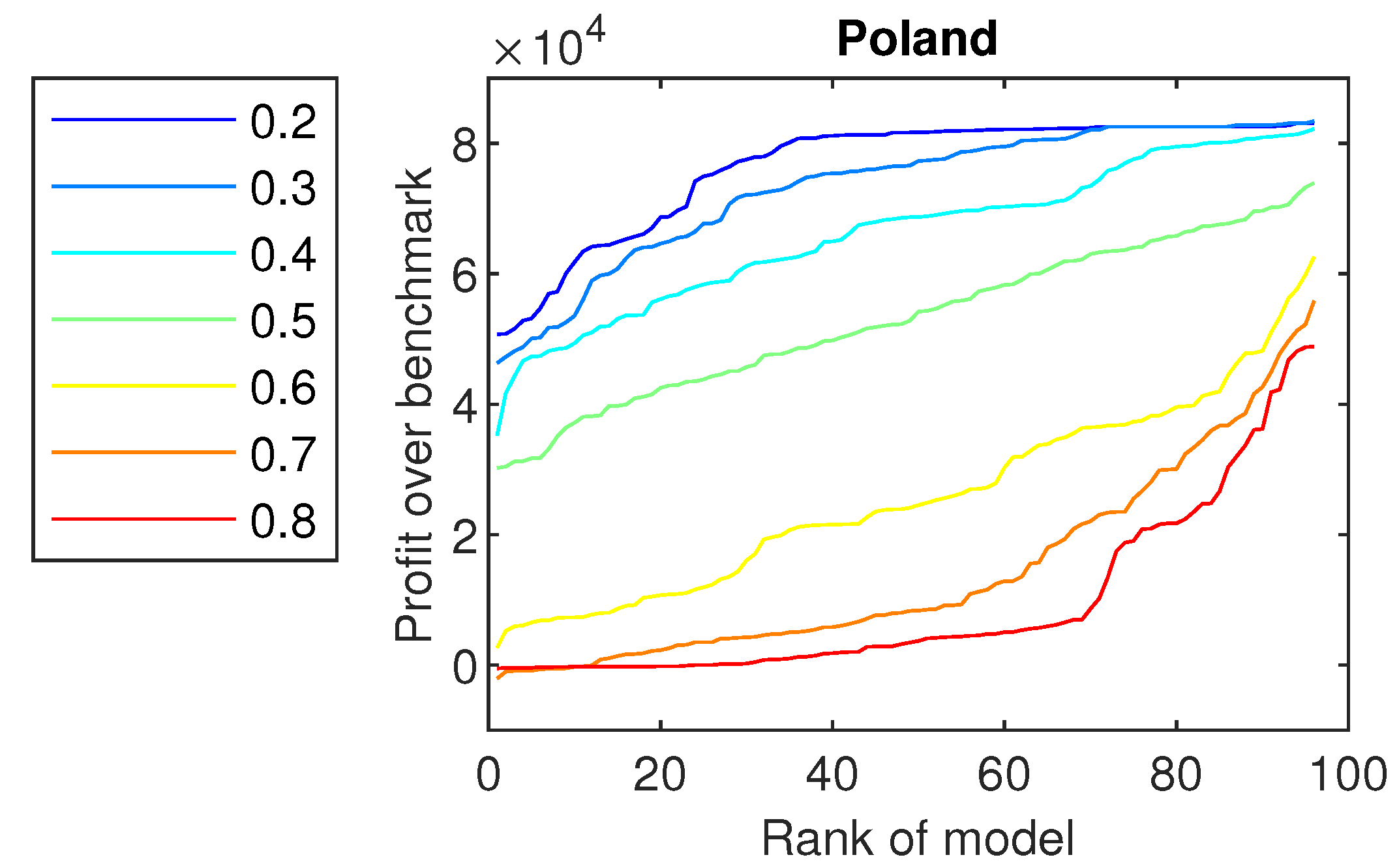
where $\mu \in \left(\mathrm{0,1}\right)$ is the threshold parameter. Typically, the threshold is chosen to equal $\mu =0.5$. However, the results indicated that $\mu =0.4$ or $\mu =0.3$ provide more accurate and profitable forecasts (see Section 4 for details).

For aggregated, daily models, Formula (7) becomes

$$\mathrm{Prob}(Y_t=1|{\mathsf{\Omega }}_{t-1})=\mathsf{\Phi }\left(\alpha D_t+\beta X_t+\sum _{i\in L}{\theta }_i\Delta P_{t-i}+\gamma P_{t-1}^0\right),$$

(9)

with the parameters defined as above. The forecasts ${\widehat{Y}}_t$ are obtained, as in (8), by comparing the forecasted probability with the threshold $\mu$.

3.3. Forecast Evaluation

The literature proposes various methods, which could be used to evaluate the accuracy of binomial variable forecasts. First, one could compute the classification power, denoted here by p:

$$p=\frac{1}{HT}\sum _{h=1}^H\sum _{t=1}^T{1}_{\{Y_{ht}={\widehat{Y}}_{ht}\}},$$

(10)

where $H=24$, $T=365$, and $1_{\left\{s\right\}}$ stands for an indicator variable, which takes value one when s is true, and zero otherwise. This measure shows how often the forecast coincides with the true value. Second, two measures of the predictive power could be computed:

$$q_0=\frac{{\sum }_{h=1}^H{\sum }_{t=1}^T{1}_{\{Y_{ht}={\widehat{Y}}_{ht}=0\}}}{{\sum }_{h=1}^H{\sum }_{t=1}^T{1}_{\{{\widehat{Y}}_{ht}=0\}}},\mathrm{and}$$

(11)

$$q_1=\frac{{\sum }_{h=1}^H{\sum }_{t=1}^T{1}_{\{Y_{ht}={\widehat{Y}}_{ht}=1\}}}{{\sum }_{h=1}^H{\sum }_{t=1}^T{1}_{\{{\widehat{Y}}_{ht}=1\}}}.$$

(12)

The first measure describes the probability that $Y_{ht}=0$ when ${\widehat{Y}}_{ht}=0$. Similarly, $q_1$ indicates the probability that $Y_{ht}=1$ when ${\widehat{Y}}_{ht}=1$. It should be noticed that, for the day-ahead strategy, the classification power $p=q_0$ and it is equal to the unconditional probability $\mathrm{Prob}(Y_{ht}=0)$. Analogously, for the second naïve strategy, which always selects the intraday/balancing market, we have $p=q_1=\mathrm{Prob}(Y_{ht}=1)$.

The classical, statistical approach of prediction evaluation provides an interesting description of the forecast performance, but may not reflect the main concerns of the generator, which are the profit and the risk. Therefore, the analysis is complemented by two measures related to financial outcomes of the adopted strategy. The potential gains and losses induced are computed relative to the benchmark strategy. This implies that the hourly profit, ${\pi }_{ht}$, becomes

$${\pi }_{ht}={\widehat{Y}}_{ht}{P}_{ht}^1+(1-{\widehat{Y}}_{ht})P_{ht}^0-P_{ht}^0={\widehat{Y}}_{ht}\Delta P_{ht}^1.$$

(13)

Using Equation (13), one could compute the daily profit ${\pi }_t={\sum }_{h=1}^{24}{\pi }_{ht}$ and the total yearly profit $\pi ={\sum }_{t=1}^T{\pi }_t$. In order to describe the financial aspects of the decision, we use the total yearly profit, $\pi$ and the 5% Value at Risk (VaR) associated with daily profits ${\pi }_t$.

4. Results

The results for the Polish and German markets are analyzed from the perspective of forecast accuracy (p, $q_0$, and $q_1$) and financial profitability ($\pi$). The risk associated with each of the forecasting methods is measured with the 5% VaR of daily profits. Various model specifications are examined, which differ in terms of the aggregation (daily versus hourly data), the choice of the exogenous variables X, the lag structure L, and the length of the calibration window. Finally, the data-driven approach is compared with the second naïve strategy, which assumes selling only in the intraday/balancing market.

4.1. Poland

The results for the Polish electricity market are summarized in

Table 3. A summary of the forecast accuracy for Polish data. Note that the results for only the top three, best-performing model specifications, in terms of classification power p, are reported in each group.

No.	X	L	T	p	${\mathit{q}}_0$	${\mathit{q}}_1$
Aggregated, daily models
ARX, $P_t^0$ and $P_t^1$
1	[2]	[2 7]	365	0.573	0.605	0.563
2	[2 3]	[2 7]	365	0.564	0.580	0.560
3	[]	[2 7]	365	0.562	0.607	0.553
ARX, $\Delta P_t$
1	[2]	[2 ... 7]	365	0.553	0.557	0.552
2	[]	[2 ... 7]	365	0.548	0.550	0.547
3	[]	[2 7]	365	0.548	0.561	0.545
Probit, $\Delta P_t$
1	[2]	[2 ... 7]	30	0.553	0.535	0.566
2	[3]	[2 ... 7]	30	0.548	0.526	0.563
3	[1]	[2]	91	0.540	0.609	0.535
Disaggregated, hourly models
ARX, $P_{ht}^0$ and $P_{ht}^1$
1	[2]	[2 ... 7]	365	0.532	0.530	0.534
2	[2]	[2 7]	365	0.531	0.531	0.531
3	[1 2]	[2 ... 7]	365	0.528	0.523	0.531
$\Delta P_{ht}$
1	[1 2]	[2]	182	0.530	0.528	0.531
2	[2 3]	[2]	182	0.529	0.526	0.531
3	[1 2 3]	[2]	182	0.529	0.526	0.530
Probit, $\Delta P_{ht}$
1	[1 2]	[2 ... 7]	91	0.528	0.548	0.521
2	[1 2 3]	[2 ... 7]	91	0.526	0.541	0.520
3	[1 3]	[2 ... 7]	91	0.525	0.542	0.519
Naive, day-ahead market strategy
	-	-	-	0.488	0.488	-
Naive, balancing market strategy
	-	-	-	0.512	-	0.512

Note: ARX is the autoregressive model with exogenous variables; X stands for the subset of exogenous variables; L defines the lag structure; T is the length of the calibration window; measures p, $q_0$, and $q_1$ are defined by (10)–(12). The forecast threshold is $\mu =0.3$.

and

Table 4. The comparison of profits and risks for Polish data. Note that the results for only the top three, best-performing model specifications in terms of total yearly profit $\pi$, relative to the day-ahead strategy, are reported in each group.

No.	X	L	T	p	$\mathit{\pi }$	${\mathit{VaR}}_{5\%}$
Aggregated, daily models
ARX, $P_t^0$ and $P_t^1$
1	[2]	[2 7]	365	0.573	84,191	−815
2	[2 3]	[2 7]	365	0.564	83,605	−815
3	[1 2]	[2 7]	365	0.562	83,454	−815
ARX, $\Delta P_t$
1	[]	[2 7]	365	0.548	82,134	−818
2	[2]	[2]	365	0.548	81,118	−823
3	[]	[2]	365	0.545	80,713	−829
Probit, $\Delta P_t$
1	[1]	[2]	91	0.540	83,450	−824
2	[2]	[2 ... 7]	365	0.529	83,114	−824
3	[]	[2 ... 7]	365	0.526	83,100	−824
Disaggregated, hourly models
ARX, $P_{ht}^0$ and $P_{ht}^1$
1	[2]	[2]	365	0.526	75,232	−710
2	[2 3]	[2]	365	0.524	73,778	−695
3	[1 2]	[2]	365	0.523	73,718	−695
ARX, $\Delta P_{ht}$
1	[2]	[2]	365	0.528	78,173	−723
2	[1 2 3]	[2]	365	0.527	77,610	−685
3	[]	[2]	365	0.519	77,194	−704
Probit, $\Delta P_{ht}$
1	[1 2]	[2]	182	0.517	82,722	−809
2	[1]	[2]	182	0.514	82,289	−809
3	[2]	[2]	365	0.509	82,231	−824
Naive, balancing market strategy
	-	-	-	0.512	82,576	−829

Notice: X stands for the subset of exogenous variables; L defines of the lag structure; and T is the length of the calibration window. The forecast threshold is $\mu =0.3$.

. Table 3 shows the classical measures of prediction accuracy. The results for the top three model specifications for each forecasting approach are presented and compared with the naive strategies. It should be emphasized that the balancing market provided higher prices than the day-ahead market in $51.2\%$ of cases. First, the aggregated, daily models were considered. The most accurate were the ARX models, which separately described the day-ahead and balancing prices. They correctly predicted the sign of the spread in $57.3\%$ of the cases. The best probit model had a classification accuracy of $55.3\%$. Note that the best ARX model specification was more successful in forecasting high spot prices than high balancing prices ($q_0=0.606>0.563=q_1$). When the disaggregated models were considered, it was observed that there were no substantial differences between model types and model specifications. The classification powers were significantly lower than those of the aggregated models, and the highest one reached $53.2\%$. This still exceeded the naïve, balancing market strategy, but the gains for data driven strategies were much less pronounced.

The financial gains from choosing the data driven trading strategy are presented in Table 4. Two measures, total yearly profits, $\pi$, and 5% VaR of daily profits, are presented in the last two columns. First, it can be observed that all the best performing models declassified the benchmarks. The highest yearly profit from selling 1 MWh was $\mathrm{84,191}$ PLN, which was equivalent to around $\mathrm{19,809}$ EUR (in the year 2017, the PLN exchange rate oscillated around 1 EUR = 4.25 PLN). At the same time, selling the whole production in the balancing market gave 82,576 PLN (19,430 EUR). Since the naive, balancing market strategy brought substantial profits, it was difficult to beat it. This is reflected by the fact that only seven out of 15 presented models gave profits exceeding 82,576 PLN. Profits from selling in the balancing market were burdened with some risk. The VaR showed that in 5% of days, the generator potentially lost, depending on the model specification, between 695 PLN and 829 PLN (163–195 EUR).

When the performance of different models was analyzed, it was observed that, similar to classification power, the most profitable forecasts were provided by ARX models, which separately described prices in the two competing markets. However, it should be noticed that in majority of cases, the model specifications selected with the p measure did not coincide with those bringing the highest profits, as measured by $\pi$. This was particularly valid for probit models, for which only one of the most accurate models was chosen as the top profit yielding model.

Finally, the choice of the exogenous variables, lag structure, and the length of the calibration window were compared, based on the results presented in Table 3 and Table 4. The results indicated that the forecasts of the ARX models were more accurate when the parameters were estimated using a full year of observations. On the contrary, the best forecasting probit model utilized only 91 days of data. Similar results were obtained when analyzing the profit level. The lag structure used in the best performing models showed that there was no need to include all lags, $L=[2,\dots ,7]$, and it was more efficient to choose $L=\left[\mathrm{2,7}\right]$ or $L=\left[2\right]$. Finally, when the choice of the exogenous variables was considered, the outcomes indicated that the most important variable in predicting the price spread sign was the forecasted wind generation, $X_2$. It was included in the majority of the best performing models and model specifications.

As mentioned in Section 3.2, the forecasts based on probit models depend on the assumed level of threshold $\mu$. The total profits, $\pi$, for different levels of thresholds are presented in Figure 3. The models are first ranked according to their forecast efficiency and then the profits, conditional on the threshold level, are presented. It seems that probit models underestimated the probability $\mathrm{Prob}(Y_{ht}=1)$, and decreasing the threshold from $0.5$ to $0.2-0.4$ led to an increase of the overall profits. Therefore, Table 3 and Table 4 show the results for $\mu =0.3$.

4.2. Germany

The German electricity market is one of the most mature in Europe. The intraday market is liquid and allows for adjustment of the trade contracts to varying conditions; for example, intermittent RES generation. Although the electricity prices in the intraday market are, on average, higher than on the day-ahead market (see Table 2), only in $48.9\%$ of cases the price spread $\Delta Y_{ht}$ is positive. Also, the average price levels seem similar in the two analyzed markets, which makes spread forecasting a demanding exercise.

The accuracy of the proposed prediction methods for the German market is summarized in

Table 5. A summary of the forecast accuracy for German data. Note that the results for only the top three, best-performing model specifications, in terms of classification power p, are reported in each group.

No.	X	L	T	p	${\mathit{q}}_0$	${\mathit{q}}_1$
Aggregated, daily models
ARX, $P_t^0$ and $P_t^1$
1	[2]	[2 ... 7]	365	0.534	0.606	0.489
2	[]	[2 7]	91	0.529	0.585	0.483
3	[1]	[ 2 7]	91	0.529	0.581	0.482
ARX, $\Delta P_t$
1	[]	[2 7]	91	0.534	0.586	0.487
2	[2]	[2 7]	91	0.529	0.584	0.482
3	[]	[2]	91	0.529	0.581	0.480
Probit, $\Delta P_t$
1	[1]	[2 7]	91	0.542	0.612	0.495
2	[2]	[2]	30	0.537	0.596	0.490
3	[1]	[2 ... 7]	91	0.534	0.600	0.488
Disaggregated, hourly models
ARX, $P_{ht}^0$ and $P_{ht}^1$
1	[2]	[2]	365	0.523	0.544	0.510
2	[2]	[2 7]	365	0.519	0.534	0.507
3	[1 2]	[2]	365	0.518	0.537	0.506
ARX, $\Delta P_{ht}$
1	[2]	[2 7]	365	0.530	0.553	0.515
2	[1 2]	[2 7]	365	0.528	0.549	0.514
3	[2]	[2]	365	0.527	0.550	0.513
Probit, $\Delta P_{ht}$
1	[2]	[2 7]	91	0.523	0.550	0.507
2	[1 2]	[2]	91	0.520	0.549	0.505
3	[2]	[2]	91	0.519	0.547	0.504
Naive, day-ahead market strategy
	-	-	-	0.511	0.511	-
Naive, intraday market strategy
	-	-	-	0.489	-	0.489

Notice: X stands for the subset of exogenous variables; L defines the lag structure; T is the length of the calibration window; and measures p, $q_0$, and $q_1$ are defined by (10)–(12). The forecast threshold is $\mu =0.4$.

. Contrary to previous results, the highest classification power was achieved by probit models estimated for aggregated data. The probability of a correct decision exceeded $50\%$ only slightly and reached $54.2\%$ for the top ARX models. The performance of the ARX models was slightly worse, and the best specification gave correct classification in $53.4\%$ of cases. It was observed that, for the top models, the predictive power was $q_0>q_1$, indicating that the models falsely predicted that intraday prices were higher than the day-ahead ones.

The results, in terms of total profits and risk, are presented in

Table 6. The comparison of profits and risks for German data. Note that the results for only the top three, best-performing model specifications, in terms of total yearly profit $\pi$, relative to the day-ahead strategy, are reported in each group.

No.	X	L	T	p	$\mathit{\pi }$	${\mathit{VaR}}_{5\%}$
Aggregated, daily models
ARX, $P_t^0$ and $P_t^1$
1	[1 2]	[2 7]	365	0.521	2645	−107
2	[2]	[2 ... 7]	365	0.534	2372	−111
3	[2]	[ 2 7]	365	0.521	2235	−111
ARX, $\Delta P_t$
1	[]	[2]	91	0.526	1522	−108
2	[2]	[2]	365	0.521	1465	−125
3	[1]	[2]	182	0.499	1454	−110
Probit, $\Delta P_t$
1	[1]	[2]	182	0.501	3100	−116
2	[2]	[2 ... 7]	365	0.504	3016	−119
3	[]	[2]	30	0.526	2880	−120
Disaggregated, hourly models
ARX, $P_{ht}^0$ and $P_{ht}^1$
1	[1]	[2]	182	0.505	1208	−96
2	[2]	[2]	365	0.523	1140	−87
3	[1]	[2 ... 7]	365	0.503	919	−88
ARX, $\Delta P_{ht}$
1	[2]	[2 7]	365	0.530	1566	−89
2	[2]	[2 7]	91	0.518	1563	−97
3	[1 2]	[2 7]	365	0.528	1478	−85
Probit, $\Delta P_{ht}$
1	[1]	[2]	91	0.511	1684	−101
2	[2]	[2]	182	0.514	1673	−112
3	[1]	[2 7]	91	0.512	1664	−104
Naive, intraday market strategy
	-	-	-	0.489	676	−156

Notice: X stands for the subset of exogenous variables; L defines of the lag structure; and T is the length of the calibration window. The forecast threshold is $\mu =0.4$.

. First, it should be noticed that the naïve, intraday strategy led to a low profit, only 676 EUR a year, and a VaR of $-156$ EUR. This result was significantly improved by applying a data-driven approach. All of the presented models increased the profit and, at the same time, decreased the risk measured by VaR. Among them, probit models using the aggregated, daily data dominated by a wide margin. The third-best probit model, with a very short, 30 day calibration window and no exogenous variables, gave a yearly profit of 2880 EUR, which was higher than the best outcome of any other model type. The best probit model used a 182 day calibration window and total load as exogenous, leading to a yearly profit of 3100 EUR.

Similar to the Polish market, the two ways of evaluating forecasts—statistical and financial—did not coincide. This shows that, from the perspective of the generator, the most profitable model did not necessarily correctly classify all the observations. The reason for this discrepancy is the fact that profits were mainly driven by spikes and price differences, which were large in magnitude. At the same time, most of the observed spreads were close to zero, and hence were less influential on the financial outcome.

When model specification is considered, outcomes confirmed some of the results obtained for the Polish market. First, the top models, in terms of profits, had a reduced lag structure, with $L=\left[2\right]$ or $L=\left[\mathrm{2,7}\right]$. Second, the ARX models performed well for a long, yearly calibration window, whereas probit models provided the best forecasts for medium-length window sizes. Finally, it seems that both exogenous variables—total load and wind generation—affected the spread forecasts significantly. The best ARX model used information on both $X_1$ and $X_2$. When probit models are considered, the most profitable one included only the total load.

The effect of the threshold on the performance of probit models is illustrated in Figure 4. It can be observed that the highest profits were obtained for $\mu =0.4$, for which the results are presented in Table 5 and Table 6.

5. Conclusions

In this article, we focused on predicting the sign of the spread between the day-ahead and the intraday/balancing market prices. Two types of econometric models were examined: ARX and probit models. In both modeling approaches, the dependent variable is linked to past prices and to a set of exogenous variables. Various model specifications were considered, depending on the data aggregation level, lag structure, length of the calibration window, and the set of exogenous variables.

First, the impact of aggregation level on the forecast performance was analyzed. We showed that inclusion of more information does not result in higher profits or more accurate classifications. The aggregated, daily models provided forecasts which outperformed their disaggregated, hourly counterparts. This outcome shows that the noise included in the hourly data could lead to incorrect trading strategies and, hence, decrease potential profits.

Second, different lag structures, L, were compared. We showed that it is reasonable to account for a weekly seasonality by including lag $i=7$. On the other hand, the most efficient specifications restricted the number of lags included in the model, and chose L = [2,7].

The performance of various model specifications was evaluated for different lengths of the calibration window. This issue has been recently discussed in the literature [26,27]. In particular, Marcjasz et al. [27] showed the impact of the sample size on forecasting accuracy. They indicated that it is sometimes more efficient to use a shorter estimation window, because it can adjust better to the nonlinear behavior of the variables. The results presented in this article confirm these findings and show that, for some models, a short (monthly or quarterly) window size is optimal, in terms of accuracy and profits.

When the choice of exogenous variables was considered, the results indicated that the relationship between the day-ahead and intraday/balancing prices depends on the behavior of fundamental variables. It can reflect two phenomena: Inefficient forecasts of the fundamentals and strategic behavior of market participants. In the first case, generators utilize additional information, which is not included in the forecasts, but could be correlated with them. This leads to the dependence of the price difference on the predicted total load/demand or wind generation. Second, market players—conventional generators and trading companies—can strategically choose their imbalances and, hence, decide on a position in the intraday/balancing market in order to optimize their profits and reduce their risk (see [8,24]).

Finally, the presented results encourage a discussion on the most accurate forecast evaluation method. We show that traditional measures do not coincide with financial measures and, hence, may fail to address questions important for practitioners. Therefore, choosing a model which is best, in terms of classification or prediction power, could be misleading and result in lower profits. Some issues, such as the choice of the optimal economic measure or an adjustment of the estimation method to account for financial gains, are left for further analysis.

References

- Paraschiv, F.; Erni, D.; Pietsch, R. The impact of renewable energies on EEX day-ahead electricity prices. Energy Policy 2014, 73, 196–210. [Google Scholar] [CrossRef] [Green Version]
- Galanert, L.; Labandeira, X.; Linares, P. An ex-post analysis of the effect of renewables and cogeneration on Spanish electricity market. Energy Econ. 2011, 33, 59–65. [Google Scholar]
- Cló, S.; Cataldi, A.; Zopoli, P. The merit-order effect in the Italian power market: The impact of solar and wind generation on national wholesale electricity prices. Energy Policy 2015, 77, 79–88. [Google Scholar] [CrossRef]
- Woo, C.K.; Moore, J.; Schneiderman, B.; Ho, T.; Olson, A.; Alagappan, L.; Chwala, K.; Toyama, N.; Zarnikau, J. Merit-order effects of renewable energy and price divergence in California’s day-ahead and real-time electricity markets. Energy Policy 2016, 92, 299–312. [Google Scholar] [CrossRef]
- Weron, R. Electricity price forecasting: A review of the state-of-the-art with a look into the future. Int. J. Forecast. 2014, 30, 1030–1081. [Google Scholar] [CrossRef] [Green Version]
- Hagfors, L.I.; Kamperud, H.H.; Paraschiv, F.; Prokopczuk, M.; Sator, A.; Westgaard, S. Prediction of extreme price occurrences in the German day-ahead electricity prices. Quant. Financ. 2016, 16, 1929–1948. [Google Scholar] [CrossRef]
- Garnier, E.; Madlener, R. Balancing Forecast Errors in Continuous-Trade Intraday Markets. Energy Syst. 2015, 6, 361–388. [Google Scholar] [CrossRef]
- Bunn, D.W.; Gianfreda, A.; Kermer, S. A trading-based evaluation of density forecasts in a real-time electricity market. Energies 2018, 11, 2658. [Google Scholar] [CrossRef]
- Ziel, F.; Steinert, R. Probabilistic mid- and long-term electricity price forecasting. Renew. Sustain. Energy Rev. 2018, 94, 251–266. [Google Scholar] [CrossRef] [Green Version]
- Nowotarski, J.; Weron, R. Recent advances in electricity price forecasting: A review of probabilistic forecasting. Renew. Sustain. Energy Rev. 2018, 81, 1548–1568. [Google Scholar] [CrossRef]
- Misiorek, A.; Trück, S.; Weron, R. Point and interval forecasting of spot electricity prices: Linear vs. non-linear time series models. Stud. Nonlinear Dyn. Econom. 2006, 10, 1–36. [Google Scholar] [CrossRef]
- Monteiro, C.; Ramirez-Rosado, I.J.; Fernandez-Jimenez, L.A.; Conde, P. Short-term price forecasting models based on artificial neutral networks for intraday sessions in the Iberian electricity markets. Energies 2016, 9, 721. [Google Scholar] [CrossRef]
- Kath, C.; Ziel, F. The value of forecasts: quantifying the economic gains of accurate quarter-hourly electricity price forecasts. Energy Econ. 2018, 76, 411–423. [Google Scholar] [CrossRef]
- Ziel, F.; Weron, R. Day-ahead electricity price forecasting with high-dimensional structures: Univariate vs. multivariate modeling frameworks. Energy Econ. 2018, 70, 396–420. [Google Scholar] [CrossRef] [Green Version]
- Maciejowska, K.; Weron, R. Short- and mid-term forecasting of based electricity prices in the U.K.: The impact of intra-day price relationships and market fundamentals. IEEE Trans. Power Syst. 2016, 31, 994–1005. [Google Scholar] [CrossRef]
- Maciejowska, K.; Nowotarski, J.; Weron, R. Probabilistic forecasting of electricity spot prices using Factor Quantile Regression Averaging. Int. J. Forecast. 2016, 32, 957–965. [Google Scholar] [CrossRef]
- Nowotarski, J.; Raviv, E.; Trück, S.; Weron, R. An empirical comparison of alternate schemes for combining electricity spot price forecasts. Energy Econ. 2014, 46, 395–412. [Google Scholar] [CrossRef]
- Gürtler, M.; Paulsen, T. The effect of wind and solar power forecasts on day-ahead and intraday electricity prices in Germany. Energy Econ. 2018, 75, 150–162. [Google Scholar] [CrossRef]
- Gianfreda, A.; Bunn, D. A Stochastic Latent Moment Model for Electricity Price Formation. Oper. Res. 2018, 66, 1189–1203. [Google Scholar] [CrossRef]
- Kiesel, R.; Paraschive, F. Econometric analysis of 15-minute intraday electricity prices. Energy Econ. 2017, 64, 77–90. [Google Scholar] [CrossRef] [Green Version]
- Uniejewski, B.; Marcjasz, G.; Weron, R. Understanding intraday electricity markets: Variable selection and very short-term price forecasting using LASSO. Inte. J. Forecast 2019. forthcoming. [Google Scholar]
- Gianfreda, A.; Parisio, L.; Pelagatti, M. The impact of RES in the Italian day-ahead and balancing markets. Energy J. 2016, 37, 161–184. [Google Scholar]
- Ziel, F. Modeling the impact of wind and solar power forecasting errors on intraday electricity prices. In Proceedings of the 2017 14th International Conference on the European Energy Market, Dresden, Germany, 6–9 June 2017. [Google Scholar]
- Gianfreda, A.; Parisio, L.; Pelagatti, M. A review of balancing costs in Italy before and after RES introduction. Renew. Sustain. Energy Rev. 2018, 91, 549–563. [Google Scholar] [CrossRef]
- Nelder, J.A.; Mead, R. A Simplex Method for Function Minimization. Comput. J. 1965, 7, 308–313. [Google Scholar] [CrossRef]
- Hubicka, K.; Marcjasz, G.; Weron, R. A note on averaging day-ahead electricity price forecasts across calibration windows. IEEE Trans. Sustain. Energy 2019, 10, 321–323. [Google Scholar] [CrossRef]
- Marcjasz, G.; Serafin, T.; Weron, R. Selection of calibration windows for day-ahead electricity price forecasting. Energies 2018, 11, 2364. [Google Scholar] [CrossRef]
Figure 1.
Day-ahead prices, balancing prices, and price spread for Poland with estimation and validation periods.
Figure 2.
Day-ahead prices, intraday prices, and price spread for Germany with estimation and validation periods.
Figure 3.
Profits achieved by probit models for the Polish data, ranked from the worst to the best, for different threshold values.
Figure 4.
Profits achieved by probit models for German data, ranked from the worst to the best, for different threshold values.