Analysis of Pressure and Production Transient Characteristics of Composite Reservoir with Moving Boundary

1
School of Petroleum Engineering, China University of Petroleum (East China), Qingdao 266580, China
2
Shengli Oilfield Petroleum Engineering Research Institute of SinoPec, Dongying 257061, China
*
Author to whom correspondence should be addressed.
Energies 2020, 13(1), 34; https://0-doi-org.brum.beds.ac.uk/10.3390/en13010034
Submission received: 2 October 2019
/
Revised: 8 December 2019
/
Accepted: 18 December 2019
/
Published: 19 December 2019
(This article belongs to the Special Issue Developments in Oil and Gas Engineering)
Abstract
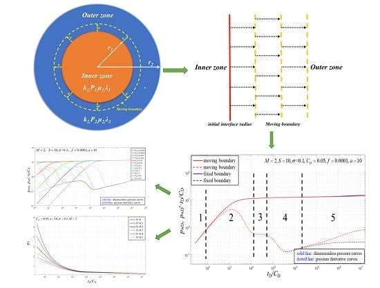
:The mathematical model of composite reservoir has been widely used in well test analysis. In the process of oil recovery, due to the injection or replacement of the displacement agent, the model boundary can be moved. At present, the mathematical model of a composite reservoir with a moving boundary is less frequently studied and cannot meet industrial demand. In this paper, a mathematical model of a composite reservoir with a moving boundary is developed, with consideration of wellbore storage and skin effects. The characteristics of pressure transient in moving boundary composite reservoir are studied, and the influences of parameters, such as initial boundary radius, moving boundary velocity, skin factor, wellbore storage coefficient, diffusion coefficient ratio, and mobility ratio on pressure and production, are analyzed. The moving boundary effects are noticeable mainly in the middle and late production stages. The proposed model provides a novel theoretical basis for well test analysis in these types of reservoirs.
1. Introduction
A composite reservoir model is widely used to model reservoirs with distinct regional properties variations. Among others, these variations may be caused by changes in formation physical properties, foreign fluids intrusion, and changes in formation fluid characteristics. These two different areas are separated by a discontinuous interface. Actual production cases often need to be modeled as a composite reservoir, such as in the cases of reservoir flooding (water, gas, chemical, steam) and formation stimulation. In addition, if the formation is stimulated or damaged, it can also be considered a composite reservoir. Therefore, the composite reservoir model has been widely investigated in literature [1,2,3,4,5,6,7,8,9,10,11]. However, there is very little research on composite reservoirs with a moving boundary. There are many cases in which a moving boundary is formed in the actual production process. For example, piston displacement or steam flooding may cause boundary movement. It can be seen that studying the moving boundary has far-reaching effects on the theory of composite reservoirs and industrial demand.
Current pressure transient analysis is an important method for analyzing reservoir characteristics. Most investigators only consider closed, constant pressure, and infinite acting boundaries in their composite reservoir models. These assumptions may lead to biased interpretation if moving boundaries do actually exist. Therefore, it is particularly important to analyze the transient pressure response of composite reservoir with moving boundary. Many papers and methods have been published on the flow of fluids in porous media [12,13,14,15,16,17,18], but the most common method used in petroleum engineering is still pressure-transient analysis.
Research activities on composite reservoir models were increasing in 1960s. Many models have been built and many methods have been applied to analyze the pressure characteristics of composite reservoir. Analytical solutions for media with the same center but different permeability have already appeared in the materials heat shrinkage literature published by Carslaw and Jaeger [19]. Subsequently, some research projects in the literature used composite reservoir models to study the pressure characteristics of reservoirs. In 1960, Hurst proposed a point-sink solution for infinitely large composite reservoirs and described many of the effects of oilfield disturbances involving fluid flow, volumetric behavior, and stratigraphic differences [20]. In 1961, Lucks and Guerrero studied the pressure characteristics of composite reservoir and calculated their pressure distribution. They compared the results with a uniform reservoir and found that the permeability and the size of the inner zone of the composite reservoir under certain conditions can be determined by the pressure drop curves [1]. In 1966, Carter proposed a method to describe the pressure behavior of a finite circular composite reservoir, and gave an analytical solution to the problem of micro-compressible fluid flow [2]. Other studies on pressure drop include Closmann and Ratliff [21], Bixel and Van Poollen [22], and Merrill et al. [23].
Among the research of the above scholars, the well test curves of composite reservoir are particularly important [24]. Scholars have done a lot of research on the effects of various factors on the well test curves. In 1985, Satman studied the interference problem in a composite reservoir and proposed a new solution to analyze the pressure response of composite reservoir observation wells, taking into account the effects of wellbore storage and skin [25]. Based on this, Olarewaju and Lee established an analytical model for the two-zone radial composite reservoir system and proposed a well test curves analysis method. Important parameters such as permeability and wellbore storage coefficient can be determined and production can be predicted [26]. Boussalem et al. studied the effect of mobility on pressure and pressure derivatives in closed composite reservoirs [27]. The influence of each parameter on the well test curve is significant, and the influence of different boundary conditions on the well test curve cannot be ignored. In 1996, Issaka summarized the analytical solutions for the pressure characteristics of composite reservoir under different flow geometries [28]. Then, Issaka and Ambashha proposed a new design equation related to the specific flow patterns observed in the test of spherical and linear composite reservoir, and studied the pressure derivative curves [29]. Based on the composite reservoir in the second zone, Ambastha et al. studied the pressure characteristics of the composite reservoir in the three zones and further improved the well testing theory of the composite reservoir [30].
Jordan and Mattar compared the pressure characteristics of composite reservoir with two-layer reservoirs [31]. They concluded that their stress characteristics are similar during transient flow, but if the model is not suitable, there will be large deviations at later production time. From this point of view, accurate model description is very important for transient pressure analysis. Scholars have established different mathematical models to characterize a wide variety of composite reservoirs. For composite reservoirs with faults, Rahman et al. proposed a model to describe the flow conditions of nearby wells [32]. Wang et al. used the method of sink source superposition and integral transformation to solve the solution of the new model of multiple permeability of composite reservoir, and studied the influence of different parameters and various boundaries on downhole pressure [33]. Imad et al. proposed a new model of horizontal well dual-porosity composite reservoir and studied its pressure characteristics [34]. Nie et al. proposed a new model of transient well test and diminution analysis of composite reservoir by using the effective radius method, and successfully eliminated the oscillation of the well test curves to solve the negative skin effect problem [35]. Wang et al. derived the nonlinear flow control equation of composite reservoir fluid based on Darcy’s law and material balance. The nonlinear N-zone model was established and solved, and different well test curves were drawn taking into account the quadratic gradient term [36]. Zhang et al. used the constructor method to derive the continuous point source function of the composite reservoir under three kinds of boundaries, analyzed the pressure characteristics, and plotted the well test curves [6]. Gu et al. proposed a two-hole fractal fractional diffusion model for composite reservoir [37]. Olarewaju et al. established an analytical model for composite reservoirs produced at constant bottom hole pressure or constant rate [38]. The above research has played an important role in the development of well testing theory in composite reservoirs.
At present, a well testing theory has been developed, and the mathematical models of composite reservoir are also very mature, but the analysis of pressure transients and transient production of composite reservoir with moving boundary remains understudied [39]. Khatib and Noaman proposed a mathematical model to describe transient pressure behavior in composite reservoir-aquifer system [40]. They used the finite difference method to solve equations in Laplace space and estimated the position of the moving front using an iterative procedure. However, the accuracy of the solutions obtained by the finite difference method is lower than the precision of the analytical solution, and they do not consider the influence of the initial interface radius and the diffusion coefficient ratio on the pressure and production. These aspects also require more in-depth research. The purpose of this paper is to study the pressure and production characteristics of composite reservoir with moving boundary. First, we used a mathematical model to accurately characterize composite reservoir, including governing equations, initial conditions, and boundary conditions. Second, in order to study the influence of various reservoir parameters on pressure and production, we carried out parameter sensitivity analysis and summarized its influence law. Based on the Darcy’s Law, we established a mathematical model. We transformed the model into Laplace space [41], and found that the transformed model is a Bessel function [42]. Therefore, we obtained the analytical solution of the transformed model. Compared with previous studies, the accuracy of our model’s solution is higher [40]. The Stehfest algorithm is then used to invert the value of the solution into real-time space [43]. This paper consists of five parts, arranged as follows: Section 1 is the introduction part, which briefly introduces the research content, analyzes the literature related to this research, and summarizes the previous research results in this field. Section 2 is the description part of the model and introduces the basis for building mathematical model, which is based on the Darcy’s Law. Section 3 is the solution part of the model. Section 4 discusses the results of the second and third sections, mainly analyzing the pressure characteristics and the influence of various factors on pressure and output. Section 5 summarizes this paper based on research content.
2. Model Description
2.1. Physical Model and Assumptions
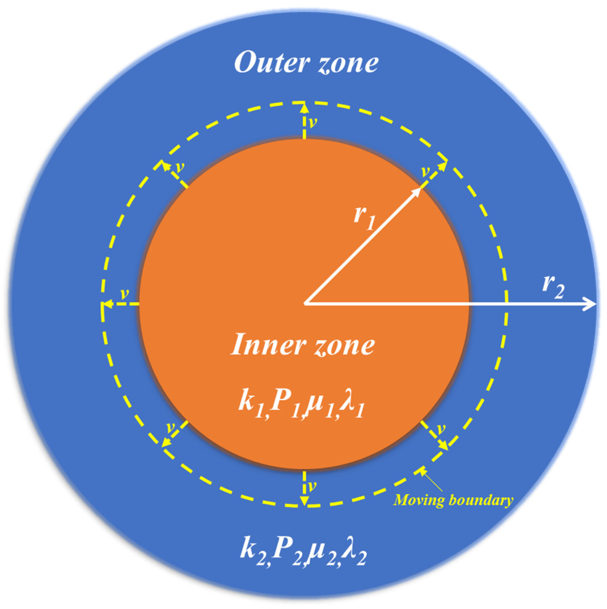
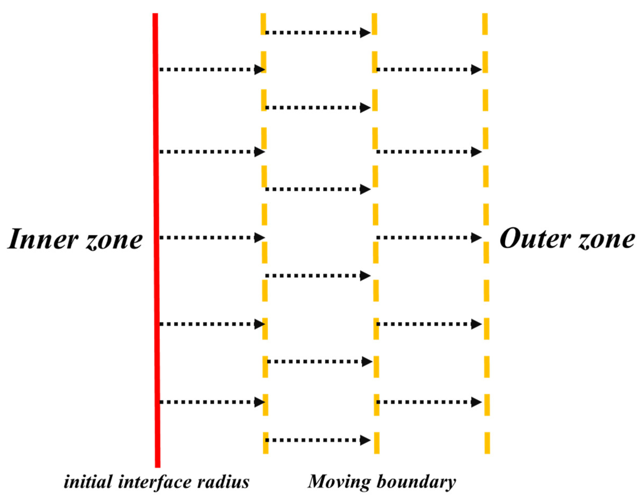
Moving boundary composite reservoir means that the radius of the composite reservoir interface may move under certain conditions. Figure 1 is a schematic diagram of the moving boundary composite reservoir, and Figure 2 is a schematic diagram of boundary movement. It can be seen from Figure 1 that the composite reservoir is divided into two areas: the inner zone (indicated by 1) and the outer zone (indicated by 2). It is assumed here in that the interface between the inner and outer zones is a moving boundary that moves outward at a certain speed, as shown in Figure 2. Based on the fixed boundary, the well test interpretation model of the moving boundary composite reservoir was established, and the numerical solution of the model was obtained. At the same time, the parameter sensitivity analysis was carried out to obtain the influence of each important parameter on the well test curves.
The following assumptions were made before establishing a well test interpretation model for a moving boundary composite reservoir:
- (1)
- The reservoir is homogeneous, horizontal, uniform in thickness, and isotropic;
- (2)
- The original formation pressure (indicated by Pi) is evenly distributed, and the production rate of well is fixed after the well is opened;
- (3)
- The formation rocks and fluids are all slightly compressible;
- (4)
- The formation fluid conforms to the Darcy seepage law during seepage;
- (5)
- Wellbore storage and skin effects are accounted;
- (6)
- Gravity and capillary forces are ignored;
- (7)
- At the interface between the inner and outer zones, there is no flow loss and the formation pressure is not abrupt, and the interface moves with the propagation of mass wave;
- (8)
- The outer boundary condition is an infinite outer boundary;
- (9)
- The inner boundary expands to the outer region over time.
2.2. Factor Decomposition Model
2.2.1. Dimensionless Variables Definition
In order to make the equation easy to solve, the following dimensionless variables are defined:
where is the dimensionless pressure; i = 1,2 (when i = 1, it denotes moving boundary composite reservoir inner zone; when i = 2, it denotes moving boundary composite reservoir outer zone); is dimensionless time; is the dimensionless radius of the formation centered on the well. is the dimensionless inner radius; is the dimensionless wellbore storage factor; is the inner zone permeability (unit:); h is the oil layer thickness (unit: m); is the original formation pressure (unit: MPa); is the pressure at a certain point in the formation(unit: MPa); is ground flow (unit:); is fluid viscosity (unit: ); B is the volume factor (unit:); is porosity; is the total system compressibility (unit:); is the wellbore radius (unit: m); r is the distance from the center of the well (unit: m); is the inner radius (unit: m); S is the skin factor (dimensionless).
2.2.2. Governing Equations
Based on the above nine assumptions combined with the general three-dimensional seepage differential equation, the dimensionless well test model of the composite boundary reservoir can be obtained:
Comprehensive differential equations are shown in Equations (5)–(6):
Inner area:
Outer area:
where denotes the diffusion coefficient ratio, dimensionless.
2.2.3. Initial and Boundary Conditions
Initial conditions, internal boundary conditions and interface conditions of the dimensionless well test model of the composite boundary reservoir are shown as following:
Initial conditions:
Internal boundary conditions:
Interface conditions:
where denotes outer zone mobility ratio and denotes mobility.
If it is an infinite outer boundary, Equation (11) can be obtained as follows:
3. Model Solution
Performing a Laplace transform on the Equations (5)–(11) to obtain the following formula: Comprehensive differential equations are shown in Equations (12)–(13).
Inner area:
where and are image functions in a pull space and z is the Laplace parameter.
Outer area:
Initial conditions:
Internal boundary conditions:
Interface conditions:
Outer boundary conditions:
The governing equations (Equations (12)–(13)) are the Bessel-type ordinary differential equations, and the general solution of Equations (12)–(13) are solved as follows:
where A,B,C,D are the coefficient; , are the first type of virtual zero-order and first-order Bessel functions; , are the second type of virtual zero-order and first-order Bessel functions.
In Equation (20), when , there must be C = 0, thus:
Bringing Equation (19) and Equation (21) into Equations (15)–(17) produces:
Let , , , , , , , .
The coefficients obtained by solving Equations (22)–(24) are as follows:
Thus, the bottom hole pressure solution is expressed in Equation (28) as follows:
where is the dimensionless downhole pressure solution without considering the influence of wellbore storage and skin effects under pull space.
Then, introducing the wellbore storage and skin effects and applying the Duhamel’s principle, the downhole pressure solution considering the influence of wellbore storage and skin effects is shown in Equation (29):
where is the dimensionless downhole pressure solution considering the influence of wellbore storage and skin effects under pull space.
Assuming t = 0, , when t = 0, it is assumed that the interface moves with the propagation of the mass wave and satisfies , where c is the coefficient, c = 1 when the piston is displaced, and c is the water rising rate when the piston is not displaced. Before the mass wave reaches the boundary, the interface position does not change. After the mass wave reaches the boundary, the interface begins to move. Suppose that at a certain moment , the mass wave reaches the boundary (where is affected by the parameters of the formation, and the value can be analyzed), the following formula can be obtained:
When:
When:
where a is initial interface radius (unit: m); Q is production (unit: ); t is production time (unit: d); is the propagation time of the mass wave at the interface (unit: d).
When time is turned into a dimensionless form Equation (32) is obtained:
Equations (30)–(31) are transformed into dimensionless form, and Equations (33)–(34) are obtained:
Let ) and define f as the moving speed of the moving boundary, then, the following formula can be obtained:
According to the actual production situation of the oil field, the value of f in Equation (35) can be analyzed.
According to the definition of dimensionless variables, the relationship between dimensionless production at the bottom hole pressure and the dimensionless bottom hole flow at constant production can be derived:
where is the dimensionless production at the bottom hole pressure under the pull space.
The dimensionless production at the bottom of the well can be obtained from Equation (36). The Stehfest numerical inversion method is used to obtain a solution for the true space production, and the parameter sensitivity analysis is performed by MATLAB programming (MATLAB R2017b, MathWorks, America).
4. Results Analysis and Discussion
4.1. Flow Regimes Analysis
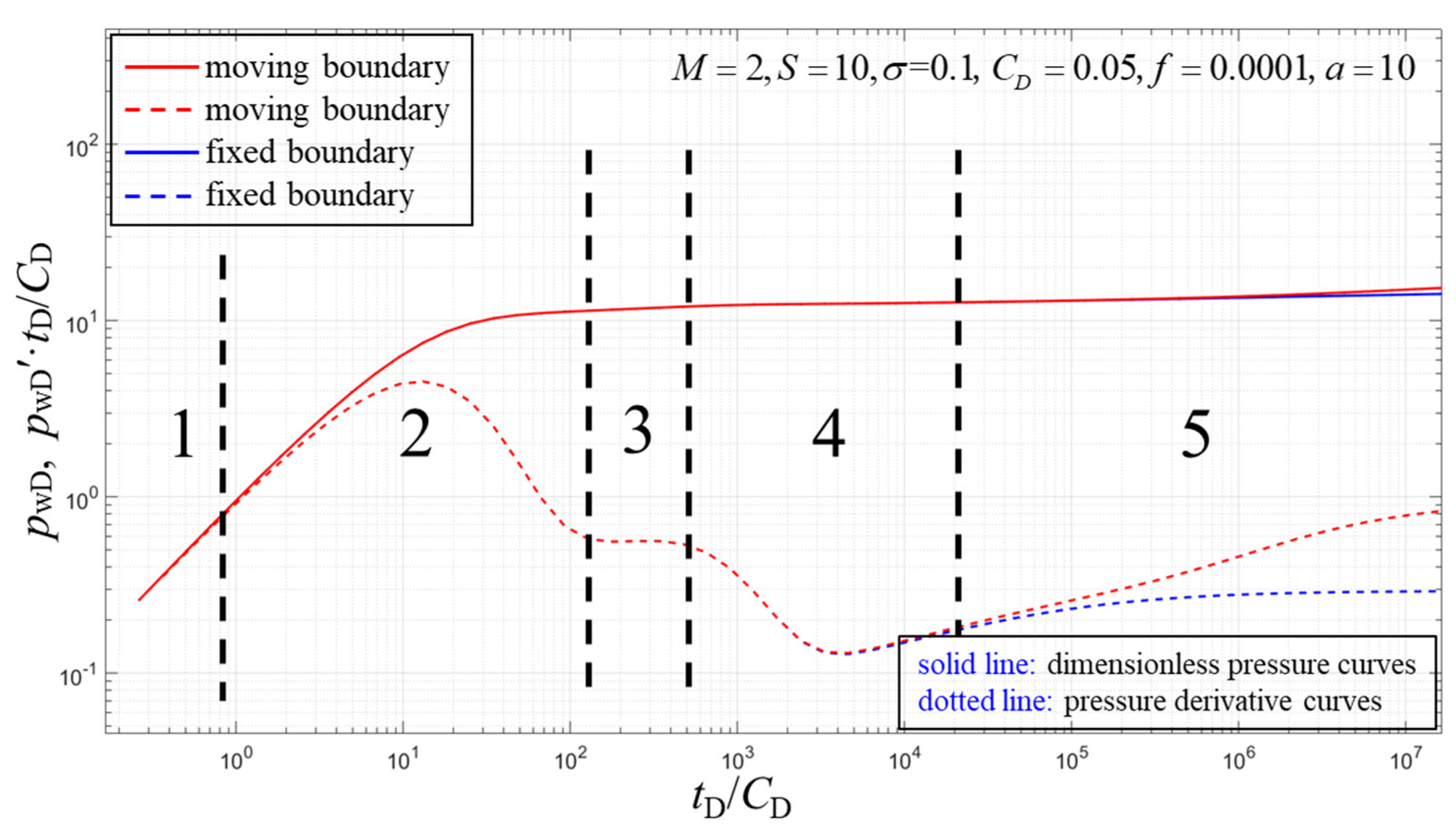
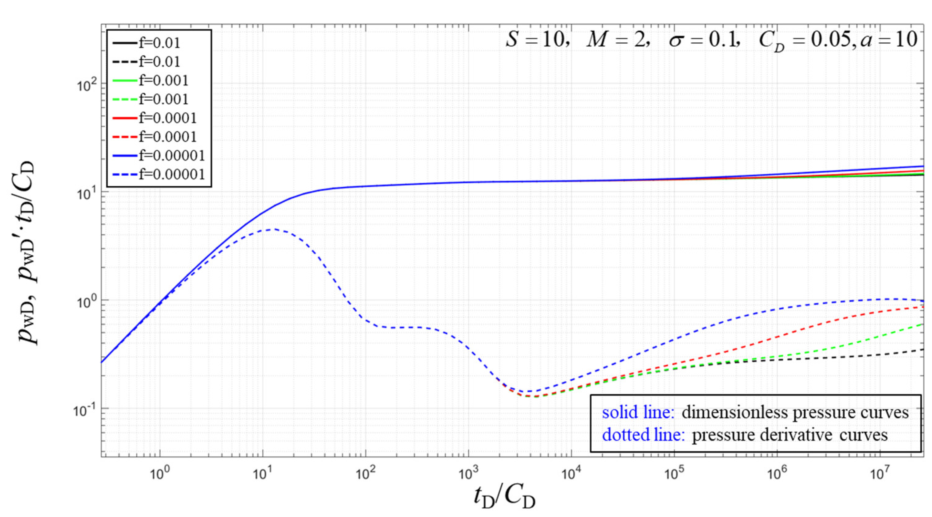
It can be seen from Figure 3 that the dimensionless pressure curves (solid line) and the derivative curves (dashed line) of the moving boundary composite reservoir can be divided into five flow states.
The first stage is the pure wellbore storage flow period, which appears as a straight line with a slope of 1.
The second stage is the transition period of the pure wellbore storage flow to the inner zone radial flow. The skin and wellbore storage coefficients affect the duration of the phase and the height of the peak.
The third stage is the inner zone radial flow period. This stage is affected by the interface radius between the inner and outer zones.
The fourth stage is the transition period of the radial flow of the inner zone to the radial flow of the moving boundary.
The last stage is the radial flow period of the moving boundary. Since the boundary is always moving, the derivative curves are not a horizontal line but an upturned curve. This stage can be approximated as a radial flow, and the movement of the boundary affects it.
4.2. Pressure Parameter Sensitivity Analysis
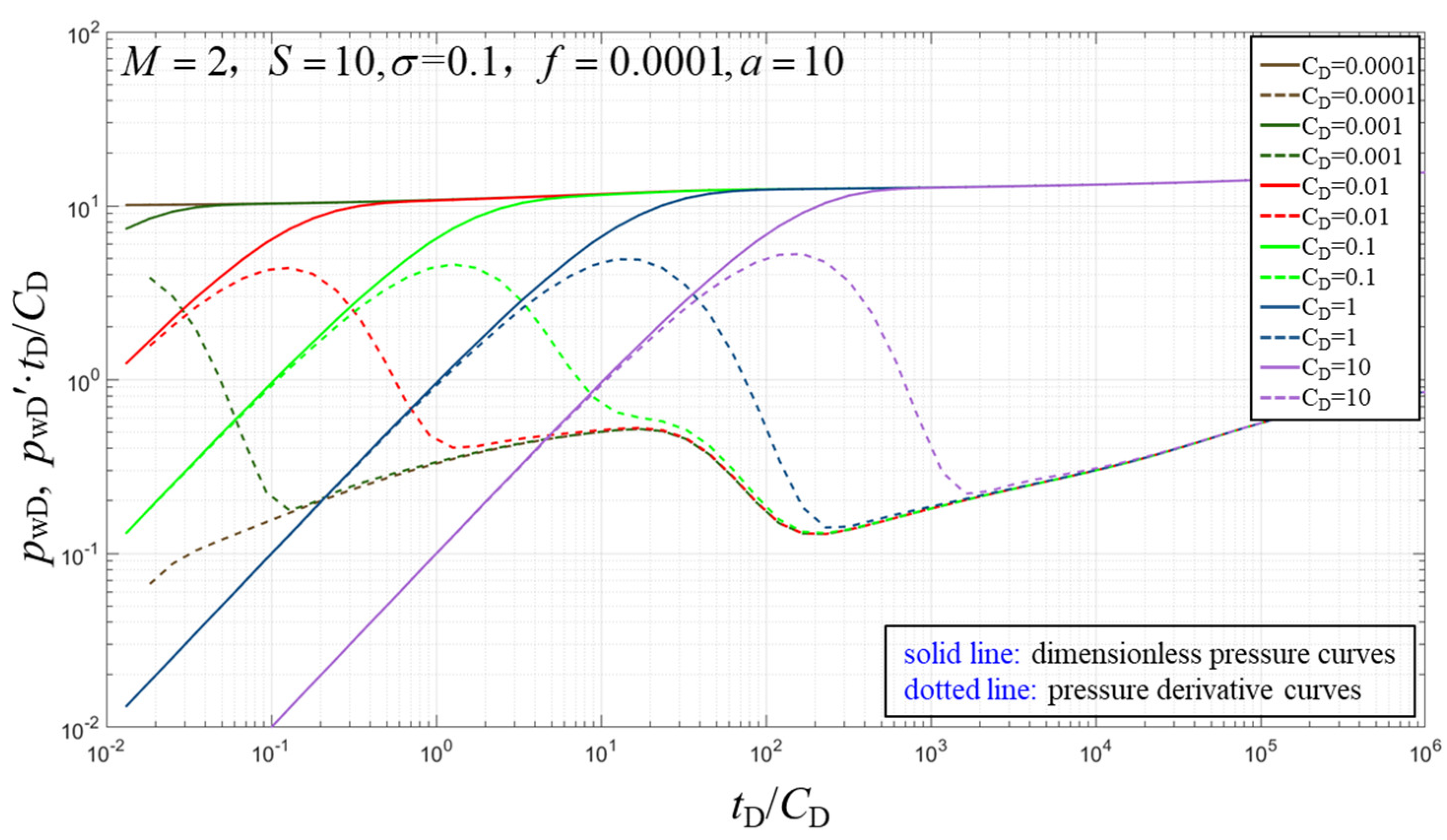
4.2.1. Effect of Wellbore Storage
As shown in Figure 4, the larger the value of , the longer the duration of the pure wellbore storage phase, which appears as a shift in the pressure and pressure derivative curves to the right. This is because when the value of is large, the inner zone is greatly affected by the wellbore storage effect, and the radial flow phase is delayed. When the wellbore storage coefficient is relatively large (), the inner zone radial flow period and transition flow period will disappear. Conversely, the smaller the value of , the less affected the inner zone is by the wellbore storage. The time to reach the radial flow period of the inner zone is shortened, and the radial flow period of the inner zone is prolonged. When the mass wave propagates to the moving boundary, the influence of the wellbore storage effect will disappear, thus, the pressure derivative curves of the infinite radial flow period in the later outer zone will tend to be consistent.
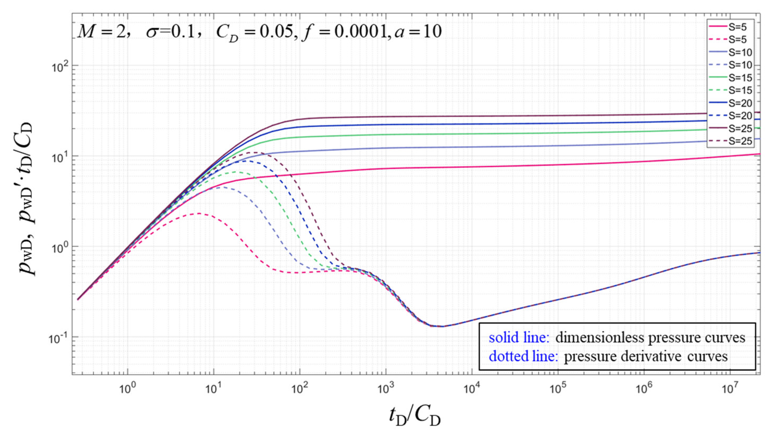
4.2.2. Effect of Skin Factor
As shown in Figure 5, the larger the value of S, the larger the peak of the pressure and pressure derivative curves. Conversely, the smaller the value of S, the smaller the peak of the pressure and pressure derivative curves. This is due to the stimulation and formation damage, which has caused the permeability of the formation in the near-well zone to change, thus, creating additional resistance. The larger the skin factor, the greater the additional resistance generated; thus, the pressure drop in the near-well zone is greater, and the larger the opening is on the curves. Similarly, if the skin factor is too large and the inner zone radius is small, the inner zone radial flow period may also disappear. Since the skin factor only affects the near-well zone, the flow state of the fluid during the transition period and the radial flow period of the moving boundary is not affected, and the pressure derivative curves coincide at these stages.
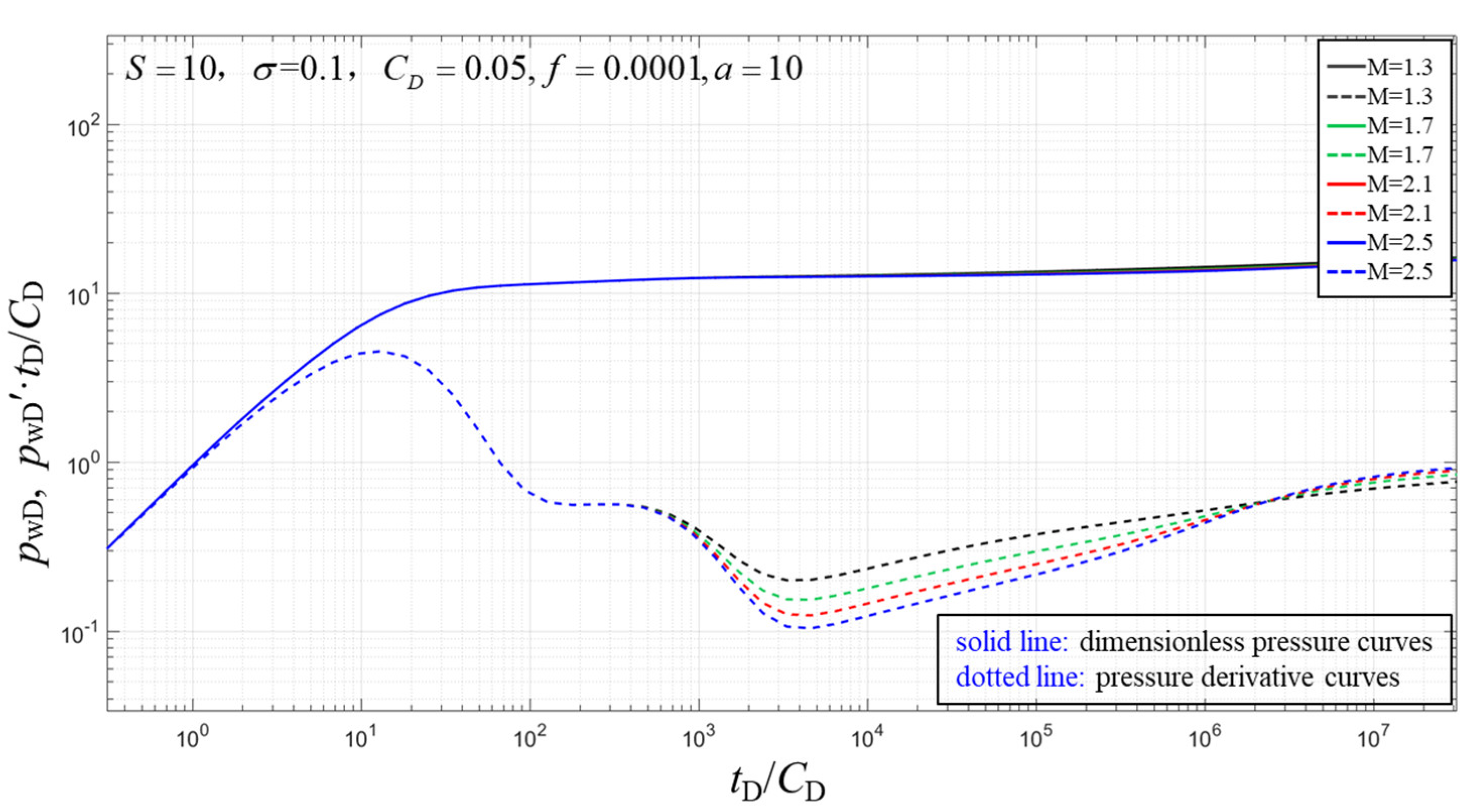
4.2.3. Effect of Mobility Ratio
As shown in Figure 6, the pressure curves will be upturned in the radial flow period of the moving boundary. If the mobility of the inner zone is larger than the outer zone, then the fourth stage (transition period) will tilt down. On the other hand, if the inner zone’s mobility is smaller than the outer zone, the fourth stage will be lifted upward. The closer the mobility ratio value is to one, the smoother the transition phase of the curve. This is because the closer the mobility ratio is to one, the smaller the difference between the inner and outer zones, and the shorter the duration of the transition phase. The larger the value of M, the larger the upturn. This is because the greater the mobility ratio, the longer the duration of the transition phase, the more obvious the effect of the moving boundary, and the larger the upturn on the curves.
4.2.4. Effect of Diffusion Coefficient
As shown in Figure 7, mainly affects the transition phase of the radial flow from the inner zone to the radial flow of the moving boundary. The larger the value of , the more gentle the pressure derivative curves. The smaller the value of , the more obvious the "concave" produced during the transition phase. The main reason is that when the fluid ratio in the inner and outer zone and the viscosity of the reservoir fluid are constant, the larger the value of , the faster the mass wave propagates and spreads at the interface, and the curves shows that the pressure derivative curves is gentler. When the mass wave propagates to the moving boundary, the above influence will gradually disappear, thus, the pressure derivative curves of the infinite radial flow stage in the outer zone will be more consistent again in the later stage of development.
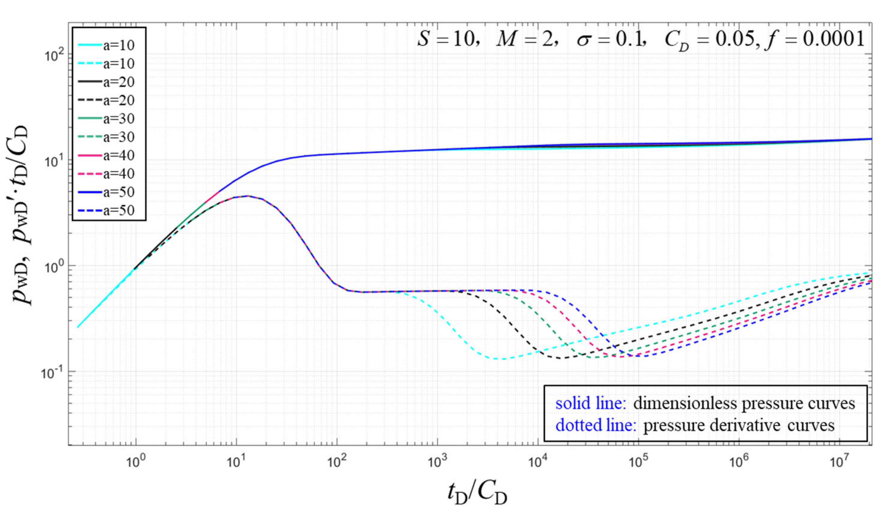
4.2.5. Effect of Initial Interface Radius
As shown in Figure 8, as the radius of the interface becomes larger, the transition from the radial flow of the inner zone to the radial flow of the moving boundary on the pressure derivative curves moves to the right. This shows that the duration of the radial flow phase of the inner zone becomes longer, and the time during which the mass wave propagates to the outer zone is also delayed. If the interface radius between the inner and outer regions is relatively large, the fluid in the inner region will gradually enter the radial flow period, where the derivative value is 0.5 in the dimensionless coordinates. At this point, the straight line segment will appear on the single logarithmic plot. However, if the radius at the interface between the inner and outer regions is relatively small, the radial flow period of the fluid may disappear and it will go directly to the fourth stage.
4.2.6. Effect of Moving Boundary Moving Speed
As shown in Figure 9, as the value of f increases, the duration of the radial flow period of the moving boundary becomes longer. Therefore, the influence of the production boundary in the middle and late time production is greater. However, when the moving speed of the moving boundary is low, the pressure derivative curve becomes smoother in advance. The influence caused by the moving boundary disappears quickly. It can be seen from Figure 3 that the pressure derivative curves of the moving boundary and the fixed boundary differ greatly in the middle and late time of production. Affected by the boundary, the pressure derivative and the pressure curves rise. It can be seen that the moving boundary causes pressure loss, which is not conducive to production.
4.3. Transient Production Parameter Sensitivity Analysis
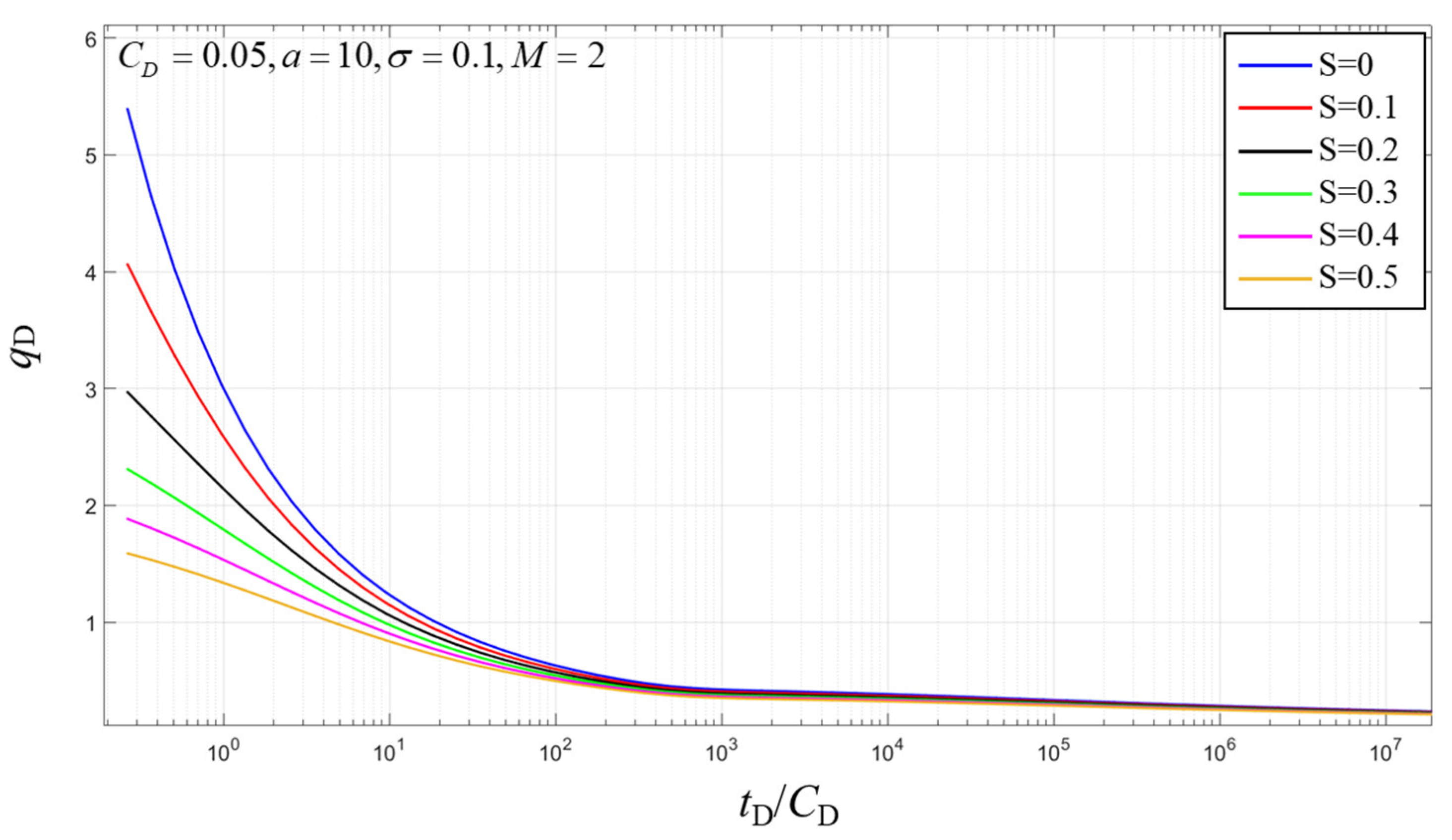
4.3.1. Effect of Skin Factor
As can be seen from Figure 10, the effect of the skin factor on the production is relatively large at the initial stage. The production at the initial moment decreases as the skin factor increases. However, after a long period of production, the effect of the skin on production will become smaller and smaller until it disappears. A large S value represents a reduction of the permeability in the near-well bore zone, or formation damage. For example, the blockage caused by the migration of rock particles in the reservoir or the incompatibility of the drilling fluid and the formation fluid makes the seepage resistance in the near-well zone become larger and the wells’ production becomes lower. The implementation of stimulation measures will reduce the seepage resistance of the near-well belt, that is, S becomes smaller or even becomes a negative number with large absolute values, and the production will also increase significantly.
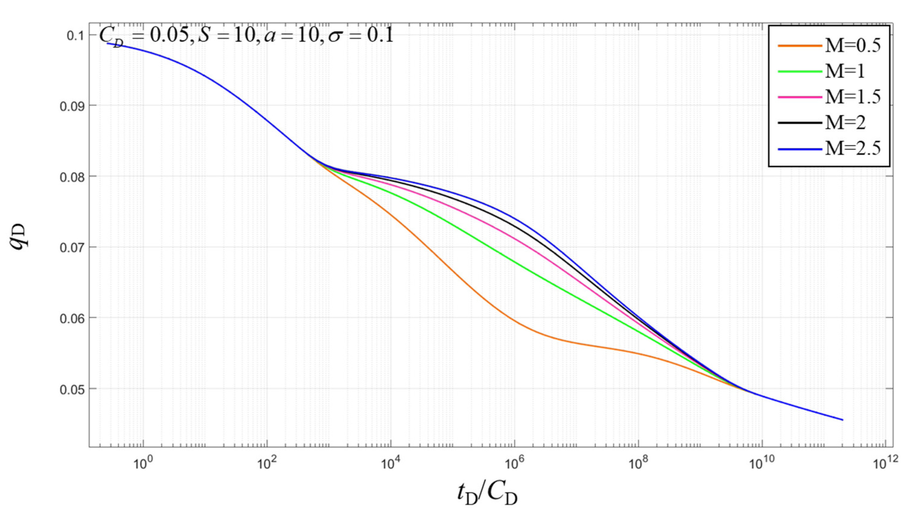
4.3.2. Effect of Mobility Ratio
As can be seen from Figure 11, when M = 1, the rate of decline in production is constant, because the formation is not damaged or stimulated. When M>1, the mobility in the outer region becomes higher, the pressure drop becomes smaller, and the rate of decline in production becomes slower. When M < 1, the mobility in the outer region becomes lower, the pressure drop becomes larger, and the rate of decline in production becomes faster. In addition, it can be concluded from Figure 11 that in the final stage, the effect of the internal regional properties on production is gradually reduced until it disappears.
4.3.3. Effect of Diffusion Coefficient
As shown in Figure 12, the value of has little effect on the early production decline curves. After a certain period of production, as becomes larger, the rate of decline in production becomes faster, because the faster the diffusion rate, the greater the pressure drop. Moreover, in the fluid to infinity, the influence of the internal area gradually disappears.
4.3.4. Effect of Initial Interface Radius
As can be seen from Figure 13, the value of a has little effect on production in the early stage. However, as the production time becomes longer, the influence of a on production gradually increases. This is related to the ratio of mobility in the inner and outer zones. If the mobility of the inner region is smaller than the mobility of the outer region, as the value of a becomes larger, the rate of decrease in production is faster. Because the mobility of the inner zone is small, the pressure drop is large. Therefore, as the value of a becomes larger, the rate of production decrease becomes faster. In the final stage, the influence of physical parameters such as skin factor and mobility ratio on production gradually disappeared.
5. Conclusions
In this paper, the seepage mechanism of the moving boundary composite reservoir and the solution method of the well test model are studied. A well test interpretation model for moving boundary composite reservoirs was established and the model was solved. Then, the pressure, pressure derivative, and production characteristic curve were plotted. Finally, the parameter sensitivity analysis is carried out, and the following conclusions are drawn::
- (1)
- The composite reservoir consists mainly of two zones: the inner zone and the outer zone. The pressure and pressure derivative curves include a total of five flow stages, including pure wellbore storage flow period, transition period of the pure wellbore storage flow to the inner zone radial flow, inner zone radial flow period, transition period of the radial flow of the inner zone to the radial flow of the moving boundary, and radial flow period of the moving boundary.
- (2)
- The wellbore storage coefficient increases, and the duration of the pure wellbore storage phase also increases. The larger the skin factor, the higher the peak of the pure wellbore storage flow to the inner zone radial flow transition phase. The greater the mobility ratio in the inner and outer zones, the higher the radial flow phase in the outer zone and the higher the upturn in the radial flow section of the moving boundary. The smaller the diffusion coefficient, the deeper the “concave” of the inner zone radial flow to the outer zone radial flow transition phase. The larger the initial interface radius, the longer the inner radial flow segment lasts. As the moving speed of the boundary increases, the duration of the radial flow period of the moving boundary becomes longer. Affected by the boundary, the pressure derivative and the pressure curves rise. It can be seen that the moving boundary causes pressure loss, which is not conducive to production.
- (3)
- For composite reservoir with moving boundary, as the skin factor increases, the initial production gets lower and lower. As the ratio of internal and external flow increases, the rate of decline is faster. The diffusion coefficient has little effect on the early production decline curves, but after a certain period of production, the production decreases rapidly as the diffusion coefficient increases. The interface radius has little effect on early production, but its influence increases as production time increases. If the mobility of the inner zone is greater than the mobility of the outer zone, the production decreases as the radius becomes larger, whereas the production increases as the radius becomes larger.
Author Contributions
Z.S., X.Y. and Y.J. and conceived and designed the numerical investigation; Z.S., X.Y. and S.S. created the numerical model; X.Y. and M.W. summarized the thermal recovery evaluation system; X.Y. and S.S. examined the accuracy of the proposed model; M.W. and X.Y. analyzed the result; Z.S. and X.Y. contributed analysis tools; X.Y. and Y.J. wrote the manuscript; Z.S., X.Y. and Y.J. make a great contribution to the revision of manuscript. All authors have read and agreed to the published version of the manuscript.
Funding
This study was supported by the National Natural Science Foundation of China (Grant No. 51774317), the Fundamental Research Fund for Central Universities (Grant No. 18CX02100A) and and National Science and Technology Major Project (Grant NO.2016ZX05011004-004).
Acknowledgments
This study was jointly supported by the National Natural Science Foundation of China (Grant NO.51774317), the Fundamental Research Funds for the Central Universities (Grant No.18CX02100A) and National Science and Technology Major Project (Grant NO.2016ZX05011004-004). We are grateful to all staff involved in this project, and also wish to thank the journal editors and the reviewers whose constructive comments improved the quality of this paper greatly.
Conflicts of Interest
The authors declare that they have no conflict of interest.
Nomenclature
| pressure at a certain point in the formation, MPa | |
| ground flow, | |
| fluid viscosity, | |
| inner zone permeability, | |
| B | volume factor, |
| porosity, fraction | |
| wellbore radius, m | |
| r | distance from the left of the well, m |
| inner radius, m | |
| S | skin factor, fraction |
| h | oil layer thickness, m |
| original formation pressure, MPa | |
| a | initial interface radius, m |
| Q | production, |
| t | production time, d |
| diffusion coefficient ratio, fraction | |
| M | outer zone mobility ratio, fraction |
| A,B,C,D | coefficient, fraction |
| c | coefficient, fraction |
| total system compressibility, | |
| propagation time of the mass wave at the interface, d | |
| f | moving speed of the moving boundary |
| dimensionless production | |
| dimensionless pressure | |
| dimensionless time | |
| dimensionless radius | |
| dimensionless inner radius | |
| CD | dimensionless wellbore storage factor |
| dimensionless downhole pressure solution | |
| , | first type of virtual zero-order and first-order Bessel functions |
| , | second type of virtual zero-order and first-order Bessel functions |
| Dim. pressure | dimensionless pressure |
Subscript
| D | dimensionless |
Superscript
| Laplace transform |
References
- Loucks, T.; Guerrero, E. Pressure drop in a composite reservoir. Soc. Pet. Eng. J. 1961, 1, 170–176. [Google Scholar] [CrossRef]
- Carter, R. Pressure behavior of a limited circular composite reservoir. Soc. Pet. Eng. J. 1966, 6, 328–334. [Google Scholar] [CrossRef] [Green Version]
- Ambastha, A.; McLeroy, P.; Grader, A. Effects of a partially communicating fault in a composite reservoir on transient pressure testing. SPE Form. Eval. 1989, 4, 210–218. [Google Scholar] [CrossRef]
- Chu, W.-C.; Shank, G.D. A new model for a fractured well in a radial, composite reservoir (includes associated papers 27919, 28665 and 29212). SPE Form. Eval. 1993, 8, 225–232. [Google Scholar] [CrossRef]
- Escobar, F.-H.; Martínez, J.-A.; Montealegre-Madero, M. Pressure and pressure derivate analysis for a well in a radial composite reservoir with a non-newtonian/newtonian interface. Ct F Cienc. Tecnol. Y Futuro 2010, 4, 33–42. [Google Scholar]
- Zhang, L.-H.; Zhao, Y.; Liu, Q. Well-test-analysis and applications of source functions in a bi-zonal composite gas reservoir. Pet. Sci. Technol. 2014, 32, 965–973. [Google Scholar] [CrossRef]
- Liu, Q.; Lu, H.; Li, L.; Mu, A. Study on characteristics of well-test type curves for composite reservoir with sealing faults. Petroleum 2018, 4, 309–317. [Google Scholar] [CrossRef]
- Razminia, K.; Razminia, A.; Trujilo, J.J. Analysis of radial composite systems based on fractal theory and fractional calculus. Signal Process. 2015, 107, 378–388. [Google Scholar] [CrossRef]
- Meng, F.; Lei, Q.; He, D.; Yan, H.; Jia, A.; Deng, H.; Xu, W. Production performance analysis for deviated wells in composite carbonate gas reservoirs. J. Nat. Gas Sci. Eng. 2018, 56, 333–343. [Google Scholar] [CrossRef]
- Wu, M.; Ding, M.; Yao, J.; Li, C.; Huang, Z.; Xu, S. Production-Performance Analysis of Composite Shale-Gas Reservoirs by the Boundary-Element Method. SPE Reserv. Eval. Eng. 2018, 22. [Google Scholar] [CrossRef] [Green Version]
- Wu, M.; Ding, M.; Yao, J.; Xu, S.; Li, L.; Li, X. Pressure transient analysis of multiple fractured horizontal well in composite shale gas reservoirs by boundary element method. J. Pet. Sci. Eng. 2018, 162, 84–101. [Google Scholar] [CrossRef]
- Gringarten, A.C.; Ramey, H.J., Jr. The use of source and Green’s functions in solving unsteady-flow problems in reservoirs. Soc. Pet. Eng. J. 1973, 13, 285–296. [Google Scholar] [CrossRef]
- Ozkan, E.; Raghavan, R. Some New Solutions to Solve Problems in Well Test Analysis: Part 2—Computational Considerations and Applications; Society of Petroleum Engineers: Richardson, TX, USA, 1988; pp. 1–67. [Google Scholar]
- Cheng, C.; Chau, K.; Sun, Y.; Lin, J. Long-term prediction of discharges in Manwan Reservoir using artificial neural network models. In International Symposium on Neural Networks; Springer: Berlin, Germany, 2005; Volume 3498, pp. 1040–1045. [Google Scholar]
- Chen, W.; Chau, K. Intelligent manipulation and calibration of parameters for hydrological models. Int. J. Eniron. Pollut. 2006, 28, 432–447. [Google Scholar] [CrossRef] [Green Version]
- Chau, K.-W. An ontology-based knowledge management system for flow and water quality modeling. Adv. Eng. Softw. 2007, 38, 172–181. [Google Scholar] [CrossRef] [Green Version]
- Taormina, R.; Chau, K.-W.; Sethi, R. Artificial neural network simulation of hourly groundwater levels in a coastal aquifer system of the Venice lagoon. Eng. Appl. Artif. Intell. 2012, 25, 1670–1676. [Google Scholar] [CrossRef] [Green Version]
- Mohebbi, R.; Delouei, A.A.; Jamali, A.; Izadi, M.; Mohamad, A.A. Pore-scale simulation of non-Newtonian power-law fluid flow and forced convection in partially porous media: Thermal lattice Boltzmann method. Phys. A Stat. Mech. Appl. 2019, 525, 642–656. [Google Scholar] [CrossRef]
- Carslaw, H.S.; Jaeger, J.C. Conduction of Heat in Solids, 2nd ed.; Clarendon Press: Oxford, UK, 1959. [Google Scholar]
- Hurst, W. Interference between Oil Fields; Society of Petroleum Engineers: Richardson, TX, USA, 1960; Volume 219, pp. 175–192. [Google Scholar]
- Closmann, P.; Ratliff, N. Calculation of transient oil production in a radial composite reservoir. Soc. Pet. Eng. J. 1967, 7, 355–358. [Google Scholar] [CrossRef]
- Bixel, H.; van Poollen, H. Pressure drawdown and buildup in the presence of radial discontinuities. Soc. Pet. Eng. J. 1967, 7, 301–309. [Google Scholar] [CrossRef]
- Merrill, L., Jr.; Kazemi, H.; Gogarty, W.B. Pressure falloff analysis in reservoirs with fluid banks. J. Pet. Technol. 1974, 26, 809–818. [Google Scholar] [CrossRef]
- Ambastha, A. Practical Aspects of Well Test Analysis under composite reservoir situations. J. Can. Pet. Technol. 1995, 34. [Google Scholar] [CrossRef]
- Satman, A. An analytical study of interference in composite reservoirs. Soc. Pet. Eng. J. 1985, 25, 281–290. [Google Scholar] [CrossRef]
- Olarewaju, J.; Lee, W.J. A comprehensive application of a composite reservoir model to pressure transient analysis. In Proceedings of the SPE California Regional Meeting, Ventura, CA, USA, 8–10 April 1987; Society of Petroleum Engineers: Richardson, TX, USA, 1987; pp. 1–17. [Google Scholar]
- Boussalem, R.; Djebbar, T.; Escobar, F.H. Effect of mobility ratio on the pressure and pressure derivative of wells in closed composite reservoirs. In Proceedings of the SPE western regional/AAPG pacific section joint meeting, Anchorage, AK, USA, 20–22 May 2002; Society of Petroleum Engineers: Richardson, TX, USA, 2002; pp. 1–6. [Google Scholar]
- Issaka, M.B. Well Test Analysis for Composite Reservoirs in Various Flow Geometries. Ph.D. Thesis, University of Alberta, Edmonton, AB, Canada, 1996; pp. 1–128. [Google Scholar]
- Issaka, M.; Ambastha, A. A generalized pressure derivative analysis for composite reservoirs. J. Can. Pet. Technol. 1999, 38. [Google Scholar] [CrossRef]
- Ambastha, A.; Ramey, H., Jr. Pressure transient analysis for a three-region composite reservoir. In Proceedings of the SPE Rocky Mountain Regional Meeting, Casper, WY, USA, 18–21 May 1992; Society of Petroleum Engineers: Richardson, TX, USA, 1992; pp. 1–10. [Google Scholar]
- Jordan, C.; Mattar, L. Comparison of pressure transient behaviour of composite and two-layered reservoirs. J. Can. Pet. Technol. 2002, 41. [Google Scholar] [CrossRef]
- Rahman, N.; Miller, M.D.; Mattar, L. Analytical solution to the transient-flow problems for a well located near a finite-conductivity fault in composite reservoirs. In Proceedings of the SPE Annual Technical Conference and Exhibition, Denver, CO, USA, 5–8 October 2003; Society of Petroleum Engineers: Richardson, TX, USA, 2003; pp. 1–13. [Google Scholar]
- Wang, X.-D.; Zhou, Y.-F.; Luo, W.-J. A study on transient fluid flow of horizontal wells in dual-permeability media. J. Hydrodyn. 2010, 22, 44–50. [Google Scholar] [CrossRef]
- Brohi, I.G.; Pooladi-Darvish, M.; Aguilera, R. Modeling fractured horizontal wells as dual porosity composite reservoirs-application to tight gas, shale gas and tight oil cases. In Proceedings of the SPE Western North American Region Meeting, Anchorage, AK, USA, 7–11 May 2011; Society of Petroleum Engineers: Richardson, TX, USA, 2011; pp. 1–22. [Google Scholar]
- Nie, R.-S.; Guo, J.; Jia, Y.; Zhu, S.; Rao, Z.; Zhang, C. New modelling of transient well test and rate decline analysis for a horizontal well in a multiple-zone reservoir. J. Geophys. Eng. 2011, 8, 464–476. [Google Scholar] [CrossRef]
- Wang, X.-L.; Fan, X.; He, Y.; Nie, R.; Huang, Q. A nonlinear model for fluid flow in a multiple-zone composite reservoir including the quadratic gradient term. J. Geophys. Eng. 2013, 10, 045009. [Google Scholar] [CrossRef]
- Gu, D.; Ding, D.; Gao, Z.; Tian, L.; Liu, L.; Xiao, C. A fractally fractional diffusion model of composite dual-porosity for multiple fractured horizontal wells with stimulated reservoir volume in tight gas reservoirs. J. Pet. Sci. Eng. 2019, 173, 53–68. [Google Scholar] [CrossRef]
- Olarewaju, J.; Lee, W. An analytical model for composite reservoirs produced at either constant bottomhole pressure or constant rate. In Proceedings of the SPE Annual Technical Conference and Exhibition, Dallas, TX, USA, 27–30 September 1987; Society of Petroleum Engineers: Richardson, TX, USA, 1987; pp. 1–14. [Google Scholar]
- Wang, H.; Zhang, L. A boundary element method applied to pressure transient analysis of geometrically complex gas reservoirs. In Proceedings of the Latin American and Caribbean Petroleum Engineering Conference, Cartagena, Colombia, 31 May–3 June 2009; Society of Petroleum Engineers: Richardson, TX, USA, 2009; pp. 1–12. [Google Scholar]
- El-Khatib, N.A. Transient pressure behavior of composite reservoirs with moving boundaries. In Proceedings of the Middle East Oil Show and Conference, Bahrain, 20–23 February 1999; Society of Petroleum Engineers: Richardson, TX, USA, 1999; pp. 1–15. [Google Scholar]
- Widder, D.V. Laplace Transform (PMS-6); Princeton University Press: Princeton, NJ, USA, 2015; pp. 1–390. [Google Scholar]
- Magnus, W.; Oberhettinger, F.; Soni, R.P. Formulas and Theorems for the Special Functions of Mathematical Physics; Springer Science & Business Media: Berlin, Germany, 2013; pp. 1–500. [Google Scholar]
- Stehfest, H. Algorithm 368: Numerical inversion of Laplace transforms [D5]. Commun. ACM 1970, 13, 47–49. [Google Scholar] [CrossRef]
Figure 1.
Schematic of a composite reservoir with moving boundary.

Figure 2.
Schematic diagram of boundary movement.

Figure 3.
Type dimensionless pressure and pressure derivative curves of moving boundary composite reservoir.
Figure 3.
Type dimensionless pressure and pressure derivative curves of moving boundary composite reservoir.

Figure 4.
Effect of wellbore storage on Dim. pressure and pressure derivative for moving boundary composite reservoir.
Figure 4.
Effect of wellbore storage on Dim. pressure and pressure derivative for moving boundary composite reservoir.

Figure 5.
Effect of skin factor on Dim. pressure and pressure derivative for moving boundary composite reservoir.
Figure 5.
Effect of skin factor on Dim. pressure and pressure derivative for moving boundary composite reservoir.

Figure 6.
Effect of mobility ratio on Dim. pressure and pressure derivative for moving boundary composite reservoir.
Figure 6.
Effect of mobility ratio on Dim. pressure and pressure derivative for moving boundary composite reservoir.

Figure 7.
Effect of diffusion coefficient on Dim. pressure and pressure derivative for moving boundary composite reservoir.
Figure 7.
Effect of diffusion coefficient on Dim. pressure and pressure derivative for moving boundary composite reservoir.

Figure 8.
Effect of initial interface radius on Dim. pressure and pressure derivative for moving boundary composite reservoir.
Figure 8.
Effect of initial interface radius on Dim. pressure and pressure derivative for moving boundary composite reservoir.

Figure 9.
Effect of moving boundary moving speed on Dim. pressure and pressure derivative for moving boundary composite reservoir.
Figure 9.
Effect of moving boundary moving speed on Dim. pressure and pressure derivative for moving boundary composite reservoir.

Figure 10.
Effect of skin factor on transient production for moving boundary composite reservoir.

Figure 11.
Effect of mobility ratio on transient production for moving boundary composite reservoir.
Figure 11.
Effect of mobility ratio on transient production for moving boundary composite reservoir.

Figure 12.
Effect of diffusion coefficient on transient production for moving boundary composite reservoir.
Figure 12.
Effect of diffusion coefficient on transient production for moving boundary composite reservoir.

Figure 13.
Effect of initial interface radius on transient production for moving boundary composite reservoir.
Figure 13.
Effect of initial interface radius on transient production for moving boundary composite reservoir.

© 2019 by the authors. Licensee MDPI, Basel, Switzerland. This article is an open access article distributed under the terms and conditions of the Creative Commons Attribution (CC BY) license (http://creativecommons.org/licenses/by/4.0/).
Share and Cite
MDPI and ACS Style
Sun, Z.; Yang, X.; Jin, Y.; Shi, S.; Wu, M. Analysis of Pressure and Production Transient Characteristics of Composite Reservoir with Moving Boundary. Energies 2020, 13, 34. https://0-doi-org.brum.beds.ac.uk/10.3390/en13010034
AMA Style
Sun Z, Yang X, Jin Y, Shi S, Wu M. Analysis of Pressure and Production Transient Characteristics of Composite Reservoir with Moving Boundary. Energies. 2020; 13(1):34. https://0-doi-org.brum.beds.ac.uk/10.3390/en13010034
Chicago/Turabian StyleSun, Zhixue, Xugang Yang, Yanxin Jin, Shubin Shi, and Minglu Wu. 2020. "Analysis of Pressure and Production Transient Characteristics of Composite Reservoir with Moving Boundary" Energies 13, no. 1: 34. https://0-doi-org.brum.beds.ac.uk/10.3390/en13010034
Note that from the first issue of 2016, this journal uses article numbers instead of page numbers. See further details here.