Article

Exploring the Potentials of Artificial Neural Network Trained with Differential Evolution for Estimating Global Solar Radiation

by
Olubayo M. Babatunde
1,*,
Josiah L. Munda
1 and
Yskandar Hamam
1,2
1
Department of Electrical Engineering, French South African Institute of Technology (F’SATI), Tshwane University of Technology, Pretoria 0183, South Africa
2
École Supérieure d’Ingénieurs en Électrotechnique et Électronique, Cité Descartes, 2 Boulevard Blaise Pascal, Noisy-le-Grand, 93160 Paris, France
*
Author to whom correspondence should be addressed.
Submission received: 6 March 2020 / Revised: 4 May 2020 / Accepted: 8 May 2020 / Published: 15 May 2020
(This article belongs to the Special Issue Solar and Wind Power and Energy Forecasting)

Abstract

:
The use of solar powered systems is gradually getting more attention due to technological advances as well as cost effectiveness. Thus, solar powered systems like photovoltaic, concentrated solar power, concentrator photovoltaics, as well as hydrogen production systems are now commercially available for electricity generation. A major input to these systems is solar radiation data which is either partially available or not available in many remote communities. Predictive models can be used in estimating the amount and pattern of solar radiation in any location. This paper presents the use of evolutionary algorithm in improving the generalization capabilities and efficiency of multilayer feed-forward artificial neural network for the prediction of solar radiation using meteorological parameters as input. Meteorological parameters which included monthly average daily of: sunshine hour, solar radiation, maximum temperature and minimum temperature were used in the evaluation. Results show that the proposed model returned a RMSE of 1.1967, NSE of 0.8137 and R 2 of 0.8254.

Graphical Abstract

1. Introduction

Utilization of renewable sources for meeting daily energy needs comes with an advantage of environmental friendliness in contrast to the use of fossil fuel sources [1,2,3]. Renewable energy sources are also reported to be useful in the electrification of remote places which are either cut off from the grid because of terrain barriers or the uneconomical size of available consumers [4,5]. As a result, research and funding efforts directed to the development of the subject matter is on the increase [6,7,8]. These researches and funding have made electrification through renewable energy more competitive with their conventional counterparts in recent years [9]. For instance, as of 2018, international weighted-average electricity cost dropped by 1% for offshore wind and geothermal, 12% for hydropower, 13% for both onshore wind and photovoltaic (PV), and 14% for bioenergy [10]. Concentrated solar power (CSP), has the highest decline of 26% [10]. From the foregoing, wind and solar are among the major renewable energy resources that has enjoyed technological advancement and economic breakthroughs in terms of competitiveness with conventional sources. Presently, solar energy is playing an important role in the decarbonization and sustainability of the electricity industry by providing emission-free electricity which is economically attractive. It is more common to see solar panels (instead of wind turbines) powering homes and business in developing countries with electricity access challenges. This can be attributed to its modularity and acceptability among consumers. Hydrogen production is also becoming an emerging technology because of its high efficiency and low negative environmental impact. It has therefore, found applications in the heating, transportation as well as electrification of off-grid remote communities [11,12]. In addition, more works are now concentrating on how hydrogen can be generated from renewable energy sources [11,13,14,15,16]. In the face of anxieties caused by irreversible depletion of conventional fuel sources and their environmental and health impacts on the society, the production of hydrogen using renewable sources can contribute to the ongoing transition from a carbon intense electricity economy to a low-carbon energy production which is more sustainable. One of the ways being explored for hydrogen production is the electrolysis of water using solar energy from PV [11,13,17,18]. This process does not contribute to environmental pollution and climate change because no greenhouse gas is emitted [19].
In designing hybrid energy systems that has solar-powered technologies as one of its constituent, it is very important that detailed solar radiation data are obtained and properly processed. However, the availability and cost of equipment and few personnel for maintenance of these equipment makes the gathering of solar radiation data difficult in many regions of the world. For example, in Nigeria, many of the locations with weather stations do not have solar radiation data archives [7]. In places where they have, the data is either disjointed or available for few periods, because of inappropriate calibration of measuring instruments being deployed. As a result of these uncertainties and difficulties the development of prediction models and algorithms that can estimate solar radiation with very little error is inevitable.
One of the benefits of correlation-based methods in solar resource forecasting is evident in energy imbalance markets where periodic (especially day-ahead) energy sales among participants are essential [20]. It is also useful for data patching purpose—a process of filling in the missing data for specific periods due to faulty measuring equipment [21]. Missing data can lead to uncertainties that can result in inaccurate energy estimation models with negative consequences. For example, when solar radiation data are missing or inaccurately patched, it can either result in penalty cost on the utility (if the capacity on the bilateral agreement is not met) or increment in the cost of energy which is most time borne by the consumers. From the standpoint of a grid operator, inaccuracies in solar radiation predictions may translate to loss of loads or urgency in making-up for unexpected imbalances between demand and generation using flexible short-term power sources which may be costlier especially when estimated per unit. The cost of alternative energy for meeting the shortfall can be appreciated when comparing the total cost to make up for 15% error on a 5 MW and 150 MW solar power plant. Since the output power from solar energy systems depends primarily on the availability of complete solar radiation data set, there is a continuous need to improve correlation-based methods for solar resource forecasting.

2. Literature Review

Many literature have been dedicated to improving the methodologies used in the prediction of diffuse solar radiation [19,22,23,24,25,26,27,28]. For instance, a linear, second and third order predictive model was developed by Yaniktepe and Genc for the estimation of solar radiation [19] based on two parameters- maximum possible sunshine duration and monthly average of daily extraterrestrial radiation on a horizontal surface. Based on the outcome of the study, the third order predictive model exhibited a better performance as compared to both the linear and second order polynomial model. In another work, Feng et al. presented 4 artificial intelligence methods for estimating diffuse solar radiation in China [23]. The predictive models were based on; back propagation neural networks optimized by genetic algorithm (GANN), generalized regression neural networks (GRNN), random forests (RF) and extreme learning machine (ELM). The results (based on performance) of the study show that the GANN method ranked best followed by ELM, RF and GRNN. ANN is a powerful predictive tool that has found applications in solar radiation estimation [24,25,26,27]. The performance of ANN in predicting solar radiation is being continuously improved by various researchers. Xue presented an improved ANN model for predicting daily diffuse solar radiation by using genetic algorithm (GA) and particle swarm optimization (PSO) for optimizing ANN [24]. Based on the result of the study, the BPNN-PSO model exhibited a better performance when compared to BPNN-GA and BPNN methods. The efficacy of ANN for monthly average daily global solar radiation estimation has also been presented in the literature [25]. In order to estimate the monthly average daily global solar radiation for 45 locations in Italy, the study used 13 input parameters. The results shows that the combination of predictive factors which best estimates the monthly average daily global solar radiation include, altitude, day duration, latitude, period, rainfall, rainy days, and top of atmosphere radiation. Another study developed 4-ANN models for estimating global horizontal irradiation in Abu Dhabi [26]. The developed ANN models include adaptive neuro-fuzzy inference system (ANFIS), multilayer perceptron (MLP), nonlinear autoregressive recurrent exogenous neural network (NARX) and generalized regression neural networks (GRNN). In order to explore the advantage of hybridization of techniques, Gairaa et al. combined the strength of both linear autoregressive moving average (ARMA) and ANN to develop a model that approximates daily global solar radiation [27]. Fan  et al. proposed a novel solar prediction model by combining multiple sunshine models. The results of these models were compared with that of eight existing and two single sunshine-based empirical models to test its precision and suitability [29]. Generally, the proposed models performed better in all cases considered. Bayesian neural network has also been combined with empirical models to forecast daily global solar radiation on a horizontal surface [30]. Fan et al. presented a comparative study on the use of two machine learning algorithms (Extreme Gradient Boosting and support vector machine) for the estimation of daily global solar radiation as against the use of selected empirical methods under limited dataset [31]. Hussain and Al-Alili analysed solar radiation models using wavelets [32]. Hassan et al. explored the potentials of 3 tree-based ensemble approaches (Gradient boosting, bagging and random forest) in predicting daily and hourly solar radiation [33]. Table 1 shows a comparative analysis of various studies related to prediction of solar radiation.
It is clear from the literature presented that ANN has been vastly explored for the prediction of solar radiation because of its superior efficiency and prediction accuracy as compared to empirical methods. However, ANN has its own challenges that needs to be addressed with respect to solar radiation prediction. Some of these include local minimum tendencies, over-fitting, poor generalization and slow convergence, all of which impact on model accuracy. Moreover, when ANN produces high accuracy, it often does so with highly complex model architectures, resulting in high computational demands [24,34]. To improve the performance of ANN in solar radiation prediction, there is a need to strike a balance between the accuracy and complexity of solar radiation predictive models. These could be achieved via the hybridization of global-based algorithms such as evolutionary algorithms [24,35,36].
The practicability or otherwise of these solar radiation predictive models has been a source of debate in the literature [21,37,38]. In a study, it is stated that “objective interpolation of solar radiation measurement is often required for the sites where measurements do not exist; using global solar radiation estimations calculated from sunshine duration data” [37]. This is because sunshine duration data can be easily obtained in many regions as compared to solar radiation data [37]. Meanwhile, another study explained that many of the empirical models developed for estimating solar radiations are based on correlations between meteorological parameters and the available solar radiation data [21]. The authors then argued that such correlations can only be achieved in areas where data availability (solar and related meteorological) for validation is not a challenge. This implies that these regions may not need such correlations. Meanwhile, the region that needs such correlations does not have adequate data to develop these empirical models [21]. While acknowledging that the dilemma stated by [21] exists and needs to be investigated, this study is only limited to exploring the predictive capability of differential evolution and ANN in estimating solar radiation using Nigeria as a case study. As an original contribution to studies on solar radiation prediction, this paper seeks to explore the capabilities of differential evolution (DE) in optimizing multilayer feed-forward ANN used in solar radiation prediction. To the best of the authors’ knowledge, no study is yet to report the use of DE in optimizing mulitlayer feed-forward ANN for solar radiation prediction. This is the main objective of this study.

3. Material and Methods

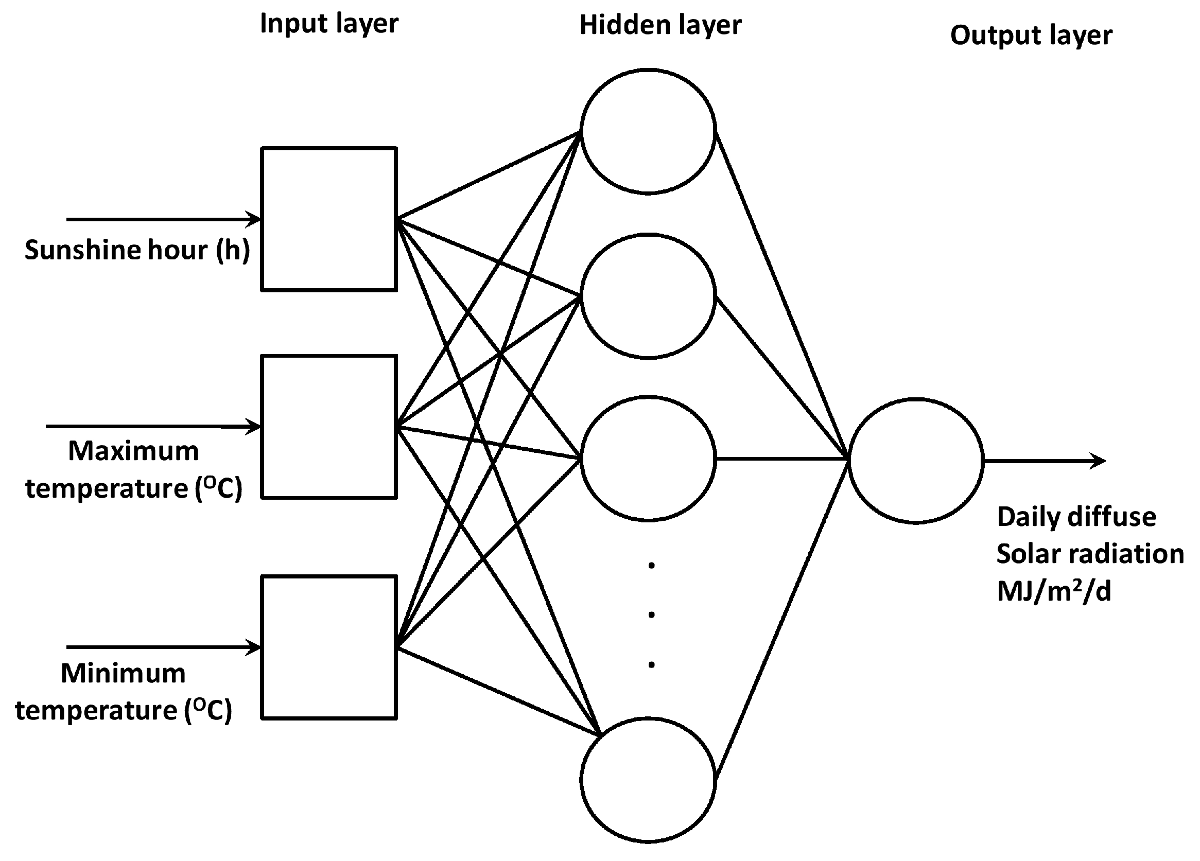
3.1. Artificial Neural Networks

Artificial neural networks are biologically inspired to mimic the structural sophistication and performance of the brain (biological neural system) used in computational machine learning purposes. Artificial neural networks comprise elements that are organized in a way comparable to that of the brain‘s anatomy and perform functions similar to that of a biological neuron. As such, models of artificial neural networks learn patterns intrinsic in observations in ways similar to that of the brain [50,51].
The perceptron is the basic artificial neural model that can learn [50,52,53]. A perceptron is composed of input units (congruous with the input signals which biological neuron receive); connection weights that can be trained and adjusted (congruous with the synapses in the biological neural system); processing element (consisting of summation function & activation function and congruous with soma in the biological neuron); bias (which is an additional input into the processing element); and an output unit (corresponding to output signal or response from the biological neuron). The perceptron is termed a single-layer neural network because it has only a layer of output unit [50]. The basic mathematical description of the perceptron is given in Equations (1) and (2).
y o = f i = 1 N w i v i + b o
= f ( w T v + b o ) 0
where v i , w i , y 0 , b o and w T denotes input signals, trainable synaptic weights, output signal, bias, synaptic weights transpose, respectively.
To generate an output from the perceptron, the product of each input and its synaptic weight is carried out. In basic ANN models, these products are summed and compared to a threshold before they are fed through the activation function that generates the output [53]. The activation function introduces non-linearity to the output of the artificial neuron. Without the activation function, the output signal will simply be linear and this may not always satisfy real-world interfaces [50,51,52,53]. The various activation functions used for ANN applications include: threshold logic unit, log sigmoid, tan sigmoid and the saturated linear activation function [50,51,52]. The overall aim of ANN training is reduction of overall error E r between the actual and predicted observations as expressed in Equation (3).
E r = 1 n E n
E n = 0 . 5 × ( D m F m ) 2
where D m and F m are the actual and predicted values for the m t h output processor, respectively, and  n is the total number of training patterns.
Training of ANNs can broadly be classified as supervised and unsupervised [53]. In supervised training, input-output pairs are supplied so that parameters of the network are adjusted in such a way that a specific input gives a target output. For unsupervised learning, the network is supplied only with the input data and self-organizes the data to decipher the collective pattern in it. Variants of these broad categories of learning exist [53,54]. In training artificial neural networks, learning algorithms such as Levenberg-Marquardt algorithm, backpropagation, Newton method, conjugate gradient, Quasi-Newton methods etc. are frequently used [53,55]. An artificial neural network is said to be well trained if it serves the purpose of reasonable generalization. For the purpose of effective generalization and enhanced approximation capability of ANN models, it is important that data are not over fitted during training. Data overfit can be avoided through complexity regularization by applying standard selection criteria such as the Akaike information criterion (AIC), Bayesian information criterion (BIC) and predictive stochastic complexity (PSC) [53,56]. Details of ANN implementation is available in the literature [34,57]. The structure of the proposed ANN model is shown in Figure 1. This ANN model is trained using DE.

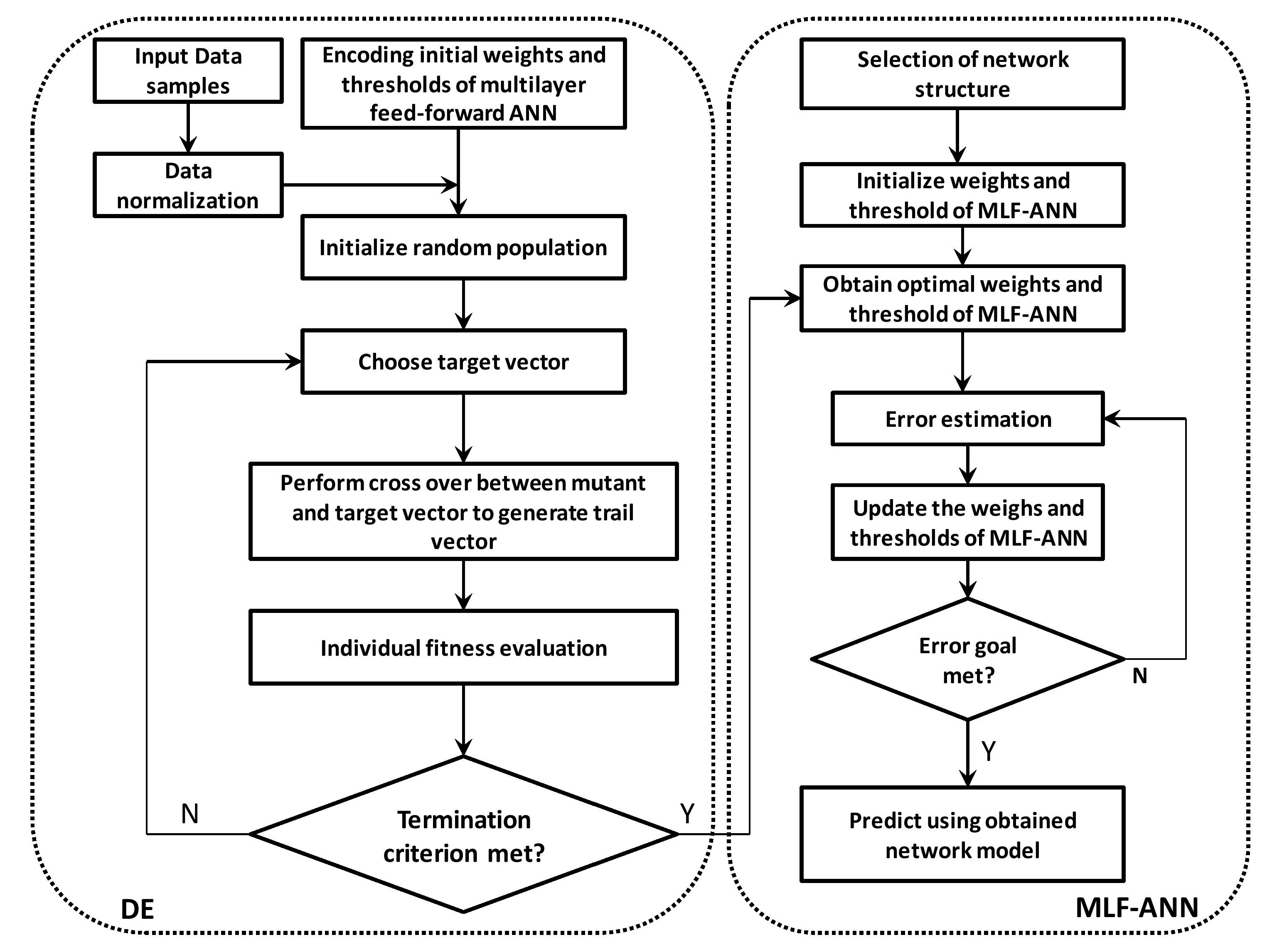
3.2. Differential Evolution

Differential evolution (DE) is a heuristic population-based parallel direct search algorithm optimization of continuous functions [36,58]. DE thrives on population of vectors which can independently be manipulated to perform the search. When the trial vector returns a lower objective function as compared to a predetermined population member, the trial vector that is recently generated will replace the vector and be compared in the next generation [59]. As this process continues, the convergence of the population is observed and the perturbations become less [60]. Based on this procedure, DE implements global search during the initial process and local search during the later phase of the process [59,60]. This feature makes DE capable of identifying the optimal weights needed for the minimization of error in ANN. [36]. The steps involved in DE is presented in Algorithm 1.
Algorithm 1: Classical Differential Evolution Algorithm
Energies 13 02488 i001

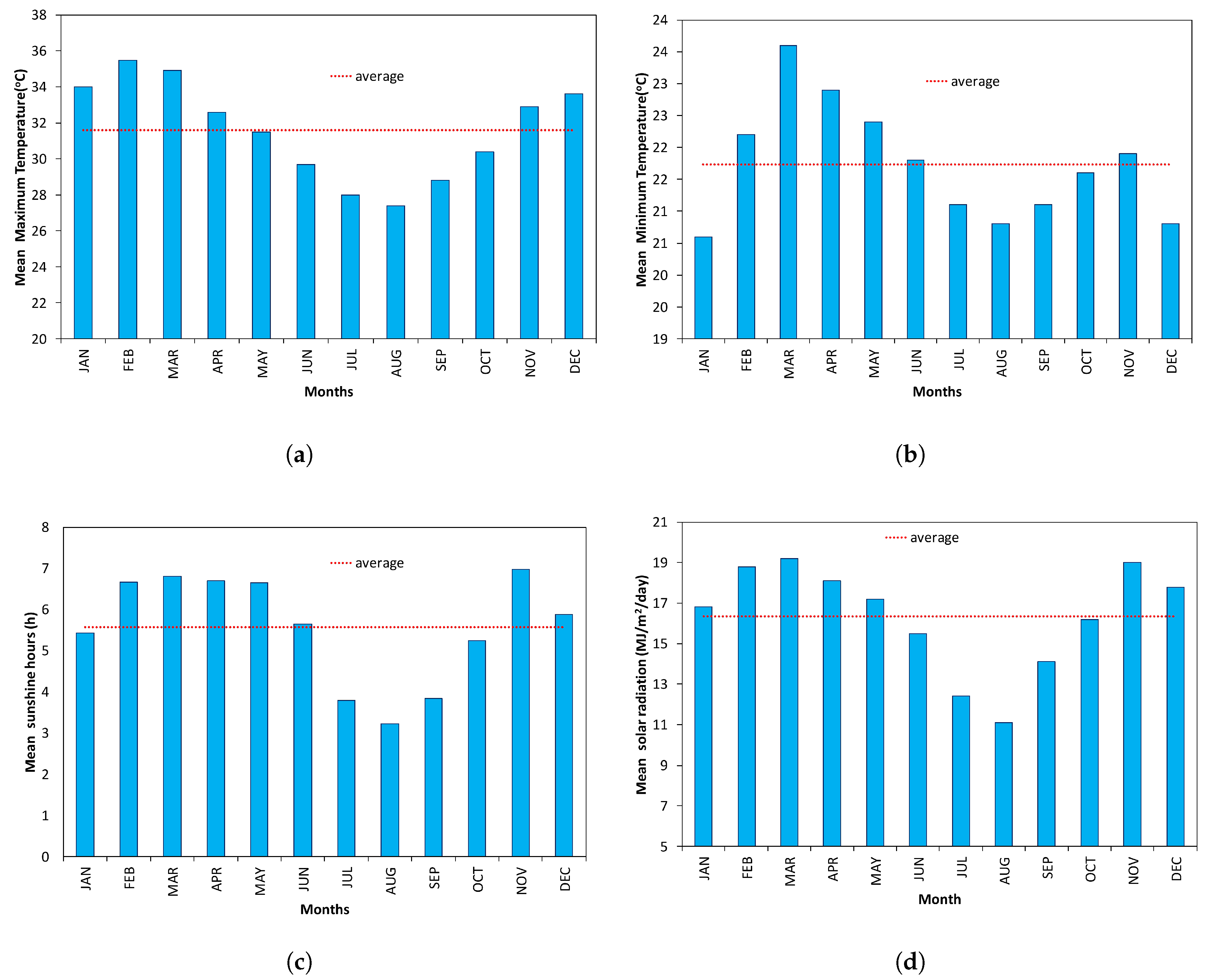
3.3. Site Description and Data Collection

The data used in the study were obtained from the national weather station (located in Iseyin) managed by the Nigerian meteorological agency. Iseyin (7 58 N 3 36 E) is a Nigerian city located in south-western part of the country and known for its commercial farming and mining activities. It has a population of more than 300 thousand people. The city is characterized by a tropical climate with a mean annual rainfall and ambient temperature of 1171 mm and 26.1 C respectively. Monthly average daily meteorological variables of global solar radiation ( H g ), maximum and minimum temperature ( T m a x , T m a x ) and sunshine hour ( S h ) for a 21 year period is obtained from the weather station (Figure 2).

3.4. Relation between Extraterrestrial and the Other Factors

The monthly average daily extraterrestrial radiation on a horizontal surface at the weather station can be obtained using Equations (5)–(9) [7,61].
H o = 24 π × I s c × w s s i n ϕ s i n δ + c o s ϕ c o s δ s i n w s × d r
N ¯ = 2 15 × w s
δ = 23 . 4 s i n 360 × ( 284 + d ) 365
w s = c o s 1 ( t a n ϕ t a n δ )
d r = 1 + 0 . 033 c o s 360 × d 365
where I s c , w s , d r , H o , δ , N ¯ , d and ϕ are the solar constant, hour angle, inverse relative distance of the sun to earth, monthly mean daily extraterrestrial solar radiation, solar declination, monthly daylight hour, day number, and latitude of the site under consideration respectively.

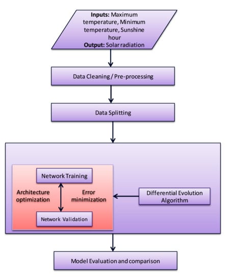
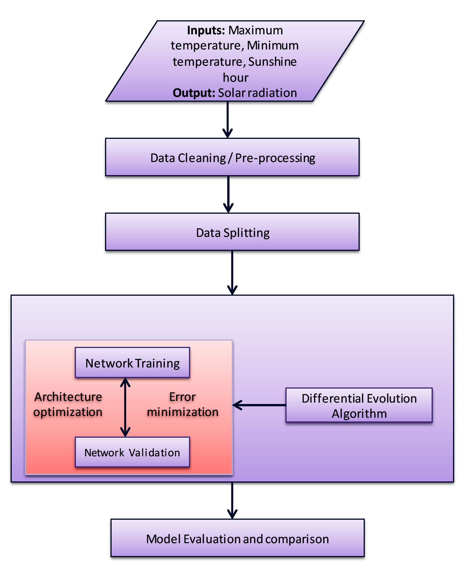
3.5. Model Development

The procedural steps used in modelling solar radiation at a monthly timescale is presented in this section. These steps summarized in a methodological framework and illustrated in Figure 3 entailed the use of a classic DE algorithm in training a MLF-ANN.

3.5.1. Network Typology and Setup

The architectural layout of the MLF-ANN developed in this study comprised three layers: one input and output layer as well as a single hidden layer which comprises neurons. A logistic sigmoidal-type activation function [0, 1] was utilized in the hidden layer of the MLF-ANN to rescale the inputs in an interval [0.1, 0.9] while a linear activation function was adopted in the output layer. The monthly averages of daily sunshine duration, minimum and maximum temperatures were used in developing the input layer of the ANN architecture while the corresponding averages of solar radiation were used to construct the output layer (i.e., the target output). Consequently, the MLF-ANN was characterized by three input layer neurons and one output layer neuron. Equation (10) describes the functional relationship between solar radiation and the input variables considered in this study.
H g = f ( S h , T m i n , T m a x )

3.5.2. Data Splitting

In data-driven modelling, the standard is to split a given set of historical observations into training and testing sets [34]. The total number of observations for the study area from year 1987 to 2007 and utilized for training and validation (testing) is 250. The data set was divided into two grouped that exhibit analogous statistical features with 200 (80%) observations used for model training and the outstanding 50 (30%) observations for testing. Table 2 presents the statistical properties of the training and testing data sets.

3.5.3. Model Implementation and Optimization

Considering the fact that network complexity is dependent on the number of neurons in hidden layer, a decision was taken to not predefine the number of hidden layer neurons for the MLF-ANN. Alternatively, using the DE algorithm, the hidden layer was subjected to a sensitivity analysis which involved varying the number of processing neurons incrementally between 1 to 10, utilizing a single step function and observing the error profile at each stage. DE was therefore used to optimize the network parameters (i.e., the synaptic weights and biases) and network architecture of model. In training the MLF-ANN, the DE algorithm run was initially run for 100 generations. The parameters used in governing the algorithm run include population size (NP), crossover probability (CR) and mutation probability (F). NP was set at “D × 10” ( the number of weights and bias is D) while a search for the optimal values of CR and F was performed within the range [0.1, 0.9] to determine the best combination of parameter setting. The best parameter setting obtained from the initial run (CR = 0.9 and F = 0.4) was thereafter used in performing a finer search with the DE algorithm initialized for 10,000 generations. The DE algorithm was therefore aimed at optimizing model accuracy and model complexity simultaneously to foster a mutual accommodation between both objectives. To mitigate the risk of over-fitting which ANN models typically suffer from, an early-stopping function which detects the point where the least error on the test data set starts to increase and immediately stops training was introduced [36].

3.5.4. Model Performance Evaluation

The prediction performance and accuracy of the proposed model is evaluated using three statistical metrics, which include [36,62,63]:
  • Root-mean-square error:
    R M S E = i = 1 X ( D i F ¯ i ) 2 x
  • Coefficient of determination:
    R 2 = i = 1 X ( D i D ¯ i ) ( F i F ¯ i ) i = 1 X ( D i D ¯ i ) 2 . i = 1 X ( F i F ¯ i ) 2 2
  • Nash-Sutcliffe efficiency index:
    N S E = 1 i = 1 X ( D i F i ) 2 i = 1 X ( D ¯ i D i ) 2
    where the observed and predicted values are given as D i and F i respectively and their mean values are given as D ¯ i and F ¯ i respectively and X is the data size.

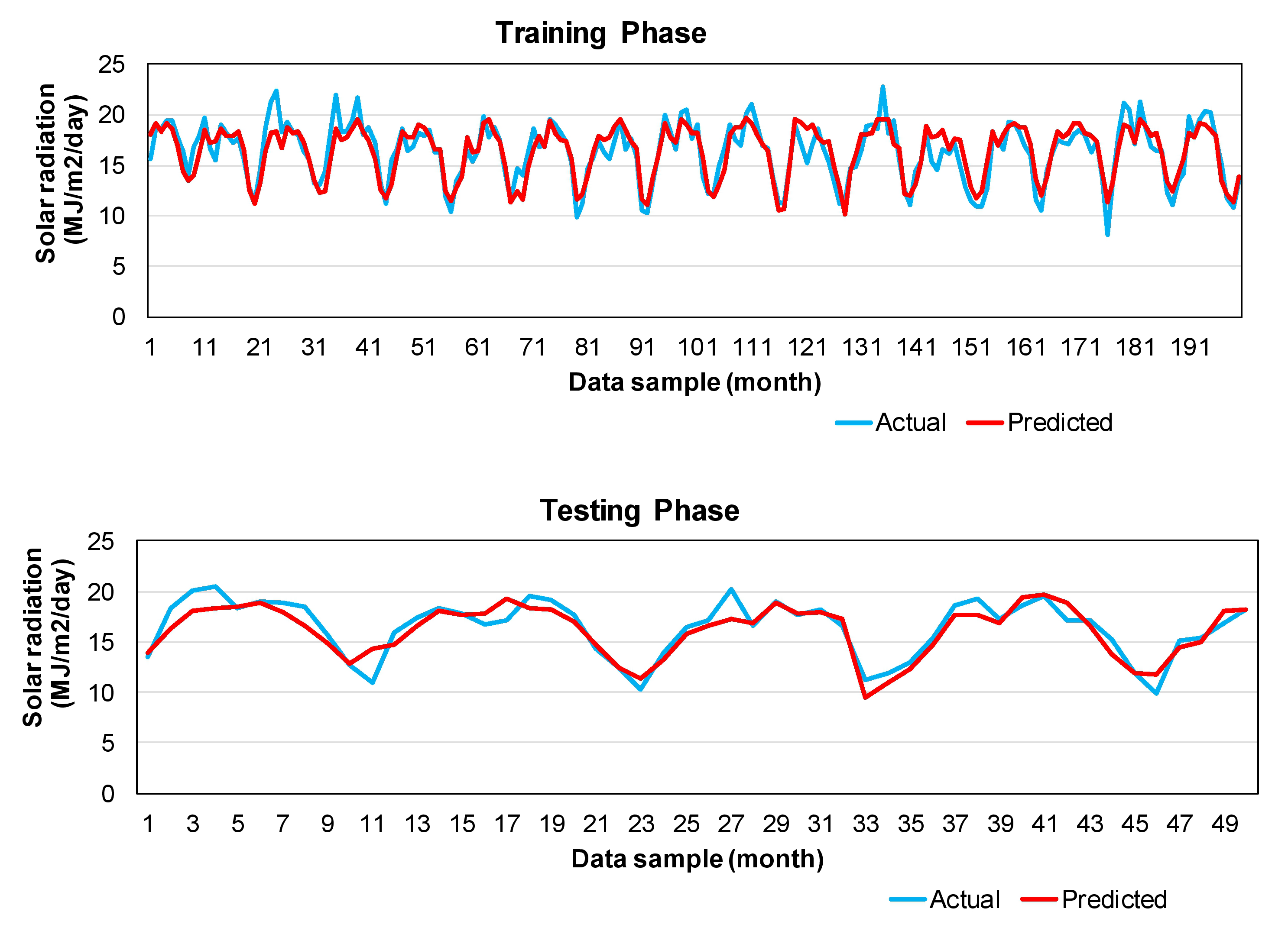
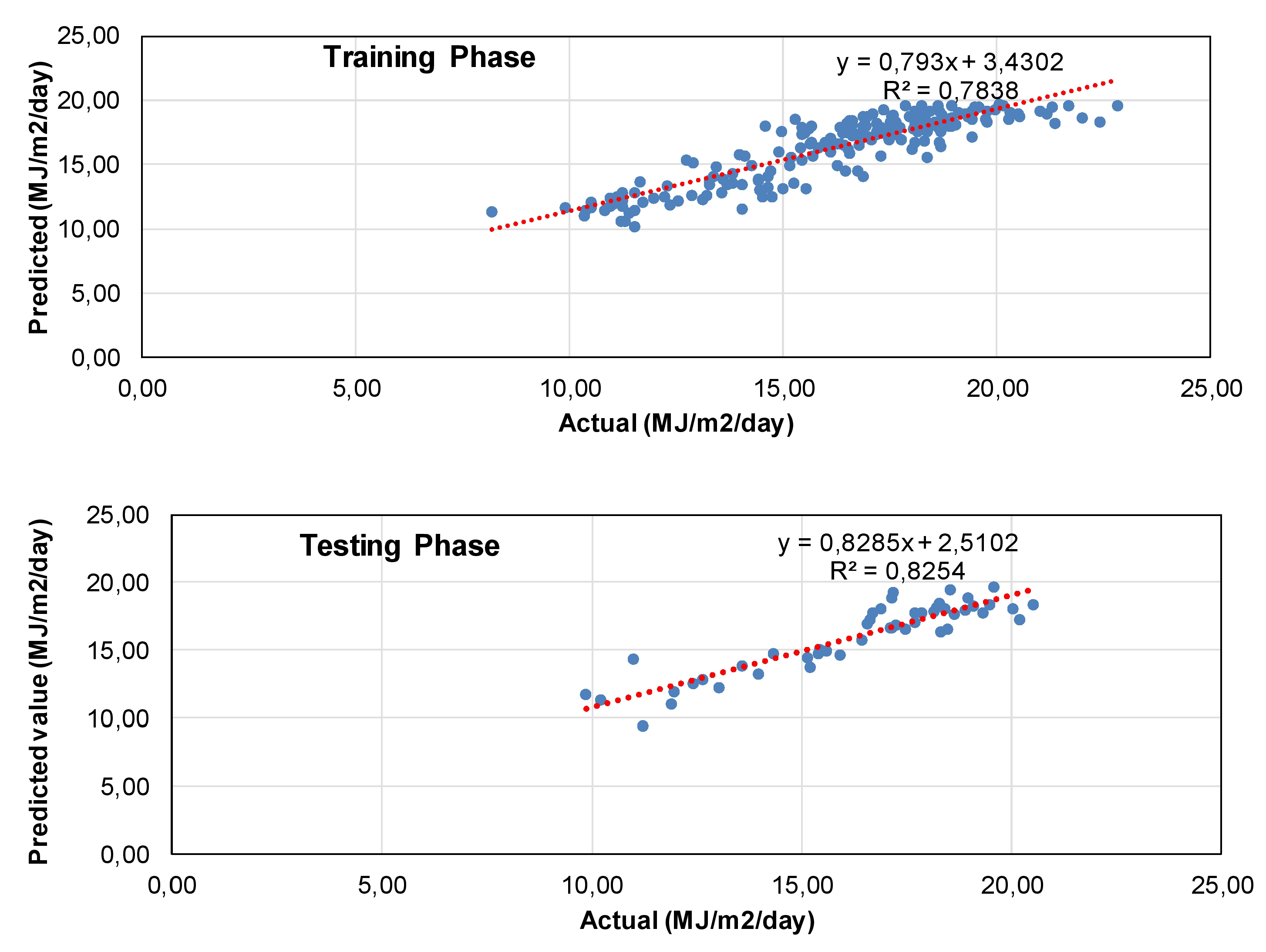
4. Results and Discussion

The efficacy of the proposed ANN-DE model was appraised based on two metrics- accuracy and complexity. The results with respect to model accuracy is presented in Table 3. Table 3 show that a minimal model error occurred during training, producing a RMSE of 1.3292. R 2 and NSE values were estimated to be 0.7838 and 0.7835 respectively, signifying high model accuracy during training. During the testing phase, an improvement in the model performance metrics (RMSE = 1.196; R 2 = 0.8254; NSE = 0.8134) can be observed. This translates to a 11%, 5.3% and 3.8% improvement in model performance during testing, respectively.
These results imply that the model did not only produce an accurate representation of solar radiation of the City but has showcased good model generalization and convergence across the training and testing phases of the simulation. This is an indication that the ANN model did not encounter over-fitting problems which typically plagues conventional ANN models. The remarkable performance of the ANN model can be attributed to the robustness of the DE algorithm via its genetic operators, ensuring a productive exploration in estimating the network parameters (weight and biases) of the model. The adoption of the early stopping technique also served as a good complement as it ensured that training is halted as soon as an increase in error is observed to prevent over-fitting. With regards to complexity, the DE algorithm ensured that model accuracy is obtained at minimal model complexity as the optimal number of hidden layer neurons returned after exploration [1, 10] is three. Hence, the optimal network architecture of the ANN is 3-3-1. This signifies that the model accuracy was obtained using minimal computational resources.
Figure 4 and Figure 5 present a visual representation of the model performance in predicting solar radiation for the City of Iseyin over the study period. Figure 4 shows plots of actual and predicted values of solar radiation during training and testing. The chart visibly indicates that the proposed model created a good replica of the solar radiation pattern for Iseyin. Majority of the troughs and crests were reproduced by the model. Only a limited number of under- and over-estimations can be observed. The corresponding scatter plots also shows a positive correlation and high accuracy between the predicted and actual values- R 2 is 0.7838 at the training phase, while R 2 is 0.8254 for the testing phase (Figure 5).
To further evaluate the performance of the ANN model, the results obtained from this study were compared with results reported in Olatomiwa et al. (2015) [7]. In their study, the authors employed seven soft computing techniques to estimate monthly solar radiation for the same location and period used in this study. The models reported in their study were developed using the following techniques: SVR with polynomial kernel function (SVR-polynomial), SVR with radial basis function kernel (SVR-radial), ANFIS coupled with ant colony optimization (ANFIS-ACO), ANFIS coupled with differential evolution (ANFIS-DE), ANFIS coupled with genetic algorithm (ANFIS-GA), ANFIS coupled with particle swarm optimization (ANFIS-PSO), and ANFIS. Table 4 presents results from the comparative analysis. It can be observed from the results that, although all the models performed well during training, they were all unable to produce the same or a better performance during testing. All the seven models produced higher RMSE values during testing than those produced during training. Similarly, the estimated R 2 values during testing phase were lower than those estimated during training. This denotes that all the models were plagued to some degree by over-fitting, resulting in inadequate generalization. In fact, the SVR-radial, ANFIS-PSO and ANFIS models suffered severely from over-fitting. On the other hand, the ANN model developed in this study recorded an improved performance between the training and testing phases. It can be concluded from the comparative analysis that the ANN model developed in this study clearly outperformed the seven models reported in Olatomiwa et al. (2015) [7].
To further assess the performance of the ANN model developed in this study, its prediction accuracy was compared against eight existing studies in the literature undertaken in different regions across the world (Table 5). Techniques employed in the compared models comprise both empirical and soft computing techniques. The performance of the models was evaluated based on R 2 estimates. The comparison results show that the ANN model developed in this study (trained using DE) provided superior results than the other models compared in this study. The combined use of DE and early stopping can be considered as instrumental in enhancing the efficiency of the ANN model, providing high accuracy at minimal complexity. This paper has been able to elucidate the capability of differential evolution in training artificial neural network for solar radiation prediction.

5. Conclusions

The decarbonization of the energy sector has led to extensive research and technological development with respect to the use of solar energy for electricity generation. As such, solar technologies like solar photovoltaics (PV), concentrated solar power (CSP), solar hybrid systems (solar-hydrogen, solar-diesel generator, solar-wind etc.), concentrator photovoltaics (CPV) etc are presently being used to generate electricity either in small scale or commercial quantity. In all cases and technologies, solar radiation data is a very essential input parameter during design and modelling. This is usually not available or incomplete. One way of obtaining solar radiation data is from historical data, through the use of predictive tools. In order to elucidate the efficacy of the proposed ANN-DE model in predicting solar radiation in the presence of limited data set, 3 input parameters ( T m a x , T m a x and S h ) and 3 performance ( R 2 , RMSE and NSE) metrics were used. The performance metrics obtained from the proposed ANN-DE model show superior performance with respect to the error values returned when compared to existing models that have been used in the area under consideration. It is worth noting that the values of these performance metrics may change with change in location and data. This is one of the drawbacks of all data driven techniques [21]. The proposed model has the capability of predicting solar radiation that can be used as input for various solar powered projects at the location where the data are recorded. The methodology adopted in this model can be tested at other locations to ascertain its universality. Future studies could also look into the use of DE and other meta-heuristic approaches in training ANN for solar radiation prediction at finer timescales.

Author Contributions

O.M.B. formulated the problem and drafted the manuscript. J.L.M. and Y.H. assisted with quality improvement. All authors have read and agreed to the published version of the manuscript.

Funding

This work is based on the research supported in part by the National Research Foundation of South Africa (Grant Number: 121078). Opinions expressed and conclusions arrived at, are those of the authors and are not necessarily to be attributed to the NRF.

Acknowledgments

The first author appreciate the useful discussions and insightful inputs of Oluwaseun Oyebode. The first author also appreciate Olatomiwa Lanre for helping out with the raw data.

Conflicts of Interest

The authors declare no conflict of interest.

Abbreviations

Symbol/AcronymDescription
P a i r Air Pressure
MSEMean square error
A L Altitude
T a v e Mean/average Temperature
C a v e Average daily cloudiness
T m i n Minimum Temperature
P a v e Average Pressure
T m a x Maximum Temperature
C i Clearness index
EFModel Efficiency
n C i , g C i Clearness index and global clearness index respectively
MMonth
R 2 Coefficient of determination
NSNash–Sutcliffe coefficient
RCorrelation coefficient
nRMSENormalized root mean square error
DDay
nMBENormalized mean bias error
E r Extraterrestrial radiation on a horizontal surface
PPressure
GPIGlobal performance index
R p r e p Rainfall/precipitation
G s r Global solar radiation
RERelative error
L a , L o Latitude, Longitude
H r Relative humidity
S h m a x Maximum sunshine hour
RRMSERelative root mean square error
MAEMean absolute error
RMSERoot mean square error
MPBEMean Absolute Percentage Error
S h Sunshine hour
MABEMean absolute bias error
TTemperature
MAPEMean absolute percentage error
T O A I Top of atmosphere insolation
MBEMean bias error
P w v Water vapour pressure
MPEMean percentage error
V w Wind Speed

References

  1. Wassie, Y.T.; Adaramola, M.S. Potential environmental impacts of small-scale renewable energy technologies in East Africa: A systematic review of the evidence. Renew. Sustain. Energy Rev. 2019, 111, 377–391. [Google Scholar] [CrossRef]
  2. Babatunde, O.; Akinyele, D.; Akinbulire, T.; Oluseyi, P. Evaluation of a grid-independent solar photovoltaic system for primary health centres (PHCs) in developing countries. Renew. Energy Focus 2018, 24, 16–27. [Google Scholar] [CrossRef]
  3. Olatomiwa, L. Optimal configuration assessments of hybrid renewable power supply for rural healthcare facilities. Energy Rep. 2016, 2, 141–146. [Google Scholar] [CrossRef] [Green Version]
  4. Ipsakis, D.; Voutetakis, S.; Seferlis, P.; Stergiopoulos, F.; Elmasides, C. Power management strategies for a stand-alone power system using renewable energy sources and hydrogen storage. Int. J. Hydrog. Energy 2009, 34, 7081–7095. [Google Scholar] [CrossRef]
  5. Samy, M.; Barakat, S.; Ramadan, H. Techno-economic analysis for rustic electrification in Egypt using multi-source renewable energy based on PV/wind/FC. Int. J. Hydrog. Energy 2019, 45, 11471–11483. [Google Scholar] [CrossRef]
  6. Mohammadi, K.; Shamshirband, S.; Kamsin, A.; Lai, P.; Mansor, Z. Identifying the most significant input parameters for predicting global solar radiation using an ANFIS selection procedure. Renew. Sustain. Energy Rev. 2016, 63, 423–434. [Google Scholar] [CrossRef]
  7. Olatomiwa, L.; Mekhilef, S.; Shamshirband, S.; Petković, D. Adaptive neuro-fuzzy approach for solar radiation prediction in Nigeria. Renew. Sustain. Energy Rev. 2015, 51, 1784–1791. [Google Scholar] [CrossRef]
  8. Kuo, P.H.; Chen, H.C.; Huang, C.J. Solar Radiation Estimation Algorithm and Field Verification in Taiwan. Energies 2018, 11, 1374. [Google Scholar] [CrossRef] [Green Version]
  9. Mauleón, I. Assessing PV and wind roadmaps: Learning rates, risk, and social discounting. Renew. Sustain. Energy Rev. 2019, 100, 71–89. [Google Scholar] [CrossRef]
  10. IRENA. Renewable Power Generation Costs in 2017; International Renewable Energy Agency (IRENA): Abu Dhabi, UAE, 2018. [Google Scholar]
  11. Ayodele, T.; Munda, J. Potential and economic viability of green hydrogen production by water electrolysis using wind energy resources in South Africa. Int. J. Hydrog. Energy 2019, 44, 17669–17687. [Google Scholar] [CrossRef]
  12. Allahvirdizadeh, Y.; Mohamadian, M.; HaghiFam, M.R. Study of energy control strategies for a standalone PV/FC/UC microgrid in a remote. Int. J. Renew. Energy Res. (IJRER) 2017, 7, 1495–1508. [Google Scholar]
  13. Saadi, A.; Becherif, M.; Ramadan, H. Hydrogen production horizon using solar energy in Biskra, Algeria. Int. J. Hydrog. Energy 2016, 41, 21899–21912. [Google Scholar] [CrossRef]
  14. Rezaei, M.; Mostafaeipour, A.; Qolipour, M.; Momeni, M. Energy supply for water electrolysis systems using wind and solar energy to produce hydrogen: A case study of Iran. Front. Energy 2019, 13, 539–550. [Google Scholar] [CrossRef]
  15. Mohamed, B.; Ali, B.; Ahmed, B.; Ahmed, B.; Salah, L.; Rachid, D. Study of hydrogen production by solar energy as tool of storing and utilization renewable energy for the desert areas. Int. J. Hydrog. Energy 2016, 41, 20788–20806. [Google Scholar] [CrossRef]
  16. Menad, C.A.; Gomri, R.; Bouchahdane, M. Data on safe hydrogen production from the solar photovoltaic solar panel through alkaline electrolyser under Algerian climate. Data Brief 2018, 21, 1051–1060. [Google Scholar] [CrossRef]
  17. Sigal, A.; Leiva, E.P.M.; Rodríguez, C. Assessment of the potential for hydrogen production from renewable resources in Argentina. Int. J. Hydrog. Energy 2014, 39, 8204–8214. [Google Scholar] [CrossRef]
  18. Contreras, A.; Guirado, R.; Veziroglu, T. Design and simulation of the power control system of a plant for the generation of hydrogen via electrolysis, using photovoltaic solar energy. Int. J. Hydrog. Energy 2007, 32, 4635–4640. [Google Scholar] [CrossRef]
  19. Yaniktepe, B.; Genc, Y.A. Establishing new model for predicting the global solar radiation on horizontal surface. Int. J. Hydrog. Energy 2015, 40, 15278–15283. [Google Scholar] [CrossRef]
  20. Kaur, A.; Nonnenmacher, L.; Pedro, H.T.; Coimbra, C.F. Benefits of solar forecasting for energy imbalance markets. Renew. Energy 2016, 86, 819–830. [Google Scholar] [CrossRef]
  21. Halawa, E.; GhaffarianHoseini, A.; Li, D.H.W. Empirical correlations as a means for estimating monthly average daily global radiation: A critical overview. Renew. Energy 2014, 72, 149–153. [Google Scholar] [CrossRef]
  22. Bocca, A.; Bergamasco, L.; Fasano, M.; Bottaccioli, L.; Chiavazzo, E.; Macii, A.; Asinari, P. Multiple-regression method for fast estimation of solar irradiation and photovoltaic energy potentials over Europe and Africa. Energies 2018, 11, 3477. [Google Scholar] [CrossRef] [Green Version]
  23. Feng, Y.; Cui, N.; Zhang, Q.; Zhao, L.; Gong, D. Comparison of artificial intelligence and empirical models for estimation of daily diffuse solar radiation in North China Plain. Int. J. Hydrog. Energy 2017, 42, 14418–14428. [Google Scholar] [CrossRef]
  24. Xue, X. Prediction of daily diffuse solar radiation using artificial neural networks. Int. J. Hydrog. Energy 2017, 42, 28214–28221. [Google Scholar] [CrossRef]
  25. Alsina, E.F.; Bortolini, M.; Gamberi, M.; Regattieri, A. Artificial neural network optimisation for monthly average daily global solar radiation prediction. Energy Convers. Manag. 2016, 120, 320–329. [Google Scholar] [CrossRef]
  26. Hussain, S.; AlAlili, A. A hybrid solar radiation modeling approach using wavelet multiresolution analysis and artificial neural networks. Appl. Energy 2017, 208, 540–550. [Google Scholar] [CrossRef]
  27. Gairaa, K.; Khellaf, A.; Messlem, Y.; Chellali, F. Estimation of the daily global solar radiation based on Box–Jenkins and ANN models: A combined approach. Renew. Sustain. Energy Rev. 2016, 57, 238–249. [Google Scholar] [CrossRef]
  28. Mousavi Maleki, S.A.; Hizam, H.; Gomes, C. Estimation of hourly, daily and monthly global solar radiation on inclined surfaces: Models re-visited. Energies 2017, 10, 134. [Google Scholar] [CrossRef] [Green Version]
  29. Fan, J.; Wang, X.; Wu, L.; Zhang, F.; Bai, H.; Lu, X.; Xiang, Y. New combined models for estimating daily global solar radiation based on sunshine duration in humid regions: A case study in South China. Energy Convers. Manag. 2018, 156, 618–625. [Google Scholar] [CrossRef]
  30. Yacef, R.; Mellit, A.; Belaid, S.; Şen, Z. New combined models for estimating daily global solar radiation from measured air temperature in semi-arid climates: Application in Ghardaïa, Algeria. Energy Convers. Manag. 2014, 79, 606–615. [Google Scholar] [CrossRef]
  31. Fan, J.; Wang, X.; Wu, L.; Zhou, H.; Zhang, F.; Yu, X.; Lu, X.; Xiang, Y. Comparison of Support Vector Machine and Extreme Gradient Boosting for predicting daily global solar radiation using temperature and precipitation in humid subtropical climates: A case study in China. Energy Convers. Manag. 2018, 164, 102–111. [Google Scholar] [CrossRef]
  32. Hussain, S.; Al-Alili, A. A new approach for model validation in solar radiation using wavelet, phase and frequency coherence analysis. Appl. Energy 2016, 164, 639–649. [Google Scholar] [CrossRef]
  33. Hassan, M.A.; Khalil, A.; Kaseb, S.; Kassem, M. Exploring the potential of tree-based ensemble methods in solar radiation modeling. Appl. Energy 2017, 203, 897–916. [Google Scholar] [CrossRef]
  34. Oyebode, O.; Stretch, D. Neural network modeling of hydrological systems: A review of implementation techniques. Nat. Resour. Model. 2019, 32, e12189. [Google Scholar] [CrossRef] [Green Version]
  35. Oyebode, O.; Ighravwe, D.E. Urban Water Demand Forecasting: A Comparative Evaluation of Conventional and Soft Computing Techniques. Resources 2019, 8, 156. [Google Scholar] [CrossRef] [Green Version]
  36. Oyebode, O. Evolutionary modelling of municipal water demand with multiple feature selection techniques. J. Water Supply Res. Technol. AQUA 2019, 68, 264–281. [Google Scholar] [CrossRef] [Green Version]
  37. Yorukoglu, M.; Celik, A.N. A critical review on the estimation of daily global solar radiation from sunshine duration. Energy Convers. Manag. 2006, 47, 2441–2450. [Google Scholar] [CrossRef]
  38. Zhang, J.; Zhao, L.; Deng, S.; Xu, W.; Zhang, Y. A critical review of the models used to estimate solar radiation. Renew. Sustain. Energy Rev. 2017, 70, 314–329. [Google Scholar] [CrossRef]
  39. Halabi, L.M.; Mekhilef, S.; Hossain, M. Performance evaluation of hybrid adaptive neuro-fuzzy inference system models for predicting monthly global solar radiation. Appl. Energy 2018, 213, 247–261. [Google Scholar] [CrossRef]
  40. Baser, F.; Demirhan, H. A fuzzy regression with support vector machine approach to the estimation of horizontal global solar radiation. Energy 2017, 123, 229–240. [Google Scholar] [CrossRef]
  41. Fan, J.; Chen, B.; Wu, L.; Zhang, F.; Lu, X.; Xiang, Y. Evaluation and development of temperature-based empirical models for estimating daily global solar radiation in humid regions. Energy 2018, 144, 903–914. [Google Scholar] [CrossRef]
  42. Khosravi, A.; Koury, R.; Machado, L.; Pabon, J. Prediction of hourly solar radiation in Abu Musa Island using machine learning algorithms. J. Clean. Prod. 2018, 176, 63–75. [Google Scholar] [CrossRef]
  43. Khosravi, A.; Nunes, R.; Assad, M.; Machado, L. Comparison of artificial intelligence methods in estimation of daily global solar radiation. J. Clean. Prod. 2018, 194, 342–358. [Google Scholar] [CrossRef]
  44. Zou, L.; Wang, L.; Xia, L.; Lin, A.; Hu, B.; Zhu, H. Prediction and comparison of solar radiation using improved empirical models and Adaptive Neuro-Fuzzy Inference Systems. Renew. Energy 2017, 106, 343–353. [Google Scholar] [CrossRef]
  45. Akarslan, E.; Hocaoglu, F.O. A novel adaptive approach for hourly solar radiation forecasting. Renew. Energy 2016, 87, 628–633. [Google Scholar] [CrossRef]
  46. Rohani, A.; Taki, M.; Abdollahpour, M. A novel soft computing model (Gaussian process regression with K-fold cross validation) for daily and monthly solar radiation forecasting (Part: I). Renew. Energy 2018, 115, 411–422. [Google Scholar] [CrossRef]
  47. Mohammadi, K.; Shamshirband, S.; Petković, D.; Khorasanizadeh, H. Determining the most important variables for diffuse solar radiation prediction using adaptive neuro-fuzzy methodology; case study: City of Kerman, Iran. Renew. Sustain. Energy Rev. 2016, 53, 1570–1579. [Google Scholar] [CrossRef]
  48. Wang, L.; Kisi, O.; Zounemat-Kermani, M.; Salazar, G.A.; Zhu, Z.; Gong, W. Solar radiation prediction using different techniques: Model evaluation and comparison. Renew. Sustain. Energy Rev. 2016, 61, 384–397. [Google Scholar] [CrossRef]
  49. Zou, L.; Wang, L.; Lin, A.; Zhu, H.; Peng, Y.; Zhao, Z. Estimation of global solar radiation using an artificial neural network based on an interpolation technique in southeast China. J. Atmos. Sol.-Terr. Phys. 2016, 146, 110–122. [Google Scholar] [CrossRef]
  50. Suk, H.I. An introduction to neural networks and deep learning. In Deep Learning for Medical Image Analysis; Elsevier: Amsterdam, The Netherlands, 2017; pp. 3–24. [Google Scholar]
  51. Teodorovic, D.; Janic, M. Transportation Engineering: Theory, Practice and Modeling; Butterworth-Heinemann: Oxford, UK, 2016. [Google Scholar]
  52. Majumdar, A. Soft Computing in Textile Engineering; Elsevier: Amsterdam, The Netherlands, 2010. [Google Scholar]
  53. Babatunde, D.E.; Anozie, A.; Omoleye, J. Artificial Neural Network and its Applications in the Energy Sector—An Overview. Int. J. Energy Econ. Policy 2020, 10, 250–264. [Google Scholar] [CrossRef]
  54. Awodele, O.; Jegede, O. Neural networks and its application in engineering. In Proceedings of the Informing Science & IT Education Conference (InSITE), Macon, GA, USA, 12–15 June 2009; pp. 83–95. [Google Scholar]
  55. Livieris, I.; Pintelas, P. A Survey on Algorithms for Training Artificial Neural Networks; University of Patras: Patras, Greece, 2008; Volume 4. [Google Scholar]
  56. Nisbet, R.; Elder, J.; Miner, G. Handbook of Statistical Analysis and Data Mining Applications; Academic Press: Cambridge, MA, USA, 2009. [Google Scholar]
  57. Shahin, M.A.; Jaksa, M.B.; Maier, H.R. State of the art of artificial neural networks in geotechnical engineering. Electron. J. Geotech. Eng. 2008, 8, 1–26. [Google Scholar]
  58. Storn, R.; Price, K. Differential evolution–a simple and efficient heuristic for global optimization over continuous spaces. J. Glob. Optim. 1997, 11, 341–359. [Google Scholar] [CrossRef]
  59. Li, X.; Yin, M. Application of differential evolution algorithm on self-potential data. PLoS ONE 2012, 7, e51199. [Google Scholar] [CrossRef] [PubMed]
  60. Yang, S.; Natarajan, U.; Sekar, M.; Palani, S. Prediction of surface roughness in turning operations by computer vision using neural network trained by differential evolution algorithm. Int. J. Adv. Manuf. Technol. 2010, 51, 965–971. [Google Scholar] [CrossRef]
  61. Olatomiwa, L.; Mekhilef, S.; Shamshirband, S.; Petkovic, D. Potential of support vector regression for solar radiation prediction in Nigeria. Nat. Hazards 2015, 77, 1055–1068. [Google Scholar] [CrossRef]
  62. Khorasanizadeh, H.; Mohammadi, K.; Goudarzi, N. Prediction of horizontal diffuse solar radiation using clearness index based empirical models; A case study. Int. J. Hydrog. Energy 2016, 41, 21888–21898. [Google Scholar] [CrossRef]
  63. Olatomiwa, L.; Mekhilef, S.; Shamshirband, S.; Mohammadi, K.; Petković, D.; Sudheer, C. A support vector machine–firefly algorithm-based model for global solar radiation prediction. Sol. Energy 2015, 115, 632–644. [Google Scholar] [CrossRef]
  64. Abdalla, Y.A. New correlations of global solar radiation with meteorological parameters for Bahrain. Int. J. Sol. Energy 1994, 16, 111–120. [Google Scholar] [CrossRef]
  65. Angstrom, A. Solar and terrestrial radiation. Report to the international commission for solar research on actinometric investigations of solar and atmospheric radiation. Q. J. R. Meteorol. Soc. 1924, 50, 121–126. [Google Scholar] [CrossRef]
  66. Bahel, V.; Bakhsh, H.; Srinivasan, R. A correlation for estimation of global solar radiation. Energy 1987, 12, 131–135. [Google Scholar] [CrossRef]
  67. Bakirci, K. Correlations for estimation of daily global solar radiation with hours of bright sunshine in Turkey. Energy 2009, 34, 485–501. [Google Scholar] [CrossRef]
  68. Ramedani, Z.; Omid, M.; Keyhani, A.; Shamshirband, S.; Khoshnevisan, B. Potential of radial basis function based support vector regression for global solar radiation prediction. Renew. Sustain. Energy Rev. 2014, 39, 1005–1011. [Google Scholar] [CrossRef]
  69. Yohanna, J.K.; Itodo, I.N.; Umogbai, V.I. A model for determining the global solar radiation for Makurdi, Nigeria. Renew. Energy 2011, 36, 1989–1992. [Google Scholar] [CrossRef]
Figure 1. Structure of multilayer feed-foward ANN model.
Energies 13 02488 g001
Figure 2. Meteorological features of the site. (a) Mean maximum temperature; (b) Mean minimum temperature; (c) Mean sunshine hour; (d) Mean solar radiation.
Energies 13 02488 g002
Figure 3. Methodological framework.
Energies 13 02488 g003
Figure 4. Plots of actual and predicted values of solar radiation during training and testing.
Energies 13 02488 g004
Figure 5. Scatter plots of training data and predicted values.
Energies 13 02488 g005
Table 1. Comparison of literature.
AuthorMethodInput ParametersPerformance MetricsLocation
[19]linear, second
third order polynomial
E r , S h MAPE, MABE,
RMSE
Turkey
[23]ELM, BPNN-GA,
BPNN-RF, GRNN
G s r , S h , max. S h , E r RRMSE, MAE,
RE, NS
China
[24]BPNN-PSO, BPNN-GA G s r , M, T a v e , R p r e p , H r ,
S h , V w
R, RMSE, MAEChina
[25]ANN-spatial interpolation A L , C a v e , d, S h , R p r e p , T O A I , d,
clear sky days, heating degrees day,
L o , L a , M, rainy days
MAPE, NRMSE,
MPBE
Italy
[26]ANFIS, GRNN, MLP, NARX H r , S h , T a v e , V w R 2 , RMSE,
MAPE, MBE
United Arab
Emirates
[27]ARMA, NANN C i RMSE, nRMSE, MBE,
nMBE, MPE, R 2
Algeria
[29]Temperature-based models (TBM) T a v e , G s r , R p r e p , S h R 2 , RMSE, NRMSE,
MBE, GPI
China
[30]empirical models, BNN H r , G s r , TRMSE, MBE, MAE, RAlgeria
[31]EGB, SVMT, R, E r RMSE, MBE, MAE,China
[32]ANN, MLP-ANN, ANFIS,
NARX-NN
V w , S h , H r , T a v e MAPE, R 2 , RMSEUnited Arab
Emirates
[33]GBB and RF G s r , n C i , d, g C i ,
sunshine fraction, diffuse fraction
MBE, RMSE, R 2 ,Middle East,
North Africa
[39]ANFIS-GA, ANFIS-PSO,
ANFIS-DE
C i , T m a x , T m i n , R p r e p , S h MAPE, RRMSE,
MABE, R 2 , RMSE, R
Malyasia
[40]fuzzy regression functions-SVMlatitude, longitude, T a v e , H r , G s r RMSE, MAETurkey
[41]TBM V w , G s r , T m i n ,
T m a x , R p r e p , H r
R 2 , RMSE, NRMSE,
MBE, GPI
China
[42]SVR, RBFNN, MLFFNN
FIS, ANFIS
P a v e , V w , T, H r R, RMSE, MSEAbu Musa
Island
[43]ANFIS, ANFIS-ACO, ANFIS-GA,
ANFIS-PSO, GMDH, MLFFNN
M, T a v e , T m i n , T m a x ,
P, H r , V w ,
TOAI, L o , L a , D
R 2 , RMSE, MSEIran
[44]ANFIS, TBM T a v e , T m i n , T m a x ,
H r , S h , R p r e p , P
R 2 , RMSE, MAEChina
[45]TBM C i RMSE, MBETurkey
[46]GPR -K-fold cross validation model E r , G s r , H r , D, T a v e ,
T m i n , T m a x , S h ,
P a i r , daily sea level
MAPE, RMSE, EFIran
[47]ANFISsolar declination angle, H r , T a v e ,
T m i n , T m a x , G s r , E r ,
P a i r , S h ,
max S h , P w v ,
MAPE, MABE,
RMSE, R 2
Iran
[48]MLP, GRNN, RBNN H r , T, P a i r , S h , P w v ,RMSE, MAEChina
[49]ANN based on spatial interpolation P w v , S h , H r ,
T m i n , T m a x , T a v e , G s r ,
V w , R p r e p , P a i r
RMSE, MBE, R 2 China
Extreme Gradient Boosting (EGB), autoregressive moving average (ARMA), backpropagation neural networks-Particle swarm optimization (BPNN-PSO), nonlinear autoregressive recurrent exogenous neural network (NARX), backpropagation neural networks-random forests (BPNN-RF), backpropagation neural networks-genetic algorithm (BPNN-GA), support vector machine (SVM), adaptive neuro-fuzzy inference system (ANFIS), ANFIS-ant colony (ANFIS-ACO), support vector regression (SVR), ANFIS-differential evolution (ANFIS-DE), autoregressive moving average (ARMA), Bayesian neural network (BNN), extreme learning machine (ELM), group method of data handling (GMDH), fuzzy inference system (FIS), Gaussian Process Regression (GPR), generalized regression neural networks (GRNN), Gradient boosting bagging (GBB), radial basis function neural network (RBFNN), multilayer feed-forward neural network (MLFFNN), multilayer perceptron (MLP), nonlinear artificial neural network (NANN), generalized regression neural networks (GRNN), non-linear autoregressive recurrent with exogenous inputs neural networks (NARX-NN), Radial Basis Neural Network (RBNN).
Table 2. Properties of data for the training and testing process.
Statistical Parameters T max T min S h H g
Training
Minimum22.8018.001.308.17
Maximum37.1033.708.4022.82
Mean31.6321.835.5616.35
St. Dev2.841.331.442.86
Skewness−0.173.33−0.65−0.45
Testing
Minimum26.2018.201.609.86
Maximum36.6023.707.6020.52
Mean31.5821.425.2716.41
St. Dev2.801.141.372.80
Skewness−0.12−0.15−0.35−0.79
Table 3. Performance of proposed model during training and testing process.
PhaseRMSE R 2 NSE
Training1.32920.78380.7835
Testing1.19670.82540.8134
Table 4. Comparison between ANN-DE model and other models for the site under consideration.
ModelRMSE R 2
SVR-Radial
Training1.1418140.8425
Testing1.9059940.5877
SVR-Polynomial
Training1.3639880.7703
Testing1.5102180.7395
ANFIS-PSO
Training1.11570.8463
Testing1.80150.5666
ANFIS-GA
Training1.27690.7987
Testing1.76960.6354
ANFIS-DE
Training1.35030.7748
Testing1.6010.6926
ANFIS-ACO
Training1.35050.7748
Testing1.54850.7313
ANFIS 
Training1.06990.8586
Testing2.06280.5468
Present Study (ANN-DE)
Training1.32920.7838
Testing1.19670.8254
Table 5. Comparison between ANN-DE model and other models for other locations.
ReferenceModelCountry of StudyNumber of Inputs R 2
[64]EmpiricalBahrain50.780
[65]Empiricalnot specified30.780
[66]EmpiricalBahrain30.790
[67]EmpiricalTurkey30.780
[68]ANNIran70.799
[68]SVR-RBFIran70.790
[68]ANFISIran70.808
[69]EmpiricalNigeria30.608
Present studyANN-DENigeria30.825

