Long-Term Electricity Demand Prediction via Socioeconomic Factors—A Machine Learning Approach with Florida as a Case Study

Abstract

Predicting future energy demand will allow for better planning and operation of electricity providers. Suppliers will have an idea of what they need to prepare for, thereby preventing over and under-production. This can save money and make the energy industry more efficient. We applied a multiple regression model and three Convolutional Neural Networks (CNNs) in order to predict Florida’s future electricity use. The multiple regression model was a time series model that included all the variables and employed a regression equation. The univariant CNN only accounts for the energy consumption variable. The multichannel network takes into account all the time series variables. The multihead network created a CNN model for each of the variables and then combined them through concatenation. For all of the models, the dataset was split up into training and testing data so the predictions could be compared to the actual values in order to avoid overfitting and to provide an unbiased estimate of model accuracy. Historical data from January 2010 to December 2017 were used. The results for the multiple regression model concluded that the variables month, Cooling Degree Days, Heating Degree Days and GDP were significant in predicting future electricity demand. Other multiple regression models were formulated that utilized other variables that were correlated to the variables in the best-selected model. These variables included: number of visitors to the state, population, number of consumers and number of households. For the CNNs, the univariant predictions had more diverse and higher Root Mean Squared Error (RMSE) values compared to the multichannel and multihead network. The multichannel network performed the best out of the three CNNs. In summary, the multichannel model was found to be the best at predicting future electricity demand out of all the models considered, including the regression model based on the datasets employed.

1. Introduction

The current trend of various countries around the world is to utilize more renewable energy. While this is also a goal for the United States, each state is unique and has its own goals and budget. Florida is an interesting case, as it is known as the Sunshine State, and thus one would automatically assume that it has the capacity for a large amount of solar energy. Florida currently has a goal in place to become 100% renewable by the year 2050. The state of Florida will need to plan for this goal and determine how much capital is required for building the infrastructure needed to achieve this target. The goal of this study is to determine the current electricity demand trend for the state of Florida and use this trend to predict future electricity demand which will allow utility companies in Florida to have a more accurate estimation of how much renewable energy infrastructure is required.

There has been growing interest for consumers in the automotive market to purchase Plug-in Hybrid Vehicles (PHEV) or Electric Vehicles (EV) as this will allow them to save on operating costs and to contribute to reducing carbon emissions. Due to the increased adoption of PHEVs and EVs by consumers, utility companies in Florida have installed many electric charging stations throughout the state. This results in additional electricity demand required by the charging stations and this number will grow as more individuals purchase Electric Vehicles. Additionally, Florida’s economy is growing as many individuals are moving to the state due to the favorable climate and growing job potential. These factors will be taken into account when creating a model to predict future electricity demand. Historical data will be utilized in the prediction to allow for an accurate model and the results of this study will aid utility companies in Florida and help them plan for the future. Our aim is to prepare forecasts that can be used in conjunction with planning models for the power industry. The prediction of electricity demand is very important in this respect.

There exists a wide variety of models that are utilized to forecast electricity demand. The majority of the research conducted forecasted electricity demand for a whole country, or a city, while other research forecasted demand for a particular sector, residential, commercial or industrial. Different types of forecasts for electricity demand were conducted by researchers which include: hourly, weekly, monthly and annual forecasts. The models utilized by previous researchers can be broken down into the following categories: simple prediction models, econometric models and machine learning models.

Atalla and Hunt utilized a time series model to predict electricity demand in the Gulf Cooperation Council (GCC) countries (Saudi Arabia, Kuwait, Bahrain, Qatar, United Arab Emirates (UAE) and Oman). Economic and Weather variables were introduced into the model, and 27 years of historical data were utilized to forecast electricity demand for the region. GDP was found to be a significant indicator of electricity demand prediction for this region. Signaling an increase in GDP will increase electricity consumption [1]. Angelopoulos et al. developed two regression models (ordinal and multiple linear regression) to predict electricity demand for Greece. Seventeen years of historical data were collected, which included economic, weather and energy efficiency variables [2]. The study concluded that GDP had the greatest impact on electricity demand, while Heating Degree Days (HDD) and Cooling Degree Days (CDD) also had impacts. The ordinal model had a Mean Absolute Percentage Error (MAPE) value of 0.74% [2]. Another study focused on the effects of climate variables on electricity demand for Sydney, Australia with the use of a backward selection multiple regression model [3]. Ten years of historical data were obtained for the forecast, and the model was found to have an R-Square of 0.816, with the following significant variables: Cooling Degree Days (CDD), wind speed, evaporation and humidity [3]. Vu et al. also utilized multiple linear regression to predict hourly and monthly electricity demand for a region in Australia. They found that the significant predictors are Cooling Degree Days (CDD), Heating Degree Days (HDD), humidity and the number of rainy days [4].

Wang et al. developed a hierarchical Bayesian regression model to predict monthly residential electricity demand for every state in the United States of America. Economic, climate and electricity data were collected for a twenty-three year time period. Clustering was utilized to group states with similar data into clusters and then the model was used to forecast electricity demand for each cluster. There were eight different clusters, with Florida and California being the only states in their respective cluster [5]. Significant variables for the model were: Cooling Degree Days (CDD), GDP, price and electricity demand in the previous month. These variables explained 90.25% of the variation in monthly electricity demand [5]. The comparison between neural networks and linear regression has been tested in various applications. A very similar paper predicting Australia’s electricity demand used supervised learning and Artificial Neural Networks (ANN). It compared classical neural networks with deep neural networks and found that the deep neural networks performed better. With papers that compared the use of neural networks and regression models, they usually concluded that the neural network performed better and faster. One paper reported that the regression model was performing better and that they were concerned with the results. They suggested that they might not have had enough training data or that there was an overfitting problem in the neural network.

Günay developed a multiple regression model and a neural network model to forecast annual electricity demand in Turkey. He collected data for 38 years and included the following predictors: population, GDP per capita, inflation, unemployment rate, average summer temperature and average winter temperature. It was found that the unemployment rate and winter temperature were not significant for the models [6]. Gunay utilized a training and testing dataset split in order to assess model accuracy and found that the model is highly accurate, with the Artificial Neural Network model being more accurate than the regression model. The R-squared value was 0.931 for this model [6]. Another study conducted by Mohammed also utilized two models, a multiple regression model and a nonlinear Artificial Neural Network model in order to predict electricity demand in Iraq [7]. This model considered economic and weather variables but also looked at significant events (e.g., wars) and their effect on electricity demand. Twenty-five years of data were utilized in this scenario, and the optimal model found that Gross National Product (GNP), population, Consumer Price Index (CPI), maximum temperature, and the 2003 war have/had an effect on electricity demand for Iraq [7]. In this study, the linear logarithmic regression model performed better than the neural network model when forecasting electricity demand [7].

A unique approach to predict electricity demand for India was developed by Saravanan, Kannan and Thangaraj (2015). This approach is based on an adaptive Neuro-Fuzzy Inference System (ANFIS) model that is a combination of Artificial Neural Networks and fuzzy logic [8]. The model used economic variables as predictors and was found to be superior to linear regression and Artificial Neural Network models when predicting electricity demand. Another paper also utilized a novel approach to predict short term electricity demand in France by using a functional state space model [9]. Various other papers formulated and utilized hybrid models to predict electricity demand. One example is a mathematical hybrid model that combines characteristics of a modified GM model and a logistic regression model to predict electricity demand in China [10]. Another paper utilized a least absolute shrinkage and selection operator quantile regression neural network to predict electricity demand and perform a 131 case study for China and California [11]. Short term electricity forecasting employing a Convolutional Neural Network (CNN) was performed recently by Tian et al. (2019). It was shown that the CNN can extract local trend and learn the relationship in time steps. The model was tested on a real-world case study and the results showed that good and stable prediction performance can be achieved. Kim et al. (2018) have also utilized CNN to perform short term forecasting by utilizing a single layer CNN combined with multiple LSTM layers. Each LSTM layer extracts features from each input sequence and feeds these feature sets to a CNN layer to obtain an n-day profile. Random Forest models have also been used for demand prediction. Lahouar and Slama employed an online learning process to construct a Random Forest (RF) model that is able to forecast the next 24 h of load [12]. Chen et al. recently presented a Random Forest (RF) algorithm for short term (hourly) energy level predictions. The predictions were shown to provide an alternative forecasting scheme to existing methods. However, when the number of the desired levels increases, the RF prediction accuracy decreases and approaches the accuracy of the conventional method, but at the expense of computational time [13].

From the above discussion, it is clear that the majority of models utilized only electricity demand in their forecasting models, while only a few included economic and climate/weather variables in their models. The latter are well suited for long term predictions, which is the aim of this paper. Furthermore, only one paper focused on the state of Florida [5] and this paper considered only residential electricity demand for Florida in the summer months. Our objective is to prepare long term predictive models of electricity demand for the state as a whole, and this includes all sectors in the state (residential, industrial, etc.). Additionally, the models presented utilize more variables and employ the most recent data for Florida. The contribution of this research is significant, especially for the state of Florida since no similar study has been done previously. We started with an exhaustive set of possible explanatory variables. Then, after data exploration and correlation analysis, this original set was reduced to the important variables that have an actual effect on electricity demand. We started with simple regression models and then we employed Convolutional Neural Networks (CNN) in the context of long term electricity demand prediction for the state of Florida. The linear regression models are included in this paper because they can be easily embedded in a capacity planning model for electricity production. As discussed in the previous paragraphs, many machine learning models have been used in the past but mostly for a short term scenario. The proposed CNNs were shown to have good accuracy. The paper also explains the equations used in the CNN models and provides details for the sake of reproducibility of the results.

The remainder of this paper is organized as follows: the next section introduces the long-term electricity forecasting problem and explains the socio-economic and climatic variables that are used in the analysis. The data collection step is explained in detail and the sources of data collection are listed. The techniques that are employed for the predictive models are also explained and put in context with the problem analysis. Explanations on why such techniques are employed are given. Section 3 on modeling starts with the data exploration step and an analysis of the important predictors in the proposed developed models. The different models are then presented with enough details on the training methodologies and parameters used. Section 4 deals with the assessment of the prepared models and their validation. The paper ends with appropriate conclusions, future work and limitations.

2. Problem Description

All around the world, there is continuous growth in many different areas ranging from population to technological advancements. As these areas continue to grow, there will be an additional demand for electricity, as many consumers will utilize smart devices that need electricity in order to be used. As technology improves, devices that require electricity become more efficient; however, as the number of devices increases, so will the demand for electricity. There is also the issue of global warming and the changing climate around the world. Temperatures are increasing, thereby causing an increased need for air conditioning systems and electricity to operate these systems. Consumers are also becoming more environmentally conscious and policymakers are looking into methods of slowing down climate change. There are many popular transportation methods that are starting to utilize electricity rather than gasoline in order to produce fewer carbon emissions that contribute to global warming. In addition, consumers who are more environmentally conscious will want to utilize these transportation methods, mainly Electric Vehicles. The Electric Vehicles will need to be charged and thus there will be an increased demand for electricity. At the same time, policymakers are looking at utilizing renewable energy in order to reduce carbon emissions. All of these factors contribute to the research question of determining how much electricity is needed in the future to satisfy all of the demand. It is important to develop a model to predict electricity demand in the future in order to aid policymakers in determining how much investment is needed for infrastructure in renewable energy that will satisfy electricity demanded by the population. While this is generally an important question all around the world, it is also important for the state of Florida in particular, since the state has a goal of relying 100% on renewable energy by the year 2050.

As discussed in the introduction section, many models only considered previous electricity demand data and did not utilize other predictors. The approach we are proposing utilizes economic, climate and social variables in order to develop a predictive model. The variables that were collected are summarized in

Table 1. Variables considered in the preparation of the proposed models.

Variable	Description
Electricity Demand (Response Variable)	Electricity Demanded in MWH
Year	Years 2010 to 2017
Month	Month 1 to 12 (January to December)
Revenue	Amount of electricity sold in the state in Thousand Dollars
Customers	Number of customers buying electricity in Florida
Price	Price of Electricity (Cents/kWh)
Avg Temp	Temperature Recorded in Fahrenheit
Max Temp	Temperature Recorded in Fahrenheit
Min Temp	Temperature Recorded in Fahrenheit
Precipitation	Recorded in Inches
CDD	Cooling Degree Days (${°}_{\mathrm{F}}$)
HDDs	Heating Degree Days (${°}_{\mathrm{F}}$)
GDP Florida	Total Gross Domestic Product for Florida in Millions of Dollars
Population	Population of Florida
Households	Number of households
Household Size	Avg persons per household
Labor Force	Number of persons in Labor Force
Employment	Number of persons Employed
Unemployment	Number of persons unemployed
Unemployment Rate	Unemployment rate %
Visitors	Number of Visitors traveling to Florida

.

Data had to be compiled from a variety of sources, including the United States Energy Information Administration [14], the Florida Climate Center [15], the United States Census Bureau [16] and the Bureau of Labor Statistics [17].

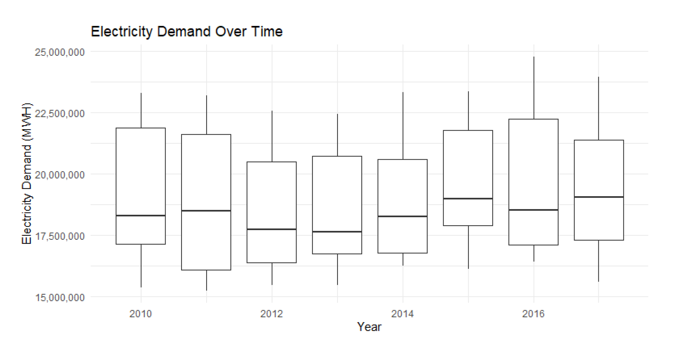
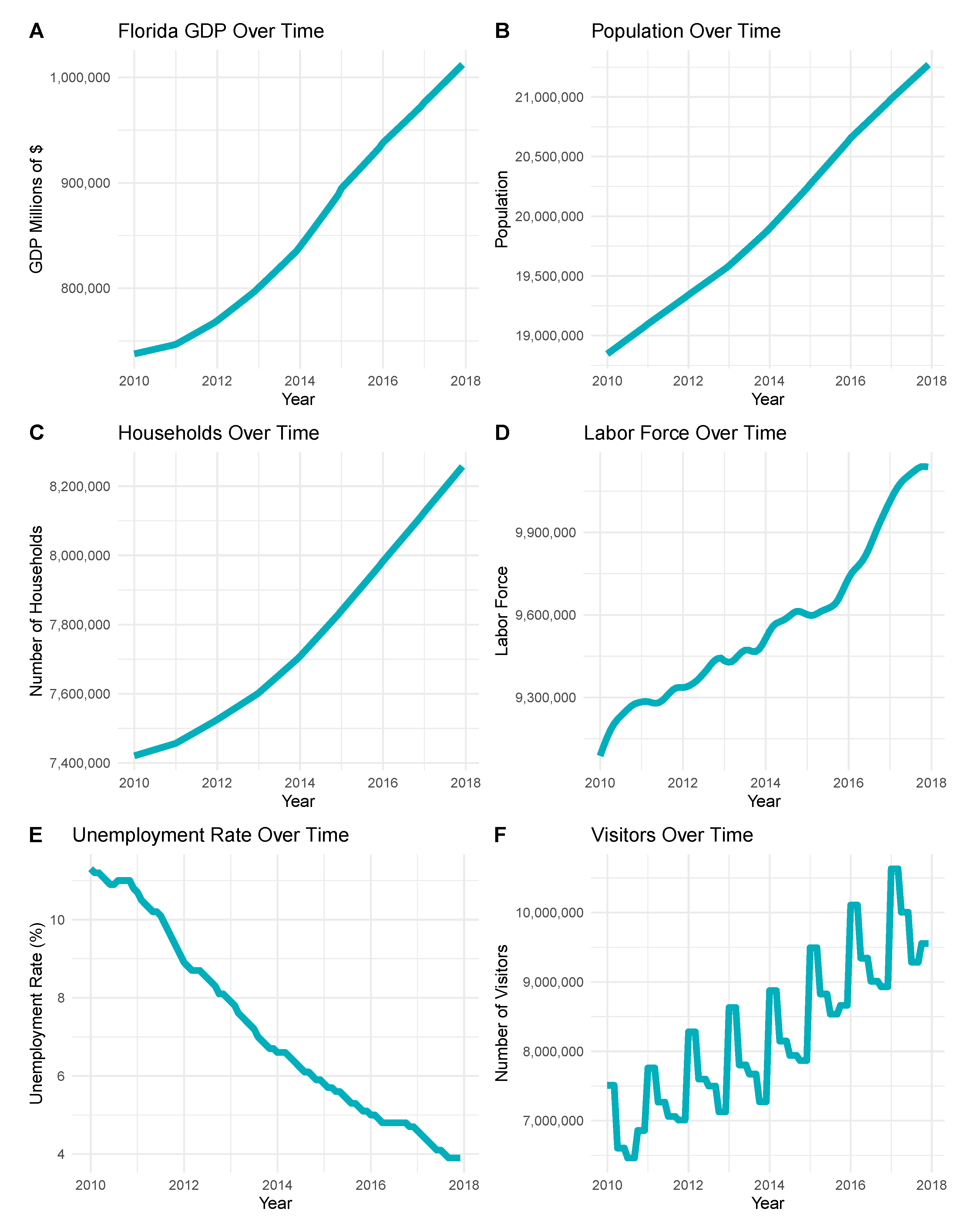
After downloading the various datasets from those sources, the data were compiled into one file. Most of the data points were broken out by month; however, a few of the variables were in the form of annual data. We determined the growth rates for these variables and then divided these rates by twelve to determine average monthly values instead of annual ones. The variables that needed to be converted from annual to monthly were: population, GDP of Florida and number of Households. We obtained historical data for the following period: January 2010 to December 2017. It was determined that there was enough data to formulate a reasonable model and achieve accurate results. The dataset is available for other researchers should they choose to replicate the results of the study or if they would like to create an extension to the study.

After all of our data collection and literature review, we proposed and applied two techniques (multiple linear regression and neural networks) to the relevant Florida electricity demand dataset. A new consensus can be added to the bank of related papers. This paper highlights three different approaches that use supervised learning and walk-forward validation. The univariant, multichannel and multihead neural networks are compared against each other as well as to the regression model. Compared to many other papers that used a Recurrent Neural Network, this paper utilizes a Convolutional Neural Network. Although CNNs are useful for classification and images, they can also be applied to time series forecasting. Even though Recurrent Neural Networks (RNNs) are able to deal with complex time series problems, it is preferable to use simpler models whenever possible. When applied to simpler tasks, RNNs are often surpassed by simpler traditional approaches, such as multilayer perceptrons.

As discussed earlier, our prediction of electricity demand requires values for economic (GDP), climatic and socio variables. GDP is a measure of the monetary value of the aggregate production of goods and services and is usually predicted based on production, expenditure and income. This economic indicator is often used by decision makers to plan economic policy and assess the future state of the economy. The forecasting of GDP has been of great interest over the years. Various classes of techniques have been used to model and forecast GDP, including parametric ones such as box and Jenkins based methodologies [18], non-linear Self-Exciting Threshold Autoregressive (SETAR) models [19], Markov switching models [20], machine learning models [21,22] and wavelet methods [23]. Reasonable GDP estimates for future years are available using the aforementioned techniques or combinations of them for countries and states. For example, the Organization for Economic Co-operation and Development (OECD) provides forecasts using a combination of model-based analyses and expert judgment [24]. Although future GDP estimates are difficult and surrounded by uncertainty, short-term (e.g., one-year-ahead) estimates have an error within 0.5%. Nevertheless, this forecast error increases as the time horizon increases but at least they offer an indication of the potential growth [25]. The forecasts are known to still be directionally accurate, and improve as the forecast horizon shortens [26].

Population growth predictions are also available for many states. For example, for the state of Florida, the Bureau of Economic and Business Research (BEBR) uses a cohort-component methodology in which births, deaths and migration are projected separately for each age–sex cohort in the population. The forecast accuracy has been determined to be approximately 3% for 5-year horizons and 4% for 10-year horizons [27]. Similarly, degree-days (HDD and CDD) are common indices used to estimate the requirement of energy for space heating and cooling, and their projected future changes have been of great interest in climate projections. For instance, the Max Planck Institute for Meteorology (MPI-M) has developed a decadal prediction system called MiKlip [28] which has improved initialization techniques using coupled ocean and atmospheric parameters. Such initialization was found to improve the accuracy of the forecasts [28]. In the context of planning for future power capacity, different GDP scenarios can be introduced and the corresponding uncertainty on demand can be further analyzed. This will help when a stochastic planning modeling approach is considered.

3. Modeling

3.1. Data Exploration

The first step consists of utilizing data exploration techniques to learn more about the data to determine the types of models that need to be formulated to solve the problem. Depending on the results, a variety of models can be used to predict the future electricity demand in Florida. The first point of interest was to determine whether electricity usage had been increasing over time in Florida. We utilized a box plot chart, as it shows us the average electricity usage per year over time. The chart showed that electricity usage had not been increasing much over the years and remained relatively stable (Figure 1).

One possible reason behind this could be that Florida has started to utilize renewable energy sources such as wind or solar, thereby reducing demand on the power grid. The electricity that is generated from renewable energy is not accounted for in electricity demand data. We were also interested in determining seasonality in our data to identify periods of high electricity usage. A box plot was also utilized in that regard, and we observe that the highest electricity use is in the summer months of June, July, August and September due to what is hypothesized to be higher average temperatures. (Figure 2A).

Due to Florida’s geographic location and unique climate compared to other states in the USA, the demand for heating systems during winter months remains low. However, the demand for air conditioning systems during the summer is fairly high due to higher temperatures. To confirm our hypothesis, a box chart of average temperatures in Florida broken down by month was created and it shows that the highest average temperatures are in June, July, August and September (Figure 2B).

The next step was to confirm our assumption of the usage of heating systems and air conditioning systems through the number of Heating Degree Days (HDD) and Cooling Degree Days (CDD). Our assumption was confirmed, and we can see that the number of Heating Degree Days is higher in the winter months (Figure 2C). We also observe the number of Cooling Degree Days and see very high numbers in the summer months (Figure 2D).

The next step in our data exploration was to determine whether Florida’s population is growing. This helped us to determine whether additional electricity demand would be needed in the future to accommodate a growing population. As observed earlier, electricity demand has been stable over the years. However, the Gross Domestic Product (GDP) of Florida has been growing over time (Figure 3A). It was found that Florida’s population has also been increasing since the beginning of 2010 and started from below 19 million, reaching over 21 million by the end of 2017 (Figure 3B). We also observe that the number of households has increased during this period from around 740,000 households to over 820,000 (Figure 3C). Labor statistics are also important in formulating a model, and we can see that the labor force has been increasing over the years as a result of a growing population (Figure 3D). The unemployment rate has been decreasing, and this indicates growth for the state of Florida (Figure 3E). Additionally, the number of visitors has been increasing over the years as well (Figure 3F). In addition, the relationship between average temperature and electricity demand was plotted and observed. As the temperature increases, electricity demand increases as expected (Figure 4).

3.2. Correlations

Another data exploration tool that can be useful in helping to define our model is to look at correlations. For our dataset, we are interested in the Pearson correlation to determine whether there is a linear relationship between variables. Our variable of interest is electricity demand, so we would like to explore the correlation between this variable and all of the other variables in the dataset. We observe that electricity demand has a strong linear relationship with the following variables: revenue (0.97), average temperature (0.81), maximum temperature (0.77), minimum temperature (0.83), and Cooling Degree Days (0.9). The remaining variables in the dataset have a weak linear relationship with electricity demand.

3.3. Multiple Regression Model

There are a variety of models that can be formulated for predicting future electricity demand in Florida. The first model that was explored was a multiple regression model that will predict electricity demand. The program R was utilized to create and assess this model. All the variables in the dataset were inserted into the regression equation to identify which predictors are significant at the 5% level. Some of the variables in the dataset were correlated; thus, multiple models were created. Previously we discussed how electricity demand has a strong correlation with revenue. Revenue was not considered in any of the models due to a multicollinearity problem. When revenue is introduced in any of the regression models, our Variance Inflation Factor (VIF) increases for all of the variables, which indicates that the model is biased and the results are untrustworthy. Due to this multicollinearity problem, revenue is not included in any of the models as a predictor. GDP was correlated with the number of visitors, number of households, population and customers (

Table 2. Regression models.

	Dependent Variable:
	Electricity_Demand
	(1)	(2)	(3)
MONTH	53,762.370 ***	84,390.860 ***	53,409.840 ***
	(19,253.940)	(20,464.910)	(19,341.870)
Cooling_Degree_Days	19,297.100 ***	19,492.030 ***	19,324.740 ***
	(554.829)	(563.787)	(557.567)
Heating_Degree_Days	18,404.850 ***	18,331.470 ***	18,482.680 ***
	(1205.019)	(1212.626)	(1213.443)
GDP_Monthly	2.972 ***
	(0.723)
Visitors		0.249 ***
		(0.064)
Population			0.354 ***
			(0.088)
Constant	9,235,152.000 ***	9,467,385.000 ***	4,693,411.000 **
	(680,154.300)	(656,067.700)	(1,798,653.000)
Observations	96	96	96
${\mathrm{R}}^2$	0.947	0.946	0.946
Adjusted ${\mathrm{R}}^2$	0.944	0.943	0.944
Residual Std. Error (df = 91)	615,575.000	620,235.300	618,154.700
F Statistic (df = 4; 91)	403.234 ***	396.857 ***	399.686 ***

* p < 0.1; ** p < 0.05; *** p < 0.01.

). Three multiple regression models were formulated, and the adjusted R-squared value was observed in order to determine which model to utilize (Table 2).

Model (1) considers only month, Cooling Degree Days (CDD), Heating Degree Days (HDD) and Gross Domestic Product (GDP) as predictors. Model (2) does not include GDP but instead includes the number of visitors, while model (3) includes population instead. Model (1) turned out to offer the best prediction ability and had the lowest standard error. Additionally, model (1) had the lowest RMSE, AIC, BIC and MAPE which indicate that it is the best regression model. (

Table 3. Regression model comparison.

		R2	RMSE	MAE	AIC
Model 1		$0.947$	$\mathrm{599,330}$	$\mathrm{445,166}$	$2838.72$
Model 2		$0.946$	$\mathrm{603,867}$	$\mathrm{452,744}$	$2840.17$
Model 3		$0.946$	$\mathrm{601,841}$	$\mathrm{448,793}$	$2839.52$
		BIC	MSE	MAPE	RSAE
Model 1		$2854.11$	$\mathrm{359,196,455,960}$	$0.024$	$0.024$
Model 2		$2855.55$	$\mathrm{364,655,802,126}$	$0.024$	$0.024$
Model 3		$2854.91$	$\mathrm{362,213,448,364}$	$0.024$	$0.024$

). All models are multiple regression models whose coefficients are given in Table 2. For example, Model 1 (column 1) is expressed as:

$$\mathrm{Electricity}\mathrm{Demand}=9,235,151+\mathrm{53,762}\mathrm{Month}+\mathrm{19,297}\mathrm{CDD}+\mathrm{18,405}\mathrm{HDD}+2.97\mathrm{GDP}$$

The assessment of this model will be discussed in Section 5.

After completing the assessment of the multiple regression model, we needed to test the accuracy of the model. Training and testing datasets were created for this purpose. The training dataset utilized the values from January 2010 to December 2015 to predict future values. The training set was used to predict the next 24 months of electricity demand, and these values will be compared to the actual demand values from January 2016 to December 2017. A regression equation is created where the actual values are the dependent variable, and the predicted values are the independent variable. This regression model assessed the accuracy of the training and testing model. Further results and assessment will be discussed in Section 5.

3.4. Convolutional Neural Network

Although Convolutional Neural Networks are widely known for their ability to analyze images, they can also be used for multi-step time series forecasting. They are able to learn features in the dataset. They work by applying filters over the dataset. CNNs have hidden layers called convolutional layers. The layers in a CNN accept an input, transform it and spit out an output. A benefit of using a CNN is that there is less preprocessing required than for other algorithms. Instead of manually coming up with the filters for the image, CNN is able to make the filters by itself by learning from the training set.

The theory behind CNN is that the filters have random weights. As the filter shifts across the dataset, these weights use matrix multiplication. We get a convolved feature that is in this case, smaller than the original, since we did not add padding. We use the maxpooling layer to keep the dominating features while decreasing the dimensions. Maxpooling keeps the highest value in the 1 × 2 square and gets rid of everything else. It also performs much better than average pooling. The dominating features allow the network to predict future electricity demand. We use the previous variables to predict the future electricity demand. The prediction is a function of past data.

$$\begin{array}{c}\hfill e_{t+1}=f^N(x_1^t,x_2^t,x_3^t,\dots ,x_n^t)\end{array}$$

The CNNs were modeled using Python. The code was based on source code from Machine Learning Mastery [29].

3.4.1. Univariant CNN

The dataset was split into training and testing datasets. The first six years were used as the training dataset and the last two years were used as the testing dataset. The univariant CNN only uses the energy usage data in order to train the model. There are two single-dimensional convolutional layers that each have 64 filters and a kernel size of 2 × 1. The ReLU activation function was used. ReLU stands for rectified linear unit and is commonly used in CNNs. It is defined as $y=max(0,x)$ which means it will only keep the positive values and the negative values become 0. ReLU takes less time to run than other activation functions and has less of a vanishing gradient problem compared to functions, such as sigmoid. ReLU is also sparsely activated which means that the model is more likely to process meaningful aspects. The single-dimensional maxpooling layer had a size 2 × 1. The model is flattened and then goes through a Long-Short-Term-Memory (LSTM) network. Lastly, it went through time-distributed dense layers. (Figure 5) The model predicts the next 24 months of energy usage by using walk-forward validation. This means the previous observations were used in order to predict the upcoming months. The CNN had 1000 epochs and a batch size of 24.

In order to measure accuracy, the Mean Squared Error, Root Mean Squared Error, Mean Absolute Error and Mean Absolute Percentage Error between the actual and predicted values were calculated. We utilized Long-Short-Term-Memory, which is an RNN structure. RNN is very useful for making predictions for time series data.

3.4.2. Multichannel CNN

The mulitchannel CNN also splits the dataset into training (first six years) and testing (last two years) datasets. This CNN differs in the additional use of all the time series variables. These include average temperature, precipitation, number of tourists, population and more. We use the same method that we used for univariant except we set up each time series variable as its own channel of input. This gives our model more information to work with and works particularly well when the output is a function of the inputs. The CNN had three one-dimensional convolutional layers with 64 filters, 64 filters and 16 filters respectively. They each had a size of 2 × 1. There were two single-dimensional maxpooling layers with a size 2 × 1. Next, there was a flattening layer followed by fully connected dense layers. The ReLU activation function was used (Figure 6).

3.4.3. Multihead CNN

The multihead CNN uses a sub-CNN model for each input variable. For each time series variable, we take the single-dimensional input that has n inputs and put it through a model that outputs a flat vector. This flat vector summarizes the features of the sequence. We can combine all the outputs for each variable through concatenation.

Each model had three single-dimensional convolutional layers that had 64 filters, 64 filters and 16 filters respectively. They each had a size of 2 × 1 and ReLU activation. There were two single-dimensional maxpooling layers that had a size of 2 × 1. There was a flattening layer. All the flattened layers were concatenated together and went through fully connected dense layers (Figure 7).

3.5. Random Forest Regression

A popular machine learning method, Random Forest regression, was explored and applied to the data in order to predict future electricity demand. The model utilized a training set and a testing set split, with the training set being the first 72 months in the dataset, January 2010 to December 2015, and the testing set being the last 24 months, January 2016 to December 2017. The program R was utilized to create this model employing the “randomForest” package. The Random Forest regression model contained 500 trees, and there were six variable nodes at each split in the decision tree of the model. The Random Forest model was assessed in order to determine whether it would be viable to include it in the comparison with the multiple regression and neural network models. The RF model had an R-squared value of 0.9249, and this is lower than both the multiple regression model and the various neural network models that are studied in this paper. Other assessment metrics that were observed were the RMSE (721,979.5), MAE (517,654) and MAPE (0.027). The values of these assessment metrics indicate that the Random Forest regression model performs worse than the multiple regression and neural network models that are studied in this paper.

4. Model Assessment

4.1. Multiple Regression Model Assessment

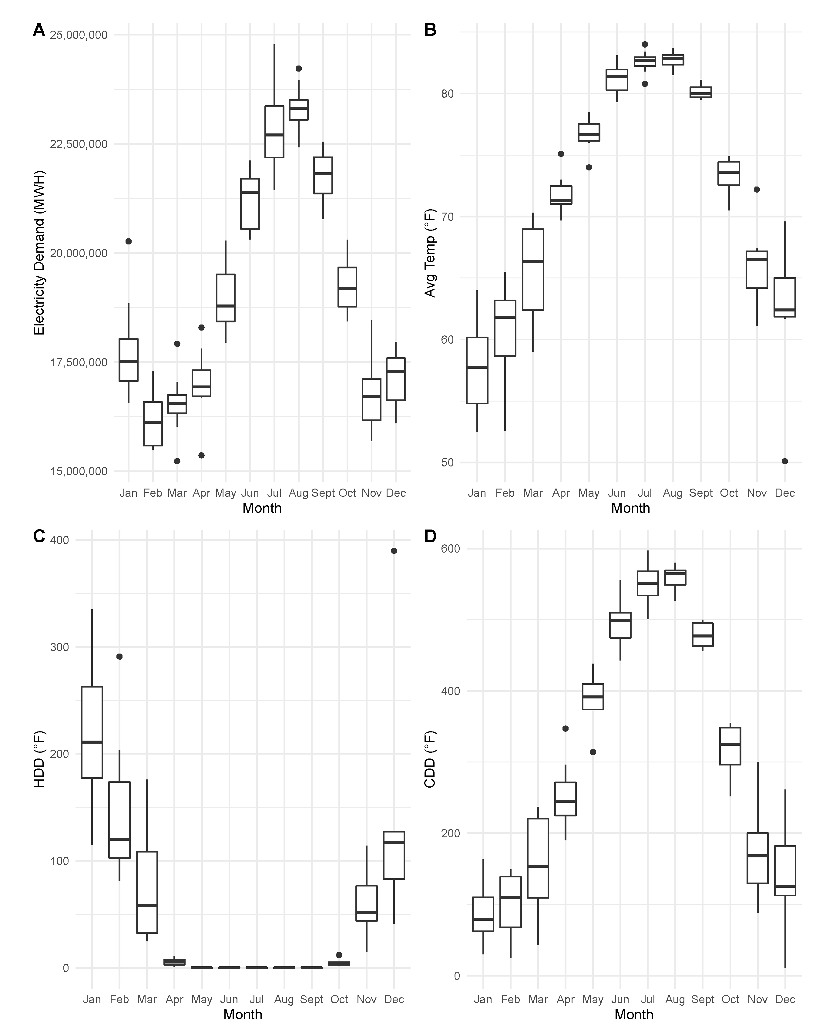
This model was found to have a larger effect size and to be statistically significant (Table 2). The interpretation of the coefficients is that for every unit increase in the independent variables, we get an increase in the dependent variable, electricity demand. For every unit increase in month, there is a 53,762 increase in electricity demand. For a unit increase in CDD, there is an increase of 19,297 units in electricity demand. For a unit increase in HDD, there is an 18,405 unit increase in electricity demand. For every unit increase in GDP, there is an increase of 2.97 units in electricity demand (Table 2). The independent variables (month, Cooling Degree Days, Heating Degree Days and GDP) that were entered into the regression equation predicted 94.4% of the variation of electricity demand—F (4,91) = 403.2, p < 0.01—and were all found to be statistically significant (Table 2).

The confidence intervals around the b weights did not include zero as a probable value, so a value of zero was not probable among the possible values. The b weight for the independent variables can be described as statistically significant. This suggests that the estimated contribution of the independent variables has sufficient precision to be retained in the specified model. The next step was to inspect the variance inflation factor for each of the predictors. The result (month = 1.1, CDD = 2.48, HDD = 2.6, GDP = 1.04) was that the VIF did not exceed 10 for any of the predictors; thus we do not have multicollinearity in our model (Table 2).

The next step was to inspect a plot of the standardized residuals against the predictor variables, and this revealed no nonlinear trends or heteroscedasticity (non-constant variance score test: chi-square = 0.0446, df = 1, p = 0.83). However, the distribution of the standardized errors did not sufficiently approximate normality (Shapiro–Wilk, W = 0.96768, p-value = 0.018). Thus, we can conclude that the results of the model should be used with care. The errors over time need to be analyzed as well to determine whether they are independent of one another. The Durbin–Watson test was utilized since the values for our dependent variable, electricity demand, were collected over time. The result was that our errors were not correlated (Durbin–Watson, D = 0.0821421, p-value = 0.112).

The results of various model assessments point to the conclusion that our model is useful and can be utilized to make predictions of future electricity demand. The next step in our analysis is to assess our training and testing regression model.

4.2. Testing Prediction Forecast

A training dataset was created which contains observations from the following time period: January 2010 to December 2015. Additionally, a testing dataset is created which contains observations from January 2016 to December 2017. This split of the dataset was that 75% was used for training, and 25% for testing. Typically, when creating a training dataset, random observations would be chosen from the original dataset. However, in this study, consecutive observations were chosen for the training set since historical data were utilized as well to account for seasonality in the data. This will allow us to get a more accurate representation of the accuracy of our predictive regression model.

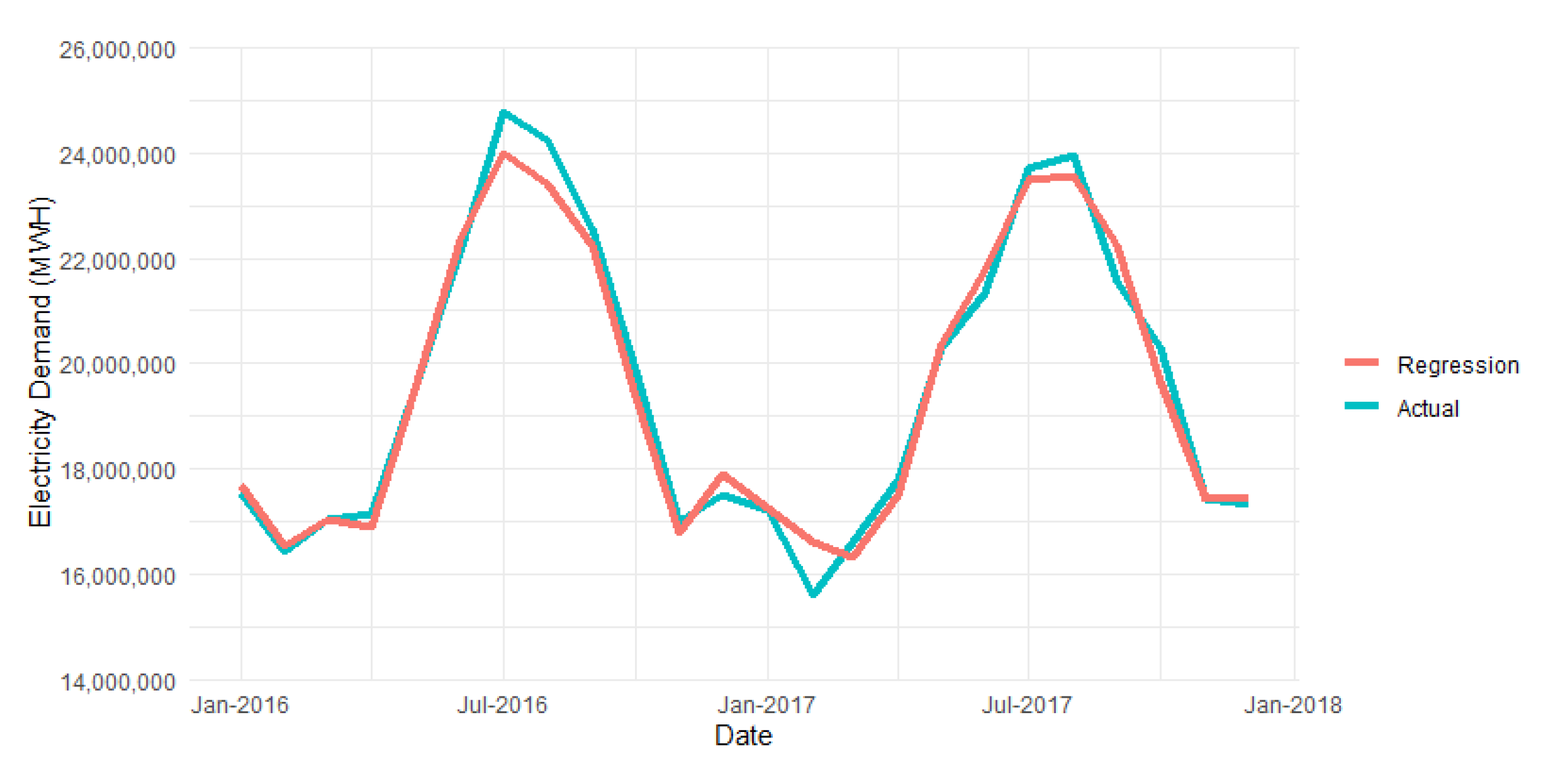
The first step was to utilize the predictive regression model and to use the training dataset. With this model, we predicted the next twenty-four monthly data points and compared them to the testing dataset. The model slightly overestimated demand in the summer months and slightly underestimated demand in the winter months (Figure 8).

The results of our data exploration indicate that the yearly average temperatures have been increasing and this can be attributed to global warming. The model will take into account this historical trend when predicting values for electricity demand.

There are a variety of methods available in order to test the accuracy of a prediction model and to test the accuracy of the predicted results versus the actual results. One of the methods is to create a regression model where the actual values are the dependent variable, and the predicted values are the independent variable (

Table 4. Regression: actual vs. predicted.

	Dependent Variable:
	Actual
Predicted	1.048 ***
	(0.033)
Constant	−865,003.600
	(646,421.800)
Observations	24
${\mathrm{R}}^2$	0.979
Adjusted ${\mathrm{R}}^2$	0.978
Residual Std. Error	425,835.000 (df = 22)
F Statistic	1014.420 *** (df = 1; 22)

* p < 0.1; ** p < 0.05; *** p < 0.01.

). This regression model will allow the assessment of the accuracy of the training and testing model.

The model was found to have a large effect size and to be statistically significant. The predicted values that were entered into the regression equation predicted 97.78% of the variation in actual values of electricity demand, F (1,22) = 1014, p < 0.01 (Table 4). The confidence intervals around the b weights did not include zero as a probable value. The b weight for the predicted values can be described as statistically significant. This suggests that the estimated contributions of the independent variables have sufficient precision to be retained in the specified model.

The next step was to inspect the plot of the standardized residuals against the predictor variables revealed, which had no nonlinear trends or heteroscedasticity. Two tests (studentized Breusch–Pagan test, and non-constant variance score test) were conducted to test for homoskedasticity, and neither was found to be significant. (BP = 0.60409, df = 1, p-value = 0.437). (Non-constant variance score test: chi-square = 0.58047, df = 1, p-value = 0.44613).

Additionally, the distribution of standardized errors was observed, and they sufficiently approximated normality (Shapiro–Wilk W = 0.93899, p-value = 0.1549). Thus, we can confirm that the results of the model are trustworthy due to the standardized errors being normally distributed. The next step was to analyze the errors over time to determine whether they were independent of one another. This is important due to the values of our dependent variable being collected over time. In this model, they are the actual values of electricity demand over time. We conducted the Durbin–Watson test, and we found that our errors were not correlated (Durbin–Watson W = −0.1276, p-value = 0.68).

The results of various model assessments point in the direction that our model is useful and can be utilized to make predictions about future electricity demand.

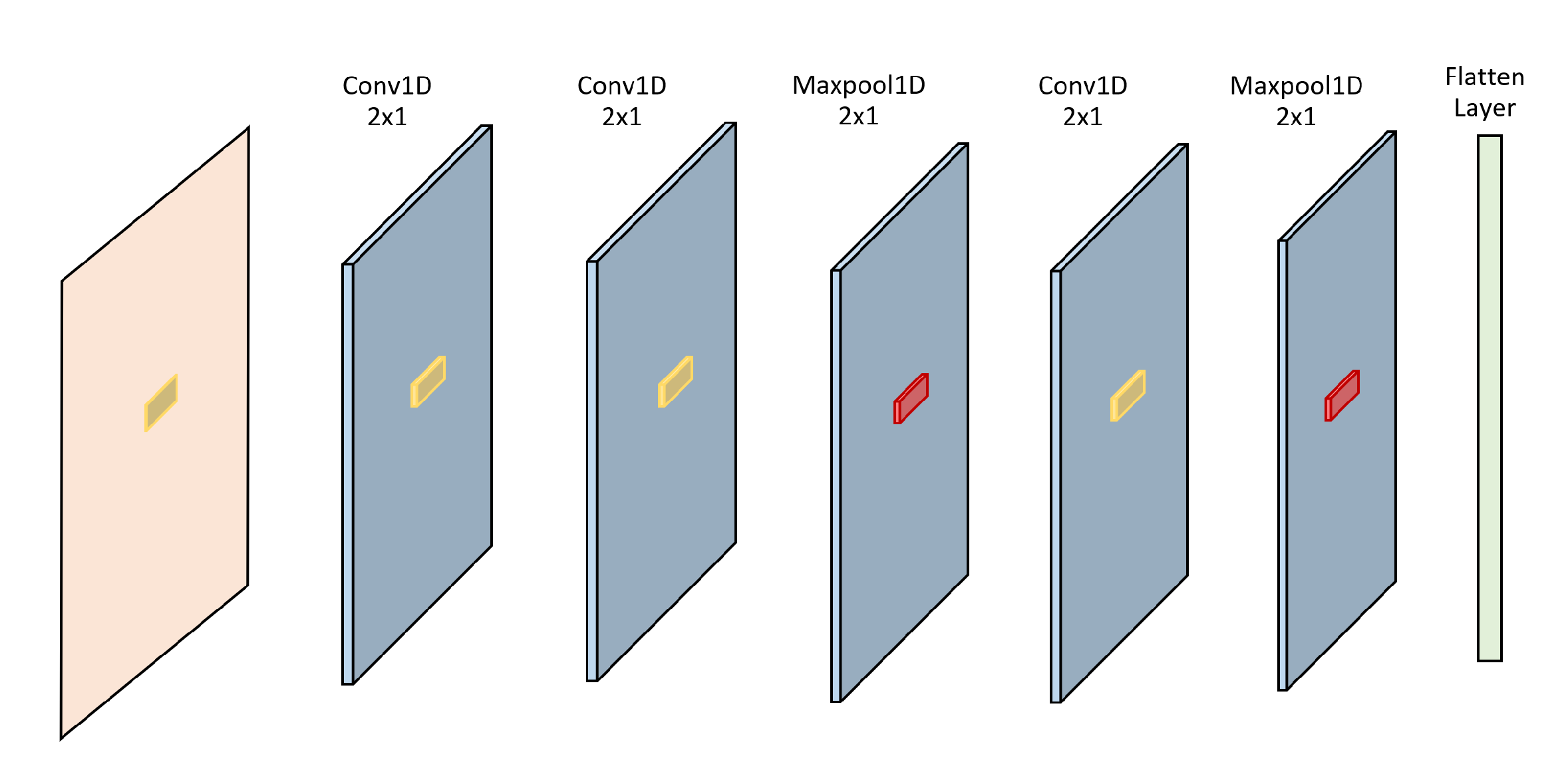
4.3. CNN

4.3.1. Univariant CNN

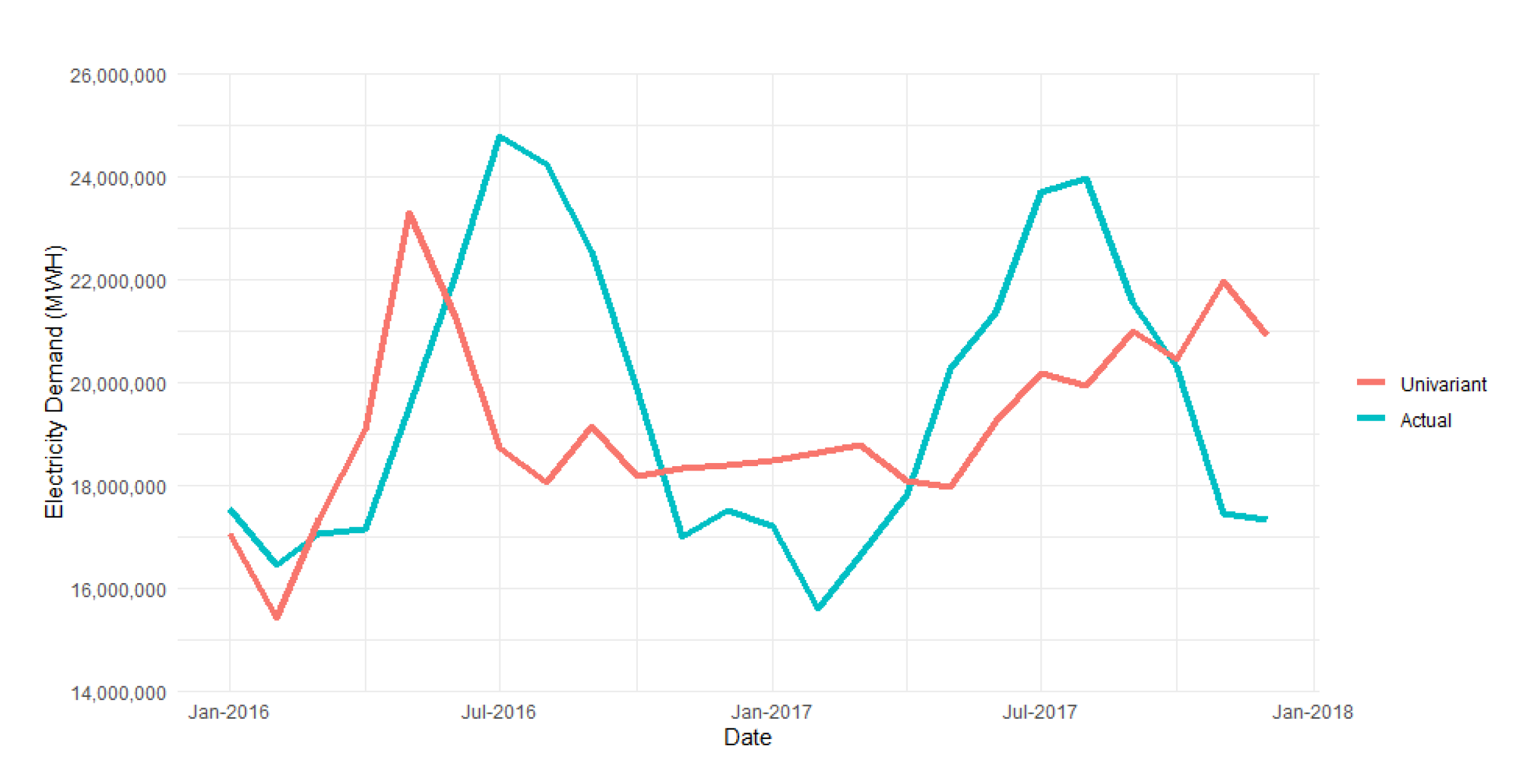
The univariant CNN model performed poorly, even with 1000 epochs. This is due to the lack of variables. The predictions were very similar to each other. The predictions varied greatly between each run. This model should not be used for electricity prediction. The MSE was 8,302,957,200,000; the RMSE was 2,881,485.2; the MAE was 2,308,165.0; and the MAPE was 0.11487670 (Figure 9).

4.3.2. Multichannel CNN

The multichannel CNN performed the best and was able to follow the dips and peaks in the data fairly well. For the summer months of the first year predicted, the model underpredicted. The years before had lower energy consumption and the years we predicted had an unusual demand spike, which the model did not catch. The model performed best with 1000 epochs. The MSE was 8,342,181,550,000; the RMSE was 584,962.87; the MAE was 474,780.29; and the MAPE was 0.025008942 (Figure 10).

4.3.3. Multihead CNN

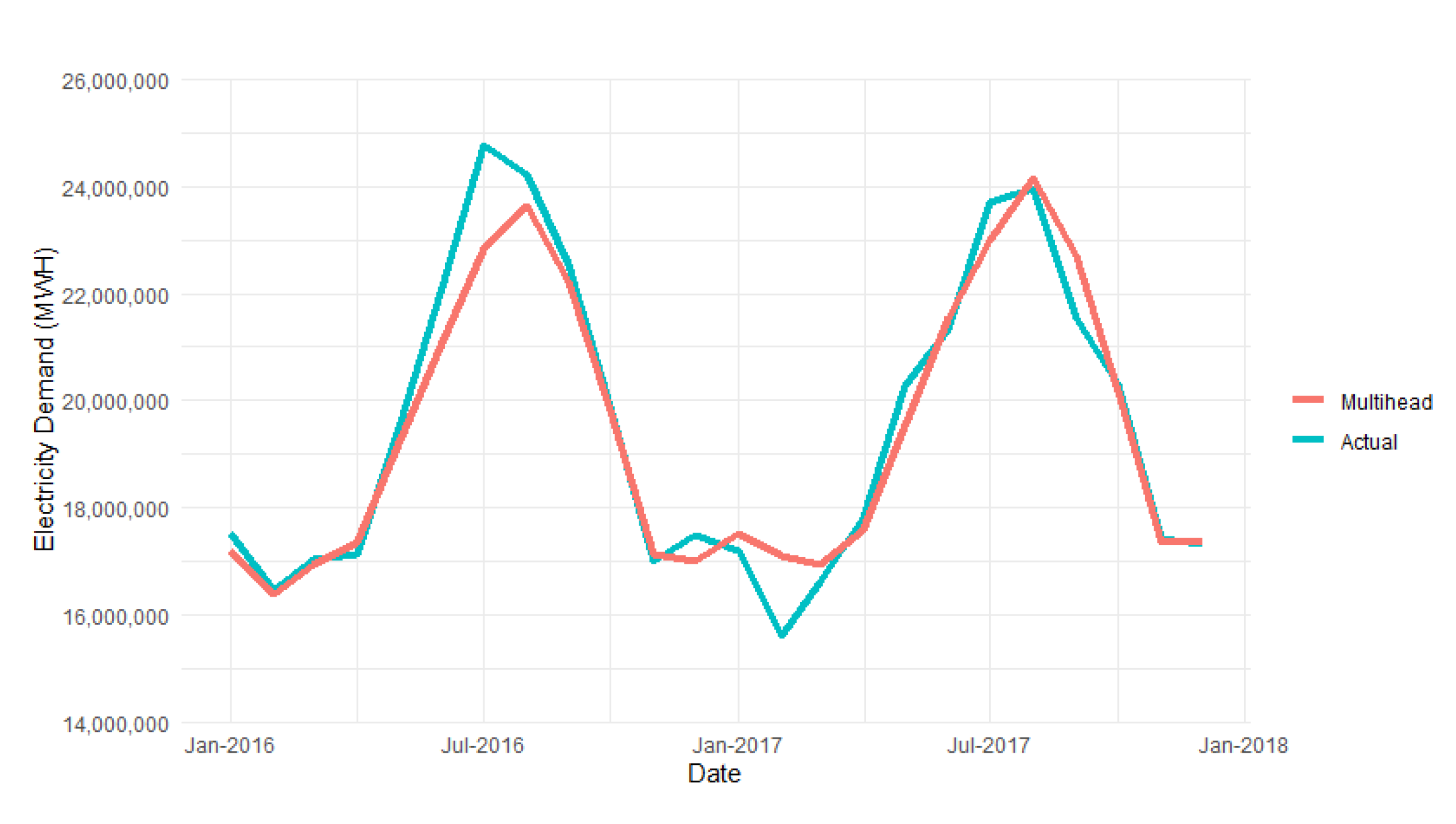
The multihead CNN was not able to predict the dips and peaks in the data. Overall the predictions followed a smoother curve, which caused it to over and underpredict often. It also took a much longer time to run and performed worse than the multichannel CNN. The best performance occurred when 1000 epochs were used. Anything above 1000 epochs caused overfitting, which resulted in worse performance. The MSE was 450,701,240,000; the RMSE was 671,342.86; the MAE was 466,385.17; and the MAPE was 0.023179748 (Figure 11).

4.4. CNN vs. Regression Comparison

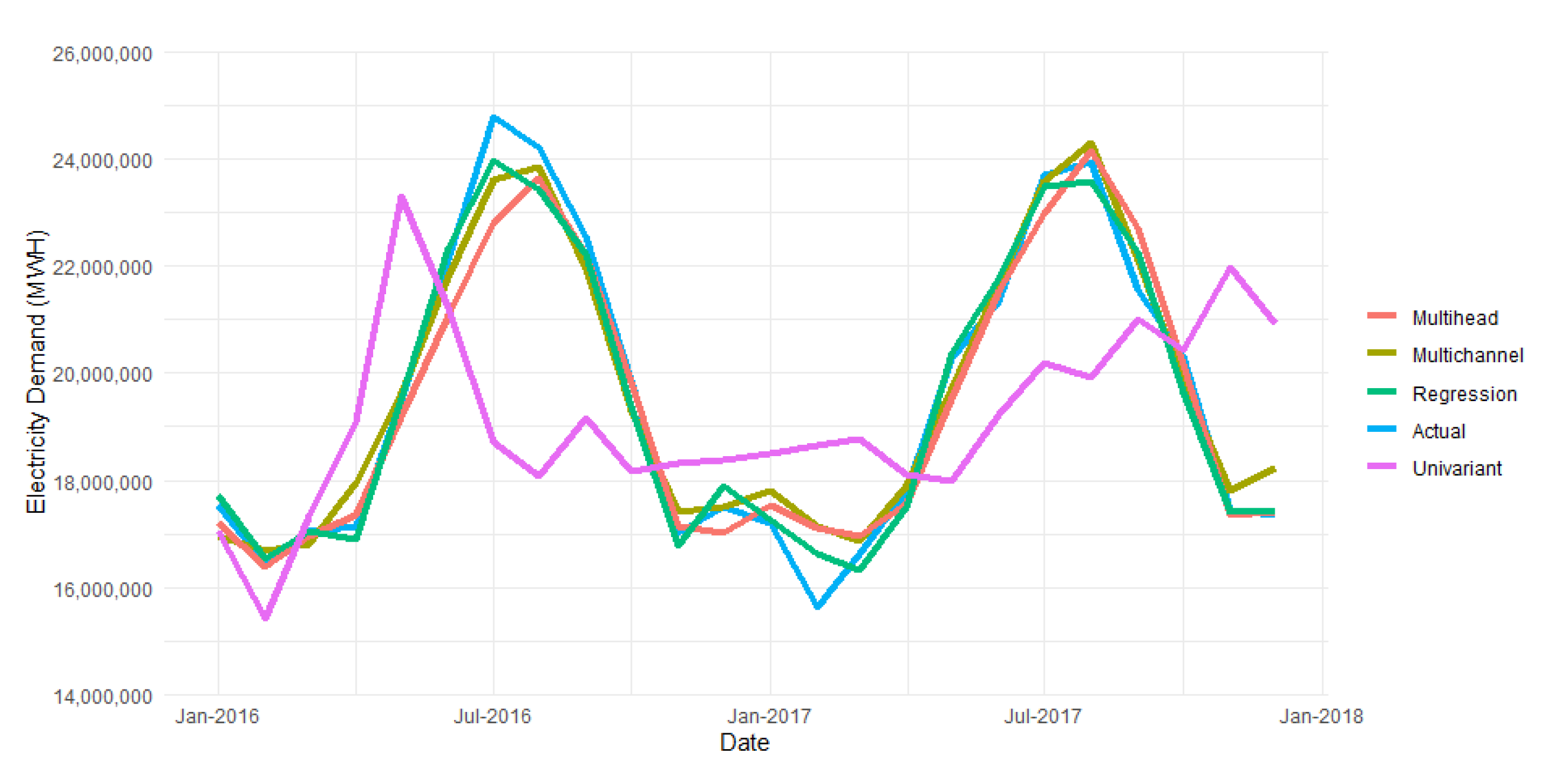
Various model assessment metrics were utilized to assess the accuracy of the regression models and the neural network models. These assessment metrics allow us to compare the models with each other in order to determine which model best predicts electricity demand. The following are used to assess the accuracy of each model: min-max accuracy, R-squared, Root Mean Squared Error (RMSE), Mean Absolute Error (MAE), AIC, BIC, Mean Squared Error (MSE), Mean Absolute Percentage Error (MAPE) and Robust Small Area Estimation (RSAE). When observing the min-max accuracy of all the models (

Table 5. Overall model results.

	Min.Max Accuracy	R2	RMSE	MAE	AIC	BIC
Regression Model	$0.977$	$0.947$	$\mathrm{599,330}$	$\mathrm{445,166.800}$	$2838.721$	$2854.107$
Multihead	$0.979$	$0.95$	$\mathrm{671,342}$	$\mathrm{432,002}$	$714.84$	$718.38$
Multichannel	$0.978$	$0.963$	$\mathrm{584,962}$	$\mathrm{438,206}$	$707.49$	$711.02$
Univariant	$0.889$	$0.071$	$\mathrm{2,881,485}$	$\mathrm{2,356,897}$	$784.89$	$788.43$
	MSE	MAPE	RSAE
Regression Model	$\mathrm{359,196,455,960}$	$0.024$	$0.023$
Multihead	$\mathrm{450,701,238,904.58}$	$0.02318$	$0.030$
Multichannel	$\mathrm{342,181,554,643.63}$	$0.02501$	$0.027$
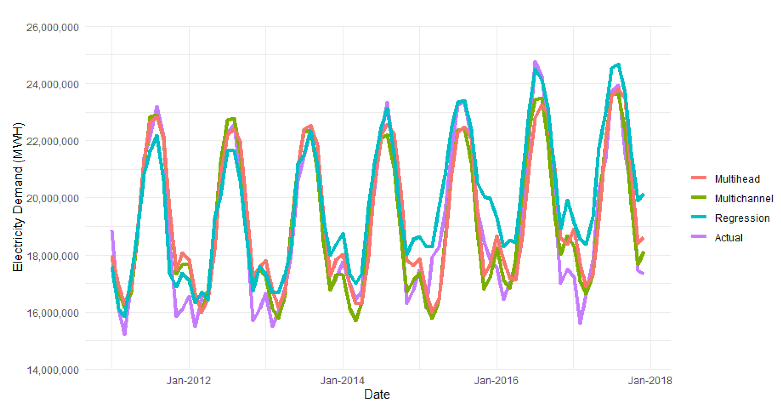
Univariant	$\mathrm{8,302,957,215,341.45}$	$0.11488$	$0.120$

), the model that performs the best is the multichannel CNN model that utilizes the training and testing dataset with an accuracy of 97.8%. This model also has the highest R-squared value of 0.963. The next model assessments of interest are AIC and BIC. The lower the values for these, the better the model is at predicting electricity demand. The multichannel CNN model with the training and testing dataset has the lowest values for AIC and BIC. The next step was to observe the MSEs of all the models, and again the multichannel CNN model with the training and testing dataset has the lowest MSE. The last model assessment variable to observe is MAPE, and again, the multichannel CNN model with the training and testing dataset had the lowest MAPE. When plotting predictions of all the models versus the actual electricity demand, the multichannel CNN model preforms best, as it has the closest trend to the actual electricity demand (Figure 12).

4.5. Further Experimentation

The multichannel CNN performed the best out of all the CNNs and only performed a little better than the regression model. The same models were further tested on a much larger dataset that started in 1990. The dataset was split into 75% testing and 25% training datasets and was set up the same way as the original dataset (

Table 6. Overall model results with the 1990 dataset.

	MSE	RMSE	MAE	MAPE
Regression Model	$\mathrm{1,398,430,500,000}$	$\mathrm{1,182,552.5}$	$\mathrm{956,231.70}$	$0.052918386$
Multihead	$\mathrm{917,534,200,000}$	$\mathrm{957,880.06}$	$\mathrm{773,288.23}$	$0.042361177$
Multichannel	$\mathrm{642,311,040,000}$	$\mathrm{801,443.10}$	$\mathrm{659,891.61}$	$0.035784574$

). The results indicated that the original experiment for the mutichannel and multihead CNN did not perform as well as we thought it would, since it did not have a sufficiently sized dataset. The multichannel and multihead CNNs performed much better than the regression model when tested with the new enhanced dataset (Figure 13).

5. Future Work and Limitations

The results of the models proposed in the paper are favorable and can be utilized to predict electricity demand for the state of Florida; however, there is room for improvement. One of the improvements that can be made when building the model is collecting more historical data. This paper only utilized seven years of data, from 2010 to 2017. In the future, a new model could be developed which uses many more years of historical data and this would definitely help to improve the model accuracy of both regression and neural network models. Other improvements to the model can be in the form of collecting data on other variables to determine whether they have an effect on electricity demand prediction. A variety of case studies can be conducted depending on the variables that are collected. Climate variables can be considered, such as wind speed, evaporation or humidity. The incorporation of economic variables in the model can also be considered to determine whether they have any effects on electricity demand. Another area to consider would be Electric Vehicles. Due to the emergence of Electric Vehicles and consumers becoming more environmentally conscious, the demand for electricity to charge these vehicles will increase. Thus, collecting data on the number of vehicles in the market and data from charging stations would be a good start. The last variable to take into consideration would be to study the effects of adverse events on electricity demand in the state of Florida, mainly the effects of hurricanes. Hurricanes are becoming more prevalent due to climate change and their effects should be studied. Another area to take into consideration would be electricity use in various sectors, industrial, commercial and residential, and studying their effect on the overall use of electricity in Florida.

6. Conclusions

This paper considered two classes of models to predict electricity demand in the state of Florida. A variety of variables that included economic, social and climate variables were collected and introduced into the models. The time period of interest was 2010 to 2017 for all of the data that were collected. The first model that was proposed was a multiple linear regression model and this model was 97.7% accurate in predicting electricity demand. The significant variables, month, Cooling Degree Days (CDD), Heating Degree Days (HDD) and GDP explained 94.7% of the variation in electricity demand. Various model assessments were utilized and they pointed to the direction that our model is useful and can be utilized to make predictions for future electricity demand.

Using Root Mean Squared Error, we are able to investigate how far the predicted energy usage was compared to the actual energy usage. We simulated our model five times and found the average of the RMSE. When comparing the neural networks, it was clear from looking at the statistics that the RMSE was worse when we used univariant CNN. The multihead CNN performed better than the univariant CNN and the multichannel CNN performed the best. It seems that the added variables help the model make more accurate predictions. The univariant performed very poorly and the results were erratic.

All models underpredicted the first summer peak. This could be because this particular summer had unusually high electricity demand compared to the other summers of previous years. The neural network models were tested on only the significant variables, according to the regression model. These variables included month, Cooling Degree Days, Heating Degree Days and GDP. The model performed worse compared to using all of the variables in the original dataset.

When comparing the neural networks to the linear regression model, it was clear that the multichannel and multihead CNNs performed better. When the dataset size was increased, both the multichannel and multihead CNNs outperformed the linear regression to a larger extent compared to the original dataset. The multichannel CNN had a prediction accuracy of 97.8%, which was 0.1% more accuracy than the multiple linear regression model when predicting future electricity demand.