Occupancy Prediction Using Differential Evolution Online Sequential Extreme Learning Machine Model

1
Department of Building Energetics, Faculty of Environmental Engineering, Vilnius Gediminas Technical University, 10223 Vilnius, Lithuania
2
Department of Construction Management and Real Estate, Faculty of Civil Engineering, Vilnius Gediminas Technical University, 10223 Vilnius, Lithuania
3
Department of Business Technologies and Entrepreneurship, Faculty of Business Management, Vilnius Gediminas Technical University, 10223 Vilnius, Lithuania
*
Author to whom correspondence should be addressed.
Energies 2020, 13(15), 4033; https://0-doi-org.brum.beds.ac.uk/10.3390/en13154033
Submission received: 15 July 2020
/
Revised: 30 July 2020
/
Accepted: 31 July 2020
/
Published: 4 August 2020
(This article belongs to the Section A: Sustainable Energy)
Abstract
:Despite increasing energy efficiency requirements, the full potential of energy efficiency is still unlocked; many buildings in the EU tend to consume more energy than predicted. Gathering data and developing models to predict occupants’ behaviour is seen as the next frontier in sustainable design. Measurements in the analysed open-space office showed accordingly 3.5 and 2.7 times lower occupancy compared to the ones given by DesignBuilder’s and EN 16798-1. This proves that proposed occupancy patterns are only suitable for typical open-space offices. The results of the previous studies and proposed occupancy prediction models have limited applications and limited accuracies. In this paper, the hybrid differential evolution online sequential extreme learning machine (DE-OSELM) model was applied for building occupants’ presence prediction in open-space office. The model was not previously applied in this area of research. It was found that prediction using experimentally gained indoor and outdoor parameters for the whole analysed period resulted in a correlation coefficient R2 = 0.72. The best correlation was found with indoor CO2 concentration—R2 = 0.71 for the analysed period. It was concluded that a 4 week measurement period was sufficient for the prediction of the building’s occupancy and that DE-OSELM is a fast and reliable model suitable for this purpose.
1. Introduction
Despite increasing energy efficiency requirements for buildings across the EU, the full potential of energy efficiency is still unlocked. The significant progress has been made on a legislative and political level, but still much has to be done to change the final users’ energy consumption-related behaviour. Together with policy developments, building occupants’ behaviour plays an important role in achieving ambitious goals, as new consumption opportunities may arise because of energy efficiency gains, which may impair efforts to reduce overall energy consumption.
The building sector remains one of the most energy intensive sectors, producing about one-third of total global greenhouse emissions in the EU [1]. During the design phase of the building, national regulations or standards like LEED or BREEAM usually dictate how much consideration must be given to the energy performance; ratings for energy performance certificates are produced to meet the requirements. However, there is significant evidence that buildings, when they are constructed, do not perform as was predicted during the design phase [2,3]. According to the platform CarbonBuzz [4], the initiative of the collaboration between the Royal Institute of British Architects (RIBA) and the Chartered Institution of Building Services Engineers (CIBSE), many buildings across the EU tend to consume 1.5 to 2.5 times more energy than predicted. The less-than-expected operational energy savings astonish investors; meanwhile, occupants suffer from poor indoor comfort or air quality. This is called the performance gap between the expected and actual performance (in terms of energy consumption and indoor environment). Some researchers blame energy simulations that fail to capture how buildings actually work, but a number of factors could be responsible for this discrepancy.
Energy simulation is a powerful tool, enabling to minimize the energy performance gap, but its results strongly depend on assumptions. Simulation tools use as input data climatic data, physical properties of the building envelope and technical properties of the engineering systems. Meanwhile, the impact of occupancy behaviour is only estimated through default or standard schedules [5]. Peper and Feist [6] estimated that the occupants’ influence on energy consumption is ±50%. Therefore, the influence of occupants’ behaviour should not be underestimated. However, a lack of occupancy monitoring and feedback means that problems are rarely identified, occupancy behaviour (OB) is not corrected and lessons are not learned for future projects.
Currently, the understanding of the importance of OB in the building’s design, operation and modernization stages are very limited, thus resulting in significant performance gaps when comparing the simulated vs. actual building’s performance [7]. Therefore, gathering data and developing models to predict energy performance, and change building operation, as well as OB, is the next frontier in sustainable design.
When analysing OB, it is important to understand that occupants may influence energy consumption through their passive and active behaviour [5]. Passive behaviour is mainly related to the presence of the occupants and related metabolic heat gains, which influence the thermal balance of the building and indoor air quality. The passive influence is forecasted considering the occupancy profiles, and it is important in a building’s design phase for accurate energy demand predictions, and in the operation phase, for the heating, ventilation and air conditioning (HVAC) system performance optimisation. Meanwhile, the active occupants’ behaviour is understood as occupants’ actions, which influence the energy consumption of the building. These actions are targeted to achieve the desired indoor comfort level and include opening and closing windows, adjusting window blinds, changing thermostat settings, controlling the lighting system, etc. Besides, occupants can influence buildings’ electricity consumption by the specific use of electrical devices, and this is more related to the behavioural aspects. Various actions often cause an undesired increase in operational energy consumption. Active behaviour is complicated and difficult to predict as it depends on many types of factors including individual (e.g., psychological, physiological), social-personal (e.g., education, knowledge, life-style), economic (e.g., price of energy, incomes), cultural, climatic, and architectural.
The field of research dealing with the understanding and simulation of OB in the built environments is evolving rapidly [8], and a clearer insight towards understanding the impacts of OB on energy consumption has been provided. However, several gaps in OB research are remaining, however [9], developed OB models resulting from both deterministic and probabilistic methods present a dependency on the data set used in their development [10]. Particularly, the translation and integration of the results of performed studies into building energy simulation tools to reduce the performance gap is seen as a significant research challenge in the area. Furthermore, future investigations about the inter-relationship between different OBs are needed, to generate more realistic assumptions in building energy performance predictions [5]. A lack of scientific and robust models to define and simulate energy-related OB in buildings was also indicated by the International Energy Agency [7]. A literature analysis revealed that occupancy profiles are predicted in many studies by using different methods, but to date the application of the methods was limited to low reliability. Recent studies show that to predict occupancy behaviour in buildings, some authors make attempts to apply promising extreme learning machine methods [11,12,13,14,15]. For example, Chen et al. (2016) [13] applied an extreme learning machine (ELM)-based wrapper method to select the best feature set of environmental parameters and proposed a fusion framework for occupancy estimation in office buildings. Masood et al. (2018) [15] for indoor occupancy estimation proposed a novel technique called the hybrid feature-scaled extreme learning machine (HFS-ELM). Chen et al. (2019) [16] proposed a novel ensemble ELM algorithm for human activity recognition using smartphone sensors. For the prediction of occupancy level and energy consumption in an office building, Wei et al. (2019) [17] applied blind system identification and neural networks. Jiang et al. (2020) [18] proposed a model based on a novel ensemble extreme learning machine technique that can estimate the occupancy level from carbon dioxide concentration. The results obtained in validations demonstrate that forecasting models that include extreme learning machine show high accuracy. Such data-driven approaches have become popular due to their ability to uncover statistical patterns without the intervention of experts [19].
The goal of this paper is to test—for the first time—the applicability of the hybrid differential evolution online sequential extreme learning machine (DE-OSELM) method for occupancy prediction.
2. Previous Related Work
The prediction of building occupants’ behaviour at the early design stage is becoming increasingly more challenging due to the complexity of the built environments in terms of size, spatial solutions, many functions, and the variety of user types [20,21,22]. A review of previous studies on building–user interactions and occupancy profile predictions revealed the evolving trend in the application of prediction methodologies, measuring periods and measured variables. Some observations are presented in Table 1.
The varying behaviour of occupants results in different energy usage patterns. Occupant behaviour (like presence, activity patterns, etc.) is usually included in the set of parameters related to building performance assessment [7,23]. This set also includes climate data, building characteristics (like building orientation, area, physical properties of building materials, etc.), and data on building service systems, indoor thermal comfort and air quality. Most studies related to the measurement and modelling of occupancy patterns usually focus on the simulation of occupant presence and behaviour, like the time the user starts working, finishes work, goes to lunch, and returns in the afternoon [24,25,26,27,28]. Some studies presented algorithms for occupancy number detection based on the analysis of environmental data (i.e., CO2, CO, total volatile organic compounds (TVOC), relative humidity (RH), outside temperature, dew point, small particulates, motion, acoustics) captured from sensors [29,30,31,32,33]. Most often, studies combine the approaches of environmental data measurements, energy consumption data and the observations of occupants’ presence [34,35]. For the modelling of personalized occupancy profiles, the study [36] observed the door open/closed status additionally to the environmental data. For office activity recognition, the study [37] explored per-desk passive infrared (PIR) sensors and power plug meters. The heat transferred to the common space together with the presence of occupants and outdoor air, and ground temperatures were observed with the aim to reduce energy consumption at the beginning of occupancy and make the best possible use of stored thermal energy [38,39]. The variables of time spent in the room and the switching on and off of the lights were used for the modelling of occupancy and building users’ behaviour to predict the energy consumption [40]. The techniques based on Wi-Fi signals from consumer devices and bluetooth low energy (BLE)-based real-time locating systems were also used to detect the presence of occupants [41,42,43,44]. Recently, the networks of interconnected and mutually interactive devices to exchange information with each other were used for the indirect monitoring of occupancy and to collect the data on CO2, temperature, and relative humidity [45].
For the analysis of the dynamic relationships between human activities and built environments, various simulation approaches are proposed. Data-driven approaches to predict the occupants’ presence and behaviour in open office spaces and to analyse indoor comfort and energy consumption are most common if large data sets are available [20]. The algorithms based on approaches based on Markov chain were used in most of the analysed studies for simulating occupant presence or activities [24,25,38,39,40,46]. Some other models, rarely used, include the Monte Carlo [35], regression and time-series models [36], Dynamic Markov Time-Window Inference (DMTWI), Auto-Regressive Moving Average (ARMA) and Support Vector Regression (SVR) models [42], agent-based models (ABM) [47], Gaussian approach [46,48], and artificial neural networks (ANN) [29,30,49,50]. New approaches like extreme learning machine (ELM) and its modifications [11,12,13,14,15], narrative-based modelling and multi-criteria analysis [20], have also been used recently.
Most studies emphasize the need for a more suitable and accurate occupancy prediction model. Under constant loads, such as a residential building, energy consumption follows a certain pattern; thus, the variability in energy consumption is not volatile. On the contrary, buildings with varying occupancy levels, such as mixed-use buildings, have a changing pattern in their energy demands. Such high fluctuation leads to poor prediction accuracy [21]. The models that are currently proposed have limitations; they cover limited measurement periods; moreover, they do not assess the seasonal differences among the different behaviour scenarios and they cannot fully reflect the stochastic nature of the occupants’ behaviours.
3. Methodology
The methodology applied in the paper consisted of two main steps:
- Experimental research of the occupancy and physical indoor and outdoor parameters in the open-space office building was conducted. Experimentally defined occupancy profiles were generated. Three different cases—DesignBuilder default, standard EN 16798-1 and actual measured—were simulated and compared to investigate the influence of occupants’ schedules assumptions on energy consumption in an open-space office.
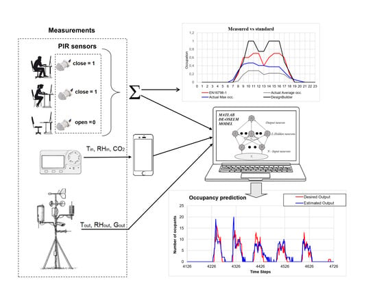
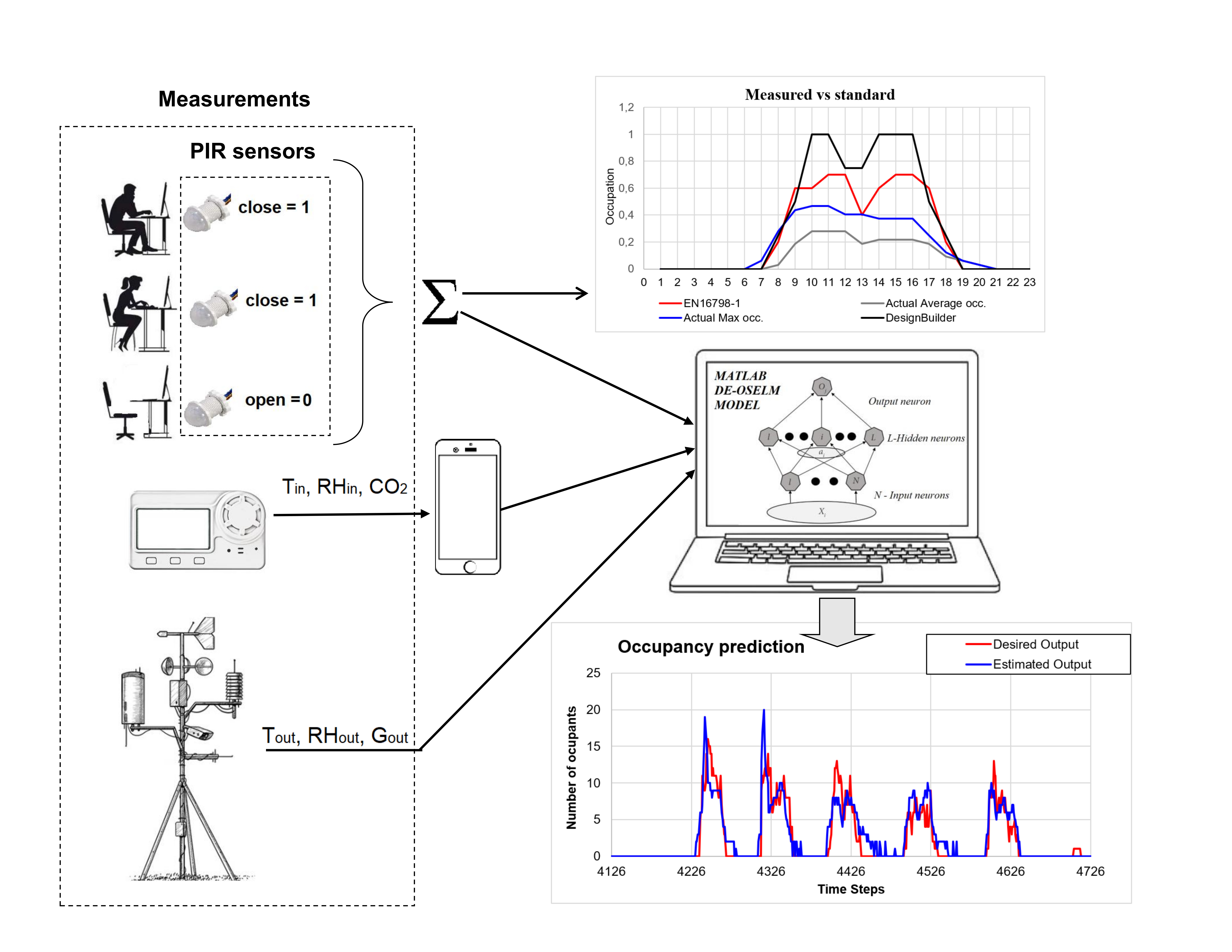
- A model was created with MATLAB, which could forecast occupancy presence. The hybrid differential evolution online sequential extreme learning machine (DE-OSELM) method was applied for the first time for the prediction of occupancy. In the used model, a single-hidden layer feedforward neural network (SLFNN) was constructed, as well as a neural network architecture consisting of a number of inputs, transfer function type, and a number of hidden neurons in the hidden layer. The ELM modelling consisted of 3 stages: training, testing and validation. Data from the entire aggregated set were divided into three parts, of which a random arrangement was made for each of the three stages. A random breakdown of the data avoided simultaneous unpredictable coincidences. To optimise the training stage, the differential evolution (DE) algorithm was employed. Before the training stage, the hyperparameters were defined. In machine learning, a hyperparameter is a parameter whose value is used to control the training process. Usually, these hyperparameters are determined from accumulated experience (empirically) by manual testing or performing a detailed search. The evolutionary optimization algorithms were used to find a set of hyperparameter values. The DE algorithm improved the data by one generation, so the source data were classified. Classified data were further used in the ELM training stage. The mathematical expression of the methodology was described below.
3.1. Experimental Research
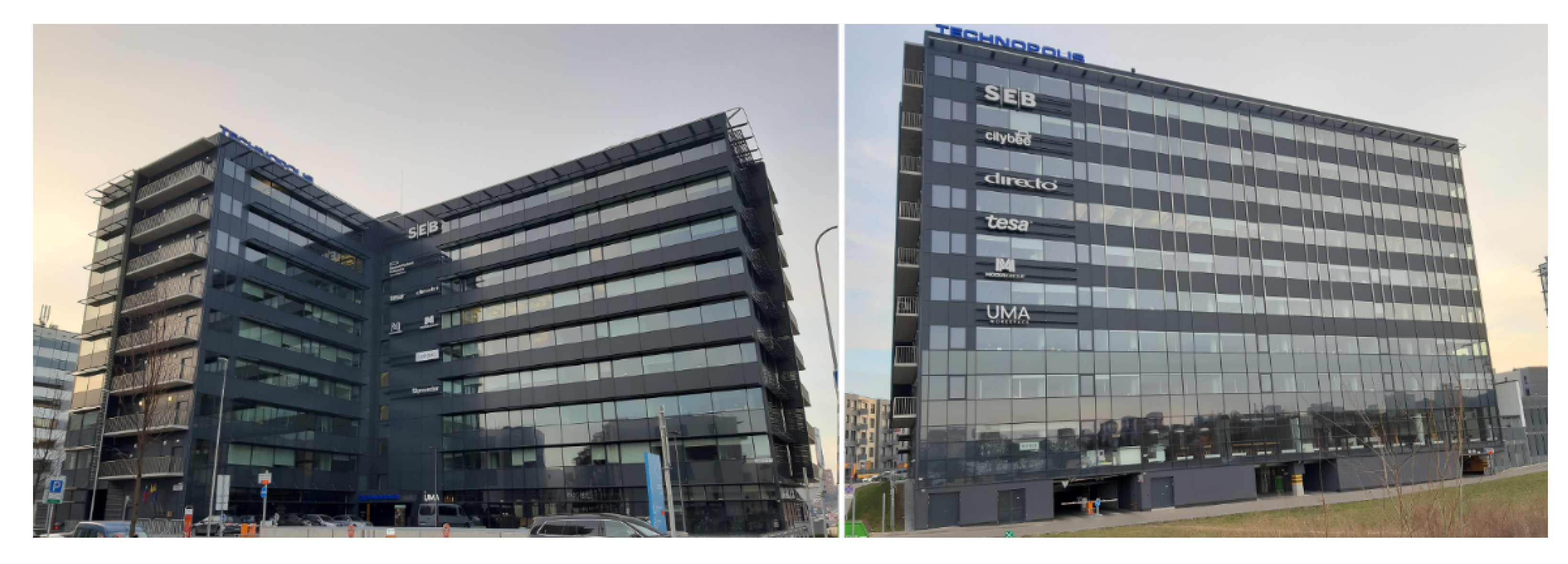
For the actual occupancy profiles research, a building with open-space offices and mobile work stations (computer tables are not assigned to employees; they occupy the one, which is not occupied when they arrive) was selected. The building was energy-efficient and sustainable, LEED GOLD-certified, thus assuming that it provides better working conditions for the users. Basic data related to the building are presented in Table 2 and the building facades are shown in Figure 1.
The comfort in the building during the heating season is maintained by the system of radiators, and during the cooling season, by active chilled beams (combined with ventilation). Thermostats installed 2.5 m above the floor adjust the room air temperature for heating or cooling. Thermostats are centrally controlled from the main control system (BMS—building management system), so occupants have no possibility of adjusting the parameters of the indoor climate. Fresh air is supplied to the premises through active chilled beams, and the airflow is constant during the occupied hours. Ventilation and cooling systems are activated from 06:30 to 19:00. The heating system is always activated during the heating season.
One of the most important measurement parameters in this study was the presence of people, which influences changes in the energy consumption of indoor climate systems. Indoor occupancy or workplace occupancy can be observed with devices like 3D depth cameras, which have been extensively studied by Diraco et al. [51]. Three-dimensional cameras can capture people’s presence and behaviour with great accuracy. Another investigated method is PIR (passive infrared sensor) and noise sensors based or VOC (volatile organic compounds), CO2 (carbon dioxide), and relative humidity, but these only detect the presence/absence of people indoors [52]. CO2 VOC, RH (relative humidity) are sensors that record the increase in the measured parameters compared to the normal parameters, thus referencing to the presence in the room. This is not an accurate method of detecting occupancy, because it indicates that the room is occupied, but does not provide the information on the exact number of occupants.
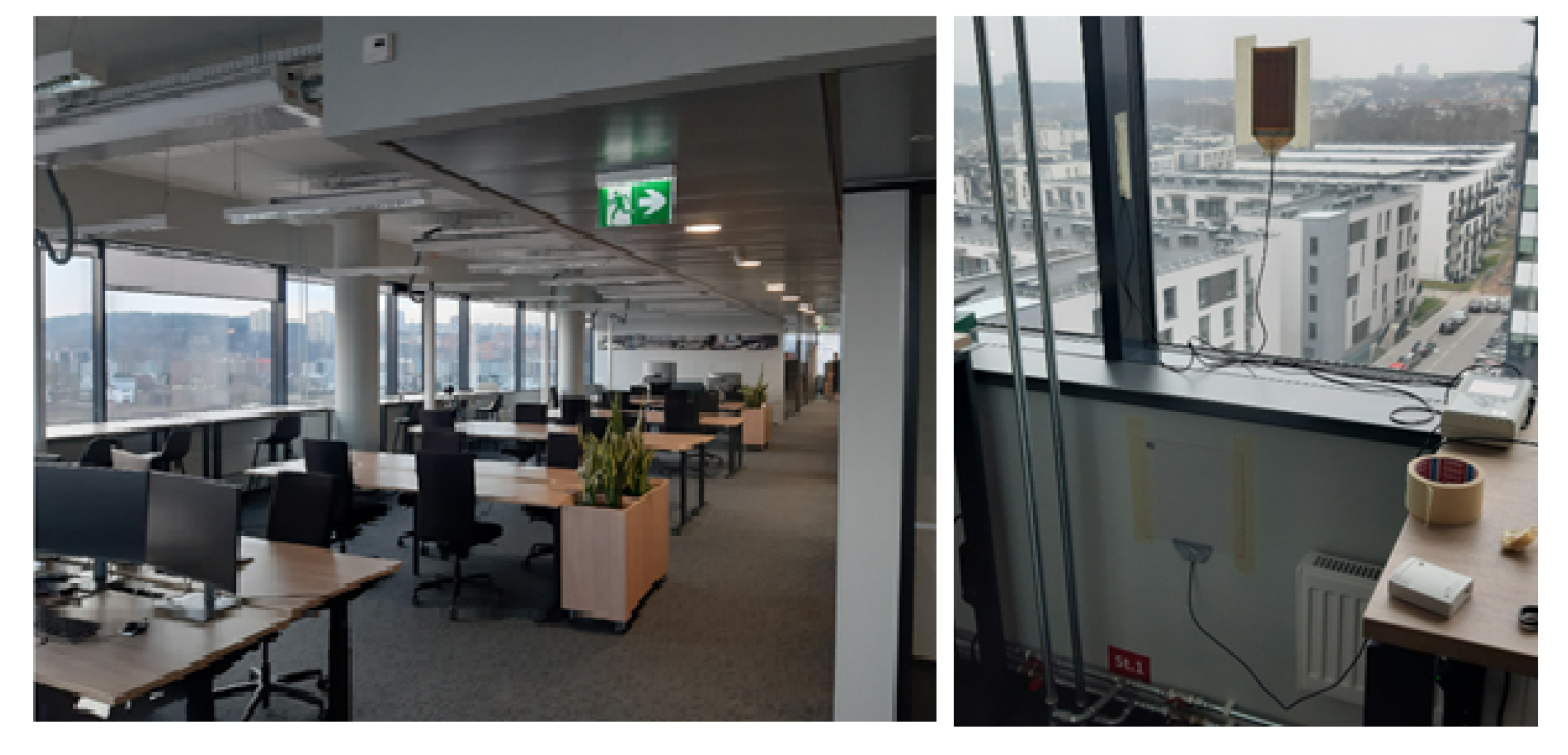
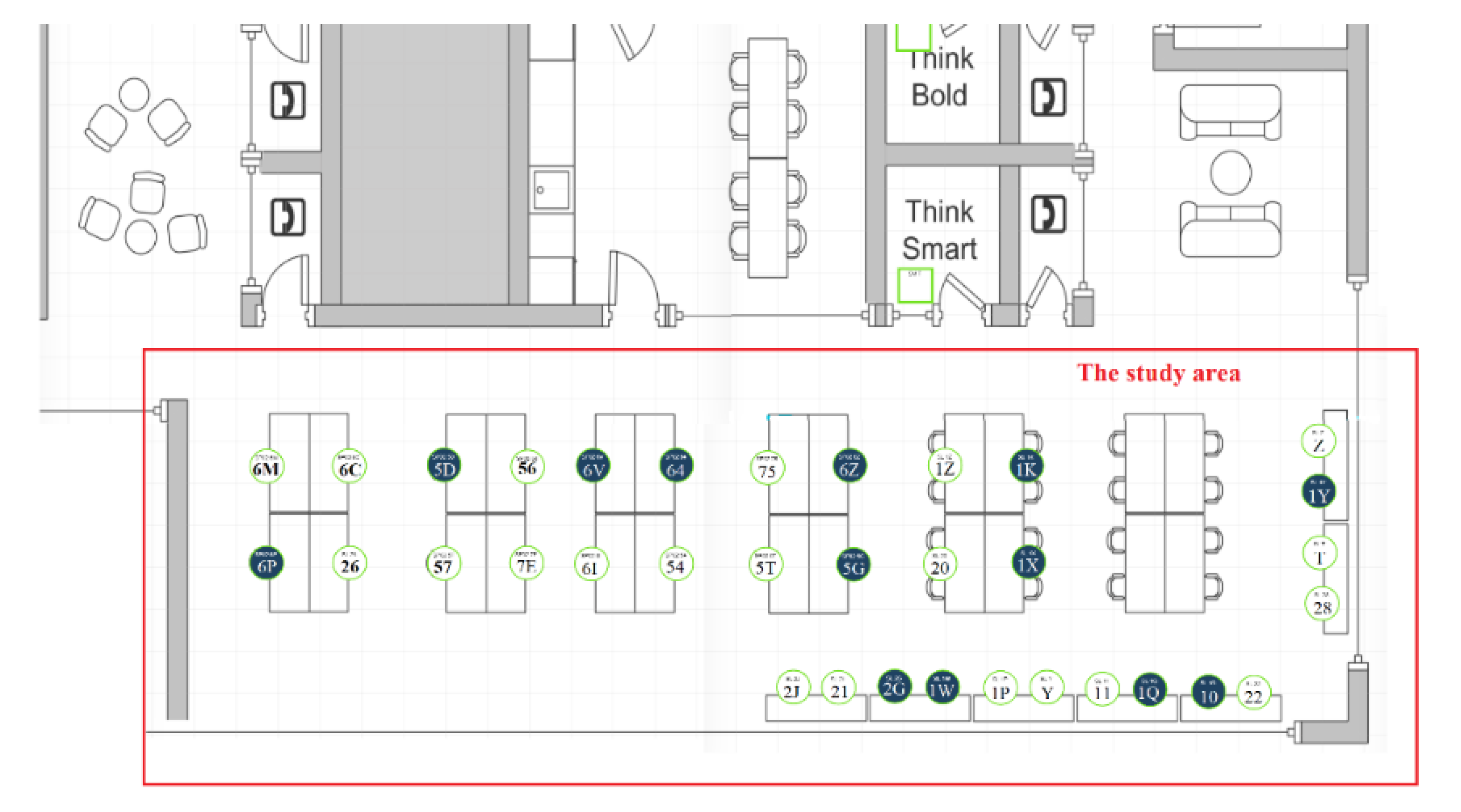
The object of research is an open-space office building in Vilnius. In premises, the PIR motion detectors were installed at each workstation under the table (Figure 2). Workstations (desks) were numbered and the numbers at the desks were assigned to a certain PIR sensor (Figure 3).
Real measurements were performed for the period from 8 September 2019 to 12 December 2019 and there were 32 observed workstations in the area. Therefore, it was possible to accurately determine the exact number of people in the room at any time during working hours, and the variation of their presence during this period. The motion sensors collected data for each workstation separately, so each workstation file was processed separately and placed in a single room occupancy file.
According to the energy performance certificate, the predicted energy consumption for heating was 19.44 kWh/m2/year. However, the actual energy consumption was 67 kWh/m2/year. The performance gap is obvious and makes 3 times more than predicted.
3.2. Mathematical Modelling with Extreme Learning Machine Method
Extreme learning machine (ELM) method has gained increasing attention from various research fields recently [53,54,55,56,57,58]. It has wide application, such as the forecasting of gasoline octane number, for the detection of machine failure error, in medicine and other disciplines. ELM application for occupancy prediction is still not common, even though it is fast and has high accuracy. This method is a simple and efficient single-hidden layer feedforward neural network (SLFNN) [57,58]. The key idea of ELM is to randomly generate the weights between the input layer and the hidden layer, and analytically calculate the output weights by using Moore–Penrose generalized inverse. ELM is formulated as a linear-in-the-parameter model, which boils down to solving a linear system. ELM appears to be suitable in applications, which inquire fast prediction and response capability [57], therefore authors made a hypothesis that advantages of this method would enable to forecast occupancy behaviour in the building.
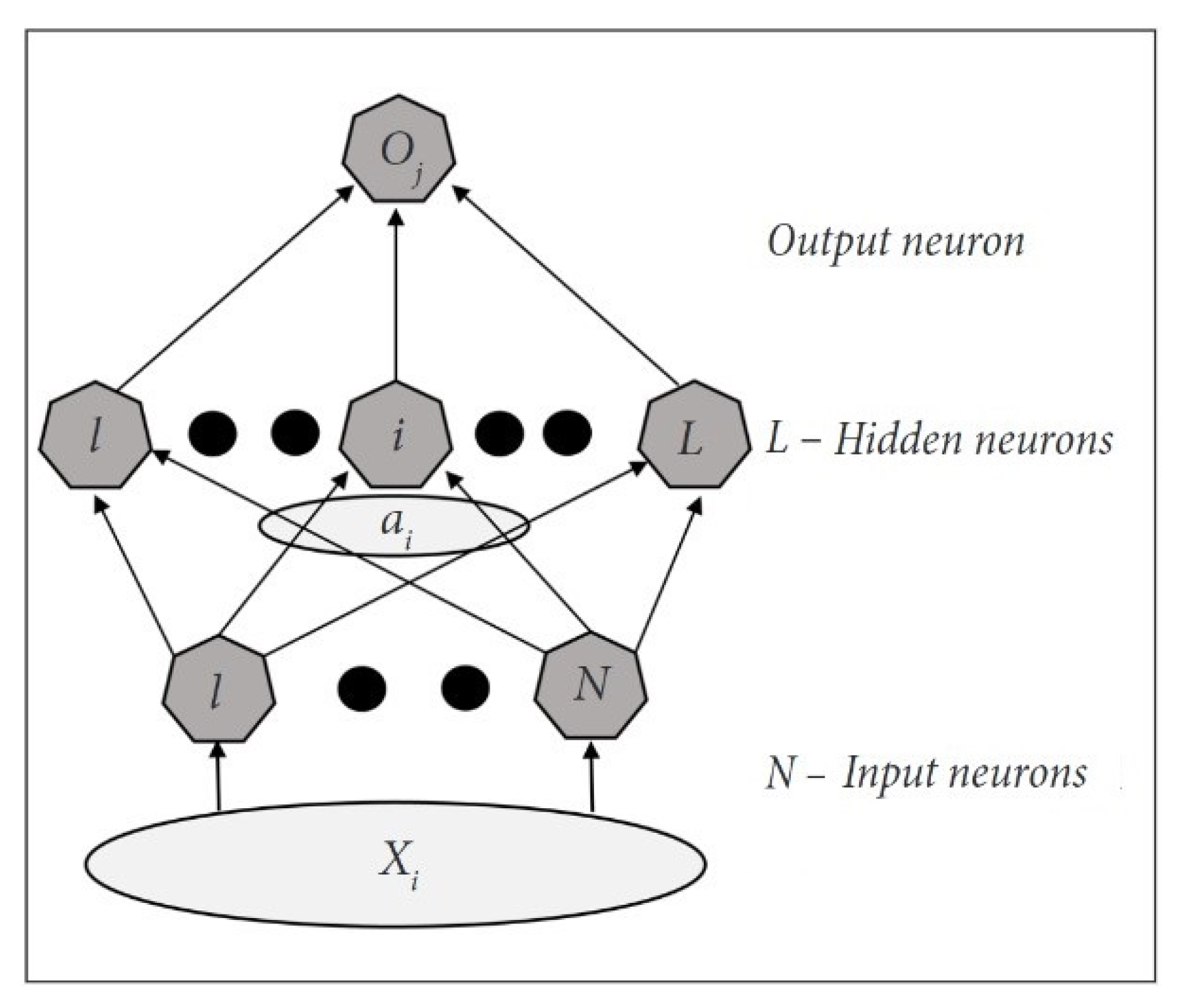
Figure 4 presents an example of a simple single layer feedforward neural network (SLFNN), for N arbitrary distinct samples (xi, ti), where xi = [xi1, xi2, ..., xin]T ∈ Rn, and ti = [ti1, ti2, ..., tim]T∈ Rm is the input and output data sample. The SLFNN with L hidden nodes and activation function gi(x) is modelled mathematically.
Huang et al. [56] proposed a modification of the changes based on the least squares (LS) training course used in the online sequential extreme learning machine (OS-ELM). OS-ELM creates a better summary search and learns very quickly:
where j = 1, ..., N, gi(x)–activation function, which can be different: linear, sigmoidal or tangential; wi = (wi1, wi2, ..., wim)T–weight vector, connecting the ith hidden neurons and the input neurons; βi = (βi1, βi2, ..., βim)T–is the weight vector connecting the ith hidden neuron and the output neurons; bi–threshold of the ith hidden neuron. Inner product of wi and xj is denoted as wi ∙ xj. The output neurons are assumed to be linear.
In a standard SFLNN, a calculation scheme with L hidden nodes and activation function gi(x) can approximate these L samples that , i.e., there exist such βi, wi, bi, that:
The above given N equations can be written as Hβ = T and expressed as matrix:
β = (β1, β2, ..., βL) the so-called Huang [54,55] neural network hidden layer output matrices. The ith column of matrix H, the so-called output of the ith neuron with corresponding input neurons (x1, x2, ..., xL). Activation and transfer functions are always infinitely differentiated and the number of samples is significantly larger than the number of hidden neurons L << N.
ELM consists of the main following steps:
- Random selection of the input weights wi and bi, where i = 1, ..., L;
- Calculation of the hidden layer output matrix H;
- Calculation of the output weights β: β = , where T = [t1, t2, ..., tN]T.
The main properties of the model are as follows:
Minimum training error. The special solution β* = T is one of the least-squares solutions of a general linear system Hβ = T, meaning that the smallest training error can be reached by this special solution:
Although almost all learning algorithms wish to reach the minimum training error, however, most of them cannot reach it because of local minimum or infinite training iterations.
Smallest norm of weights. The special solution β* = T has the smallest norm among all the least-squares solutions of Hβ = T:
Minimum Hβ = T least-squares solutions norm is the only one and equal to β* = T.
Activation function g(x) is infinitely differentiated, as may be sigmoidal functions and the radial basis, sine, cosine, exponential and many other non-regular functions [53], as well as the upper bound of the required number of hidden neurons, which is much more less than the number of distinct training samples, that is L << N.
To get the neural network structure employing evolutionary algorithms, the following components of the neurons network must be defined:
- Inputs number;
- Number of hidden layers and number of neurons;
- Transfer function;
- Outputs number;
The differential evolution (DE) method for minimizing the continuous space functions has been introduced by Storn and Price [53]. DE is a parallel direct and random search method [60]. The initial vector population was chosen randomly and should cover the entire parameter space. The population was represented by population size—NP, number of decision variables—D, dimension parameter—hl (h = 1, 2, ..., NP and l = 1, 2, ..., D).
Mutation. By randomly selecting and subtracting two different individual vectors, the difference vectors are generated. The difference vectors are weighed and added to the third randomly selected individual vectors and the variation vectors are generated. For each individual, xht a mutation is performed using Equation (7):
with random indexes r1, r2, r3 ∈ {1, 2, ..., NP}, integer, mutually different and K > 0. K is a real and constant factor, which controls the amplification of the differential variation.
Cross-over. The purpose of this action is to generate test vectors mixing a variation vector with the target vector (to increase the diversity of the perturbed parameter vectors). The cross-operation of xht with a variant individual vht+1 to generate experimental individual (test vector) uht+1 is performed using Equation (8):
In Equation (8) rand (l) is the lth evaluation of a uniform random number generator with the outcome ∈ [0,1]; CR is a cross-over constant ∈ [0,1] and rnbr (h) is a randomly chosen index ∈ {1, 2, ..., D}.
Selection. If the test vector uht+1 yields a lower cost function value than the target vector, the test vector replaces the target vector in the next generation. Each population vector has to serve once as the target vector so that the NP competitions take place in one generation. The minimization problem is solved:
where J is a fitness function.
4. Results
4.1. Results of the Experimental Research
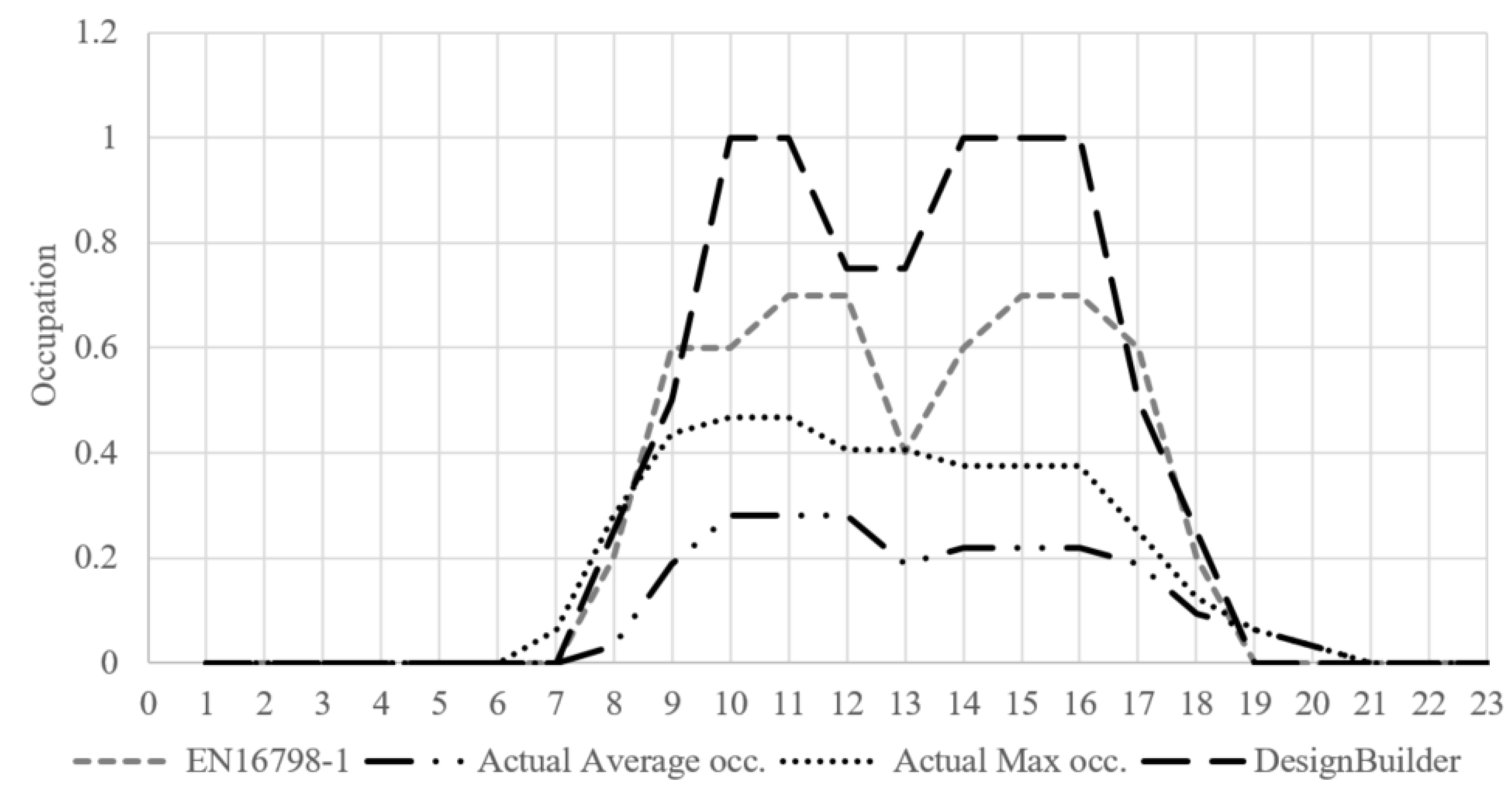
Figure 6 presents a comparison of the occupancy profiles used in simulations. Actual determined occupancy is the arithmetic mean of the specific hour over the measured period and the maximum past occupation.
Figure 6 shows that actual occupancy is much lower than the default assumptions representative for a typical occupancy pattern. This situation can be explained by the fact that typical occupancy profiles do not take into account the peculiarities of activities in considered building types. The premises of the open-space office building where the experimental research was conducted are occupied by the company that mainly focuses on renewable energy technologies. The company develops alternative energy projects across Europe, including biogas and solar power plants. The experienced team consists mainly of engineers, who often go to construction sites and numerous existing buildings to install or maintain equipment. The work, which involves a lot of movement from the office, is quite common in construction and engineering companies, but high mobility is not considered in typical occupancy patterns. Therefore, in the future, it is necessary to monitor more open-space offices and to identify new or revise existing occupancy assumptions.
Figure 7 shows the actual hourly average occupation for each working day. The graph shows that all working days are similar. The actual occupancy was significantly lower than the one given in normative document EN 16798-1 or DesignBuilder as default schedule. The actual occupancy trend is similar to the other cases—showing peaks at similar periods of the day, also showing that during lunchtime occupancy decreases, but fluctuations during the day for the actual case are low compared to the other cases. This can be explained by very low actual occupancy and the high mobility of the occupants, as they do not have their workstations, they are coming to the office just to perform certain tasks and then leaving again. This is also an indication for an employer, that such style of mobile work does not need so much space to rent as this is a waste of resources—energy and financial as well.
The experimentally defined occupancy schedules in an open-space office have shown that actual occupancy is less for about 3.5 times compared to the default DesignBuilder’s schedules and 2.7 times less compared to the ones given in EN 16798-1.
It is obvious from the occupancy and indoor parameter measurements that lower occupation cannot be the main cause of the performance gap in the analysed building. Lower occupation in this building may cause just lower heat gains in winter and thus higher energy demand for heating. Within the measured period, it was found that the inside temperatures in winter were maintained much higher (average 23 °C), compared to the ones used in the prediction phase according to the national energy performance certification methodology (20 °C). Other possible reasons causing the performance gap were not analysed as they were out of scope of this study.
4.2. Results of the Forecast Applying Extreme Learning Machine Method
Experiments enabled to define passive occupancy behaviour, e.g., average actual occupancy profiles. In addition, indoor parameters—air temperature, relative humidity, CO2 concentration, air velocity and outdoor parameters—air temperature, relative humidity and solar radiation were measured. Measurements were performed for the period from the 8th of August to the 21st of December 2019, but reliable data are considered just for the period from the 26th of August to the 21st of October.
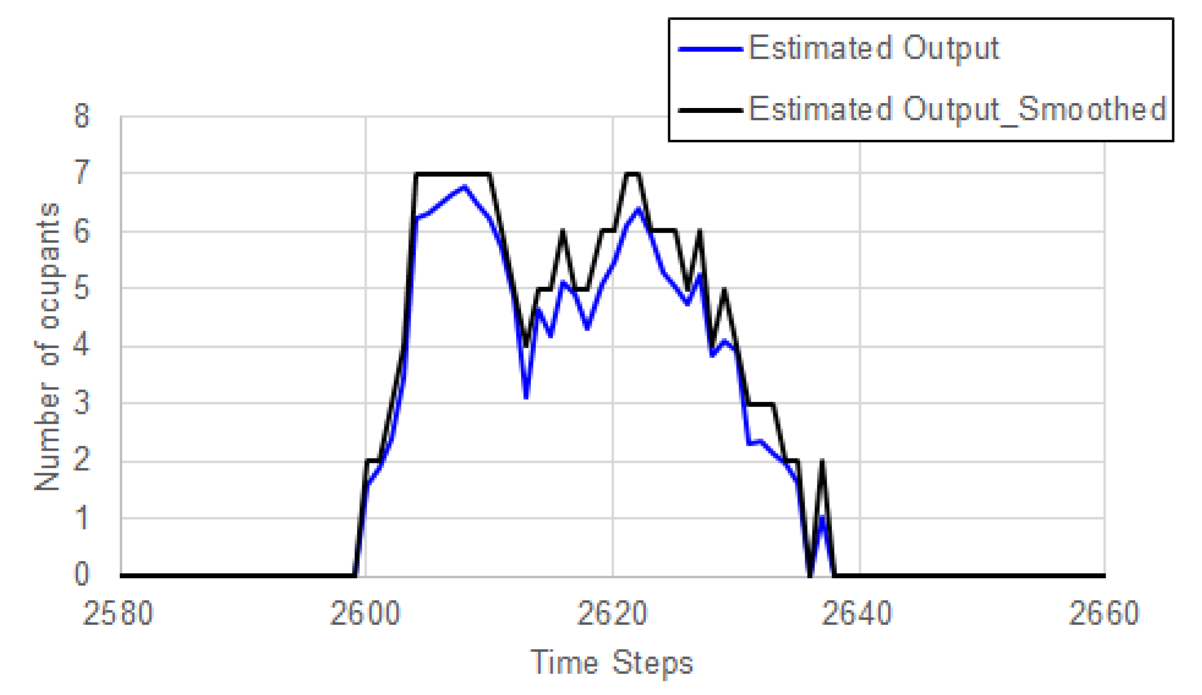
Before forming the neural network model, data smoothing was performed, and an example of one-day smother data is presented in Figure 8. Smoothing is required for non-working hours as there might be discrepancies because HVAC system control is turned off at the end of the working day and such parameters as indoor temperature, CO2 concentration, and relative humidity are reacting to that fact very slowly.
When the neural network model was formed, the learning algorithm was programmed with MATLAB with the sample size of the unfiltered data—16,279 points. The time step between the measured values was 5 min. Out of the total data, 60% were used as a training set, 10%—as a testing set and 30% for the validation of the predicted results.
Having the goals to define the significance of different input data sets and to assess the applicability of the OSELM with a DE method in occupancy passive behaviour forecasting, the simulation with MATLAB learning algorithms was performed in III stages:
Stage I. Based on measured input variables (xi), occupancy profiles are modelled for different input data combinations:
- (1)
- Indoor Parameters:
- Carbon dioxide (CO2) concertation, ppm;
- Indoor air temperature (Tin), °C;
- Relative air humidity (RHin), %;
- (2)
- Outdoor Parameters:
- Solar radiation (Gout), W/m2;
- Air temperature (Tout), °C;
- Relative air humidity (RHout), %;
- (3)
- Both Indoor and Outdoor Parameters.
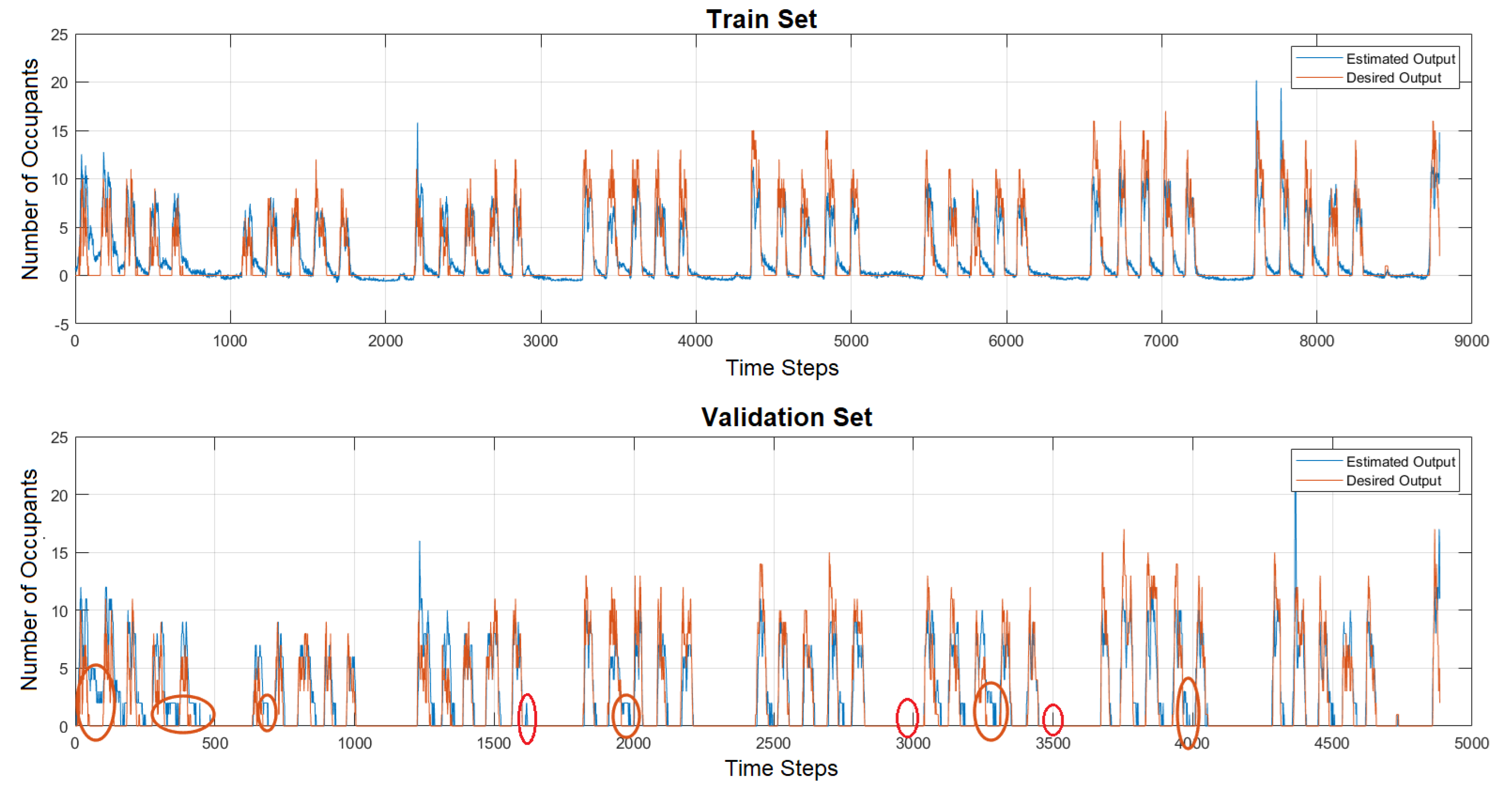
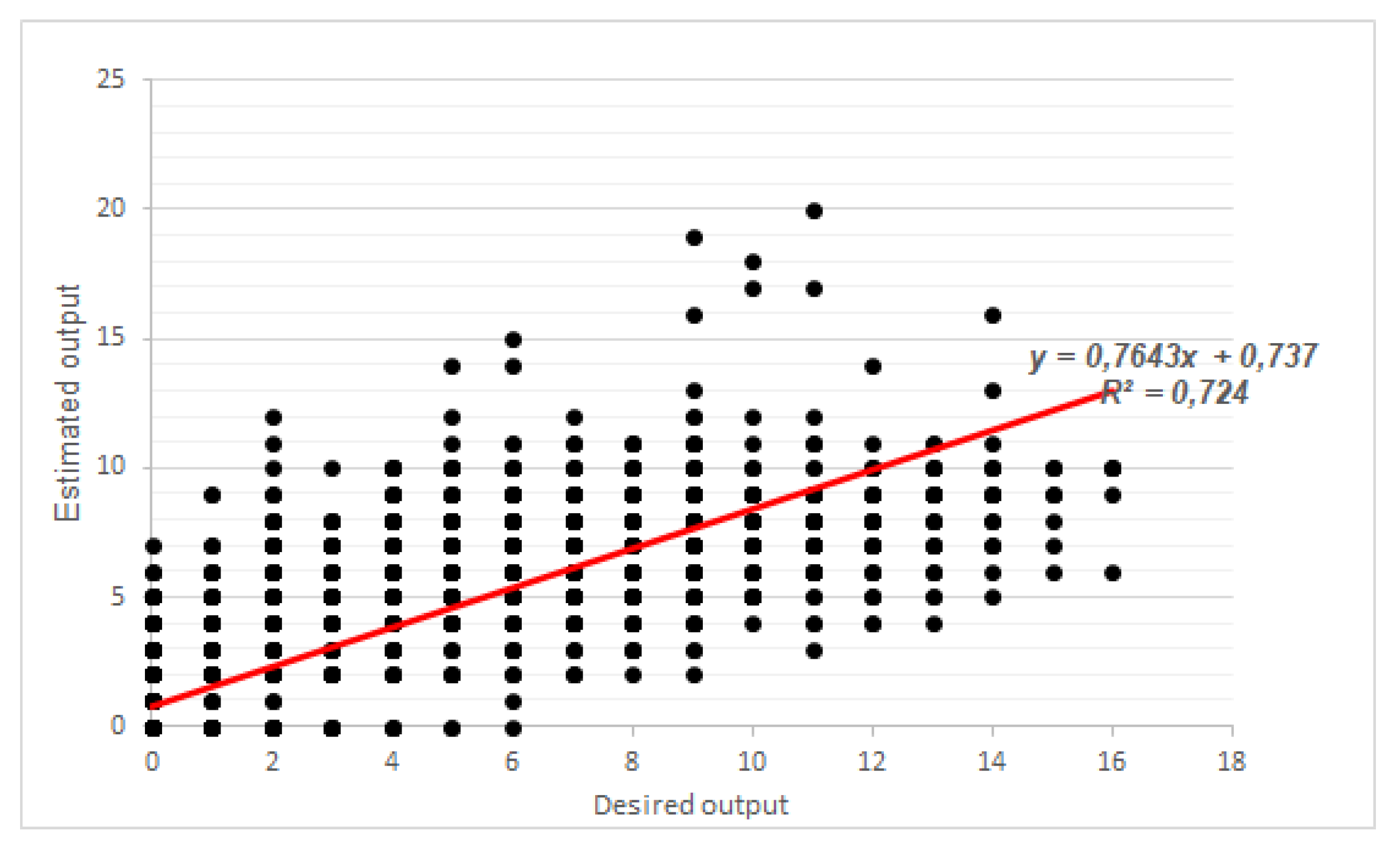
After modelling was performed with indoor and outdoor parameters (Figure 9), it was noticed that there are some forecasting errors during unoccupied hours—during the night and weekends (see red circles on Figure 9). Calculated correlation coefficient R2 for this data set is 0.72, its graphical representation is shown in Figure 10.
The accuracy of results is considered as good compared to the results of other researchers, who analysed occupancy with high fluctuations, using the same variables as in this paper, but different prediction methods. Ai et al. [34] used the hidden Markov model (HMM) and autoregressive hidden Markov model (ARHMM) for occupancy prediction, and the models showed an accuracy of 25% for HMM and 80.1% for ARHMM, respectively. Dong et al. [30] used the HHM, Support Vector Machines (SVM) and Artificial Neural Network (ANN) methods and declared an accuracy of forecasting results varying from 58% to 75%.
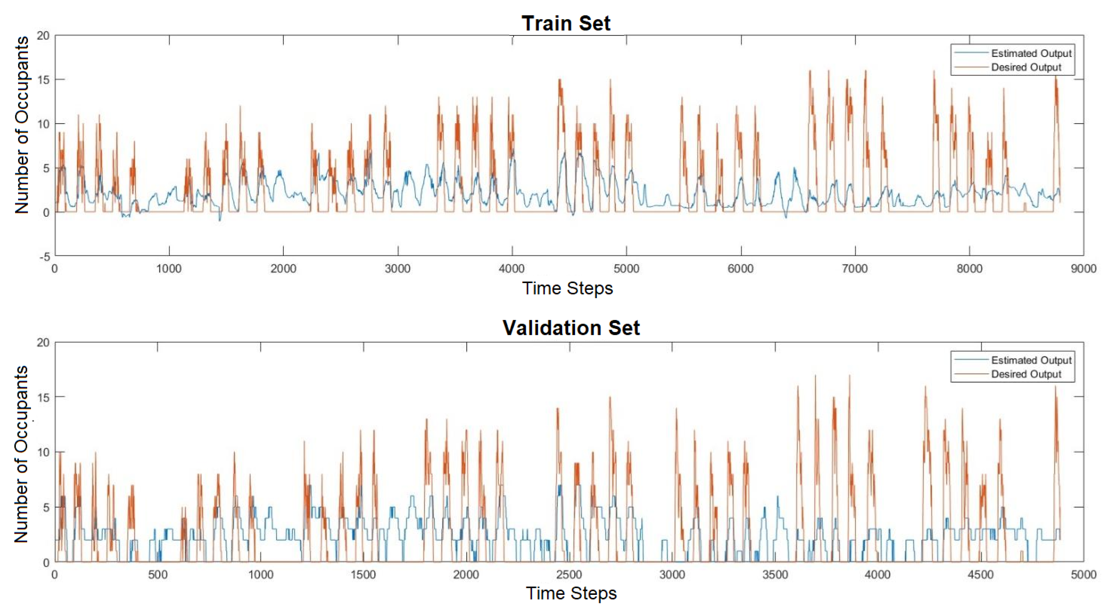
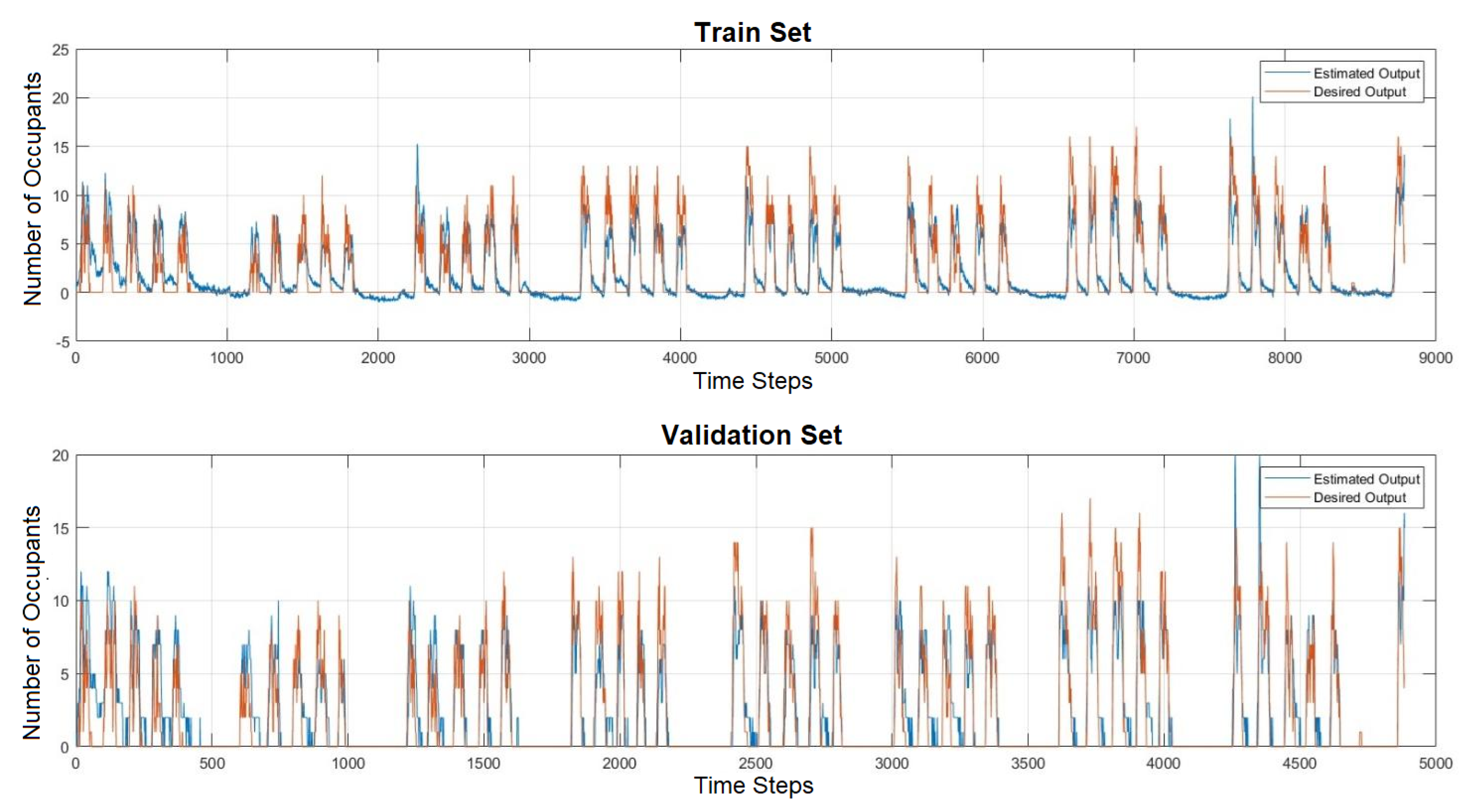
Separate modelling was performed to define which data set (indoor or outdoor) had the highest impact on the accuracy of occupancy prediction. The calculation results are depicted in Figure 11 and Figure 12. Modelling results have shown that the correlation coefficient R2 for the modelling based on the data set (xi) of indoor parameters is 0.72 and for the modelling based on the outdoor data set is 0.15. Thus, it is obvious that the forecasting of occupancy behaviours based only on an outdoor data set is inappropriate, as the correlation of the occupancy is very low.
Stage II. ELM modelling for separate weeks with an indoor data set:
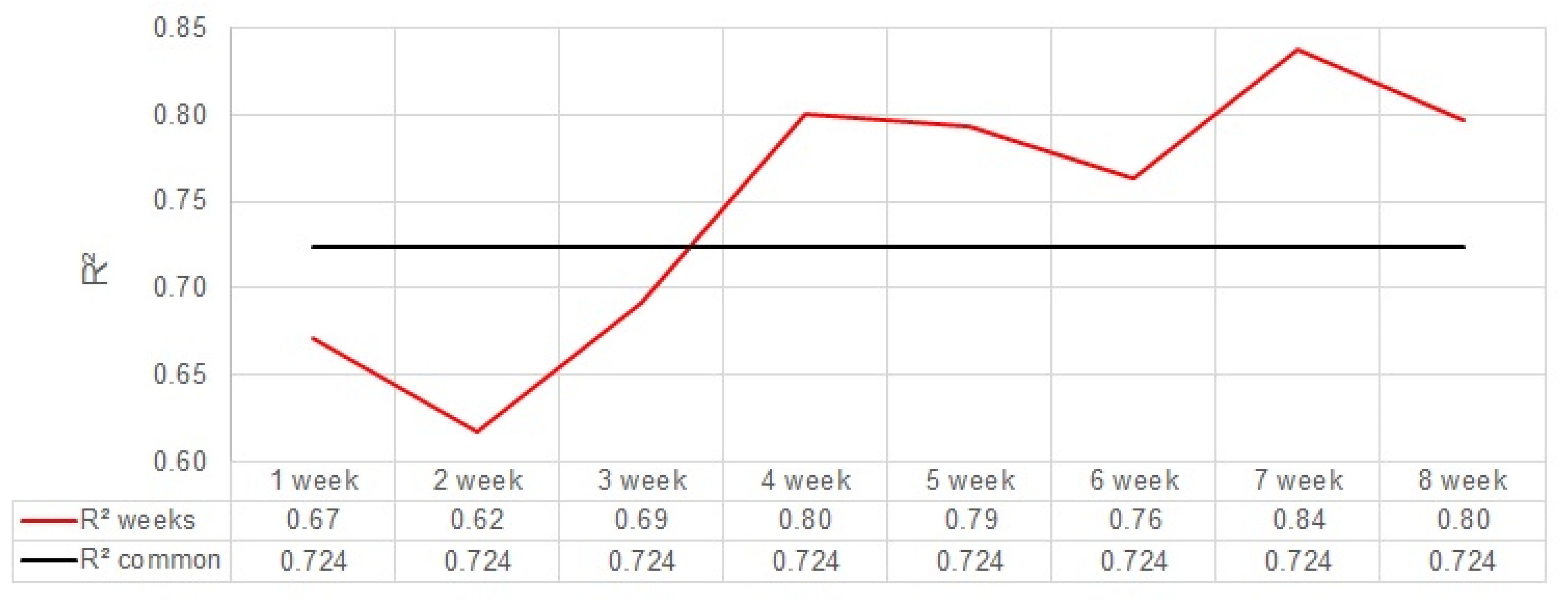
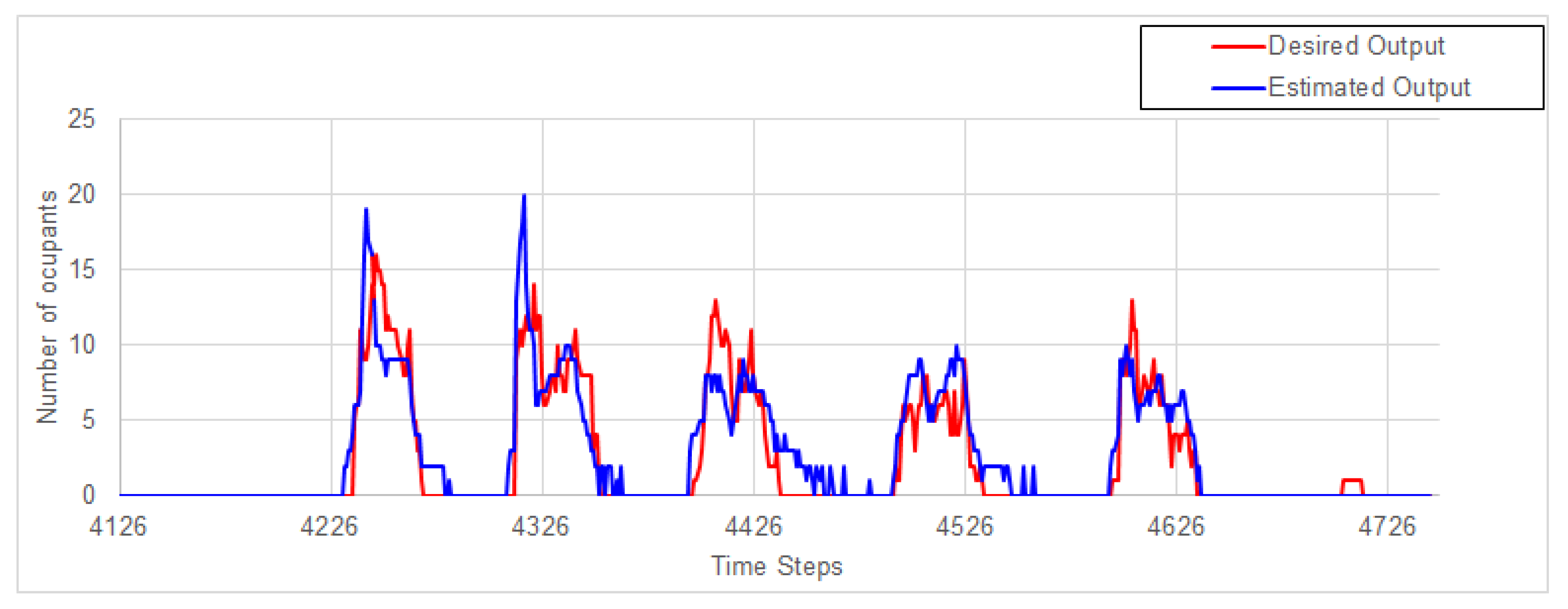
Since the modelling based on the indoor parameters’ (Tin, RHin, CO2) data set showed the best correlations, it was further explored in more detail by modelling shorter periods—weeks. Modelling with indoor parameters, when unoccupied hours are not eliminated, resulted in the correlations R2 varying from 0.62 to 0.84 (Figure 13). The first three simulated weeks showed worse results and starting from the fourth modelled week, the accuracy increased (Figure 14), as the input data set size increases, thus emphasizing the importance of the size of the data set on prediction accuracy.
From the above-shown results, it can be concluded that the application of DE-OSELM for occupancy prediction shows good results and that the 4 weeks‘ measured period might be considered already as a reasonable measurement period for the reliable prediction of the building’s occupancy.
Stage III. To explore which of the indoor parameters gives the best prediction accuracy:
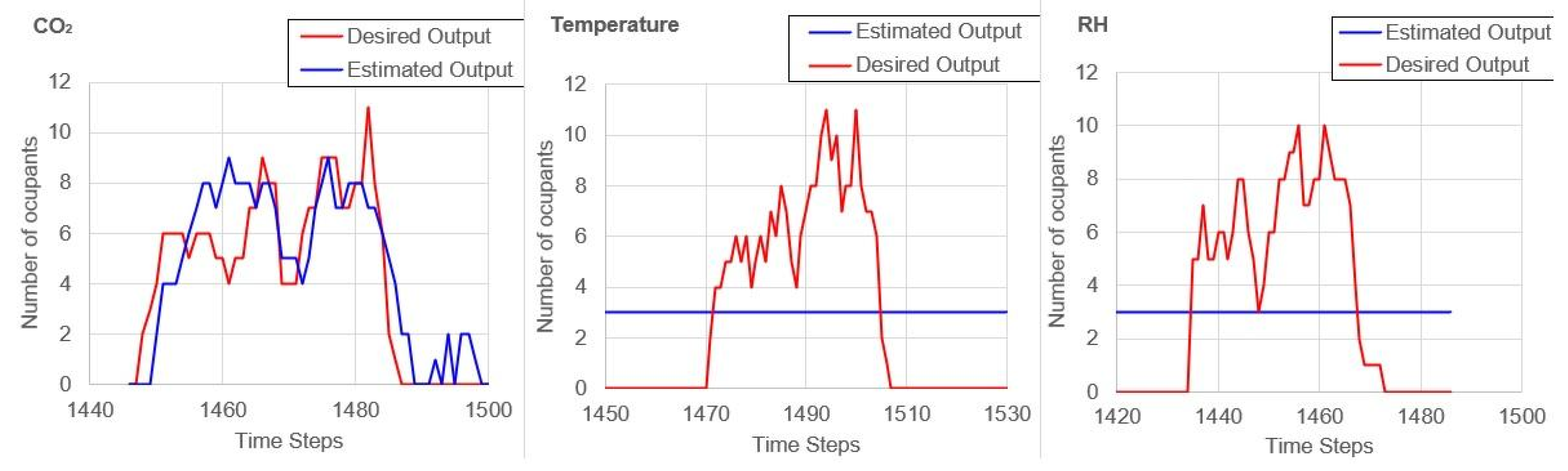
Due to weak correlations, the outdoor parameters were not analysed further. The indoor parameters, modelled as separate variables (xi), sought to define which one was the most suitable for occupancy prediction. Modelling was performed for one selected day of the measured period. The results given in Figure 15 illustrate that air temperature and relative humidity make almost no influence on occupancy. Meanwhile, the forecasting according to CO2 gives a very good correlation coefficient R2 equal to 0.84 for one day and 0.71 for all the analysed period. The correlation coefficient R2 increases just by 0.01 if we analyse together the data of indoor temperature and relative humidity.
From the presented results, the conclusion arose that occupancy prediction according to the outdoor data set is inappropriate, as it has no influence on occupancy. The most appropriate is forecasting occupancy according to the indoor parameters, where CO2 is the main parameter resulting in the best correlation coefficient R2 values. Relative air humidity and air temperature increase the forecasting accuracy, which is insignificant but still positive. Therefore, to predict future occupancy patterns, the historical indoor CO2 data can be considered as a sufficient parameter.
Analysis of the OSELM with DE model prediction accuracy for separate weeks showed that the accuracy increases with the size of the data set, e.g., the data gained from 4 weeks’ measurements can be considered as sufficient for the forecasting, as R2 is 0.8 already for the 4th week, for the later weeks, it increases to a maximum of 0.84.
Such forecasting may be used to adapt indoor parameters in the space before the occupants arrive and to adjust operation modes of the HVAC equipment, especially ventilation airflow rates, based on forecasted occupancy. The DE-OSELM model is proved as suitable for adaptive buildings because of its high prediction accuracy and fast prediction process.
5. Discussion and Conclusions
The experimentally defined occupancy schedules in an open-space office have shown that actual occupancy is less for about 3.5 times compared to the default DesignBuilder’s schedules and 2.7 times less compared to the ones given in EN 16798-1. This shows that the DesignBuilder- and EN16798- given occupants’ presence profiles are suitable to predict just typical open-space offices, e.g., banks, or call centres, where the occupants’ working hours are strictly fixed. For the offices with flexible working hours and high mobility exists a demand to predict the occupants’ presence using historical data and a demand for fast and reliable mathematical forecasting models.
Occupancy behaviour prediction is analysed by many researchers by applying different models and based on differently measured data. Hence, the results have limited application and limited accuracies. The accuracy of prediction in the applied DE-OSELM model is increased using separately measured indoor and outdoor data sets (variables). From a learning efficiency point of view, the DE-OSELM model has three advantages: the least human intervention, high learning accuracy and a fast learning speed. The reliability of the obtained results strongly depends on the size of the data set, as an insufficient number of data causes a low prediction accuracy. In the presented study, the sample data size is 16,279 points and is considered as sufficient compared to the number used by similar studies. In addition, it is very important to choose proper input variables (xi), as they strongly influence the prediction accuracy.
Input variables (xi) used in the study were grouped into indoor and outdoor parameters. It was found that the prediction using an unfiltered data set of indoor and outdoor parameters resulted in the highest accuracy as the R2 correlation coefficient was 0.72, meanwhile, when only the outdoor data set was used, R2 equalled just 0.15.
Indoor data influence on the prediction accuracy was also explored separately for each parameter (input variable) and it was found that temperature and humidity almost have no influence on occupancy prediction, as their fluctuations are low. The CO2 correlation with occupancy was the highest—R2 equalled to 0.84 for one day and 0.71 for all the analysed period, which was considered as very high accuracy. To predict the future occupancy patterns, the historical indoor CO2 data can be considered as the sufficient parameter. It was also confirmed by Jiang et al. [12].
The analysis of the prediction accuracy by separate weeks have shown that a 4 week measurement period might be considered already as reasonable for the reliable prediction of the building’s occupancy.
The limitations of the experimental data are related to the measured period—the influence of the season of the year, and parameters such as different clothing, shorter winter days, and the possible absence because of illnesses were not taken into account. Longer data collection periods will be analysed in the future as it will result in bigger data sets and this will also possibly influence the higher accuracy of the results obtained using the proposed prediction model.
Although the accuracy of the prediction obtained in the present case can be considered as very high, additional input variables related to the social aspects of occupants’ behaviour need to be found and included in the future in order to improve the prediction accuracy. For this purpose, additional surveys of occupants are needed. The companies’ type of activities and the peculiarities of the personnel management system are required. Such a “force majeure” as COVID-19 has significantly changed the arrangements of office work, as many people started working remotely, and this may strongly influence the change in the future occupation of the offices, even after the pandemic period. The required office floor area per occupant may decrease, and HVAC system operation will have to be adapted. Thus, to avoid an increase in performance gap, the demand for occupancy prediction models has the potential to increase.
Author Contributions
Conceptualization, V.M. and J.B.; methodology, J.B. and A.I.; validation, J.B., A.I. and V.M.; formal analysis, V.M., T.V.; investigation, J.B.; resources, T.V.; data curation, V.M.; writing—original draft preparation, V.M., J.B.; writing—review and editing, T.V.; visualization, J.B. and V.M.; supervision, V.M. All authors have read and agreed to the published version of the manuscript.
Funding
This research was funded by a grant (No. S-MIP-20-62) from the Research Council of Lithuania.
Acknowledgments
The authors would like to express their sincere gratitude to Jonas Bielskus for his technical support during the performance of measurements.
Conflicts of Interest
The authors declare no conflict of interest.
References
- Huovila, P.; Ala-Juusela, M.; Melchert, L.; Pouffary, S.; Cheng, C.C.; Ürge-Vorsatz, D.; Koeppel, S.; Svenningsen, N.; Graham, P. Buildings and Climate Change: Summary for Decision Makers; Yamamoto, J., Graham, P., Eds.; United Nations Environment Programme (UNEP DTIE): Paris, France, 2009; p. 60. [Google Scholar]
- Martinaitis, V.; Zavadskas, E.K.; Motuziene, V.; Vilutiene, T. Importance of occupancy information when simulating energy demand of energy efficient house: A case study. Energy Build. 2015, 101, 64–75. [Google Scholar] [CrossRef]
- Paone, A.; Bacher, J.P. The impact of building occupant behavior on energy efficiency and methods to influence it: A review of the state of the art. Energies 2018, 11, 953. [Google Scholar] [CrossRef] [Green Version]
- RIBA CIBSE Platform CarbonBuzz. Available online: https://www.carbonbuzz.org/index.jsp (accessed on 12 June 2020).
- Delzendeh, E.; Wu, S.; Lee, A.; Zhou, Y. The impact of occupants’ behaviours on building energy analysis: A research review. Renew. Sustain. Energy Rev. 2017, 80, 1061–1071. [Google Scholar] [CrossRef]
- Peper, S.; Feist, W. Monitoring und Bilanzrechnung: Ganz ohne Performance GAP. In Proceedings of the CESBP Central European Symposium on Building Physics and BauSIM 2016, Fraunhofer IRB Verlag, Dresden, Germany, 14–16 September 2016; pp. 267–275. [Google Scholar]
- Hong, T.Z.; Taylor-Lange, S.C.; D’Oca, S.; Yan, D.; Corgnati, S.P. Advances in research and applications of energy-related occupant behavior in buildings. Energy Build. 2016, 116, 694–702. [Google Scholar] [CrossRef] [Green Version]
- Schweiker, M.; Ampatzi, E.; Andargie, M.S.; Andersen, R.K.; Azar, E.; Barthelmes, V.M.; Berger, C.; Bourikas, L.; Carlucci, S.; Chinazzo, G.; et al. Review of multi-domain approaches to indoor environmental perception and behaviour. Build. Environ. 2020, 176, 25. [Google Scholar] [CrossRef]
- Zhang, Y.; Bai, X.M.; Mills, F.P.; Pezzey, J.C.V. Rethinking the role of occupant behavior in building energy performance: A review. Energy Build. 2018, 172, 279–294. [Google Scholar] [CrossRef]
- Balvedi, B.F.; Ghisi, E.; Lamberts, R. A review of occupant behaviour in residential buildings. Energy Build. 2018, 174, 495–505. [Google Scholar] [CrossRef]
- Masood, M.K.; Soh, Y.C.; Chang, V.W.C. Real-time occupancy estimation using environmental parameters. In Proceedings of the International Joint Conference on Neural Networks (IJCNN), Killarney, Ireland, 12–17 July 2015; IEEE: Killarney, Ireland, 2015. [Google Scholar]
- Jiang, C.Y.; Masood, M.K.; Soh, Y.C.; Li, H. Indoor occupancy estimation from carbon dioxide concentration. Energy Build. 2016, 131, 132–141. [Google Scholar] [CrossRef] [Green Version]
- Chen, Z.H.; Masood, M.K.; Soh, Y.C. A fusion framework for occupancy estimation in office buildings based on environmental sensor data. Energy Build. 2016, 133, 790–798. [Google Scholar] [CrossRef]
- Liu, T.C.; Li, Y.; Bai, Z.; De, J.; Le, C.V.; Lin, Z.P.; Lin, S.H.; Huang, G.B.; Cui, D.S. Two-stage structured learning approach for stable occupancy detection. In Proceedings of the International Joint Conference on Neural Networks (IJCNN), Vancouver, Canada, 24–29 July 2016; IEEE: Vancouver, Canada, 2016; pp. 2306–2312. [Google Scholar]
- Masood, M.K.; Jiang, C.Y.; Soh, Y.C. A novel feature selection framework with Hybrid Feature-Scaled Extreme Learning Machine (HFS-ELM) for indoor occupancy estimation. Energy Build. 2018, 158, 1139–1151. [Google Scholar] [CrossRef]
- Chen, Z.H.; Jiang, C.Y.; Xie, L.H. A novel ensemble elm for human activity recognition using smartphone sensors. Ieee Trans. Ind. Inform. 2019, 15, 2691–2699. [Google Scholar] [CrossRef]
- Wei, Y.X.; Xia, L.; Pan, S.; Wu, J.S.; Zhang, X.X.; Han, M.J.; Zhang, W.Y.; Xie, J.C.; Li, Q.P. Prediction of occupancy level and energy consumption in office building using blind system identification and neural networks. Appl. Energy 2019, 240, 276–294. [Google Scholar] [CrossRef]
- Jiang, C.Y.; Chen, Z.H.; Su, R.; Masood, M.K.; Soh, Y.C. Bayesian filtering for building occupancy estimation from carbon dioxide concentration. Energy Build. 2020, 206, 109566. [Google Scholar] [CrossRef]
- Sun, Y.; Haghighat, F.; Fung, B.C.M. A review of the -state-of-the-art in data -driven approaches for building energy prediction. Energy Build. 2020, 221, 110022. [Google Scholar] [CrossRef]
- Schaumann, D.; Pilosof, N.P.; Sopher, H.; Yahav, J.; Kalay, Y.E. Simulating multi-agent narratives for pre-occupancy evaluation of architectural designs. Autom. Constr. 2019, 106, 19. [Google Scholar] [CrossRef]
- Agyeman, K.A.; Kim, G.; Jo, H.; Park, S.; Han, S. An ensemble stochastic forecasting framework for variable distributed demand loads. Energies 2020, 13, 20. [Google Scholar] [CrossRef]
- Li, Z.H.; Friedrich, D.; Harrison, G.P. Demand forecasting for a mixed-use building using agent-schedule information with a data-driven model. Energies 2020, 13, 20. [Google Scholar] [CrossRef] [Green Version]
- Gucyeter, B. Evaluating diverse patterns of occupant behavior regarding control-based activities in energy performance simulation. Front. Archit. Res. 2018, 7, 167–179. [Google Scholar] [CrossRef]
- Yamaguchi, Y.; Shimoda, Y.; Mizuno, M. Development of district energy system simulation model based on detailed energy demand. In Proceedings of the Eighth International IBPSA Conference, Eindhoven, The Netherlands, 11–14 August 2003; Volume 8, pp. 1443–1450. [Google Scholar]
- Page, J.; Robinson, D.; Morel, N.; Scartezzini, J.L. A generalised stochastic model for the simulation of occupant presence. Energy Build. 2008, 40, 83–98. [Google Scholar] [CrossRef]
- Wang, C.; Yan, D.; Jiang, Y. A novel approach for building occupancy simulation. Build. Simul. 2011, 4, 149–167. [Google Scholar] [CrossRef]
- Chen, Z.H.; Xu, J.M.; Soh, Y.C. Modeling regular occupancy in commercial buildings using stochastic models. Energy Build. 2015, 103, 216–223. [Google Scholar] [CrossRef]
- Chen, Z.; Soh, Y.C. Modeling building occupancy using a novel inhomogeneous Markov chain approach—IEEE Conference Publication. In Proceedings of the IEEE International Conference on Automation Science and Engineering (CASE), Taipei, Taiwan, 18–22 August 2014. [Google Scholar]
- Lam, K.P.; Höynck, M.; Dong, B.; Andrews, B.; Chiou, Y.S.; Zhang, R.; Benitez, D.; Choi, J. Occupancy detection through an extensive environmental sensor network in an open-plan office building. In Proceedings of the Eleventh International IBPSA Conference, Glasgow, UK, 27–30 July 2009. [Google Scholar]
- Dong, B.; Andrews, B.; Lam, K.P.; Hoynck, M.; Zhang, R.; Chiou, Y.S.; Benitez, D. An information technology enabled sustainability test-bed (ITEST) for occupancy detection through an environmental sensing network. Energy Build. 2010, 42, 1038–1046. [Google Scholar] [CrossRef]
- Dong, B.; Lam, K.P. Building energy and comfort management through occupant behaviour pattern detection based on a large-scale environmental sensor network. J. Build. Perform. Simul. 2011, 4, 359–369. [Google Scholar] [CrossRef]
- Han, Z.Y.; Gao, R.X.; Fan, Z.Y. Occupancy and indoor environment quality sensing for smart buildings. In Proceedings of the 29th Annual IEEE International Instrumentation and Measurement Technology Conference (I2MTC), Graz, Austria, 13–16 May 2012; IEEE: Graz, Austria; pp. 882–887. [Google Scholar]
- Sandels, C.; Widen, J.; Nordstrom, L. Simulating occupancy in office buildings with non-homogeneous markov chains for demand response analysis. In Proceedings of the 2015 IEEE Power & Energy Society General Meeting, Denver, CO, USA, 26–30 July 2015; pp. 1–5. [Google Scholar] [CrossRef] [Green Version]
- Ai, B.; Fan, Z.; Gao, R.X. Occupancy estimation for smart buildings by an auto-regressive hidden Markov model—IEEE Conference Publication. In Proceedings of the IEEE Conference—American Control Conference (ACC), Portland, OR, USA, 4–6 June 2014; pp. 2234–2239. [Google Scholar]
- Wang, Z.X.; Ding, Y. An occupant-based energy consumption prediction model for office equipment. Energy Build. 2015, 109, 12–22. [Google Scholar] [CrossRef]
- Yang, Z.; Becerik-Gerber, B. Modeling personalized occupancy profiles for representing long term patterns by using ambient context. Build. Environ. 2014, 78, 23–35. [Google Scholar] [CrossRef]
- Milenkovic, M.; Amft, O. Recognizing energy-related activities using sensors commonly installed in office buildings. Procedia Comput. Sci. 2013, 19, 669–677. [Google Scholar] [CrossRef] [Green Version]
- Dobbs, J.R.; Hencey, B.M. Model predictive HVAC control with online occupancy model. Energy Build. 2014, 82, 675–684. [Google Scholar] [CrossRef] [Green Version]
- Dobbs, J.R.; Hencey, B.M. Predictive HVAC control using a Markov occupancy model—IEEE Conference Publication. In Proceedings of the IEEE Conference—American Control Conference (ACC), Portland, OR, USA, 4–6 June 2014. [Google Scholar]
- Virote, J.; Neves-Silva, R. Stochastic models for building energy prediction based on occupant behavior assessment. Energy Build. 2012, 53, 183–193. [Google Scholar] [CrossRef]
- Jain, S.; Madamopoulos, N. Ahorrar: Indoor Occupancy Counting to Enable Smart Energy Efficient Office Buildings—IEEE Conference Publication. In Proceedings of the 2016 IEEE International Conferences on Big Data and Cloud Computing (BDCloud), Social Computing and Networking (SocialCom), Sustainable Computing and Communications (SustainCom) (BDCloud-SocialCom-SustainCom), Atlanta, GA, USA, 8–10 October 2016; pp. 469–476. [Google Scholar]
- Wang, W.; Chen, J.Y.; Song, X.Y. Modeling and predicting occupancy profile in office space with a Wi-Fi probe-based Dynamic Markov Time-Window Inference approach. Build. Environ. 2017, 124, 130–142. [Google Scholar] [CrossRef]
- Salimi, S.; Liu, Z.; Hammad, A. Occupancy prediction model for open-plan offices using real-time location system and inhomogeneous Markov chain. Build. Environ. 2019, 152, 1–16. [Google Scholar] [CrossRef]
- Frei, M.; Deb, C.; Stadler, R.; Nagy, Z.; Schlueter, A. Wireless sensor network for estimating building performance. Autom. Constr. 2020, 111, 17. [Google Scholar] [CrossRef]
- Vanus, J.; Gorjani, O.M.; Bilik, P. Novel proposal for prediction of CO2 course and occupancy recognition in Intelligent Buildings within IoT. Energies 2019, 12, 4541. [Google Scholar] [CrossRef] [Green Version]
- Lee, X.F.; Yang, Y.Y.; Li, R.L.; Nielsen, P.S. A stochastic model for residential user activity simulation. Energies 2019, 12, 3326. [Google Scholar] [CrossRef] [Green Version]
- Jia, M.; Srinivasan, R. building performance evaluation using coupled simulation of energyplus (TM) and an occupant behavior model. Sustainability 2020, 12, 4086. [Google Scholar] [CrossRef]
- Kim, S.; Jung, S.; Baek, S.M. A model for predicting energy usage pattern types with energy consumption information according to the behaviors of single-person households in South Korea. Sustainability 2019, 11, 245. [Google Scholar] [CrossRef] [Green Version]
- Lee, S.; Jung, S.; Lee, J. Prediction model based on an artificial neural network for user-based building energy consumption in South Korea. Energies 2019, 12, 608. [Google Scholar] [CrossRef] [Green Version]
- Chokwitthaya, C.; Zhu, Y.M.; Dibiano, R.; Mukhopadhyay, S. Combining context-aware design-specific data and building performance models to improve building performance predictions during design. Autom. Constr. 2019, 107, 13. [Google Scholar] [CrossRef]
- Diraco, G.; Leone, A.; Siciliano, P. People occupancy detection and profiling with 3D depth sensors for building energy management. Energy Build. 2015, 92, 246–266. [Google Scholar] [CrossRef]
- Pedersen, T.H.; Nielsen, K.U.; Petersen, S. Method for room occupancy detection based on trajectory of indoor climate sensor data. Build. Environ. 2017, 115, 147–156. [Google Scholar] [CrossRef]
- Storn, R.; Price, K. Differential Evolution—A Simple and Efficient Adaptive Scheme for Global Optimization over Continuous Spaces; Tech. Rep.TR-95-012; ICSI: Berkeley, CA, USA, 1995. [Google Scholar]
- Huang, G.B.; Babri, H.A. Upper bounds on the number of hidden neurons in feedforward networks with arbitrary bounded nonlinear activation functions. IEEE Trans. Neural Netw. 1998, 9, 224–229. [Google Scholar] [CrossRef] [Green Version]
- Huang, G.B. Learning capability and storage capacity of two-hidden-layer feedforward networks. IEEE Trans. Neural Netw. 2003, 14, 274–281. [Google Scholar] [CrossRef] [PubMed] [Green Version]
- Huang, G.B.; Liang, N.Y.; Rong, H.J.; Saratchandran, R.; Sundararajan, N. On-line sequential extreme learning machine. Proc. Iasted Int. Conf. Comput. Intell. 2005, 232–237. [Google Scholar] [CrossRef]
- Huang, G.B.; Zhu, Q.Y.; Siew, C.K. Extreme learning machine: Theory and applications. Neurocomputing 2006, 70, 489–501. [Google Scholar] [CrossRef]
- Huang, G.B. An insight into extreme learning machines: Random neurons, random features and kernels. Cogn. Comput. 2014, 6, 376–390. [Google Scholar] [CrossRef]
- Urbaitis, D.; Indriulionis, A.; Mokrik, R.; Dundulis, J. Seismic shear wave velocity in soil modelling by using extreme learning machines. Geol. Geogr. 2016, 2, 92–102. [Google Scholar] [CrossRef] [Green Version]
- Zhang, S.H.; Liu, Y.W.; Wang, J.Z.; Wang, C. Research on combined model based on multi-objective optimization and application in wind speed forecast. Appl. Sci. Basel 2019, 9, 423. [Google Scholar] [CrossRef] [Green Version]
Figure 1.
Analysed building facades.

Figure 2.
Measured space of the building.

Figure 3.
Monitored human occupancy room plan with PIR sensor locations.


Figure 5.
The flow chart of DE-OSELM [56].
Figure 5.
The flow chart of DE-OSELM [56].

Figure 6.
Daily human occupancy schedules.

Figure 7.
Daily human occupancy schedules.

Figure 8.
One working day occupancy smoothing results.

Figure 9.
Occupancy prediction when the data set is unfiltered.

Figure 10.
R2 graphical interpretation when the data set is unfiltered.

Figure 11.
DE-OSELM occupancy prediction results, when the variables’ data set consists of outdoor parameters: Tout, RHout, Gout.
Figure 11.
DE-OSELM occupancy prediction results, when the variables’ data set consists of outdoor parameters: Tout, RHout, Gout.

Figure 12.
DE-OSELM occupancy prediction results, when the variables’ data set consists of indoor parameters: Tin, RHin, CO2.
Figure 12.
DE-OSELM occupancy prediction results, when the variables’ data set consists of indoor parameters: Tin, RHin, CO2.

Figure 13.
DE-OSELM modelling correlation results by the separate monitored weeks.

Figure 14.
Prediction results of the 8th week, according to the indoor data set: Tin, RHin, CO2.

Figure 15.
OSELM with DE modelling results for one day for each of the indoor parameters.


Table 1.
Previous studies on occupancy measurements and occupancy profile predictions.
| Source | Methodologies Used | Measurement Period | Variables |
|---|---|---|---|
| [24] | Markov chain | N/A | Times the user starts and finishes work, goes to lunch, returns in the afternoon |
| [25] | Markov chain | More than 2 years, of which 6 months are continuous | Mainly presence at work place assessed |
| [26] | Gaussian Mixture Model-based Hidden Markov Models | Presence/absence, time interval—15 min. in typical workday from 08:00 to 17:00 | Time of arrival and departure, lunch time, periods of intermediate walking around |
| [27,28] | Markov chain | 10 weeks; every 2 min | Time of arrival and departure; number of occupants |
| [29,30] | Neural Networks, Support Vector Machines and Hidden Markov Models | 6 weeks and 3 weeks periods. Occupancy recorded on weekdays from 08:00 to 18:00 | CO2, CO, TVOC), RH), outside temperature, dew point, small particulates, motion, acoustics |
| [31] | Closet Distance Markov Chain | 2 months period, occupancy data from 08:00 to 18:00 | CO2; Tindoor, RH, acoustics, lighting and motion |
| [32] | Autoregressive Hidden Markov Model, Blended Markov Chain | 1 year | CO2, CO, TVOC, RH, Toutdoor, humidity, air velocity, the presence of occupants |
| [40] | Markov chain | N/A | Presence in the room; switching on and off lights |
| [37] | Layered Hidden Markov Model | More than 100 h of data from different types of rooms | Per-desk infrared sensors (PIR) and power plug meters |
| [38,39] | Markov chain | 40 h | Occupants’ presence, Toutdoor, Tground; heat transferred to the common space |
| [36] | Regression, time-series, stochastic process modelling | 2 months and 6 months periods. Images were taken every 10 s | Light; sound; motion; CO2; Tindoor; RH; PIR; door open/closed status |
| [34] | Autoregressive Hidden Markov Model | Every 20 s, five-day working week over two periods | CO2, RH, Tindoor, air velocity, occupants’ presence |
| [33] | Markov chain | 18 months | Tindoor; airflow; air pressure |
| [35] | Markov Chain–Monte Carlo and Polynomial Regression | Period of 2012–2014, from Monday to Friday with 10 min intervals | The presence of occupants, energy consumption |
| [41] | Affinity propagation and Markov Chain | N/A | Wi-Fi signals from consumer devices; occupants’ presence |
| [42] | DMTWI, ARMA and SVR | 9 days. Wi-Fi probe scanning frequency is 1 min per read | The presence of occupants |
| [43] | Markov chain | 6 weeks and 3 weeks periods | User-specific approach used to calculate the position of different objects |
| [46] | Markov chain and Gaussian approach | N/A | Observed states: sleeping, cooking, leisure, and others |
| [49] | Artificial Neural Network (ANN) | 24 h schedules, at 10 min intervals | Gender, age, occupation, income, level of education, and occupancy period |
Table 2.
General data of the building.
| Object | |
|---|---|
| Purpose | Office |
| Construction work | 2017 |
| Number of floors | 9 |
| Useful area | 22,164 m2 |
| Energy efficiency label | B |
| Certificate of sustainability | LEED |
© 2020 by the authors. Licensee MDPI, Basel, Switzerland. This article is an open access article distributed under the terms and conditions of the Creative Commons Attribution (CC BY) license (http://creativecommons.org/licenses/by/4.0/).
Share and Cite
MDPI and ACS Style
Bielskus, J.; Motuzienė, V.; Vilutienė, T.; Indriulionis, A. Occupancy Prediction Using Differential Evolution Online Sequential Extreme Learning Machine Model. Energies 2020, 13, 4033. https://0-doi-org.brum.beds.ac.uk/10.3390/en13154033
AMA Style
Bielskus J, Motuzienė V, Vilutienė T, Indriulionis A. Occupancy Prediction Using Differential Evolution Online Sequential Extreme Learning Machine Model. Energies. 2020; 13(15):4033. https://0-doi-org.brum.beds.ac.uk/10.3390/en13154033
Chicago/Turabian StyleBielskus, Jonas, Violeta Motuzienė, Tatjana Vilutienė, and Audrius Indriulionis. 2020. "Occupancy Prediction Using Differential Evolution Online Sequential Extreme Learning Machine Model" Energies 13, no. 15: 4033. https://0-doi-org.brum.beds.ac.uk/10.3390/en13154033
Note that from the first issue of 2016, this journal uses article numbers instead of page numbers. See further details here.