A GIS-Based Planning Approach for Urban Power and Natural Gas Distribution Grids with Different Heat Pump Scenarios


Abstract
:
1. Introduction
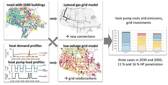
- The mutual investigation of power and natural gas distribution infrastructure for a whole town using a pipe and power-flow grid analysis.
- Deriving open models from a large number and different types of public data only, creating a highly diversified spatial and temporal resolution.
- Using a multi-perspective approach that considers electricity and natural gas grid investments, heat pump costs, and CO emissions for three cases.
2. Materials and Methods
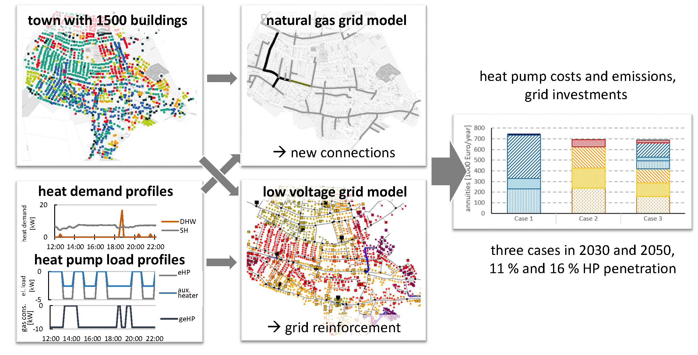
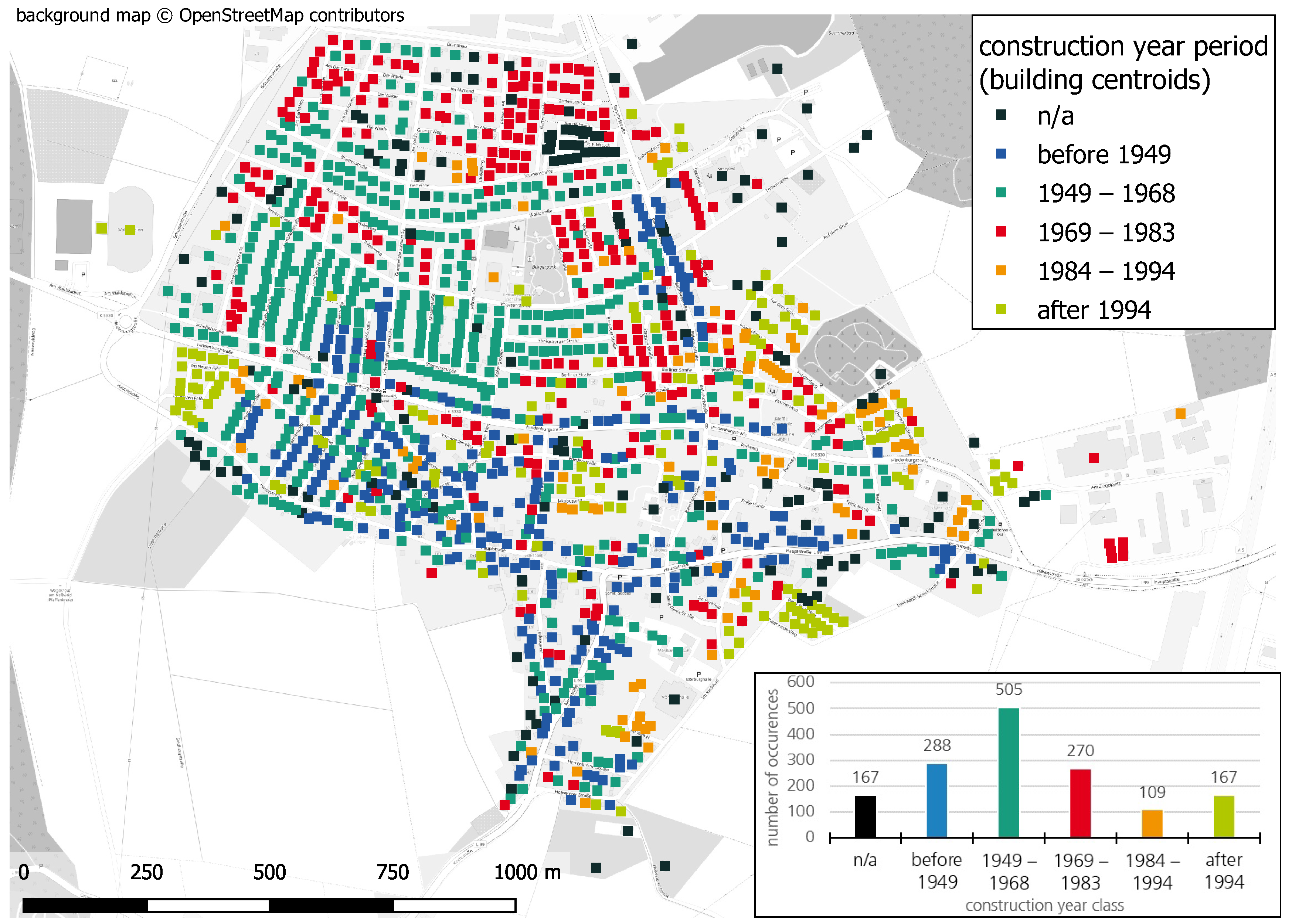
2.1. GIS-Based Information
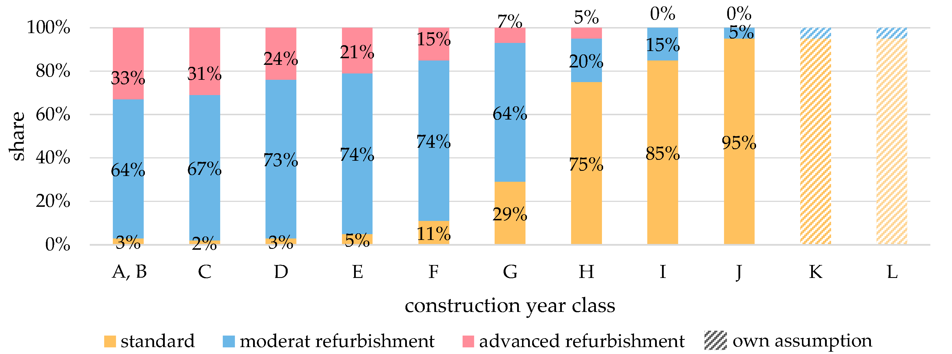
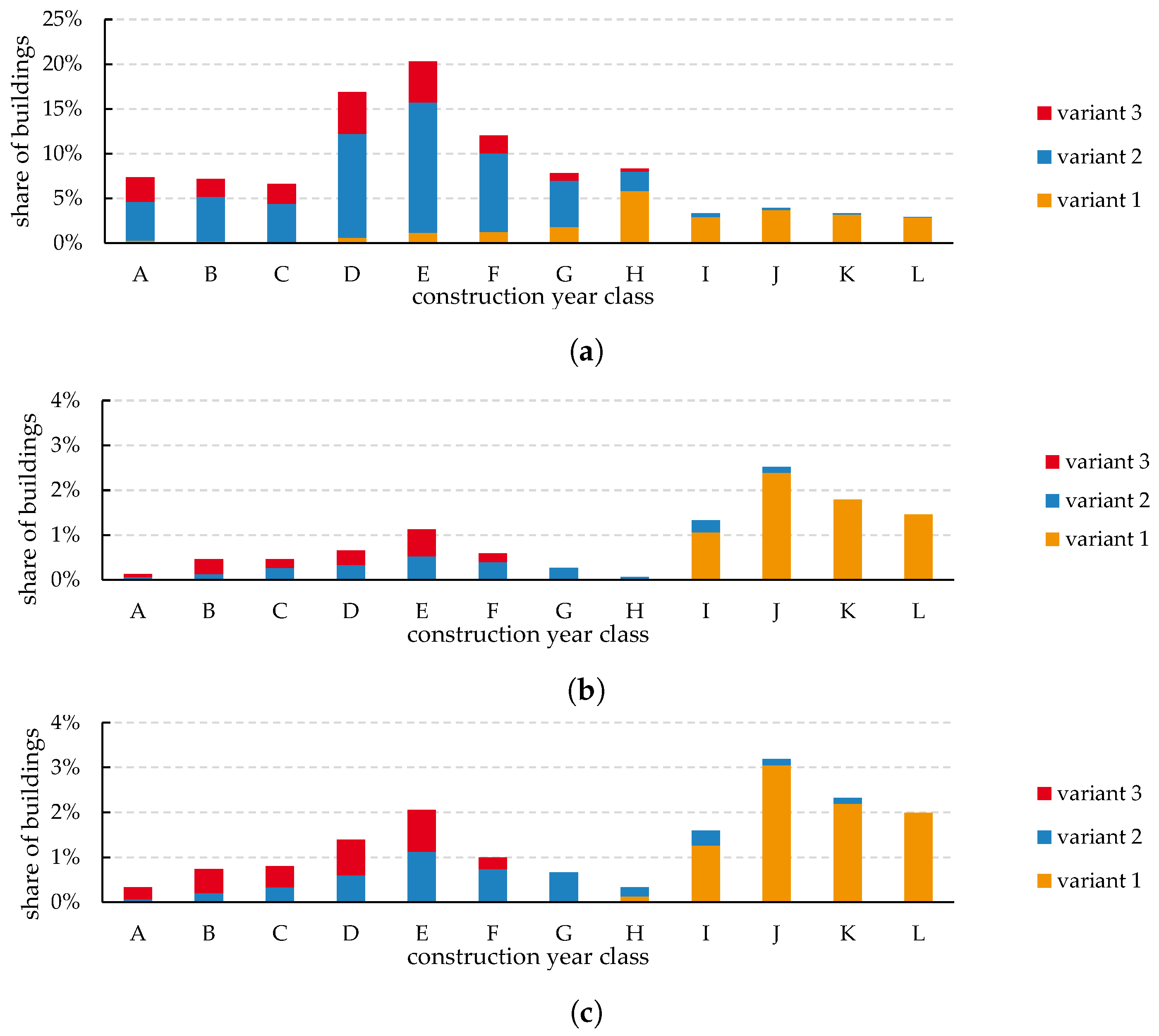
- Variant 1: “standard (no refurbishment).”
- Variant 2: “moderate refurbishment.”
- Variant 3: “advanced refurbishment.”
2.2. Class-Based Electrical and Thermal Load Profiles
2.3. GIS-Based Grid Connection Point Profiles
- Natural gas-fired boiler;
- Electric heat pumps with auxiliary heating coils (eHPs);
- Gas engine heat pumps (geHPs).
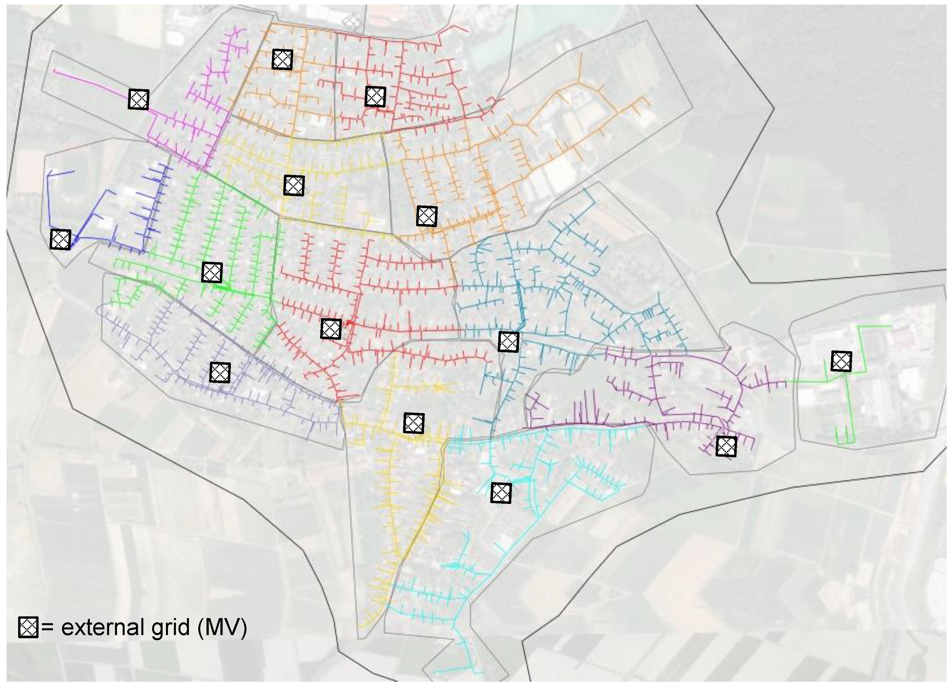
2.4. GIS-Based Grid Models
2.4.1. Low Voltage Power Grid Model
- Synthetic, because it is not based on a real DSO grid model;
- Example, because the main purpose is to illustrate different scenarios;
- Benchmark, because it is used to compare different scenarios by derived grid expansion costs.
- The street lines downloaded from OpenStreetMap are segmented into sets of points with 1 m distance and an individual ID, called grid-points, using the QGIS-plugin QChainage [81]. It is assumed that cables are routed along the streets and each house is assigned to its nearest grid-point using the extension NNJoin [82]. All grid-points that have no house assigned are deleted.
- The remaining grid-points are connected to their assigned houses by cables of type NAYY 4x50. To derive a preliminary grid structure, grid-points are connected to their nearest neighbor in the same street with less than 40 m distance by cables of the type NAYY 4x150. The parameters and locations of the MV/LV transformer stations are taken from the pandapower grid “MV Oberrhein”. All information is imported to PSS® Sincal to proceed with a graphical interface.
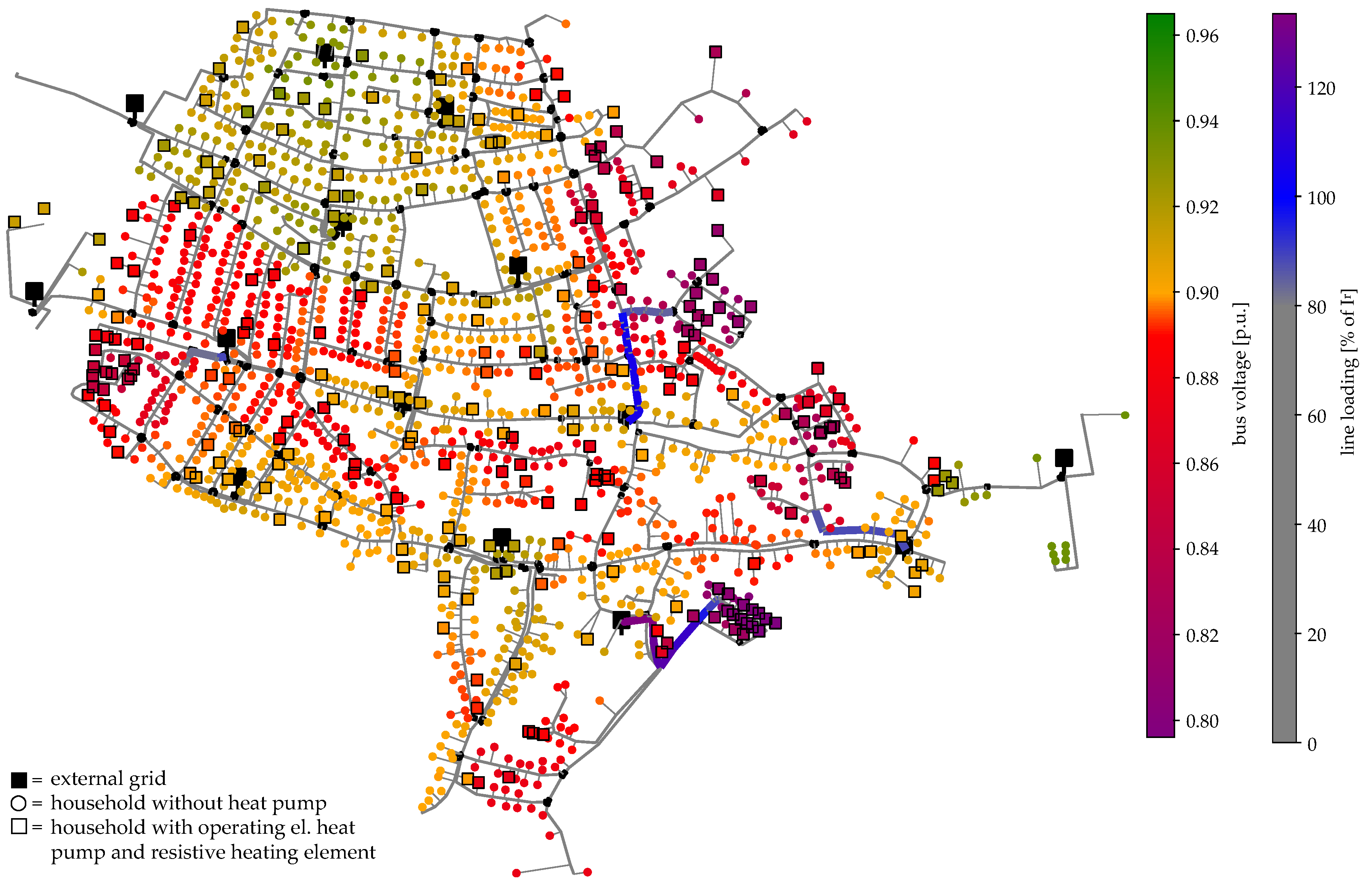
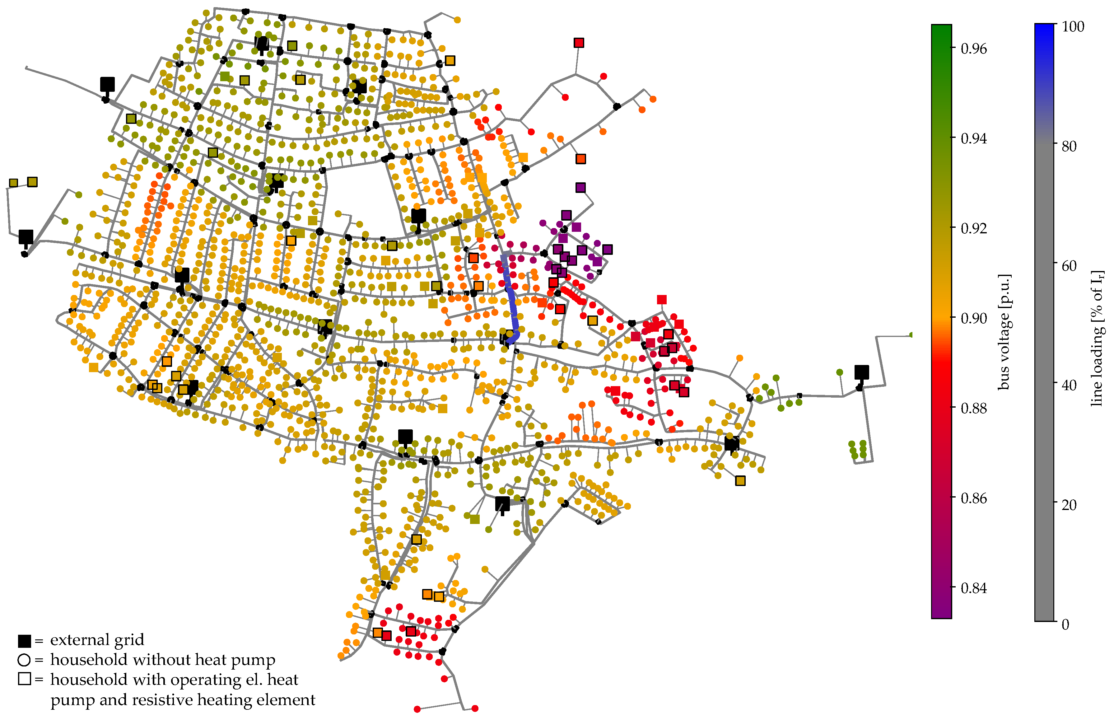
- The imported information is validated and existing errors due to the automated approach of grid generation are corrected manually. For each transformer, a supply area is chosen and the respective branches are connected by cables of type NAYY 4x150 to the LV-busbar of the transformer. Crossing points of many cables are equipped with switch cabinets. A radial topology without any galvanic connections between transformers is ensured by appropriate switch configuration. The result is shown in Figure 4.
- For each house, a peak load of kW and kVar is assumed, which represents a of 0.96. With these values, a load flow calculation is performed to make sure that the grid model is valid and the voltage and current of each cable, bus, and transformer stay within given limits. Limits are chosen to be 0.9–1.1 p.u. for bus voltages, 60% capacity for cables, and 130% for transformers (oil insulated) [83].
- If violations of given voltage and capacity limits are found at this stage, switch measure, direct connection to bus bars; or new, parallel cables are added until all restrictions are met.
- The Sincal-grid model is imported to pandapower and by using the integrated converter of pandapower-pro.
- The loads in pandapower are connected with the house data (construction year classes, the status of energetic refurbishment, household type) from Figure 2.
- Time-series of load profiles for each of the 1506 household loads are matched using one of the 2000 generated load profiles.
- A final load flow calculation for a whole year (all time-steps) is done to validate the grid and make sure all the voltage and currents are within the given limits.
2.4.2. Natural Gas Grid Model
- The raw network topology was derived from a map presented in [54].
- Detailed information such as pipe diameters and types was derived from the gas network operator’s online planning information platform [57] and was set in STANET® accordingly. The backbone of the gas system is made of pipes of the type 180 PE 100; all other pipes are of type 125 PE 100.
- The location of the city gate station (pressure regulator station) was taken from the route depicted in the land utilization plan [56] and assumed to provide a constant pressure of 1 bar. It was implemented as a constant pressure node in STANET®.
- The buildings and their types that were set in the electrical distribution grid model were imported to the gas distribution grid model.
- Linear connection pipes from houses to the nearest natural gas pipeline were created by using the STANET® function “Create house connection pipes”.
- The STANET® grid model was exported as a CSV-file and imported into pandapipes, an open-source Python package for pipe flow and network simulation [85], for further analysis, e.g., on different lengths of house connection pipes.
- Gas network capacity tests were conducted to find potential violations of the operation limits (flow velocity and nodal pressure). For these tests, it was assumed that all houses in the model were heated by gas boilers, except for those with an assigned heat pump. Then, time-series simulations were conducted in pandapipes. The highest gas flow velocity and the lowest nodal pressure per time step were logged.
2.5. GIS-Based Grid Expansion Planning
- Case 1 “electric”: All heat pumps are realized as eHPs.
- Case 2 “natural gas”: All heat pumps are realized as geHPs.
- Case 3 “mixed”: It is assumed that heat pumps are driven by gas engines for houses that are close to the gas grid (less than 67 m linear distance). Heat pumps in other houses are implemented as eHPs.
2.5.1. Allocation of Heat Pumps
2.5.2. Grid Analysis
2.5.3. Grid Reinforcement
- Replacing overloaded cables or cables that were upstream of voltage band violations by cables with increased diameter (NAYY 4x240).
- Adding parallel cables (NAYY 4x240) to replaced cables.

| Conductor | Costs | Reference | Depreciation Period |
|---|---|---|---|
| LV cable, NAYY 4x150 mm | 95,000 EUR/km | [87] | 40 years |
| LV cable, NAYY 4x240 mm | 114,000 EUR/km | calc. from [87,88] | 40 years |
| house connection gas pipe, DN 50 | 1488 EUR + 95 EUR/m | [89] | 45 years |
3. Results
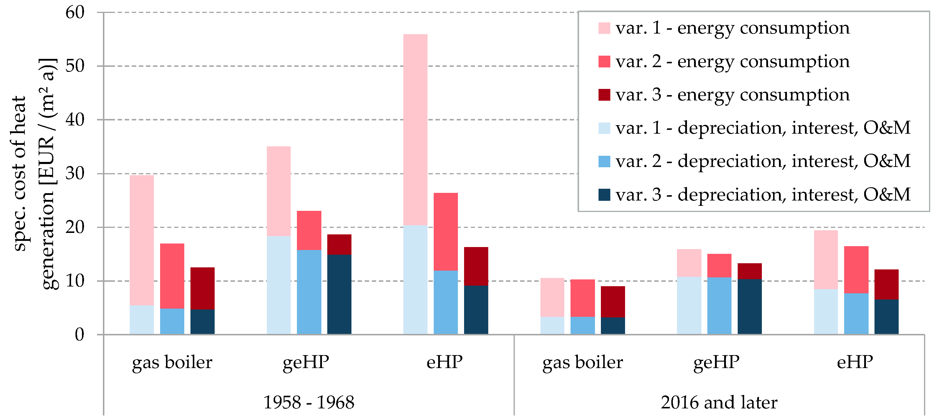
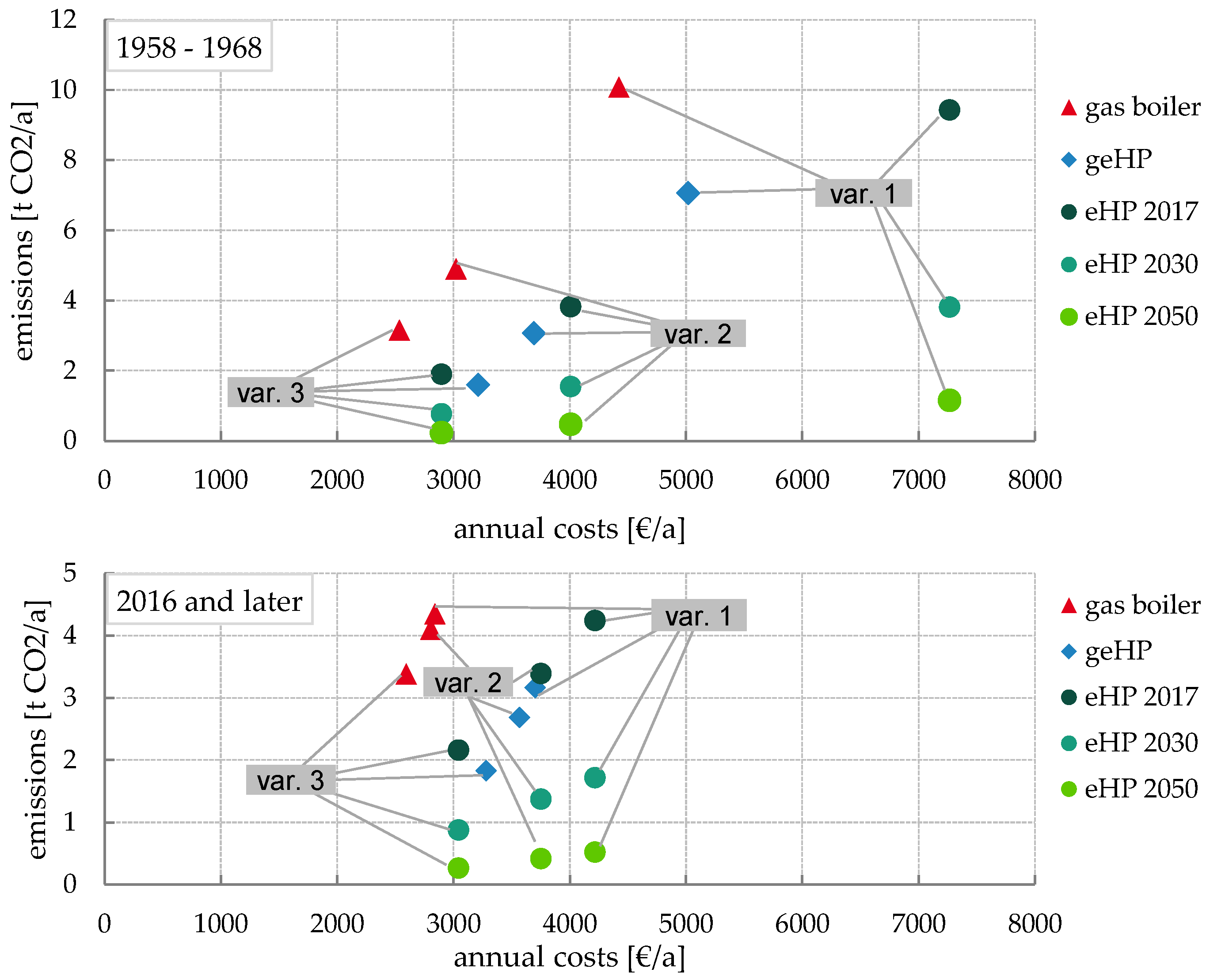
3.1. Costs and CO Emissions for Single Buildings and New Heating Systems
3.2. Cost and Emissions for Investigated Buildings in Schutterwald
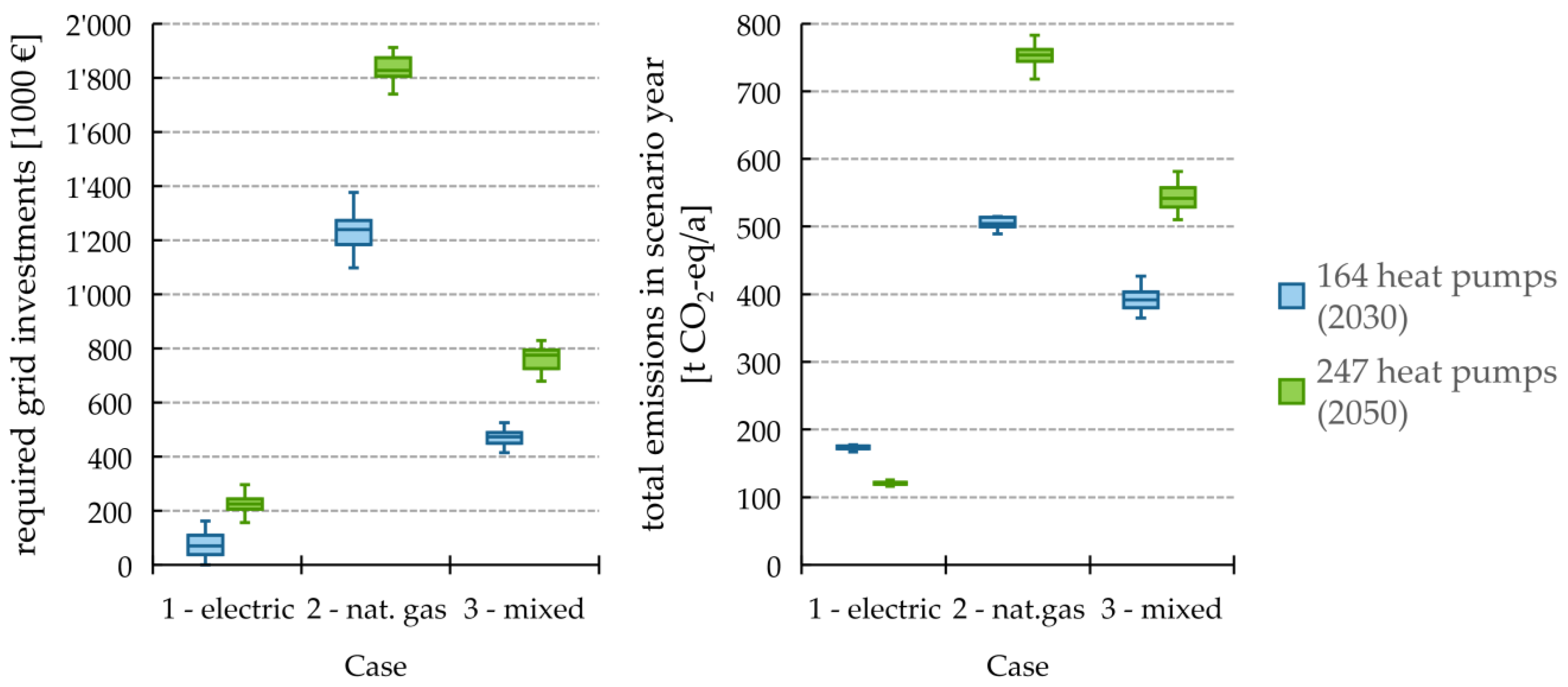
3.3. Required Grid Investments in the Gas and Power Grids
3.3.1. Case 1—Electric (eHPs)
3.3.2. Case 2—Natural Gas (geHP)
3.3.3. Case 3—Mixed (eHPs and geHPs)
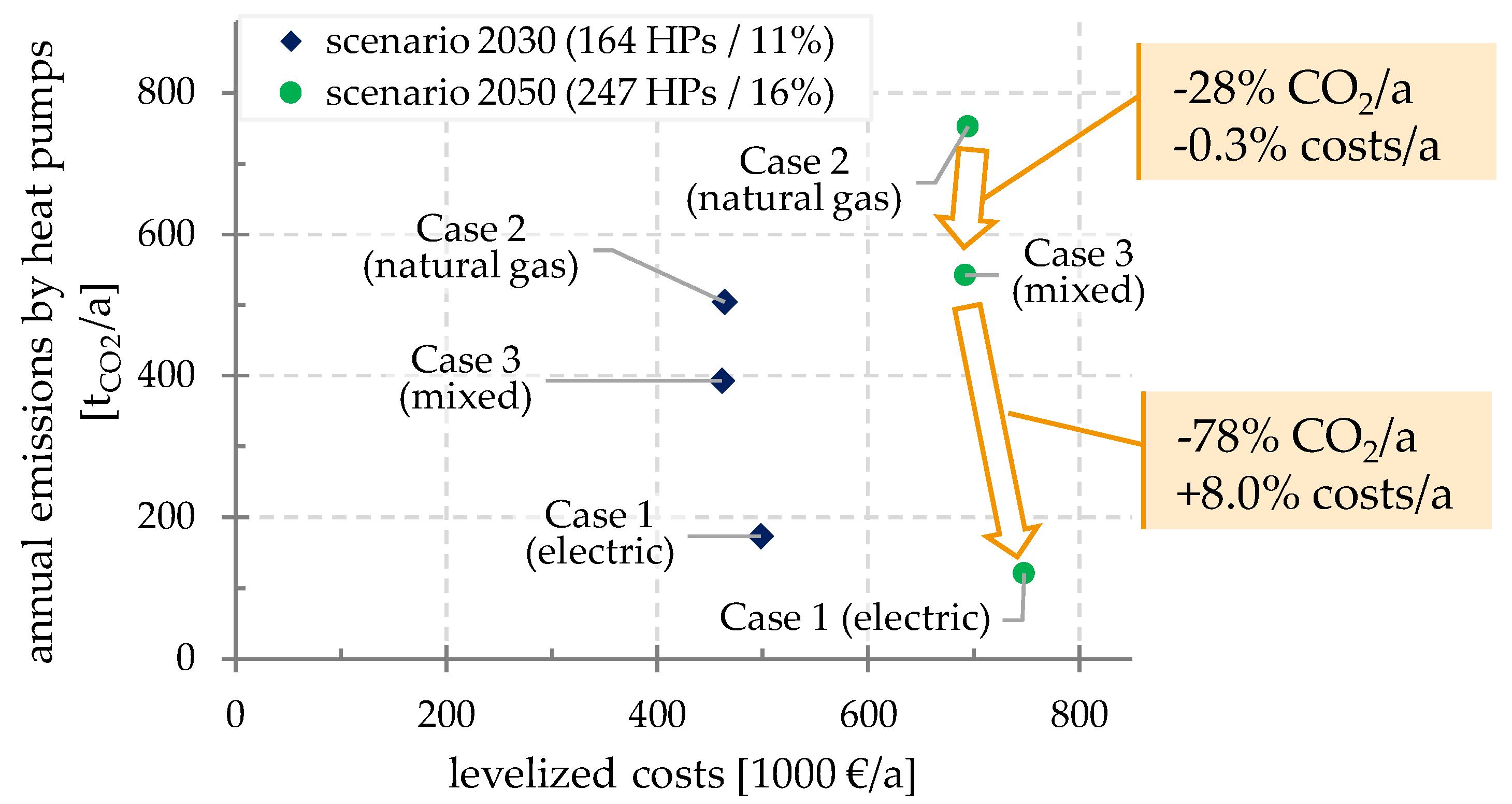
3.4. Combined Costs of Heat Supply and Grid Investments
4. Summary
4.1. Conclusions
- On the basis of a large number and different types of public data only, a low voltage and gas grid model with a highly diversified spatial resolution has been created for an example town and made available in the Supplementary Materials.
- We did a mutual investigation of power and natural gas distribution infrastructure for a whole town using a pipe and power-flow grid analysis.
- For all three cases, we investigated grid investments, heat pump costs, and CO emissions for a multi-perspective approach.
4.2. Discussion and Limitations
4.3. Further Research
Supplementary Materials
Author Contributions
Funding
Acknowledgments
Conflicts of Interest
Abbreviations
| aux. | auxiliary |
| CAPEX | capital expenditure |
| CHP | combined heat and power |
| cons. | consumption |
| constr. | construction |
| COP | coefficient of performance |
| DHW | domestic hot water |
| DSO | distribution system operator |
| eHP, eHPs | electric heat pump, electric heat pumps |
| el. | electricity |
| EMF | emission factor |
| geHP, geHPs | gas engine heat pump, gas engine heat pumps |
| Hh., hh | household |
| NZEB | nearly zero-energy building |
| O&M | operation and maintenance costs |
| OSM | OpenStreetMap |
| prod. | production |
| PV | photovoltaic |
| SH | space heating |
| WACC | weighted average cost of capital |
| YTM | yield to maturity |
Appendix A. Supplementary Tables
| Household Type | Space Heating [kWh] | DHW [kWh] | El. Hh. Devices [kWh] |
|---|---|---|---|
| single, employed | 19,618 | 847 | 2263 |
| single, retired | 19,579 | 869 | 1912 |
| couple, employed, no children | 18,620 | 1707 | 3281 |
| couple, employed, 1 child | 17,827 | 2578 | 4207 |
| couple, employed, 2 children | 16,923 | 3455 | 4842 |
| Constr. Year Class | Energy Refurb. Variant | Heat Demand [kWh/a] | El. Cons. eHP [kWh/a] | Heat Prod. eHP [kWh/a] | Annual COP (eHP Only) | El. Cons. Aux. Heating Coil [kWh/a] | Annual COP (System of eHP + Coil ) |
|---|---|---|---|---|---|---|---|
| A | 1 | 66,975 | 30,725 | 73,422 | 2.39 | 1856 | 2.31 |
| 2 | 22,812 | 8847 | 26,082 | 2.95 | 739 | 2.80 | |
| 3 | 13,557 | 4116 | 16,051 | 3.90 | 488 | 3.59 | |
| B | 1 | 40,965 | 19,244 | 46,207 | 2.40 | 1164 | 2.32 |
| 2 | 15,088 | 6035 | 17,938 | 2.97 | 499 | 2.82 | |
| 3 | 9667 | 3030 | 12,027 | 3.97 | 372 | 3.64 | |
| C | 1 | 59,076 | 27,184 | 65,014 | 2.39 | 1679 | 2.31 |
| 2 | 29,102 | 11,287 | 33,219 | 2.94 | 922 | 2.80 | |
| 3 | 19,762 | 5857 | 22,555 | 3.85 | 712 | 3.54 | |
| D | 1 | 32,674 | 15,403 | 37,145 | 2.41 | 884 | 2.33 |
| 2 | 14,130 | 5678 | 16,942 | 2.98 | 426 | 2.85 | |
| 3 | 7991 | 2577 | 10,311 | 4.00 | 287 | 3.70 | |
| E | 1 | 35,026 | 16,582 | 39,929 | 2.41 | 976 | 2.33 |
| 2 | 16,639 | 6577 | 19,554 | 2.97 | 549 | 2.82 | |
| 3 | 10,125 | 3159 | 12,517 | 3.96 | 384 | 3.64 | |
| F | 1 | 36,594 | 17,142 | 41,238 | 2.41 | 1043 | 2.33 |
| 2 | 17,809 | 7041 | 20,796 | 2.95 | 568 | 2.81 | |
| 3 | 12,543 | 3843 | 15,033 | 3.91 | 491 | 3.58 | |
| G | 1 | 29,902 | 14,126 | 34,050 | 2.41 | 853 | 2.33 |
| 2 | 17,219 | 6803 | 20,166 | 2.96 | 572 | 2.81 | |
| 3 | 12,327 | 3782 | 14,843 | 3.92 | 474 | 3.60 | |
| H | 1 | 24,728 | 11,810 | 28,476 | 2.41 | 674 | 2.34 |
| 2 | 16,176 | 6428 | 19,071 | 2.97 | 528 | 2.82 | |
| 3 | 10,589 | 3298 | 12,964 | 3.93 | 393 | 3.62 | |
| I | 1 | 15,938 | 7821 | 18,997 | 2.43 | 460 | 2.35 |
| 2 | 13,400 | 5453 | 16,252 | 2.98 | 413 | 2.84 | |
| 3 | 9116 | 2865 | 11,396 | 3.98 | 367 | 3.64 | |
| J | 1 | 13,988 | 6932 | 16,858 | 2.43 | 436 | 2.35 |
| 2 | 12,678 | 5168 | 15,487 | 3.00 | 404 | 2.85 | |
| 3 | 10,318 | 3193 | 12,683 | 3.97 | 386 | 3.65 | |
| K | 1 | 18,232 | 8839 | 21,419 | 2.42 | 528 | 2.34 |
| 2 | 16,358 | 6513 | 19,321 | 2.97 | 519 | 2.82 | |
| 3 | 11,788 | 3631 | 14,335 | 3.95 | 442 | 3.63 | |
| L | 1 | 15,178 | 7448 | 18,140 | 2.44 | 444 | 2.35 |
| 2 | 14,490 | 5826 | 17,331 | 2.97 | 482 | 2.82 | |
| 3 | 11,611 | 3602 | 14,166 | 3.93 | 423 | 3.62 |
| Constr. Year Class | Energy Refurb. Variant | Heat Demand [kWh/a] | Fuel Cons. [kWh/a] | Heat Prod. [kWh/a] | Primary Energy Ratio |
|---|---|---|---|---|---|
| A | 1 | 66,975 | 60,189 | 75,524 | 1.25 |
| 2 | 22,812 | 18,575 | 26,478 | 1.43 | |
| 3 | 13,557 | 9514 | 16,451 | 1.73 | |
| B | 1 | 40,965 | 37,224 | 46,770 | 1.26 |
| 2 | 15,088 | 12,633 | 18,148 | 1.44 | |
| 3 | 9667 | 6893 | 12,007 | 1.74 | |
| C | 1 | 59,076 | 53,214 | 66,817 | 1.26 |
| 2 | 29,102 | 23,615 | 33,590 | 1.42 | |
| 3 | 19,762 | 13,692 | 23,420 | 1.71 | |
| D | 1 | 32,674 | 29,579 | 37,250 | 1.26 |
| 2 | 14,130 | 11,768 | 16,942 | 1.44 | |
| 3 | 7991 | 5715 | 9970 | 1.74 | |
| E | 1 | 35,026 | 31,760 | 39,894 | 1.26 |
| 2 | 16,639 | 13,787 | 19,799 | 1.44 | |
| 3 | 10,125 | 7205 | 12,531 | 1.74 | |
| F | 1 | 36,594 | 33,183 | 41,760 | 1.26 |
| 2 | 17,809 | 14,788 | 21,165 | 1.43 | |
| 3 | 12,543 | 8878 | 15,352 | 1.73 | |
| G | 1 | 29,902 | 27,105 | 34,096 | 1.26 |
| 2 | 17,219 | 14,342 | 20,591 | 1.44 | |
| 3 | 12,327 | 8686 | 15,003 | 1.73 | |
| H | 1 | 24,728 | 22,614 | 28,495 | 1.26 |
| 2 | 16,176 | 13,433 | 19,252 | 1.43 | |
| 3 | 10,589 | 7501 | 12,983 | 1.73 | |
| I | 1 | 15,938 | 14,928 | 18,894 | 1.27 |
| 2 | 13,400 | 11,237 | 16,138 | 1.44 | |
| 3 | 9116 | 6553 | 11,470 | 1.75 | |
| J | 1 | 13,988 | 13,243 | 16,784 | 1.27 |
| 2 | 12,678 | 10,661 | 15,353 | 1.44 | |
| 3 | 10,318 | 7275 | 12,685 | 1.74 | |
| K | 1 | 18,232 | 16,937 | 21,404 | 1.26 |
| 2 | 16,358 | 13,608 | 19,523 | 1.43 | |
| 3 | 11,788 | 8287 | 14,389 | 1.74 | |
| L | 1 | 15,178 | 14,219 | 18,039 | 1.27 |
| 2 | 14,490 | 12,069 | 17,306 | 1.43 | |
| 3 | 11,611 | 8209 | 14,224 | 1.73 |
| Existing State (Var. 1) | Usual Refurbish- ment (Var. 2) | Adv. Refurbish- ment (Var. 3) | Information: EMF [g/kWh] | ||||
|---|---|---|---|---|---|---|---|
| Costs | Emissions | Costs | Emissions | Costs | Emissions | ||
| oil boiler | 5311 | 13.7 | 3386 | 6.6 | 2714 | 4.1 | 266 |
| gas boiler | 4873 | 10.8 | 3197 | 5.0 | 2625 | 3.2 | 202 |
| geHP | 5320 | 7.5 | 3798 | 3.1 | 3263 | 1.6 | 202 |
| eHP 2017 | 7809 | 10.9 | 4196 | 4.3 | 2983 | 2.1 | 537 |
| eHP 2030 | 7809 | 4.4 | 4196 | 1.7 | 2983 | 0.9 | 141 |
| eHP 2050 | 7809 | 1.3 | 4196 | 0.5 | 2983 | 0.3 | 66 |
| National Minimum Requirement (Var. 1) | Ambitious Standard/ NZEB (Var. 2) | Advanced Refurbishment (Var. 3) | Information: EMF [g/kWh] | ||||
|---|---|---|---|---|---|---|---|
| Costs | Emissions | Costs | Emissions | Costs | Emissions | ||
| oil boiler | 3146 | 5.7 | 3114 | 5.6 | 2818 | 4.5 | 266 |
| gas boiler | 2987 | 4.5 | 2962 | 4.3 | 2713 | 3.5 | 202 |
| geHP | 3809 | 3.2 | 3669 | 2.8 | 3345 | 1.9 | 202 |
| eHP 2017 | 4412 | 4.7 | 3926 | 3.8 | 3146 | 2.4 | 537 |
| eHP 2030 | 4412 | 1.9 | 3926 | 1.6 | 3146 | 1.0 | 141 |
| eHP 2050 | 4412 | 0.6 | 3926 | 0.5 | 3146 | 0.3 | 66 |
| Year | Number of Heat Pumps | Case | Mean | Min | Q | Q | Q | Max | |
|---|---|---|---|---|---|---|---|---|---|
| 2030 | 164 | 1 - electric | 494 | 6 | 480 | 491 | 494 | 500 | 502 |
| 2 - natural gas | 416 | 3 | 411 | 415 | 416 | 419 | 419 | ||
| 3 - mixed | 443 | 3 | 438 | 440 | 442 | 446 | 448 | ||
| 2050 | 247 | 1 - electric | 736 | 11 | 707 | 730 | 737 | 741 | 759 |
| 2 - natural gas | 624 | 5 | 613 | 622 | 624 | 627 | 634 | ||
| 3 - mixed | 662 | 6 | 646 | 659 | 663 | 667 | 672 |
| Year | Number of Heat Pumps | Case | Mean | Min | Q | Q | Q | Max | |
|---|---|---|---|---|---|---|---|---|---|
| 2030 | 164 | 1 - electric | 76 | 46 | 0 | 38 | 69 | 109 | 162 |
| 2 - natural gas | 1237 | 74 | 1097 | 1184 | 1238 | 1273 | 1376 | ||
| 3 - mixed | 473 | 30 | 415 | 450 | 472 | 489 | 526 | ||
| 2050 | 247 | 1 - electric | 223 | 36 | 157 | 205 | 225 | 244 | 296 |
| 2 - natural gas | 1830 | 46 | 1740 | 1805 | 1828 | 1,873 | 1912 | ||
| 3 - mixed | 757 | 44 | 679 | 725 | 775 | 794 | 829 |
| Year | Number of Heat Pumps | Case | Mean | Min | Q | Q | Q | Max | |
|---|---|---|---|---|---|---|---|---|---|
| 2030 | 164 | 1 - electric | 173 | 3 | 167 | 172 | 173 | 176 | 177 |
| 2 - natural gas | 505 | 8 | 489 | 501 | 504 | 513 | 515 | ||
| 3 - mixed | 392 | 16 | 365 | 380 | 392 | 403 | 427 | ||
| 2050 | 247 | 1 - electric | 120 | 2 | 114 | 119 | 121 | 122 | 125 |
| 2 - natural gas | 753 | 14 | 718 | 745 | 753 | 761 | 783 | ||
| 3 - mixed | 543 | 19 | 510 | 530 | 542 | 557 | 582 |
| Parameter | Value | Reference |
|---|---|---|
| discount rate households | 2.67 % | average of [13,71,72] |
| equity interest rate DSO | 6.91 % | [92] |
| debt interest rate DSO | 1.33 % | 10 year avg. of YTM on German bearer debentures (2009–’18) [93] |
| equity ratio DSO | 52.73 % | [94] |
| discount rate DSO (WACC) | 4.27 % | own calculation |
References
- European Parliament; Council of the European Union. Directive (EU) 2018/2002 of the European Parliament and of the Council of 11 December 2018 amending Directive 2012/27/EU on energy efficiency. Off. J. Eur. Union 2018, 328, 210–230. [Google Scholar]
- Erbach, G. Understanding Energy Efficiency; European Parliamentary Research Service: Brussels, Belgium, 2015. [Google Scholar]
- German Federal Ministry for the Environment, Nature Conservation, Building and Nuclear Safety (BMUB). Climate Action Plan 2050: Principles and Goals of the German Government’s Climate Policy; BMUB, Division KI I 1: Berlin, Germany, 2016.
- Federal Ministry for Economic Affairs and Energy (BMWi). The Energy of the Future: Second Progress Report on the Energy Transition. Reporting Year 2017; BMWi, Public Relations Division: Berlin, Germany, 2019.
- Fraunhofer IWES; Fraunhofer IBP. Heat Transition 2030; Agora Energiewende: Berlin, Germany, 2017. [Google Scholar]
- von Appen, J. Sizing and Operation of Residential Photovoltaic Systems in Combination with Battery Storage Systems and Heat Pumps: Multi-Actor Optimization Models and Case Studies. Ph.D. Thesis, University Kassel, Kassel, Germany, 2018. [Google Scholar]
- von Appen, J.; Braun, M. Sizing and improved grid integration of residential PV systems with heat pumps and battery storage systems. IEEE Trans. Energy Convers. 2019, 34, 562–571. [Google Scholar] [CrossRef]
- Scheidler, A.; Bolgaryn, R.; Ulffers, J.; Dasenbrock, J.; Horst, D.; Gauglitz, P.; Pape, C.; Becker, H. DER Integration Study for the German State of Hesse—Methodology and Key Results. In Proceedings of the 25th International Conference on Electricity Distribution, Madrid, Spain, 3–6 June 2019; CIRED: Madrid, Spain, 2019; pp. 1–5. [Google Scholar] [CrossRef]
- Guelpa, E.; Bischi, A.; Verda, V.; Chertkov, M.; Lund, H. Towards future infrastructures for sustainable multi-energy systems: A review. Energy 2019, 184, 2–21. [Google Scholar] [CrossRef]
- Mancarella, P. MES (multi-energy systems): An overview of concepts and evaluation models. Energy 2014, 65, 1–17. [Google Scholar] [CrossRef]
- Prina, M.G.; Manzolini, G.; Moser, D.; Nastasi, B.; Sparber, W. Classification and challenges of bottom-up energy system models—A review. Renew. Sust. Energ. Rev. 2020, 129, 109917. [Google Scholar] [CrossRef]
- D’Agostino, D.; Mazzarella, L. What is a Nearly zero energy building? Overview, implementation and comparison of definitions. J. Build. Eng. 2019, 21, 200–212. [Google Scholar] [CrossRef]
- Ifeu, Fraunhofer IEE, Consentec. Building Sector Efficiency: A Crucial Component of the Energy Transition; Agora Energiewende: Berlin, Germany, 2018. [Google Scholar]
- Webb, A.L. Energy retrofits in historic and traditional buildings: A review of problems and methods. Renew. Sust. Energ. Rev. 2017, 77, 748–759. [Google Scholar] [CrossRef]
- de Santoli, L.; Lo Basso, G.; Nastasi, B. Innovative Hybrid CHP systems for high temperature heating plant in existing buildings. Energy Procedia 2017, 133, 207–218. [Google Scholar] [CrossRef]
- Kneiske, T.M.; Braun, M.; Hidalgo-Rodriguez, D.I. A new combined control algorithm for PV-CHP hybrid systems. Appl. Energy 2018, 210, 964–973. [Google Scholar] [CrossRef]
- Kneiske, T.M.; Niedermeyer, F.; Boelling, C. Testing a model predictive control algorithm for a PV-CHP hybrid system on a laboratory test-bench. Appl. Energy 2019, 242, 121–137. [Google Scholar] [CrossRef]
- Kneiske, T.M.; Braun, M. Flexibility potentials of a combined use of heat storages and batteries in PV-CHP hybrid systems. Energy Procedia 2017, 135, 482–495. [Google Scholar] [CrossRef]
- Lee, Z.; Lee, K.; Choi, S.; Park, S. Combustion and Emission Characteristics of an LNG Engine for Heat Pumps. Energies 2015, 8, 13864–13878. [Google Scholar] [CrossRef] [Green Version]
- Hepbasli, A.; Erbay, Z.; Icier, F.; Colak, N.; Hancioglu, E. A review of gas engine driven heat pumps (GEHPs) for residential and industrial applications. Renew. Sust. Energ. Rev. 2009, 13, 85–99. [Google Scholar] [CrossRef]
- Elgendy, E. Analysis of Energy Efficiency of Gas Driven Heat Pumps. Ph.D. Thesis, Otto-von-Guericke-Universität Magdeburg, Magdeburg, Germany, 2011. [Google Scholar]
- Elgendy, E.; Schmidt, J. Optimum utilization of recovered heat of a gas engine heat pump used for water heating at low air temperature. Energy Build. 2014, 80, 375–383. [Google Scholar] [CrossRef]
- Protopapadaki, C.; Saelens, D. Heat pump and PV impact on residential low-voltage distribution grids as a function of building and district properties. Appl. Energy 2017, 192, 268–281. [Google Scholar] [CrossRef]
- Protopapadaki, C.; Saelens, D. Corrigendum to “Heat pump and PV impact on residential low-voltage distribution grids as a function of building and district properties” [Appl. Energy 192 (2017) 268–281]. Appl. Energy 2017, 205, 1605–1608. [Google Scholar] [CrossRef] [Green Version]
- Sichilalu, S.; Xia, X.; Zhang, J. Optimal Scheduling Strategy for a Grid-connected Photovoltaic System for Heat Pump Water Heaters. Energy Procedia 2014, 61, 1511–1514. [Google Scholar] [CrossRef] [Green Version]
- Carvalho, A.D.; Moura, P.; Vaz, G.C.; de Almeida, A.T. Ground source heat pumps as high efficient solutions for building space conditioning and for integration in smart grids. Energy Convers. Manag. 2015, 103, 991–1007. [Google Scholar] [CrossRef]
- Roselli, C.; Diglio, G.; Sasso, M.; Tariello, F. A novel energy index to assess the impact of a solar PV-based ground source heat pump on the power grid. Renew. Energy 2019, 143, 488–500. [Google Scholar] [CrossRef]
- Fischer, D.; Madani, H. On heat pumps in smart grids: A review. Renew. Sust. Energ. Rev. 2017, 70, 342–357. [Google Scholar] [CrossRef] [Green Version]
- Longfei, M.A.; Long, G.; Li, X.; Chen, Y.; Gong, C.; Wang, W.; Xu, H. Research on influence of large-scale air-source heat pump start-up characteristics to power grid. In Proceedings of the 2017 IEEE Conference on Energy Internet and Energy System Integration (EI2), Beijing, China, 26–28 November 2017; pp. 1–4. [Google Scholar] [CrossRef]
- Bernath, C.; Deac, G.; Sensfuß, F. Influence of heat pumps on renewable electricity integration: Germany in a European context. Energy Strategy Rev. 2019, 26, 100389. [Google Scholar] [CrossRef]
- Klyapovskiy, S.; You, S.; Cai, H.; Bindner, H.W. Incorporate flexibility in distribution grid planning through a framework solution. Int. J. Electr. Power Energy Syst. 2019, 111, 66–78. [Google Scholar] [CrossRef]
- Thurner, L.; Scheidler, A.; Schäfer, F.; Menke, J.H.; Dollichon, J.; Meier, F.; Meinecke, S.; Braun, M. Pandapower—An Open Source Python Tool for Convenient Modeling, Analysis and Optimization of Electric Power Systems. IEEE Trans. Power Syst. 2018, 33, 6510–6521. [Google Scholar] [CrossRef] [Green Version]
- Scheidler, A.; Thurner, L.; Braun, M. Heuristic optimisation for automated distribution system planning in network integration studies. IET Renew. Power Gener. 2018, 12, 530–538. [Google Scholar] [CrossRef] [Green Version]
- Schaefer, F.; Menke, J.H.; Braun, M. Comparison of Meta-Heuristics for the Planning of Meshed Power Systems. arXiv 2020, arXiv:2002.03619. [Google Scholar]
- Sieberichs, M.; Ashrafuzzaman, R.; Moser, A. Implications of optimization strategies on expansion planning in medium- and low-voltage networks. In Proceedings of the 2017 6th International Conference on Clean Electrical Power (ICCEP), Santa Margherita Ligure, Italy, 27–29 June 2017; pp. 236–241. [Google Scholar] [CrossRef]
- Bolgaryn, R.; Scheidler, A.; Braun, M. Combined Planning of Medium and Low Voltage Grids. In Proceedings of the 2019 IEEE Milan PowerTech, Milan, Italy, 23–27 June 2019; pp. 1–6. [Google Scholar] [CrossRef]
- Büchner, D.; Thurner, L.; Kneiske, T.M.; Braun, M. Automated Network Planning including an Asset Management Strategy: Conference Center, Bonn. In Proceedings of the International ETG Congress 2017, Bonn, Germany, 28–29 November 2017; VDE Verlag: Berlin, Germany, 2017; Volume 155. [Google Scholar]
- Yan, J.; Zhou, K.; Deng, C.; Huang, J. A GIS Based Service-Oriented Power Grid Intelligent Planning System. In Proceedings of the 2011 Asia-Pacific Power and Energy Engineering Conference, Wuhan, China, 25–28 March 2011; pp. 1–4. [Google Scholar] [CrossRef]
- Mueller, F.; Zimmerlin, M.; de Jongh, S.; Suriyah, M.R.; Leibfried, T. Comparison of multi-timestep Optimization Methods for Gas Distribution Grids. In Proceedings of the 2019 54th International Universities Power Engineering Conference (UPEC), Bucharest, Romania, 3–6 September 2019; pp. 1–6. [Google Scholar] [CrossRef]
- Then, D.; Spalthoff, C.; Bauer, J.; Kneiske, T.M.; Braun, M. Impact of Natural Gas Distribution Network Structure and Operator Strategies on Grid Economy in Face of Decreasing Demand. Energies 2020, 13, 664. [Google Scholar] [CrossRef] [Green Version]
- Then, D.; Hein, P.; Kneiske, T.M.; Braun, M. Analysis of Dependencies between Gas and Electricity Distribution Grid Planning and Building Energy Retrofit Decisions. Sustainability 2020, 12, 5315. [Google Scholar] [CrossRef]
- Khani, H.; El-Taweel, N.A.; Farag, H.E.Z. Power Loss Alleviation in Integrated Power and Natural Gas Distribution Grids. IEEE Trans. Ind. Informat. 2019, 15, 6220–6230. [Google Scholar] [CrossRef]
- Shao, C.; Shahidehpour, M.; Wang, X.; Wang, X.; Wang, B. Integrated Planning of Electricity and Natural Gas Transportation Systems for Enhancing the Power Grid Resilience. IEEE Trans. Power Syst. 2017, 32, 4418–4429. [Google Scholar] [CrossRef]
- Drauz, S.R.; Spalthoff, C.; Würtenberg, M.; Kneikse, T.M.; Braun, M. A modular approach for co-simulations of integrated multi-energy systems: Coupling multi-energy grids in existing environments of grid planning operation tools. In Proceedings of the 2018 Workshop on Modeling and Simulation of Cyber-Physical Energy Systems (MSCPES), Porto, Portugal, 10 April 2018; pp. 1–6. [Google Scholar] [CrossRef]
- Pambour, K.; Cakir Erdener, B.; Bolado-Lavin, R.; Dijkema, G. Development of a Simulation Framework for Analyzing Security of Supply in Integrated Gas and Electric Power Systems. Appl. Sci. 2017, 7, 47. [Google Scholar] [CrossRef] [Green Version]
- Farrokhifar, M.; Nie, Y.; Pozo, D. Energy systems planning: A survey on models for integrated power and natural gas networks coordination. Appl. Energy 2020, 262, 114567. [Google Scholar] [CrossRef]
- Barati, F.; Seifi, H.; Nateghi, A.; Sepasian, M.S.; Shafie-khah, M.; Catalão, J.P.S. An integrated generation, transmission and Natural Gas Grid Expansion Planning approach for large scale systems. In Proceedings of the 2015 IEEE Power Energy Society General Meeting, Denver, CO, USA, 26–30 July 2015; pp. 1–5. [Google Scholar] [CrossRef]
- Talebi, A.; Sadeghi-Yazdankhah, A.; Mirzaei, M.A.; Mohammadi-Ivatloo, B. Co-optimization of Electricity and Natural Gas Networks Considering AC Constraints and Natural Gas Storage. In Proceedings of the 2018 Smart Grid Conference (SGC), Sanandaj, Iran, 28–29 November 2018; pp. 1–6. [Google Scholar] [CrossRef]
- Jooshaki, M.; Abbaspour, A.; Fotuhi-Firuzabad, M.; Moeini-Aghtaie, M.; Lehtonen, M. Multistage Expansion Co-Planning of Integrated Natural Gas and Electricity Distribution Systems. Energies 2019, 12, 1020. [Google Scholar] [CrossRef] [Green Version]
- Alhamwi, A.; Medjroubi, W.; Vogt, T.; Agert, C. FlexiGIS: An open source GIS-based platform for the optimisation of flexibility options in urban energy systems. Energy Procedia 2018, 152, 941–946. [Google Scholar] [CrossRef]
- Alhamwi, A.; Medjroubi, W.; Vogt, T.; Agert, C. GIS-based urban energy systems models and tools: Introducing a model for the optimisation of flexibilisation technologies in urban areas. Appl. Energy 2017, 191, 1–9. [Google Scholar] [CrossRef]
- Alhamwi, A.; Medjroubi, W.; Vogt, T.; Agert, C. Development of a GIS-based platform for the allocation and optimisation of distributed storage in urban energy systems. Appl. Energy 2019, 251, 113360. [Google Scholar] [CrossRef]
- OpenStreetMap: Database Contents License (DbCL) 1.0. Available online: http://www.openstreetmap.org/ (accessed on 2 January 2019).
- Weiß, N.; Krecher, M. Energiepotenzialstudie Gemeinde Schutterwald; Badenova AG & Co. KG: Freiburg, Germany, 2014. [Google Scholar]
- Walberg, D.; Holz, A.; Gniechwitz, T.; Schulze, T. Wohnungsbau in Deutschland-2011-Modernisierung oder Bestandsersatz: Studie zum Zustand und der Zukunftsfähigkeit des Deutschen Kleinen Wohnungsbaus: Band I Textband; Arbeitsgemeinschaft für Zeitgemäßes Bauen: Kiel, Germany, 2011. [Google Scholar]
- Verwaltungsgemeinschaft Offenburg. Flächennutzungsplan Juli 2009: Blatt 2/West; Voegele + Gerhardt Freie Stadtplaner und Architekten DWB SRL BDA: Offenburg, Germany; Karlsruhe, Germany, 2009. [Google Scholar]
- planSERVICE: Leitungsauskunft Online. Available online: https://planservice.regiodata-service.de/ (accessed on 17 May 2019).
- Institut Wohnen und Umwelt. TABULA—Entwicklung von Gebäudetypologien zur Energetischen Bewertung des Wohngebäudebestands in 13 Europäischen Ländern: Supplementary Data Tables Appendix C. Available online: https://www.iwu.de/fileadmin/user_upload/dateien/energie/werkzeuge/TABULA-Analyses_DE-Typology_DataTables.zip (accessed on 15 June 2019).
- Loga, T.; Stein, B.; Diefenbach, N.; Born, R. Deutsche Wohngebäudetypologie: Beispielhafte Maßnahmen zur Verbesserung der Energieeffizienz von Typischen Wohngebäuden, 2nd ed.; Institut Wohnen und Umwelt (IWU): Darmstadt, Germany, 2015. [Google Scholar]
- Institut Wohnen und Umwelt (IWU). DE Germany—Country Page: Residential Building Typology. Available online: https://episcope.eu/building-typology/country/de/ (accessed on 17 February 2020).
- Statistisches Landesamt Baden-Württemberg. Bevölkerung und Haushalte: Gemeinde Schutterwald am 9. Mai 2011: Ergebnisse des Zensus 2011; Statistisches Landesamt Baden-Württemberg: Stuttgart, Germany, 2014.
- von Appen, J.; Haack, J.; Braun, M. Erzeugung zeitlich hochaufgelöster Stromlastprofile für verschiedene Haushaltstypen. In Proceedings of the IEEE Power and Energy Student Summit, Stuttgart, Germany, 22–24 January 2014. [Google Scholar]
- Drauz, S.R. Synthesis of a Heat and Electrical Load Profile for Single and Multifamily Houses Used for Subsequent Performance Tests of a Multi-Component Energy System. Master’s Thesis, RWTH Aachen, Aachen, Germany, 2016. [Google Scholar]
- Kallert, A.; Egelkamp, R.; Schmidt, D. High Resolution Heating Load Profiles for Simulation and Analysis of Small Scale Energy Systems. Energy Procedia 2018, 149, 122–131. [Google Scholar] [CrossRef]
- Liu, F.G.; Tian, Z.Y.; Dong, F.J.; Yan, C.; Zhang, R.; Yan, A.B. Experimental study on the performance of a gas engine heat pump for heating and domestic hot water. Energy Build. 2017, 152, 273–278. [Google Scholar] [CrossRef]
- Staffell, I.; Brett, D.; Brandon, N.; Hawkes, A. A review of domestic heat pumps. Energy Environ. Sci. 2012, 5, 9291–9306. [Google Scholar] [CrossRef]
- DWD Climate Data Center. Historische stündliche Stationsmessungen der Lufttemperatur und Luftfeuchte für Deutschland: Stundenwerte_TU_01602_20040701_: Version v006. Available online: ftp://ftp-cdc.dwd.de/pub/CDC/observations_germany/climate/hourly/air_temperature/historical/stundenwerte_TU_01602_20040701_20171231_hist.zip (accessed on 24 September 2018).
- Petoukhov, V.; Semenov, V.A. A link between reduced Barents-Kara sea ice and cold winter extremes over northern continents. J. Geophys. Res. 2010, 115. [Google Scholar] [CrossRef]
- Streblow, R.; Ansorge, K. Genetischer Algorithmus zur Kombinatorischen Optimierung von Gebäudehülle und Anlagentechnik: Optimale Sanierungspakete für Ein- und Zweifamilienhäuser; Arbeitspapier 7; Gebäude-Energiewende: Berlin, Germany, 2017. [Google Scholar]
- Institut für Energie- und Umweltforschung Heidelberg GmbH; Fraunhofer Institut für Energiewirtschaft und Energiesystemtechnik IEE; Consentec GmbH. Wert der Effizienz im Gebäudesektor in Zeiten der Sektorenkopplung; Agora Energiewende: Berlin, Germany, 2018. [Google Scholar]
- Hinz, E. Kosten energierelevanter Bau- und Anlagenteile bei der Energetischen Modernisierung von Altbauten, 1st ed.; Institut Wohnen und Umwelt (IWU): Darmstadt, Germany, 2015. [Google Scholar] [CrossRef]
- Henning, H.M.; Palzer, A. Was kostet die Energiewende?—Wege zur Transformation des Deutschen Energiesystems bis 2050; Fraunhofer Institut für Solare Energiesysteme (ISE): Freiburg, Germany, 2015. [Google Scholar]
- Icha, P. Entwicklung der Spezifischen Kohlendioxid-Emissionen des Deutschen Strommix in den Jahren 1990–2017; Number 11/2018 in Climate Change; Umweltbundesamt (UBA): Dessau-Roßlau, Germany, 2018; p. 9. [Google Scholar]
- Umweltbundesamt. Submission under the United Nations Framework Convention on Climate Change and the Kyoto Protocol 2019: National Inventory Report for the German Greenhouse Gas Inventory 1990–2017. Available online: https://www.umweltbundesamt.de/sites/default/files/medien/1410/publikationen/2019-05-28_cc_24-2019_nir-2019_en_0.pdf (accessed on 23 July 2019).
- Gemeindewerke Schutterwald. GWS-Wärmestrom (Grundversorgung) Wärmepumpenanlage mit mit 3×2 Stunden Sperrzeit/Tag bei getrennter Messung. Available online: https://www.gemeindewerke-schutterwald.de/fileadmin/Dateien/Dateien/Tarifblaetter_2019/2019-Waermestrom-GV-WP_3x2.pdf (accessed on 4 December 2018).
- Badenova AG & Co. KG. Tarife & Preise Badenova Erdgas PUR/BIO 10/BIO 100. Available online: https://www.badenova.de/mediapool/pdb/media/dokumente/produkte_1/erdgas_3/erdgas_pur/Tarife_und_Preise_badenova_Erdgas_PUR_BIO_10_BIO_100_ab_01012017.pdf (accessed on 9 May 2019).
- Cao, K.K.; Pregger, T.; Scholz, Y.; Gils, H.C.; Nienhaus, K.; Deissenroth, M.; Schimeczek, C.; Krämer, N.; Schober, B.; Lens, H.; et al. Analyse von Strukturoptionen zur Integration Erneuerbarer Energien in Deutschland und Europa unter Berücksichtigung der Versorgungssicherheit (INTEEVER): Schlussbericht: BMWi–FKZ 03ET4020 A-C; Deutsches Zentrum für Luft- und Raumfahrt: Stuttgart, Germany; Universität Stuttgart, Institut für Feuerungs- und Kraftwerkstechnik: Stuttgart, Germany; Fraunhofer Institut für Energiewirtschaft und Energiesystemtechnik IEE: Kassel, Germany, 2019. [Google Scholar]
- Jurich, K. CO2-Emissionsfaktoren für Fossile Brennstoffe; Umweltbundesamt (UBA): Dessau-Roßlau, Germany, 2016. [Google Scholar]
- Meinecke, S.; Thurner, L.; Braun, M. Review and Classification of Published Electric Steady-State Power Distribution System Models: Under review. arXiv 2020, arXiv:2005.06167. [Google Scholar]
- Pandapower. Available online: https://www.pandapower.org/ (accessed on 4 November 2019).
- Macho, W. QGIS QChainage Plugin. Available online: https://github.com/mach0/qchainage (accessed on 23 October 2019).
- Tveite, H. QGIS NNJoin Plugin. Available online: https://github.com/havatv/qgisnnjoinplugin (accessed on 23 October 2019).
- Nagel, H. Systematische Netzplanung, 2nd ed.; VDE-Verlag and VWEW Energieverlag: Berlin, Germany; Frankfurt am Main, Germany, 2008. [Google Scholar]
- Wörthmüller, S.; Fischer-Uhrig, F. STANET: Netzberechnung, Version 10.0.37 64-Bit; Ingenieurbüro Fischer-Uhrig: Berlin, Germany, 2019. [Google Scholar]
- Cronbach, D.; Lohmeier, D.; Drauz, S.R. Pandapipes. Available online: https://github.com/e2nIEE/pandapipes (accessed on 27 February 2020).
- Statistisches Bundesamt (Destatis). Bauen und Wohnen—Baugenehmigungen und Baufertigstellungen von Wohn- und Nichtwohngebäuden (Neubau) nach Art der Beheizung und Art der verwendeten Heizenergie: 1980–2017; Lange Reihen, Statistisches Bundesamt (Destatis): Wiesbaden, Germany, 2018. [Google Scholar]
- Energynautics GmbH; Öko-Institut e.V.; Bird & Bird LLP. Verteilnetzstudie Rheinland-Pfalz; Energynautics GmbH, Öko-Institut e.V., Bird & Bird LLP: Darmstadt, Germany, 2014. [Google Scholar]
- Schwechater Kabelwerke GmbH. Preisliste 01.06.2017. Available online: https://www.skw.at/upload/Downloads/SKW_Brutto_Preisliste_gueltig_ab__01_06_2017.xls (accessed on 14 March 2018).
- bnNETZE. Ergänzende Bedingungen der bn Netze GmbH zur Niederdruckanschlussverordnung (NDAV) Gültig ab 1. January 2018. Available online: https://bnnetze.de/web/Downloads/Kunden/Netzkunden/Netzanschluss/Erdgas/Preise-Netzanschluss-Erdgas/Ergänzende-Bedingungen-zur-NDAV-bnNETZE.pdf (accessed on 16 October 2018).
- Cerbe, G. Grundlagen der Gastechnik: Gasbeschaffung, Gasverteilung, Gasverwendung, 6th ed.; Hanser: Munich, Germany, 2004. [Google Scholar]
- Traber, T.; Fell, H.J. Natural Gas Makes No Contribution to Climate Protection; Energy Watch Group: Berlin, Germany, 2019. [Google Scholar]
- Bundesnetzagentur für Elektrizität, Gas, Telekommunikation, Post und Eisenbahnen. Festlegung von Eigenkapitalzinssätzen Nach § 7 Abs. 6 StromNEV: BK4-16-160. Available online: https://www.bundesnetzagentur.de/DE/Service-Funktionen/Beschlusskammern/1_GZ/BK4-GZ/2016/2016_0001bis0999/2016_0100bis0199/BK4-16-0160/BK4-16-0160_Beschluss_Strom_BF_download.pdf?__blob=publicationFile&v=1 (accessed on 17 May 2019).
- Deutsche Bundesbank. Umlaufsrenditen nach Wertpapierarten (Monats- und Tageswerte): Umlaufsrenditen inländischer Inhaberschuldverschreibungen/Insgesamt/Monatsdurchschnitte: BBK01.WU0017. Available online: https://www.bundesbank.de/dynamic/action/de/statistiken/zeitreihen-datenbanken/zeitreihen-datenbank/759778/759778?listId=www_skms_it01 (accessed on 17 May 2019).
- Gemeinde Schutterwald. Haushaltsplan 2019. Available online: https://www.schutterwald.de/fileadmin/Dateien/Dateien/Rathaus___Service/Haushaltssatzung_und_HH-Plan_2019.pdf (accessed on 17 May 2019).


| Name | Years |
|---|---|
| A | 1859 and earlier |
| B | 1860–1918 |
| C | 1919–1948 |
| D | 1949–1957 |
| E | 1958–1968 |
| F | 1969–1978 |
| G | 1979–1983 |
| H | 1984–1994 |
| I | 1995–2001 |
| J | 2002–2009 |
| K | 2010–2015 |
| L | 2016 and later |
| Household Type | Code | Number | Share |
|---|---|---|---|
| single, retired | SRa | 172 | 6% |
| single, employed | SOa | 537 | 18% |
| couple, employed, 0 children | POa | 1030 | 35% |
| couple, employed, 1 child | P1a | 520 | 18% |
| couple, employed, 2 children or more * | P2a | 686 | 23% |
| Heat Generator | Investments | Maintenance Costs | Depreciation Period | |
|---|---|---|---|---|
| a | b | [% of Investment/Year] | ||
| gas condensing boiler | 61 EUR/kW | 4794 EUR | 3.0 | 20 years |
| gas engine heat pump | 163 EUR/kW | 14797 EUR | 4.5 | 20 years |
| electric air water heat pump | 488 EUR/kW | 7461 EUR | 2.5 | 20 years |
| supplementary heating coil | 100 EUR/kW | 0 EUR | 0.0 | 20 years |
| hot water storage tank | 1120 EUR/m | 806 EUR | 0.0 | 20 years |
| Energy Carrier | Tariff | Variable [EUR/kWh] | + Fix [EUR/Year] | Ref. |
|---|---|---|---|---|
| electricity | standard | 0.283 | 96.39 | [75] |
| heat pump tariff, 3 × 2 h blocking time | 0.231 (high load time) 0.196 (low load time) | 71.40 | [75] | |
| natural gas | standard (18–50 MWh/year) | 0.058 | 122.40 | [76] |
| Energy Carrier | Scope | Emission Factor | Reference |
|---|---|---|---|
| electricity (2017, domestic cons.) | 2 | 537 g/kWh | [73] |
| electricity (scenario 2030) | 2 | 217 g/kWh | calculated based on [77] |
| electricity (scenario 2050) | 2 | 66 g/kWh | calculated based on [77] |
| natural gas | 1 | 202 g/kWh | [78] |
| Case 1 | Case 3 | ||||
|---|---|---|---|---|---|
| number of heat pumps | 164 | 247 | 164 (47 eHP) | 247 (76 eHP) | |
| total load at worst time step [MW] | 3.297 | 3.556 | 2.595 | 2.687 | |
| load caused by eHP [MW] | 0.839 | 1.787 | 0.225 | 0.317 | |
| lowest bus voltage [p.u.] | before SPO | 0.832 | 0.796 | 0.847 | 0.833 |
| after SPO | 0.895 | 0.863 | 0.908 | 0.896 | |
| after grid reinforcement | 0.901 | 0.909 | 0.919 | 0.900 | |
| highest line loading [%] | before SPO | 99.1 | 133.4 | 79.1 | 90.3 |
| after SPO | 92.4 | 123.4 | 73.9 | 84.1 | |
| after grid reinforcement | 58.8 | 59.27 | 59.3 | 59.8 | |
© 2020 by the authors. Licensee MDPI, Basel, Switzerland. This article is an open access article distributed under the terms and conditions of the Creative Commons Attribution (CC BY) license (http://creativecommons.org/licenses/by/4.0/).
Share and Cite
Kisse, J.M.; Braun, M.; Letzgus, S.; Kneiske, T.M. A GIS-Based Planning Approach for Urban Power and Natural Gas Distribution Grids with Different Heat Pump Scenarios. Energies 2020, 13, 4052. https://0-doi-org.brum.beds.ac.uk/10.3390/en13164052
Kisse JM, Braun M, Letzgus S, Kneiske TM. A GIS-Based Planning Approach for Urban Power and Natural Gas Distribution Grids with Different Heat Pump Scenarios. Energies. 2020; 13(16):4052. https://0-doi-org.brum.beds.ac.uk/10.3390/en13164052
Chicago/Turabian StyleKisse, Jolando M., Martin Braun, Simon Letzgus, and Tanja M. Kneiske. 2020. "A GIS-Based Planning Approach for Urban Power and Natural Gas Distribution Grids with Different Heat Pump Scenarios" Energies 13, no. 16: 4052. https://0-doi-org.brum.beds.ac.uk/10.3390/en13164052