Forecasting Electricity Prices Using Deep Neural Networks: A Robust Hyper-Parameter Selection Scheme


Department of Operations Research and Business Intelligence, Wrocław University of Science and Technology, 50-370 Wrocław, Poland
Energies 2020, 13(18), 4605; https://0-doi-org.brum.beds.ac.uk/10.3390/en13184605
Submission received: 22 July 2020
/
Revised: 1 September 2020
/
Accepted: 2 September 2020
/
Published: 4 September 2020
(This article belongs to the Special Issue Uncertainties and Risk Management in Competitive Energy Markets)
Abstract
:Deep neural networks are rapidly gaining popularity. However, their application requires setting multiple hyper-parameters, and the performance relies strongly on this choice. We address this issue and propose a robust ex-ante hyper-parameter selection procedure for the day-ahead electricity price forecasting that, when used jointly with a tested forecast averaging scheme, yields high performance throughout three-year long out-of-sample test periods in two distinct markets. Being based on a grid search with models evaluated on long samples, the methodology mitigates the noise induced by local optimization. Forecast averaging across calibration window lengths and hyper-parameter sets allows the proposed methodology to outperform a parameter-rich least absolute shrinkage and selection operator (LASSO)-estimated model and a deep neural network (DNN) with non-optimized hyper-parameters in terms of the mean absolute forecast error.
1. Introduction
The majority of electricity trading in Europe takes place during the day-ahead auctions, which are held once a day (typically before or around noon) and determine the prices for the physical delivery of electricity during each load period of the next day. This results in a vector-like time series and uniquely defines the time when price forecasts for all 24 h of the next day have to be available [1].
The “batch” determination of prices for the whole day at once and intraday load patterns introduce very strong daily and weekly seasonalities. This is typically addressed by using a multivariate modeling framework. The price distribution is heavy-tailed, with both positive and negative spikes. The sole presence of spikes suggests that the predictive model should operate on data transformed in a way that stabilizes (or reduces) the variance.
Overall, electricity price forecasting (EPF) is a very demanding task, as even the best-performing solutions for one market might not be well suited for data of different origin. The recent comeback of the artificial intelligence methods, especially artificial neural networks (ANN), as an effect of advancements in both the software and the hardware available, enabled researchers to efficiently utilize them for forecasting. A rising trend can be observed in the EPF literature, with multiple papers reporting good performance of such models [2,3]. The simplest use case is to calibrate a parsimonious model (e.g., ARX1) using the neural network topology. The research interest is, however, not limited to such sumple approaches and deep learning models (with deep neural networks (DNNs) as an example) also note increased popularity.
The question whether it is feasible to use different (but describing the same phenomenon) data to find the best hyper-parameter sets is one of the main purposes of the study. Additionally, the paper aims to provide insights about the influence of several factors on the final results, including the origin of the data, variance stabilizing transformations (VST) and calibration window lengths used for training models.
The rest of the paper is structured as follows. Section 2 provides a brief EPF literature overview, Section 3 describes several auxiliary techniques, then Section 4 presents the datasets used in the study. Section 5 introduces the benchmarks and models used. The results in terms of Mean Absolute Errors (MAE) are presented in Section 6. Finally, Section 7 wraps up the results and concludes the study.
2. Overview of Machine Learning Techniques in EPF Literature
In the recent years, multiple papers using machine learning techniques to forecast the electricity prices were published [3,4,5,6,7,8]. However, not all of the above test the proposed methods against statistical-based algorithms using long out-of-sample test periods, and only two papers consider multiple datasets [3,5]. Some authors use the neural networks as building blocks for more sophisticated structures [9,10,11,12]. Such a complex approaches are usually evaluated on short test periods (most probably due to the computational time constraints) or their performance is only compared to very simple methods.
Among the recently published papers, one research direction emerges most prominently, namely proposing multi-step frameworks that typically consist of a method for data decomposition, feature selection procedure and optimization algorithm that governs the hyper-parameter selection process [8,13,14]. However, the methods proposed in such studies are seldom compared with the results of the state-of-the-art literature methods, and hence their predictive performance is hard to assess. Part of the EPF literature focuses more on the economic benefits that can be attained with better forecasts [15] or on the price formation process and the impact of the respective fundamental variables on the price [16,17].
Regarding the model estimation itself, the papers that utilize machine learning techniques use mainly artificial neural networks and extreme learning machines (ELM). ELMs are typically used in multi-step frameworks, where decomposition and optimization techniques are used to preprocess the data and select the model hyper-parameters [13,14]. Most of these studies concentrate more on the preprocessing steps than the modeling. On the other hand, the studies that use the ANNs to estimate the model often focus on the design aspect of neural networks (such as activation functions and network topologies) or the methods that facilitaite the process of hyper-parameter selection [4,5,18,19]. However, the possible hyper-parameter space is very broad, and studies cover only its small part, by allowing only some of the potential variables to change, while keeping others fixed. Moreover, the results are strongly dependent on the whole process: From the dataset used, through the preprocessing steps to the input features. Overall, the machine learning methods used in the literature tend to significantly outperform considered benchmarks.
3. Preliminaries
3.1. Available Data Overview
The data used in the study comes from three markets. The Global Energy Forecasting Competition 2014 (GEFCom2014) [20] time series spans an almost three year long period and is used solely for hyper-parameter precalibration. The Nord Pool and PJM series consist of six years of data each, with the first three years used for the hyper-parameter precalibration and the remainder used as an out-of-sample test period for the main phase of the study. This results in three three year long datasets for the hyper-parameter precalibration procedure and two three year long datasets for out-of-sample testing.
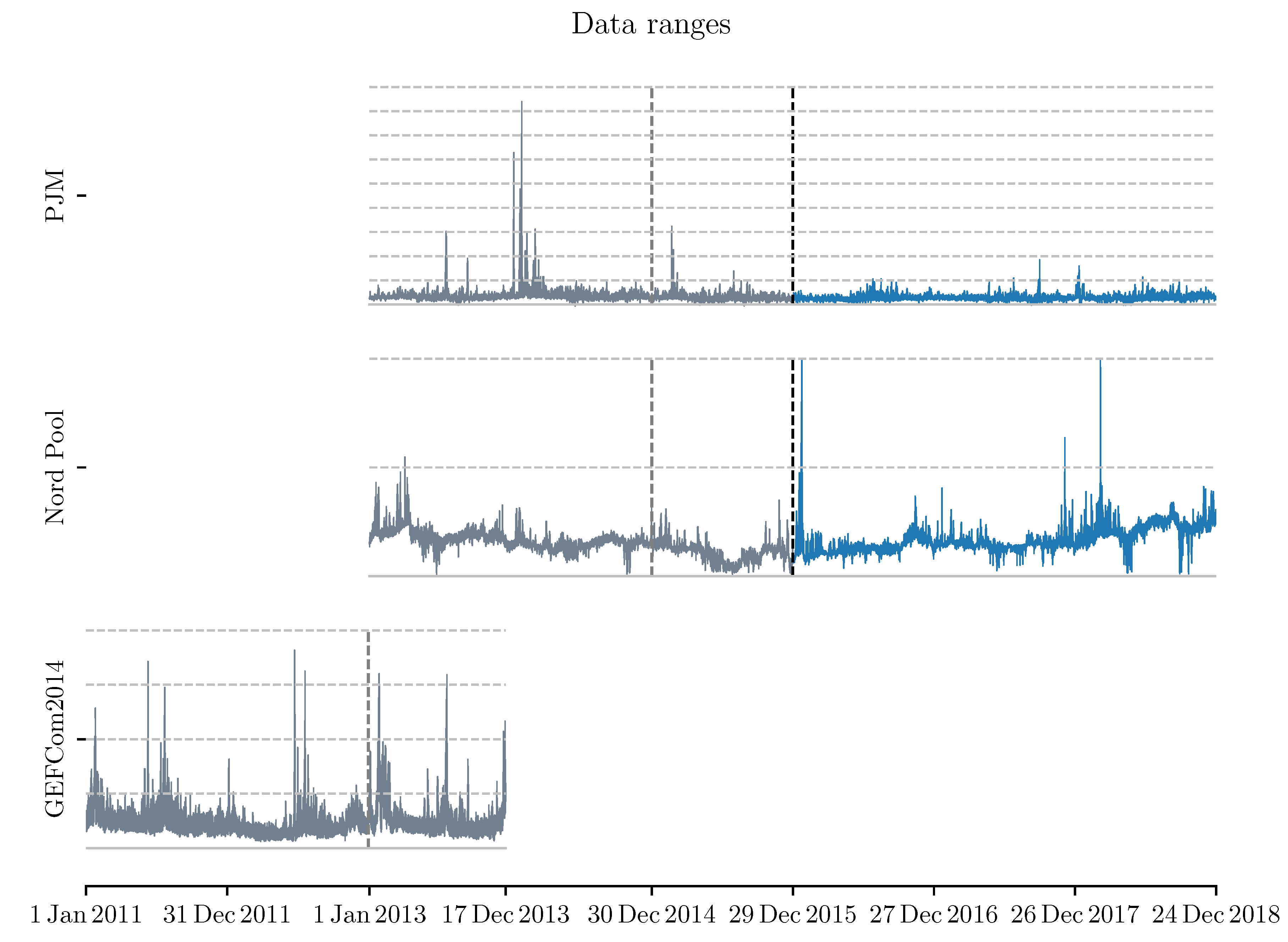
The timeline of data used in the study is presented in Figure 1, where the dashed vertical lines mark the ends of the longest initial calibration windows: Gray for the precalibration phase and black for the main testing. Horizontal grid lines indicate the price levels: The solid one, i.e., the lowest, corresponds to 0 and all lines (dashed, solid) are separated by 100 units (USD/MWh for PJM and GEFCom2014, and EUR/MWh for Nord Pool). The three series exhibit very distinct characteristics. The PJM data noted a long period of pronounced price spikes in the beginning of 2014 (reaching over 500–800 USD/MWh) and nearly no prominent spikes in the test years (2016–2018). The Nord Pool, on the other hand, shows an increased variability over time, along with price spikes to both high and low prices (albeit not reaching the negative values). The reason for such a changing behavior lies, most probably, in the changes in the generation mix and usage patterns. The six year-long history shows that the markets are not stagnant, and the modeling should be performed on the recent data. The third, shorter series (GEFCom2014) is only used to infer the hyper-parameters on, and does not demonstrate a change in the characteristics similar to the other two series.
For each of the data series, an exogenous series of the day-ahead load forecasts is also available. To simplify the notation, the letter p is used to refer to the prices, letter z to refer to the exogenous data and letter x—to present a transformation that is applied identically to both prices and load forecasts, i.e., . The notation also makes use of capital letters, subscripts and superscripts to indicate the step of the data preprocessing.
3.2. Hyper-Parameter Choice
The procedure of training a neural network (i.e., the process of fitting the weights to the connections present in the structure) and the topology of the network itself is defined by a collection of hyper-parameters. Firstly, the user can choose from different network-related options, such as the structure (neurons, layers, connections between them, activation functions). Secondly, the choice expands to various parameters that describe the training (e.g., the optimization algorithm, the loss function, training time, sampling, etc.). Note, that there are options that depend on the optimization algorithm, such as the learning rate. However, their impact on the forecasting performance is not covered in this study.
Naturally, the parameters come with predefined default values, which are typically an effect of limited empirical tests by the authors, or are theoretically derived based on the characteristics of the underlying processes. The defaults, albeit being “reasonable”, might turn out to be sub-optimal for a specific task. To address this issue, one can resort to some form of hyper-parameter optimization. This can be addressed in multiple ways, each of them having its own strengths and weaknesses. One of the methods—the one used in this study—requires the user to perform an additional numerical experiment to test values from a predefined hyper-parameter grid, using different data than the main out-of-sample test period. The advantage of such an approach are small requirements for information about the impact of each parameter on the forecasting performance, a mere specification of possible values suffices. Moreover, after performing the additional experiment, the method does not impose additional computational burden; the approach presented here implicitly assumes that the best parameter sets remain unchanged over time. On the other hand, the hyper-parameter precalibration procedure is very resource-consuming and any unnecessary value of a parameter inserted into the grid results in significantly increased computational burden. The method is, however, well suited for explanatory analysis, as it can help to understand the impact of each parameter on the final outcome and thus to create better forecasting models in the future. Additionally, a grid search mitigates one major shortcoming of step-by-step optimization techniques: It lessens the impact of the noise on the model chosen. Step-by-step optimization procedures applied on such volatile data are prone to end up in a suboptimal point of the parameter space due to the randomness of the error evolution over consecutive trial runs.
3.3. Calibration Window Length
The length of the calibration window used for fitting models—both statistical and neural network based—is a very important, but overlooked issue. In a recent series of papers [21,22,23], researchers aim to find combinations of calibration windows that yield the best forecasts and a scheme to aggregate the information contained within. A thorough examination of the impact of the calibration window length on the forecasting accuracy is out of scope of this study. However, motivated by the results, we will use three calibration window lengths: 364, 728 and 1092 days. Note, that the shortest window length we use (364 days) is much longer than the 28- or 56-day windows used in the previous studies. This is a consequence of using richer, multi-parameter input structures.
3.4. Forecast Averaging
Forecast averaging across different calibration window lengths is only one of the possibilities, but can be applied to all of the models used in the study. Another option can be introduced by generating multiple forecasts using different parameters, such as the parameter in least absolute shrinkage and selection operator (LASSO) or the hyper-parameter sets for neural networks. The former, however, was not used in this study. Based on a limited numerical experiment, the forecasting performance depends on the parameter in a close-to-convex way, which would require either taking poor forecasts into the ensemble, or taking forecasts very similar to each other. For neural network models, especially with a full parameter grid search, one should be able to simply take the top N performing parameter sets and create an ensemble out of them. The top entries obtained this way would present a variety of different parameter combinations, and additionally limiting the negative impact of local optimization and random initialization on the forecast robustness. This leads to the next ensembling possibility, namely averaging consecutive runs of an identically parametrized model [3]. This technique, however, is not utilized in this study, as (i) it requires n times more computational effort for n runs and (ii) further averaging the forecasts averaged over different parameter sets would result in diminishing returns. Naturally, the potential of averaging forecasts does not end here. It is possible to combine forecasts obtained using different models, different estimation techniques, etc. However, the two methods used in this study, namely averaging forecasts of one model, obtained using different calibration window lengths and considering top-performing hyper-parameter sets, are straight-forward to implement. Moreover, the former has already been shown to be effective in EPF, whereas the latter is a natural choice for the hyper-parameter grid search performed in this study.
3.5. Variance Stabilizing Transformations
Electricity price time series are characterized by pronounced spikes. Having such spiky data, using one of the so-called variance stabilizing sransformations (VSTs) is a well-known technique to obtain more accurate predictions [24,25,26].
In this study the data series were normalized prior to applying the VST, and the normalization process was as follows. First, we compute the median value of the series X (i.e., for the prices and for the load forecast) in whole calibration window, then we derive the median absolute deviation (MAD) around the median and adjust it by a factor for asymptotically normal consistency to the standard deviation, i.e., , where is the 75th percentile of the standard normal distribution. The normalized price has the form
and the normalized load forecast is obtained analogously. Having the normalized series, one can apply the chosen transformation: , where or .
The VST used in the study is the arc hyperbolic sine (asinh), which is straightforward to implement, symmetric around zero and its inverse—the hyperbolic sine—is also computationally efficient, thus making it feasible for use in electricity price forecasting [26,27,28]. The asinh transformation is defined as follows:
After computing the forecasts for the transformed prices, an inverse transformation is applied to obtain the price predictions in terms of normalized prices: . Next, to compute the final predictions in correct units, one has to invert the normalization procedure: . Note, that only the price series is forecasted in the process. The variance stabilizing transformation, however, is applied independently for both series, i.e., the medians and MADs are computed separately for the prices and loads.
3.6. Early Stopping Condition for Neural Networks
The neural network training process is typically interrupted before the algorithm converges. This is done to avoid over-fitting the network’s weights to the presented data and to ensure that the network can accurately infer based on the unseen data [29]. However, the use of early stopping leads to two issues. Firstly, the data has to be split into training and validation samples, leaving less data to train the model on. Secondly, the procedure induces additional hyper-parameters to be determined: A ratio of training to validation data, the method of splitting the series (block, random or a mixture of the two) and the so-called “patience”, i.e., a parameter that fixes the number of iterations without validation score improvement after which the training is stopped.
Instead, the study uses a fixed number of iterations (called epochs), and the value is chosen empirically as the best-performing in the precalibration phase. Not only such an approach simplifies the study setup, but also serves as a medium to find an optimal training length. Additionally, the model is trained using all of the available data.
3.7. Software
LASSO models were estimated using the scikit-learn [30] library for Python. The neural network models were trained using Python programming language and Keras library (version 2.2.4) [31] with either Theano or TensorFlow backend (both yielded results with negligible differences in the limited comparison performed). All neural networks were invoked with default floating point precision (float32).
4. Datasets
4.1. Modeling Settings
The study can be divided into two parts: Precalibration phase that involves a hyper-parameter grid search, and testing phase in which the tested hyper-parameter sets are used. However, there are several design decisions that were not a part of the hyper-parameter grid:
- VST used for both phases,
- calibration window length within the precalibration phase,
- transferring the hyper-parameter optimization results from one dataset to another.
To assess the need for VSTs when using neural networks, we have performed two repetitions of each experiment, one with the VST (asinh, see Section 3.5) applied, and one without. However, we did not allow to mix the approaches between the phases, meaning that for each precalibration dataset, we have obtained two separate sets of top models. In the testing part of the study, for VST-transformed data we have used only the parameter sets appointed using the VST, and similarly for the non-transformed data.
Lastly, we have included a dataset that does not contain an out-of-sample test set. This was done to check whether it is important to precalibrate on the data from the same market. To evaluate the potential differences between the hyper-parameter “origin”, for both of the test datasets, we had three best hyper-parameter sets: The one chosen for the GEFCom2014 data precalibration period, the one chosen for NP data, and the one chosen for PJM data.
Both phases used a rolling calibration window scheme (i.e., a calibration window of fixed length, directly preceding the forecasted day). For example, when forecasting the first day of the out-of-sample test period (i.e., 29 December 2015) with a 1092 day long calibration window, the model is trained on data from 1 January 2013 to 28 December 2015. After that, the calibration window is rolled by one day (2 January 2013–29 December 2015) to model the next day, 30 December 2015, etc.
4.2. Precalibration and Out-Of-Sample Testing Data
The precalibration procedure, i.e., the process of empirically finding the best hyper-parameter set for given test conditions (data origin, VST, see Section 3.2, Section 3.3 and Section 3.5) was performed on three data series. Two of them originate from electricity markets operating in the United States: The data used in GEFCom2014 competition [20] and the Pennsylvania-New Jersey-Maryland (PJM) Interconnection data, the third one is from the Scandinavian electricity exchange (Nord Pool, NP). Each of the data series used for precalibration comprises roughly three years (1092 day long subset for NP and PJM, 1082 days for GEFCom) of hourly data: Marginal prices as well as day-ahead load forecasts. It is worth noting, that these datasets present a distinct overview of liquid and well-established electricity markets. The diversity of generation sources and usage patterns is important for this study, as in the chapters to follow the patterns and dependencies discovered for one dataset will be to some extent used for other markets via the precalibrated hyper-parameters.
The second phase of the procedure uses the best precalibrated parameter sets to make predictions for either a completely different dataset (e.g., GEFCom → NP) or from the same market, but a different period (e.g., PJM 2013–2015 → PJM 2016–2018). The methodology implicitly assumes that the price response to the input variables (i.e., previous prices and exogenous series) does not vary throughout the years nor between the markets. This limitation is partially weakened by the rolling calibration window scheme used in the study.
The testing is performed on two datasets. In both cases the out-of-sample test period consists of 1092 days directly after the end of the data frame used for precalibration. Thus, the hyper-parameter optimization is done ex-ante from the forecasting point of view. Moreover, the performance of models based on different datasets is evaluated as well. On the other hand, models do not mix the VST used in the precalibration and the main evaluation periods (meaning that hyper-parameter sets obtained using asinh transformation will only be used in the asinh-transformed test setting). For each of the four test (dataset, VST) settings: (PJM, ID), (PJM, asinh), (NP, ID), (NP, asinh), three possible hyper-parameter collections can be derived: From PJM, NP and GEFCom data.
The longest initial calibration window (1092 days from 01.01.2013 until 28.12.2015) coincides with the data used for hyper-parameter precalibration. The data from 29.12.2015 onwards (next 1092 days, up until 24.12.2018) is used to evaluate the forecasts. Exogenous series for both datasets are visually very similar across the whole range, whereas the behavior of price series varies slightly with time. For the PJM data, the volatility of price series decreases in the test period. On the other hand, an adverse effect can be observed for the Nord Pool market.
5. Methodology
5.1. Benchmark Models
The predictive performance of the proposed approach is compared to a selection of different benchmarks: From the parsimonious ARX model, through parameter-rich LASSO structure to the DNN identical to the one used in the proposed approach, but using the default parameter set. This ensures a comprehensive assessment of not only the potential gains from using the neural networks themselves, but also the gains imposed by the precalibration approach. The latter is especially important given the computational cost of the precalibration procedure.
5.1.1. The Arx Expert Model
The first benchmark is a parsimonious autoregressive structure with exogenous variables (ARX), widely used in EPF. The model was originally proposed by [32] and later adopted by many researchers [28,33,34]. It is referred to as an expert model [35,36] due to the fact that it uses regressors that are derived either by empirical testing or knowledge of experts. The model uses a multivariate setting, which means that for each day, 24 separate models are trained, one corresponding to each hour of the day. It is important to note that such a setting limits the information contained in the model, as no information about hours different than the forecasted is included (apart from the minimum price). Within the model, the price for hour h of day d is modeled via the following formula:
where is the minimum of the previous day’s 24 hourly prices. It serves as both the link with all yesterday’s prices and a correction factor for the base price level. The variable is the load forecast for hour h (see Section 4). Lastly, the three weekday dummies correspond to Saturday, Sunday and Monday, respectively. They allow to better model the intraweek seasonality by describing the different price levels for Saturdays, Sundays and Mondays, when the dependence of prices on the prices from the day before is different than for the rest of the weekdays.
Given the ARX structure (1), the linear responses of price to the regressors are then estimated using ordinary least squares (OLS) on a fixed-length sample of past observations (i.e., the calibration window). The optimal length of the calibration window is strongly dependent on several factors, including the model used, the dataset, the forecasted period and the data transformation. To mitigate the inability of choosing the optimal calibration window ex-ante this study resorts to using three calibration window lengths, corresponding to roughly a year, two years and three years. This approach allows for an improved performance and stability of the forecasts, while also limiting the computational burden, particularly the computations required to find the best performing calibration window lengths.
5.1.2. Lasso-Derived Parameter-Rich Model
The second benchmark can be seen as a natural enrichment of the ARX structure, as it does not add any regressor of different origin. It rather presents the information regarding all 24 h of the day among the regressors, instead of only selecting data corresponding to the forecasted hour. In theory, it should improve the predictions by adding very similar neighboring hours, as well as including better peak and off-peak base levels. Because of a greatly increased number of regressors (100 instead of 8), a different model estimation method is used, namely the least absolute shrinkage and selection operator (LASSO, originally proposed by [37]), as it limits the number of explanatory variables included in the model by selecting only the most relevant ones. Moreover, the process of regularization is automatic and requires the user to choose only the regularization parameter , which can be empirically fitted for the specific data through Cross Validation [38]. Such an approach was used in this study, with 100 values of the parameter tested via 10-fold CV trials. LASSO-estimated parameter-rich models are widely used in EPF literature [28,35,36,39].
The baseline model estimated via the LASSO is simply an augmented version of Equation (1). It models the price for hour h of day d via the formula:
where indicates the lowest price of yesterday, similarly as in Equation (1). Note, that in this case, the minimum is always included in the model twice (as opposed to the ARX model, where double inclusion takes place only once per 24 trained models). However, it does not create linearly dependent columns (the lowest price is observed in different hours of the day), and has an independent parameter estimated. By analogy, the variables correspond to weekday dummies for Saturday, Sunday and Monday, whereas is the forecasted load for i-th hour of day d.
It is important to note, that albeit having exactly the same structure and inputs, the model is fitted separately for each hour of the day (i.e., we use a multivariate framework, see Section 5.1.1), and by extension, the regularization and selection take place for each hour independently. This allows to define the model in an universal way, which can be seen as the largest available parameter space, yet still allows to properly derive 24 potentially different models—each specifically tailored for a single hour.
5.1.3. The Default Dnn Benchmark
The last benchmark was constructed with a two-way comparison in mind. Firstly, it is used to compare the non-linear structure with the linear data description of the LASSO. The second comparison, however, is even more interesting, as it allows to measure the gains from using the computationally expensive two-step approach.
The benchmark assumes the use of all default hyper-parameter values (see Section 3.2). Unfortunately, there are two exceptions, without which the model would produce completely unusable forecasts. First of them is the epochs parameter that governs the maximum number of full iterations of the algorithm over the training set. The default value of a single epoch is not suitable in our case, therefore to provide a benchmark that is able to achieve reasonable results, the epochs value was set to 500. The value was chosen as the most popular entry among the best-performing models in the precalibration phase, which also means that most of the precalibrated DNN models are trained for 500 epochs. There was no early stopping condition, meaning that each calibration of a neural network consisted of exactly 500 iterations over the full training dataset.
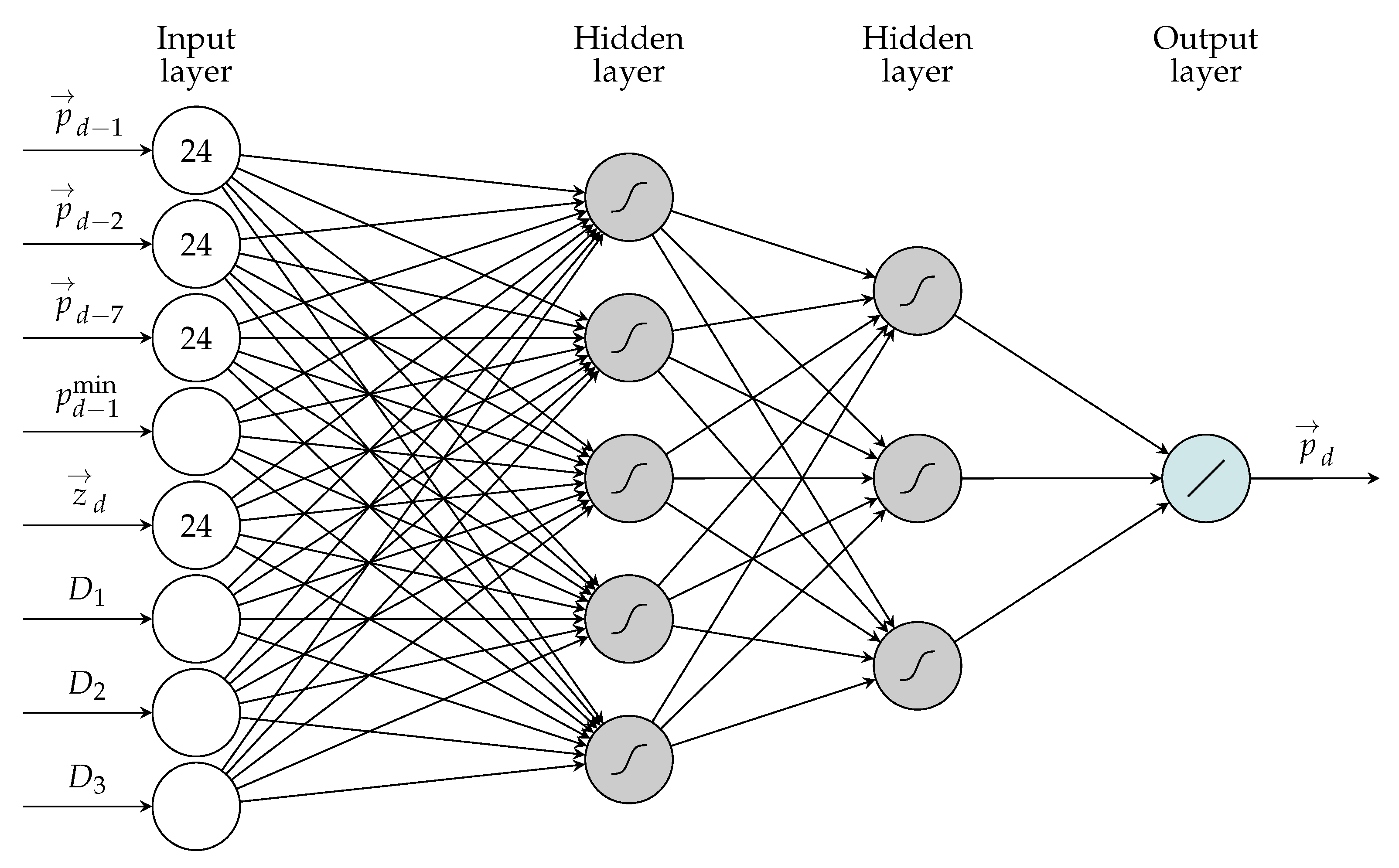
All neural network models use exactly the same information as in Equation (2), however, in an multi-output (vectorized, similarly to vector autoreggresion) framework with all 24 h of the day modeled at once. This is done due to the significant computational burden of model estimation. Modeling the whole 24-hour vector at once, but resorting to only one model trained per day of forecast, requires only about of the CPU time when compared to the framework with 24 independent models, each predicting a single hour of the day (i.e., a typical framework used by ARX and LASSO benchmarks). Moreover, the nonlinear, dense structure of a network should in theory allow to minimize the potentially negative impact of such a setting, which has been shown to occur for some datasets [28]. Therefore, the DNN model can be visualized as shown in Figure 2.
As mentioned, the benchmark uses default hyper-parameter values in the Keras library. More precisely, the network structure of choice was a densely connected network with 100 input neurons, two hidden layers with 100 neurons each and 24 output neurons, the training length was fixed at 500 epochs of ADAM stochastic gradient descent-based optimizer with MAE loss function and a batch_size of 32. The validation_split parameter was set to 0 (i.e., there was only training set) and activation functions were set to sigmoid and linear, respectively for both hidden layers and for the output layer. See Section 5.3 for descriptions of the hyper-parameters.
The second exception from the default values was the activation function. When not specified explicitly, Keras always uses the linear activation (more specifically, the identity function). This results in a fully linear model, and does not perform well for EPF. To address that, all of the implemented activation functions were tested in this setting. The sigmoid activation scored well (despite being slightly outperformed by very similar hard-sigmoid in some cases), and was chosen as the ex-post best performer for the DNN default benchmark.
5.2. Fine-Tuned Neural Network Model
This DNN model uses exactly the same network structure and inputs as the DNN benchmark (see Section 5.1.3), but differs in terms of the hyper-parameters (see Section 3.2 and Section 5.3). The main idea behind the two-step fine-tuning proposed in this study is to automatically evaluate hyper-parameter sets and use the best 5 of them to compute the final forecasts (the number 5 was chosen via an additional numerical experiment, using more yields diminishing returns, while increasing the computational time). The resulting forecasts are later averaged (creating an ensemble) across both the hyper-parameter sets and calibration window lengths. The aggregation process is described in Section 5.4. As the ensemble smoothens the random noise of the respective forecasts and generally performs better than the input forecasts, it is treated as the final output model of the approach.
5.3. Training Parameters Grid Search
The first stage of the approach involves forecasting the validation dataset using a wide range of hyper-parameter sets. To avoid making any assumptions, the parameter space is formed as a full grid of 1008 possible combinations of four parameters. There are two categorical options, namely the optimization algorithm and the activation function of all hidden neurons (which was identical for both hidden layers of deep networks). Secondly, two numerical (integer) parameters were included.
The first one—the batch size—governs the number of training samples presented at once to the optimizer. This translates to the number of samples after which the weights in the network are updated. The second numerical parameter controls the maximum epoch count. An epoch during training corresponds to one full iteration over all training samples. The maximum value of this parameter was chosen to be very high for this problem, while still maintaining the computational time on a rational level. Further increasing of this value would most likely result in overfitting. In conjunction with the batch size, it controls the frequency and the total count of weight updates in the network. It is important to note, that only fixed epoch counts are used in the study, i.e., the training in every case consisted of the specified iterations over the dataset and no early stopping condition was implemented. This is a possible point of future improvement, however, this approach—at a cost of a larger hyper-parameter space—provides an empirically validated combination of parameters, see Section 3.6 for discussion.
The specific values tested during the precalibration procedure were as follows:
- Seven optimization algorithms based on the stochastic gradient descent: Adam, Adamax, Adagrad, Adadelta, Nadam, SGD, RMSprop.
- Four activations: eLU, ReLU, tanh, sigmoid, same activation function was used for every hidden neurons, and the output layer was always linear.
- Four values of max epochs: 50, 100, 200, 500.
- Eight values of the batch size: 16, 32, 64, 96, 128, 192, 256, 384, 768.
As a result, for each of the (Data, VST) tuples, the list of hyper-parameters with corresponding errors is obtained. The errors are computed based on the forecast using a rolling calibration window of model and a specific parameter set. Note, that the considered hyper-parameter space is not exhaustive and did not cover e.g., the network depth or width, which were fixed.
5.4. Parameter Choice and Forecast Aggregation
After performing the parameter space grid search described in Section 5.3, the parameter sets are ranked according to the mean absolute error. Then, for each of the (Data, VST) tuples, the five sets yielding the lowest MAE are selected. The final forecasts use an ensemble of forecasts obtained using all five derived parameter sets, see Section 3.4. Note, that this kind of averaging (i.e., averaging outcomes of forecasts with different hyper-parameters) is applicable only to neural networks in the two-step approach.
However—as discussed in Section 3.3—there is a potential for improvements in forecast accuracy by using multiple models with an identical structure, but obtained using different calibration window lengths. As argued by [21], there are some window length combinations that yield robust gains, but the testing was not conducted for parameter-rich neural networks. Nevertheless, to optimize the outcomes and benefit from the technique to a limited extent, all models and benchmarks are evaluated using three lengths of calibration windows. The results are presented for each of them separately and as an ensemble of forecasts. The lengths: 52, 104 and 156 weeks, which corresponds to roughly 1, 2 and 3 years were chosen ad-hoc. This also applies to the forecasts obtained using the two-step approach; for each of the top five parameter sets, three forecasts are computed and additionally an ensemble over calibration windows is derived. Moreover, the ensemble across different parameter sets is created for each calibration window length as well as an ensemble consisting of 15 individual forecast runs.
6. Results
The section presents the obtained results and discusses the differences between the methods. The structure is as follows. Firstly, the results of the hyper-parameter space search are described with the analysis of the most often picked values. Secondly, the predictive accuracy of benchmark models is summarized. Next, the results of the fine-tuned DNNs are presented, and the importance of the precalibration dataset is investigated. Lastly, the computational feasibility is studied, with the assessment of the computational complexity of both the fine-tuned DNNs and the benchmark models.
6.1. Preliminary Hyper-Parameter Space Search
This section contains a brief discussion on the diversity of the top parameter sets across different precalibration conditions, as well as the most common occurrences of some of the parameter values. However, it is important to note that while there are some patterns, they might be solely caused by the random nature of the network training methods and might not be applicable to other (even similar) forecasting tasks. The precalibration procedure itself does not rely on those patterns and is in principle invariant to aforementioned randomness.
The first—and potentially the most important—observation regards the activation function used in the hidden layers. Among the precalibration parameter set results sigmoid was present most often (23 of 30 times), with 5 tanh and 2 exponential linear unit (eLU) entries. Interestingly, rectified linear unit (ReLU) activation did not appear even once among the top results, in spite of its popularity in the literature [5,6].
The second observation concerns the network training iterations over the dataset. Most commonly picked parameter sets were trained for 500 epochs. Only seven out of 30 best-performing parameter sets contained shorter (200 epochs) training.
As far as the optimizer is concerned, there was no unanimity. The ADAM, ADAMAX and ADAGRAD optimizers were chosen most commonly, however, every optimizer aside from stochastic gradient descent (SGD) occurred at least once in all 30 top picks.
6.2. Benchmark Models
Each of the benchmark models was computed for three calibration window lengths of 364, 728 and 1092 days and tested on all 1092 days of the out-of-sample test window. Additionally, an ensemble of these three forecasts was derived (by taking an arithmetic mean of the forecasts for each hour). The results in terms of MAE are presented in Table 1. It is important to note how well the default DNN benchmark preforms in all of the cases, being on par with or outperforming the second-best LASSO.
6.3. Fine-Tuned and Aggregated Forecasts
Each of the benchmark models was computed for three calibration window lengths of 364, 728 and 1092 days and tested on all 1092 days of the out-of-sample test window. Additionally, an ensemble of these three forecasts was derived (by taking an arithmetic mean of the forecasts for each hour). The results in terms of MAE are presented in Table 1. It is important to note how well the default DNN benchmark preforms in all of the cases, being on par with or outperforming the second-best LASSO.
This section presents the results obtained using deep neural networks with hyper-parameters chosen via the precalibration procedure. The non-transformed data (i.e., with ID VST) and asinh-transformed data are treated separately. It is important to note, that due to the small differences between the hyper-parameter sets obtained using different datasets, presented here are the average error metrics of three ensembles, each based on different precalibration dataset.
Aggregate relative metrics comparing the fine-tuned ensembles with both DNN default and LASSO ensembles are presented in Table 2.
6.3.1. Models Calibrated to Raw Data
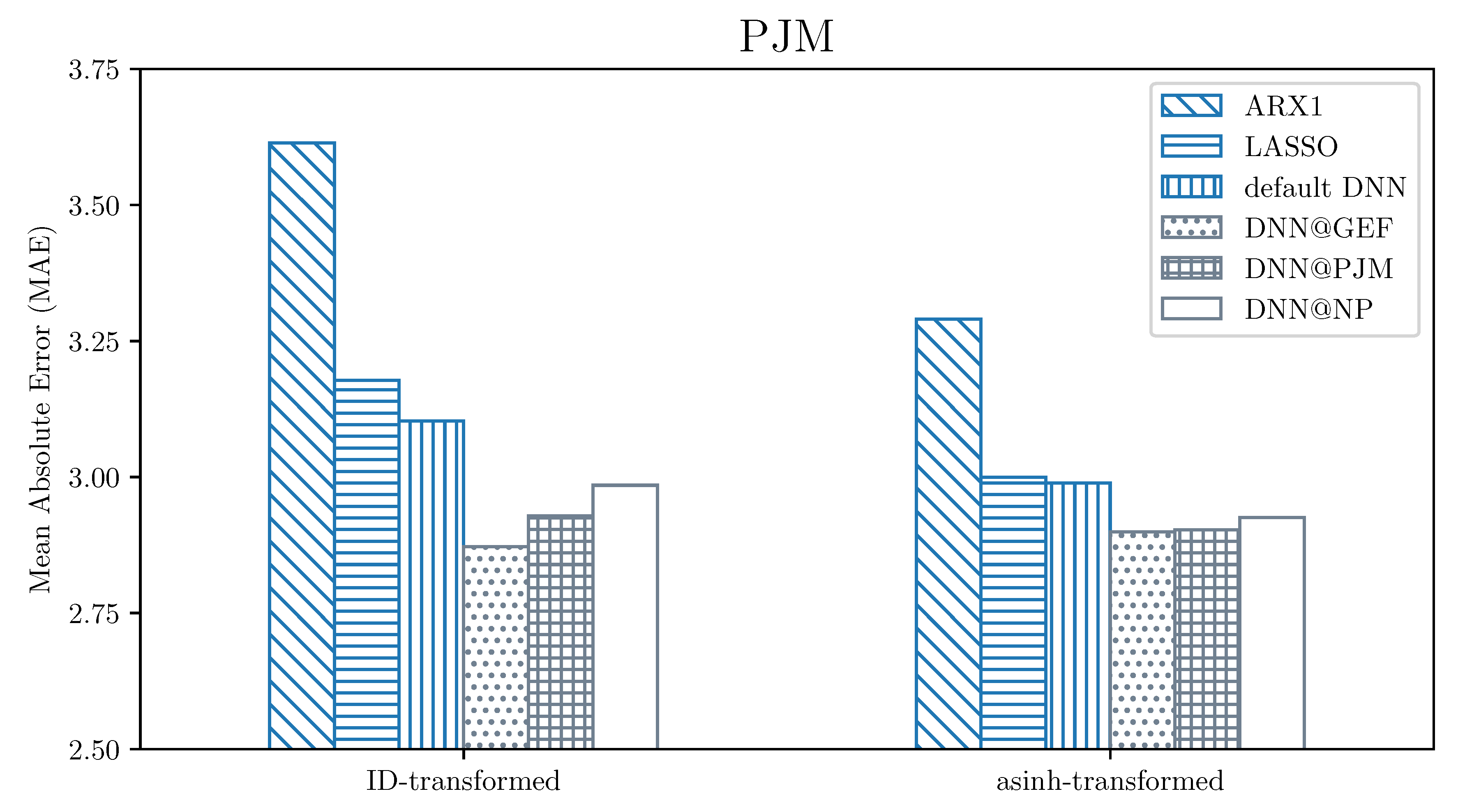
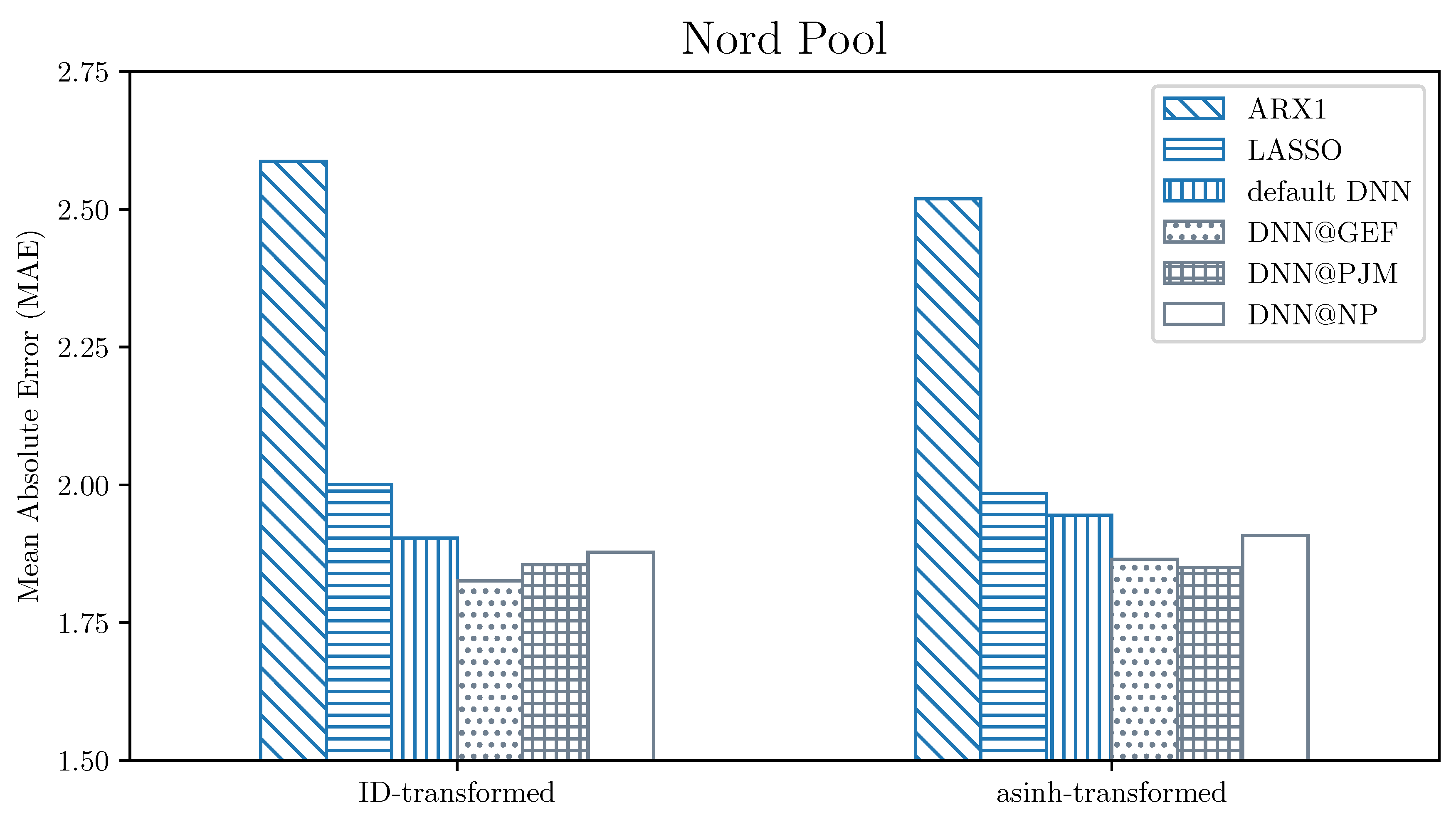
When considering models calibrated to raw data, for PJM dataset some of the individual (non-aggregated) networks were able to outperform the best benchmark (the DNN default benchmark, which is an ensemble itself) that scored , whereas final ensemble of tuned DNNs—. The situation changes slightly for Nord Pool data, where ensembling is needed to outperform the best benchmark (also DNN default, with score of )—no single model does so. However, the final forecast of the fine-tuned DNN model—namely the ensemble across both the top parameter sets and different calibration window lengths—scores significantly lower (). The difference is even larger when we consider the second best benchmark: The ensemble of 3 LASSO forecasts. Such a benchmark yielded MAEs of and , respectively for PJM and Nord Pool, which makes the obtained DNN results even more significant and shows the shortcomings of using linear models on data as volatile as observed in electricity markets.
One can also conclude that averaging across different calibration window lengths yields very robust estimates, especially for PJM data. It is important to note that for PJM data, individual models trained using the 3 year long calibration window are underperforming when compared to shorter windows. This is mainly due to the period of extremely high volatility at the beginning of 2014. Using the 3 year long calibration window includes this information in the model for over a third of the out-of-sample test period. The impact of these outliers can be seen clearly for all three benchmarks. On the other hand, the forecasts chosen via the precalibration procedure are not such strongly penalized, which shows the potential of this methodology.
6.3.2. Models Calibrated to Asinh-Transformed Data
The overall outcome is very similar for the asinh-transformed data; after applying the VST, the fine-tuned DNN forecasts are also able to outperform the best benchmark. What is interesting to note, is that the 3 year long calibration window is no longer underperforming for the PJM dataset. Even more so, it performs on par or better than the shorter ones. The same observation can be made for the benchmarks (besides the default DNN benchmark, but that is most likely due to randomness), including the DNN default. The final ensemble scores were equal , and , respectively for fine-tuned DNNs, DNN default and LASSO ensembles.
The Nord Pool data exhibit a situation where none of the single forecasts are able to outperform the best benchmark. The ensembles across calibration window lengths or hyper-parameter sets are mostly able to match the best benchmark score with little improvement. In this case, however, the gain from using all 15 forecasts instead of 3 (ensemble across calibration window lengths) or 5 (across top parameter sets) is very substantial, and the final forecast scores MAE of , which significantly outperforms both the DNN default () and LASSO ensembles ().
Overall, the improvement imposed by the VST was negligible for ensemble forecasts: For Nord Pool data there was even a (slight) performance degradation, for both DNN default benchmark and the optimized networks. When the effects of applying the VST on linear structures (ARX, LASSO) are considered, this implies that the non-linear representation of a neural network is able to effectively model the strongly non-linear relations found in the data without resorting to any external techniques. This makes the neural networks a very universal modeling tool, as it removes the need of choosing the right VST for the data (the asinh function used in this study is only one of many possible functions, see [26] for a comparison performed using linear models).
6.4. Importance of the Precalibration Dataset for the Fine-Tuned Forecast
As can be seen in Figure 3 and Figure 4, the fine-tuned neural network ensembles outperform significantly all of the benchmarks. Interestingly, the performance differences between different datasets of origin of the hyper-parameters are not strongly pronounced, with GEFCom data (dotted bars) being slightly better than the two other datasets. This result may seem counter-intuitive (it should be better to use the same origin of data for both the hyper-parameter selection and the testing), however the GEFCom data window for used for the precalibration serves well as an “exemplary” EPF dataset, with uniformly distributed spikes and without visible structural changes throughout.
These examples show that the hyper-parameters sets can successfully be found using data of different origin (but describing the same phenomenon), and that the GEFCom dataset is slightly better than the remaining two datasets that we have considered. However, regardless of the choice, the results show that an ex-ante hyper-parameter selection resulting in accurate forecasts is possible.
6.5. Computational Feasibility of Proposed Solutions
To assess the computational feasibility of the neural network methods, timed runs were performed on a machine equipped with an Intel Core i5-3570 CPU. Additionally, benchmark generation times are included for reference (ARX1 and LASSO). All listed times refer to the generation of price forecasts for one day (extracted from a longer sample to reduce the initialization overhead). The times listed for DNN models reflect the worst-case scenario over all of the hyper-parameter sets. Generation times for final forecasts (i.e., an ensemble over three or 15 runs) are reported, and hyper-parameter optimization step is not considered here—it is assumed that an initial computational effort can be computed over a long period of time or on a multi-node computer cluster, and there is no need to rerun the optimization in the day-to-day operation. The results overview is presented in Table 3.
The parsimonious structure of ARX model and an exact solution obtained via matrix operations allow for generation of an ensemble forecast for the next day in approximately 15 milliseconds, with negligible dependence on the VST. Both the LASSO benchmark and DNN model are orders of magnitude slower to obtain, due to the iterative estimation. LASSO, despite being a simple linear model, utilizes cross validation, which greatly increases the times needed to compute forecasts; it takes and s respectively for the ID-transformed and asinh-transformed data, with the difference coming most probably from the faster convergence.
Assessing the times for the DNN model is not straightforwards, hence, a worst-case scenario is presented. Specifically, we assume that for every calibration window length we take the longest time across all hyper-parameter sets as the time needed to generate a single forecast, which is then multiplied by 5 (ensemble across hyper-parameter sets). This results in the longest runtimes, 116 and 121 s respectively for ID and asinh transformations. The time does not vary much between them due to the fixed number of iterations over the dataset.
To sum up, the DNN model, even in the worst-case scenario is computationally feasible, i.e., the result can be obtained in near real-time on a contemporary hardware. The LASSO model can be accelerated significantly by either limiting the cross validation space for the regularization parameter or by using a fixed parameter (or a parameter based on information criteria) instead.
7. Conclusions
Obtaining the accurate day-ahead electricity price forecasts is crucial for any entity that heavily bases the profitability on the electricity prices, e.g., a power generating company. The accurate forecasts can greatly benefit the decision-making process in such a utility and can lead to better (in terms of the financial outcome) decisions being made. In the long run, availability of more accurate forecasts for the market participants can lead to lowering the price volatility, which in turn could result in e.g., lower risk of the long-term investments that are strongly dependent on the electricity prices. Another use of the more accurate price forecasts lies in the growing field of demand response and its role in the transformation of the electricity markets [40,41].
The deep neural network used in the study allows, along with the hyper-parameter optimization and ensembling scheme, for a significant outperformance of statistical-based approaches. This kind of modeling provides the user with a set of very well-performing and feature-rich tools, which—as shown by the default DNN benchmark—works relatively well with little tuning. However, the tuning itself is no longer an option, but rather a necessity, as using pure defaults would yield a 1-epoch trained network with the linear activation function in the hidden layers. The largest performance penalty would obviously come from training limited to 1 epoch, however, the activation function itself also plays a major role in achieving a well-rounded model.
The two-step approach—as proposed here—proves to be a very robust technique, with excellent performance across almost all of the test scenarios and can be applied in practice. It does, however, come at a price. The generation of the precalibration forecasts alone is a serious computational difficulty. On the other hand, the approach uses many independent forecasts (in this case, 1008 for each dataset, VST pair), which makes it feasible to run in parallel on high-performance computer clusters or using cloud computing. With that in mind, the precalibration procedure does not need to be reapplied (often). This study assumed that the precalibration procedure would not be repeated for the whole three year long test period. Moreover, if the precalibration was to be updated periodically (e.g., every three months) it would be much faster because only incremental updates of the forecasts are needed, which would not be straightforward to implement using step-by-step hyper-parameter optimization.
The main takeaway from this study is that the hyper-parameters can be automatically tailored to fit a specific task, and the selection can be performed ex-ante. Such forecasts consistently outperform even the DNN benchmark used in the study. Looking at the results from a different perspective, all of the neural network-based models were much better-performing than the LASSO model estimated using the same information. The performance gain is best visible on the non-transformed PJM data, which exhibits a change in the volatility of the price series. Non-linear layers enable the model to effectively cope with the data that proves difficult to forecast using linear models.
The research, however, does not conclude the idea of using a neural network precalibrated using a hyper-parameter grid search fully. While a well-performing application is presented, there are still interesting aspects left for future research, such as the network topology (deep or shallow, dense or sparse?) or the periodic hyper-parameter recalibration.
Funding
This work was partially supported by the Ministry of Science and Higher Education (MNiSW, Poland) through grant No. 0219/DIA/2019/48. Calculations have been carried out using resources provided by the Wrocław Center for Networking and Supercomputing (WCSS; http://wcss.pl) under grant no. 466.
Conflicts of Interest
The author declares no conflict of interest.
References
- Huisman, R.; Huurman, C.; Mahieu, R. Hourly electricity prices in day-ahead markets. Energy Econ. 2007, 29, 240–248. [Google Scholar] [CrossRef] [Green Version]
- Cruz, A.; Muñoz, A.; Zamora, J.L.; Espínola, R. The effect of wind generation and weekday on Spanish electricity spot price forecasting. Electr. Power Syst. Res. 2011, 81, 1924–1935. [Google Scholar] [CrossRef]
- Marcjasz, G.; Uniejewski, B.; Weron, R. On the importance of the long-term seasonal component in day-ahead electricity price forecasting with NARX neural networks. Int. J. Forecast. 2019, 35, 1520–1532. [Google Scholar] [CrossRef]
- Lago, J.; De Ridder, F.; Vrancx, P.; De Schutter, B. Forecasting day-ahead electricity prices in Europe: The importance of considering market integration. Appl. Energy 2018, 211, 890–903. [Google Scholar] [CrossRef]
- Lago, J.; Ridder, F.D.; Schutter, B.D. Forecasting spot electricity prices: Deep learning approaches and empirical comparison of traditional algorithms. Appl. Energy 2018, 221, 386–405. [Google Scholar] [CrossRef]
- Chinnathambi, R.A.; Plathottam, S.J.; Hossen, T.; Nair, A.S.; Ranganathan, P. Deep Neural Networks (DNN) for Day-Ahead Electricity Price Markets. In Proceedings of the 2018 IEEE Electrical Power and Energy Conference (EPEC), Toronto, ON, Canada, 10–11 October 2018; pp. 1–6. [Google Scholar]
- Schnürch, S.; Wagner, A. Machine Learning on EPEX Order Books: Insights and Forecasts. arXiv 2019, arXiv:1906.06248. [Google Scholar]
- Zhang, J.; Tan, Z.; Wei, Y. An adaptive hybrid model for short term electricity price forecasting. Appl. Energy 2020, 258, 114087. [Google Scholar] [CrossRef]
- Gareta, R.; Romeo, L.M.; Gil, A. Forecasting of electricity prices with neural networks. Energy Convers. Manag. 2006, 47, 1770–1778. [Google Scholar] [CrossRef]
- Kuo, P.H.; Huang, C.J. An Electricity Price Forecasting Model by Hybrid Structured Deep Neural Networks. Sustainability 2018, 10, 1280. [Google Scholar] [CrossRef] [Green Version]
- Xie, X.; Xu, W.; Tan, H. The Day-Ahead Electricity Price Forecasting Based on Stacked CNN and LSTM. In Intelligence Science and Big Data Engineering; Peng, Y., Yu, K., Lu, J., Jiang, X., Eds.; Springer International Publishing: Cham, Switzerland, 2018; pp. 216–230. [Google Scholar]
- Zahid, M.; Ahmed, F.; Javaid, N.; Abbasi, R.A.; Zainab Kazmi, H.S.; Javaid, A.; Bilal, M.; Akbar, M.; Ilahi, M. Electricity Price and Load Forecasting using Enhanced Convolutional Neural Network and Enhanced Support Vector Regression in Smart Grids. Electronics 2019, 8, 122. [Google Scholar] [CrossRef] [Green Version]
- Yang, W.; Wang, J.; Niu, T.; Du, P. A novel system for multi-step electricity price forecasting for electricity market management. Appl. Soft Comput. 2020, 88, 106029. [Google Scholar] [CrossRef]
- Yang, Z.; Ce, L.; Lian, L. Electricity price forecasting by a hybrid model, combining wavelet transform, ARMA and kernel-based extreme learning machine methods. Appl. Energy 2017, 190, 291–305. [Google Scholar] [CrossRef]
- Kath, C.; Ziel, F. The value of forecasts: Quantifying the economic gains of accurate quarter-hourly electricity price forecasts. Energy Econ. 2018, 76, 411–423. [Google Scholar] [CrossRef] [Green Version]
- Paraschiv, F.; Erni, D.; Pietsch, R. The impact of renewable energies on EEX day-ahead electricity prices. Energy Policy 2014, 73, 196–210. [Google Scholar] [CrossRef] [Green Version]
- Díaz, G.; Coto, J.; Gómez-Aleixandre, J. Prediction and explanation of the formation of the Spanish day-ahead electricity price through machine learning regression. Appl. Energy 2019, 239, 610–625. [Google Scholar] [CrossRef]
- Keles, D.; Scelle, J.; Paraschiv, F.; Fichtner, W. Extended forecast methods for day-ahead electricity spot prices applying artificial neural networks. Appl. Energy 2016, 162, 218–230. [Google Scholar] [CrossRef]
- Halužan, M.; Verbič, M.; Zorić, J. Performance of alternative electricity price forecasting methods: Findings from the Greek and Hungarian power exchanges. Appl. Energy 2020, 277, 115599. [Google Scholar] [CrossRef]
- Hong, T.; Pinson, P.; Fan, S.; Zareipour, H.; Troccoli, A.; Hyndman, R.J. Probabilistic energy forecasting: Global Energy Forecasting Competition 2014 and beyond. Int. J. Forecast. 2016, 32, 896–913. [Google Scholar] [CrossRef] [Green Version]
- Hubicka, K.; Marcjasz, G.; Weron, R. A Note on Averaging Day-Ahead Electricity Price Forecasts Across Calibration Windows. IEEE Trans. Sustain. Energy 2019, 10, 321–323. [Google Scholar] [CrossRef]
- Marcjasz, G.; Serafin, T.; Weron, R. Selection of Calibration Windows for Day-Ahead Electricity Price Forecasting. Energies 2018, 11, 2364. [Google Scholar] [CrossRef] [Green Version]
- Serafin, T.; Uniejewski, B.; Weron, R. Averaging Predictive Distributions Across Calibration Windows for Day-Ahead Electricity Price Forecasting. Energies 2019, 12, 2561. [Google Scholar] [CrossRef] [Green Version]
- Janczura, J.; Trück, S.; Weron, R.; Wolff, R. Identifying spikes and seasonal components in electricity spot price data: A guide to robust modeling. Energy Econ. 2013, 38, 96–110. [Google Scholar] [CrossRef] [Green Version]
- Diaz, G.; Planas, E. A Note on the Normalization of Spanish Electricity Spot Prices. IEEE Trans. Power Syst. 2016, 31, 2499–2500. [Google Scholar]
- Uniejewski, B.; Weron, R.; Ziel, F. Variance Stabilizing Transformations for Electricity Spot Price Forecasting. IEEE Trans. Power Syst. 2018, 33, 2219–2229. [Google Scholar] [CrossRef] [Green Version]
- Schneider, S. Power spot price models with negative prices. J. Energy Mark. 2011, 4, 77–102. [Google Scholar] [CrossRef] [Green Version]
- Ziel, F.; Weron, R. Day-ahead electricity price forecasting with high-dimensional structures: Univariate vs. multivariate modeling frameworks. Energy Econ. 2018, 70, 396–420. [Google Scholar] [CrossRef] [Green Version]
- Geman, S.; Bienenstock, E.; Doursat, R. Neural Networks and the Bias/Variance Dilemma. Neural Comput. 1992, 4, 1–58. [Google Scholar] [CrossRef]
- Pedregosa, F.; Varoquaux, G.; Gramfort, A.; Michel, V.; Thirion, B.; Grisel, O.; Blondel, M.; Prettenhofer, P.; Weiss, R.; Dubourg, V.; et al. Scikit-learn: Machine Learning in Python. J. Mach. Learn. Res. 2011, 12, 2825–2830. [Google Scholar]
- Chollet, F. Keras. 2015. Available online: https://keras.io (accessed on 4 September 2020).
- Misiorek, A.; Trück, S.; Weron, R. Point and interval forecasting of spot electricity prices: Linear vs. non-linear time series models. Stud. Nonlinear Dyn. Econom. 2006, 10, 2. [Google Scholar] [CrossRef] [Green Version]
- Gaillard, P.; Goude, Y.; Nedellec, R. Additive models and robust aggregation for GEFCom2014 probabilistic electric load and electricity price forecasting. Int. J. Forecast. 2016, 32, 1038–1050. [Google Scholar] [CrossRef]
- Weron, R.; Misiorek, A. Forecasting spot electricity prices: A comparison of parametric and semiparametric time series models. Int. J. Forecast. 2008, 24, 744–763. [Google Scholar] [CrossRef] [Green Version]
- Uniejewski, B.; Nowotarski, J.; Weron, R. Automated Variable Selection and Shrinkage for Day-Ahead Electricity Price Forecasting. Energies 2016, 9, 621. [Google Scholar] [CrossRef] [Green Version]
- Ziel, F. Forecasting Electricity Spot Prices Using LASSO: On Capturing the Autoregressive Intraday Structure. IEEE Trans. Power Syst. 2016, 31, 4977–4987. [Google Scholar]
- Tibshirani, R. Regression shrinkage and selection via the lasso. J. R. Stat. Soc. B 1996, 58, 267–288. [Google Scholar] [CrossRef]
- Hastie, T.; Tibshirani, R.; Friedman, J. The Elements of Statistical Learning: Data Mining, Inference, and Prediction; Springer Series in Statistics; Springer: New York, NY, USA, 2009; Chapter 7. [Google Scholar]
- Marcjasz, G.; Uniejewski, B.; Weron, R. Beating the Naïve—Combining LASSO with Naïve Intraday Electricity Price Forecasts. Energies 2020, 13, 1667. [Google Scholar] [CrossRef] [Green Version]
- O’Connell, N.; Pinson, P.; Madsen, H.; O’Malley, M. Benefits and challenges of electrical demand response: A critical review. Renew. Sustain. Energy Rev. 2014, 39, 686–699. [Google Scholar] [CrossRef]
- Larsen, E.M.; Pinson, P.; Leimgruber, F.; Judex, F. Demand response evaluation and forecasting—Methods and results from the EcoGrid EU experiment. Sustain. Energy Grids Netw. 2017, 10, 75–83. [Google Scholar] [CrossRef]
Figure 1.
Timeline of the datasets considered in the study. The periods used for hyper-parameter calibration are drawn in gray, whereas the out-of-sample test periods are in blue.
Figure 1.
Timeline of the datasets considered in the study. The periods used for hyper-parameter calibration are drawn in gray, whereas the out-of-sample test periods are in blue.

Figure 2.
Visualization of the Deep Neural Network (DNN) structure, used in both the DNN benchmark and the main DNN models (hidden layer sizes are not reflected here; the net used in the study comprised 100 neurons in each hidden layer). The arrows over symbols correspond to 24 separate input/output neurons, with a dense connection structure.

Figure 3.
Visualization of the MAE errors for PJM data across the benchmark (darker shade) and fine-tuned (lighter shade) ensembles, separately for identity (ID) (left part) and asinh-transformed data (right part). Each bar represents the ensemble of all forecasts made using a given model (represented by a filling pattern). The @DATA notation refers to the precalibration dataset used for hyper-parameter selection.

Figure 4.
Visualization of the MAE errors for Nord Pool data across the benchmark (darker shade) and fine-tuned (lighter shade) ensembles, separately for ID (left part) and asinh-transformed data (right part). Each bar represents the ensemble of all forecasts made using a given model (represented by a filling pattern). The @DATA notation refers to the precalibration dataset used for hyper-parameter selection.


Table 1.
Mean absolute errors for the benchmarks. The lowest score for each of the VSTs and datasets is marked in bold.
Table 1.
Mean absolute errors for the benchmarks. The lowest score for each of the VSTs and datasets is marked in bold.
| ID-Transformed Data | ||||||||
| Benchmark | PJM | Nord Pool | ||||||
| 364 | 728 | 1092 | ensemble | 364 | 728 | 1092 | ensemble | |
| ARX1 | 3.476 | 3.581 | 4.128 | 3.614 | 2.690 | 2.608 | 2.563 | 2.587 |
| LASSO | 3.239 | 3.280 | 3.632 | 3.178 | 2.125 | 2.044 | 2.020 | 2.001 |
| DNN default | 3.183 | 3.241 | 3.970 | 3.103 | 2.018 | 2.060 | 2.043 | 1.903 |
| Asinh-Transformed Data | ||||||||
| Benchmark | PJM | Nord Pool | ||||||
| 364 | 728 | 1092 | ensemble | 364 | 728 | 1092 | ensemble | |
| ARX1 | 3.303 | 3.305 | 3.350 | 3.290 | 2.536 | 2.574 | 2.537 | 2.519 |
| LASSO | 3.076 | 3.047 | 3.054 | 3.000 | 2.048 | 2.039 | 2.009 | 1.984 |
| DNN default | 3.158 | 3.156 | 3.230 | 2.989 | 2.033 | 2.115 | 2.087 | 1.945 |
Table 2.
Relative improvements in MAE when using the fine-tuned DNN ensemble instead of the benchmark models.
Table 2.
Relative improvements in MAE when using the fine-tuned DNN ensemble instead of the benchmark models.
| Fine-Tuned DNN vs. | Dataset | ID | Asinh |
|---|---|---|---|
| LASSO benchmark | Nord Pool | ||
| PJM | |||
| default DNN benchmark | Nord Pool | ||
| PJM |
Table 3.
Approximate times needed to generate one day of the forecasts using different methods. Note the differences in the units. The time listed for the DNN is a worst-case scenario, see the description in the text.
Table 3.
Approximate times needed to generate one day of the forecasts using different methods. Note the differences in the units. The time listed for the DNN is a worst-case scenario, see the description in the text.
| ARX | LASSO | Fine-Tuned DNN | |
|---|---|---|---|
| time | ca. 15 ms | 30–40 s | below 120 s |
© 2020 by the author. Licensee MDPI, Basel, Switzerland. This article is an open access article distributed under the terms and conditions of the Creative Commons Attribution (CC BY) license (http://creativecommons.org/licenses/by/4.0/).
Share and Cite
MDPI and ACS Style
Marcjasz, G. Forecasting Electricity Prices Using Deep Neural Networks: A Robust Hyper-Parameter Selection Scheme. Energies 2020, 13, 4605. https://0-doi-org.brum.beds.ac.uk/10.3390/en13184605
AMA Style
Marcjasz G. Forecasting Electricity Prices Using Deep Neural Networks: A Robust Hyper-Parameter Selection Scheme. Energies. 2020; 13(18):4605. https://0-doi-org.brum.beds.ac.uk/10.3390/en13184605
Chicago/Turabian StyleMarcjasz, Grzegorz. 2020. "Forecasting Electricity Prices Using Deep Neural Networks: A Robust Hyper-Parameter Selection Scheme" Energies 13, no. 18: 4605. https://0-doi-org.brum.beds.ac.uk/10.3390/en13184605
Note that from the first issue of 2016, this journal uses article numbers instead of page numbers. See further details here.