A Long-Term Condition Monitoring and Performance Assessment of Grid Connected PV Power Plant with High Power Sizing Factor under Partial Shading Conditions

Abstract

Partial shading conditions of photovoltaic (PV) modules often occurs in urban areas leading to losses in electricity power generation of the PV power plant. The purpose of this study is to present how the PV power plant with high value of inverter power sizing factor (K_inv) can achieve high performance and power production under partial shading conditions with high shading losses. In this paper the results of long-term monitoring, performance analysis and experimental results are presented, while the results are compared to the estimated values calculated using PVsyst software. The study focused on the PV power plant at the Faculty of Technical Sciences (FTS) in Novi Sad, Republic of Serbia, for the period between the years 2012 and 2019. It has been shown that the values of PV power plant performance parameters are better than expected (very high), and resemble the power plants operating without shading. The high value of the inverter power sizing factor may lead to occasional saturation of the inverter when certain conditions are met, but most of the times it allows the inverter to operate at a more optimal power level. PV module soiling and power degradation is within the limits mentioned in the literature. The increase in K_inv in the partial shading conditions favorably affects the performance, does not degrade the efficiency of the inverter at saturation, reduces the effect of soiling and aging of PV modules, leading to higher power production.

1. Introduction

The beginning of 21st century is characterized by a significant increase in the amount of energy generated from renewable energy sources. Further increase in the generation from these types of energy is imperative for achieving the sustainable development goals (SDGs) formulated by the United Nations and contain 14 goals, with seven directly tied with affordable and clean energy (SDG 7). The most important achievement offered by the SDG 7 should be the reduction of harmful gasses emission and the development of sustainable industry [1]. A significant contribution to achieving SDG 7 in developing countries are hybrid renewable energy microgrids [2]. Renewable energy sources, in particular electrical energy sources, can significantly benefit the proposed cause, justifying the numerous studies aiming to improve their performance [3]. Currently, the most important renewable energy sources are hydro, wind and solar energy. Developed countries have the highest installed capacities of renewable energy sources (RES), followed by several developing countries. The most important countries where the RES energy utilization is crucial are Iceland, Sweden, USA, China and India [4].

The fastest increase in installed RES capacity in the world corresponds to PV power plants. The countries with the highest installed PV capacity are China, Japan, Germany, the United States, Italy, United Kingdom, India, France, Australia and Spain. The cumulative installed capacity worldwide in 2019 has reached the 580.16 GW mark, with the annual energy generation of 720 TWh [5]. The estimates show that the new solar PV installed capacity forecast is at 105 GW in 2020 [6]. It is projected that by 2030 the total installed capacity will be 2.84 TW [7]. The majority of the PV systems are utility scale PV power plants, however distributed PV power plants make up about 40% of the total installed capacity and should not be disregarded. In the Republic of Serbia, the beginning of the most recent century saw the legislations and decrees have been passed that better support the integration of RES in the Serbian power system. However, currently the maximum installed capacity that could receive the feed-in tariff is limited to only 10 MW of total installed power (for PV power plants in the Republic of Serbia). From 2011 to 2015, there were 9 MW of installed power in PV power plants that applied for the incentive (5.4 MW in ground PV systems, 2 MW in roof-top less than 30 kW and 1.5 MW in roof-top 30 kW to 500 kW). In the presented period, the total annual installed capacities were as follows: 20 kW, 250 kW, 2306 kW, 5391 kW and 798 kW [8]. After this period, the interest in PV power plants decreased significantly, since no increase in the total limit for feed-in has not been increased. From the year 2020, some changes are expected, such as introduction of net metering for distributed and auctions for utility PV power plants. In comparison to the most European countries, Republic of Serbia has a very good solar potential. The only European countries with higher potential are southern European countries such as: Portugal, Spain, Italy, Greece, etc. The total global irradiance for Serbia at the horizontal plane is between 1200 kWh/m² and 1500 kWh/m². For the optimally inclined surfaces the values can range from 1300 kWh/m² in the north to 1700 kWh/m² in the south [9].

Improvements can be noticed almost daily in every area of RES technology. Due to new materials and improved manufacturing technology the power, efficiency and robustness is constantly improving for wind generators, PV modules and inverters [4]. In the last several years, significant advancements have been made in the characteristics of monocrystalline and polycrystalline PV modules. Currently several advanced technologies are available on the market such as passivated emitter rear contact cells (PERCs), tunnel oxide passivated contact cells (TOPcons), half-cut cells, 1/3 cells technology, bifacial PV cells, N-type cell technology, dual-glass technology, multi-busbar technology, high-density encapsulation technology, etc. These type of cell technologies and their various combinations have led to enhanced performances of PV modules, especially in regards to power, power losses due to aging, temperature coefficient, efficiency, potential induced degradation (PID), light induced degradation (LID), shading effect, robustness and other. These parameters are very important since they lead to increased installed power and generation per square meter of surface, resulting in further decreases in harmful gas emissions.

Research papers presenting analyses of grid-connected PV system performance usually describe low power, residential and commercial systems with installed powers of up to 200 kW. In most cases, these are roof-top PV plants located in highly dense urban areas, with frequent operation under partial shading conditions is typical. The literature usually does not consider the influence of partial shading conditions and inverter power sizing factor on the PV power plant operation. It is a well-known fact that partial shading conditions can significantly decrease the system performance, i.e., significantly decrease the energy production. Additionally, the inverter power sizing factor can influence the performance, operating conditions, energy production, return of investment and levelized cost of electricity [10].

Table 1. The PV power plants analyzed by the literature.

Reference/Country	Beginning of Work	Pinv (kW)	Kinv	Shading Condition	Analysis Period (Years)
[11] Spain	1997	2	0.91	not stated	1
[12] Poland	2000	1.2	0.83	possible	3
[13] Crete	2002	2.5	1.15	not stated	1
[14] Algeria	2006	1.6	1.00	not stated	1
[15] Spain	2008	100	0.99	not stated	1
		100	1.01
[16] Ireland	2008	1.7	1.01	not stated	1
[17] Egypt	2010	3.8	0.95	not stated	1
[18] Serbia	2012	2	1.00	not stated	1
[19] Sardinia	−	12.5	1.05	not stated	1
		300	1.07
[20] India	−	11.2	1.02	no	1
[21] Thailand	−	3 × 2.2	0.74	not stated	5 day
[22] India	−	190	0.97	not stated	3
[23] Nepal	−	4 × 30	0.96	possible	1
[24] Malaysia	−	2 × 3	1.23	possible	3/4
This paper Serbia	2011	8	1.20	yes	8

presents references that have analyzed PV power plant performance sorted by the chronology of the development, [11,12,13,14,15,16,17,18,19,20,21,22,23,24]. Table 1 presents the year when the operation began, inverter power (P_inv), K_inv, shading conditions, and the analysis period. As observed from the table, most analyses had been performed for one year. In contrast, this paper will present an analysis of system operation during an 8-year period.

By observing the value of the K_inv, it is evident that the oldest PV power plants have values that are less than one (0.8–0.9), which was acceptable according to the available knowledge at the time. Other papers have K_inv values around one, even if according to [25] this value can go up to 1.25 for optimally inclined PV modules. Apart from the PV plant in Sardinia, where the K_inv approaches 1.1 (1.07), only two other PV power plants have a factor larger than 1.1 (Crete—1.15 and Malaysia—1.23).

This paper analysis the performance of the PV power plant with high inverter power sizing factor (K_inv = 1.2) under partial shading conditions due to local surrounding buildings. The analysis period covers the operation from the start-up to the end of the year 2019, i.e., 8 years of operation. As noted, the most specific feature of the PV power plant is the high value of K_inv, which was very uncharacteristic at the time of the construction (in 2011).

2. Location and PV Power Plant Description

The PV power plant is installed at the University of Novi Sad campus, at the Faculty of Technical Sciences (FTS). This power plant was the first in Vojvodina, the autonomous province of the Republic of Serbia, to acquire the permission to be connected to the distribution system (DS). Considering just the technical aspect, the selected location is less than optimal, since there are two high buildings in the near vicinity from the east side (educational building—15 m and FTS tower—23 m) shading the PV modules. The Figure 1 shows the PV module micro-location on the flat roof.

In regard to the unfavorable micro-location, prior to the installation, the most suited part of the roof and PV module inclination was selected using PVsyst software (PVsyst SA, Satigny, Switzerland), in order to maximize the energy generation. PV modules are facing south with the inclination of 30°. Using the sun path diagram, acquired from PVsyst, the total shading losses are estimated at 8.2%.

The main system components are PV modules, inverter, switching equipment, protective equipment and monitoring system. A STP8000TL-10 (SMA Solar Tehnology AG, Niestetal, Germany) inverter with two maximum power point tracking (MPPT) inputs has the rated power of 8 kW. At every MPPT input there is one connected array of 20 PV modules, where each module (JKM240P-60, Jinko Solar, Shanghai, China) has the rated power of 240 Wp. The total installed power of the PV modules is 9.6 kWp, making the inverter power sizing factor 1.2. The PV power plant has a Sunny Sensorbox (SMA Solar Tehnology AG, Niestetal, Germany) meteorological data station, with a calibrated solar irradiation sensor for in-plane irradiance measurement and PT100 sensors for measurement of ambient and PV module temperatures. Sunny Sensorbox is connected to the power plant monitoring system Sunny Webbox (SMA Solar Tehnology AG, Niestetal, Germany) that collects the values of ambient conditions, input and output values of the inverter.

3. PV Module and Partial Shading Model

The model of the PV module begins with the single-diode model where photo generated currents I_PH, diode current I_d, parallel resistance current I_p and the module output current I are defined. Based on the Kirchhoff’s current law we can conclude the following [26,27]:

$$I_{PH}-I_d-I_p-I=0$$

(1)

When adequate equations are substituted in the Equation (1) for parallel resistance current and diode current, and the equation is rearranged to represent the PV module current, the following equation is true [27]:

$$I=I_{PH}-I_0·\left[exp\left(\frac{q·\left(V+I·R_s\right)}{{\gamma }_I·k·T}\right)-1\right]-\frac{V+I·R_s}{R_p}$$

(2)

where I₀ is the diode inverse saturation current, q = 1.602176 × 10⁻¹⁹ C is the charge value of an electron, V represents PV module voltage, R_S is the PV module series resistance, R_p stands for parallel resistance, γ_I is the ideality factor, k = 1.380648 × 10⁻²³ J/K is Boltzmann’s constant and T is the PV module temperature.

It has been shown in Ref. [27], that using Equation (2) it is possible to derive the PV module model dependent on the catalogue parameters (nameplate parameters). The equation to calculate PV module current based on the given parameters is presented in the following equation:

$$I=I_{SC}·\left[1-X·\left(exp\left(\frac{V}{Y·V_{OC}}\right)-1\right)\right]$$

(3)

where X and Y are functionally dependent on the following parameters of the PV modules I_M, V_M, I_SC and V_OC [27].

In order to model the influence of partial shading concept the theoretical background used in Ref. [28] can be used. If A and A_s define the PV module surface and sunny part of PV modules respectively, then the ratio of total and sunny surface of PV module can be defined as:

$$\frac{A_S}{A}=\frac{1+\frac{d}{b·\cos \beta }}{1+\frac{\tan \beta }{\tan \alpha }}$$

(4)

where d is the distance of the obstacle to the PV module, β is PV module inclination angle, α is the solar angle and b is the PV module length.

If 15-min values of solar irradiation G, total PV array surface At in respect to the shading factor η_S and efficiency of the PV module η_S is known, the production of the PV array can be expressed as [28]:

$$W_{ARY}={\displaystyle \sum }_i^{365}{\displaystyle \sum }_j^{np}0.25·A{t}_{ij}·G_{ij}·{\eta }_{PV}$$

(5)

where np is the number of 15 min periods in a day when inverter is operational and i is the ordinal number of the day in a year.

Using the Equations (4) and (5), as in [28], and by adjusting the values of the obstacle distance and PV modules to the respective case, the final equation for the energy calculation for PV power plant can be expressed as:

$$W_{ARY}={\displaystyle \sum }_i^{365}{\displaystyle \sum }_j^{np}\frac{0.25}{1000}·A·G_{ij}·{\eta }_{SYS}\left(T, SR\right)·r·\frac{1+\frac{d}{b·\cos \beta }}{1+\frac{\tan \beta }{\tan \alpha }}·{\eta }_S$$

(6)

where η_SYS dependent on the PV module temperature T and soiling ration SR, r is the number of PV arrays in the PV power plant and η_S is defined as in Ref. [28].

4. Analysis Methodology

In the following paragraphs the most important parameters of PV power plant that were measured or calculated within this paper will be presented. These parameters can be used for comparison of operational characteristics, verification of operation and the calculation of efficiency in PV power plants.

The inverter and PV array need to be matched according to the voltage, current and the power, which is done in the system planning phase, when the inverter power sizing factor is defined. The inverter power sizing factor K_inv that has significant influence on financial and technical parameters of the PV system is defined as:

$$K_{inv}=\frac{P_{ARYN}}{P_{INVAC}}$$

(7)

P_INVAC is the rated inverter output power, while P_ARYN is the total power of the PV array that is defined as rated power at the standard test conditions (STC), when the PV cell temperature is 25 °C, the irradiance is 1000 W/m² and air mass spectrum AM = 1.5. The value of the K_inv can be selected (projected) in the design phase of the PV power system, when several factors need to be considered such as: PV module position, ambient conditions at the location, inverter efficiency, electrical and non-electrical losses, etc. [29]. However, more often than not, this parameter is influence by the available surface for the PV modules installation and the wishes (usually cost cutting) of the investors, when the value of the K_inv can be lower than recommended.

The ideally expected PV array yield E_ARYID, at STC, can be calculated as a product of effective in-plane irradiation H_ARY, the surface of PV array S_ARY and the efficiency of the PV modules η_PV at STC as:

$$E_{ARYID}=H_{ARY}·S_{ARY}·{\eta }_{PV}$$

(8)

The real electrical energy production for the PV power plant will depend on many different factors, that can be included in the calculation as specific system parameters. The total yearly energy yield E_AC can be calculated as the sum of the product of system efficiency η_SYS and the ideally PV array yield for each day:

$$E_{AC}={\displaystyle \sum }_{i=1}^N{\eta }_{SYS,i}·E_{ARYID,i}$$

(9)

The final system yield Y_f represents the average generated electrical energy per PV array installed power. This value can be expressed as a daily, monthly or yearly value. The final system yield is calculated according to the following equation:

$$Y_f=\frac{E_{AC}}{P_{ARYN}} = {\displaystyle \sum }_i{P}_{AC,i}·{\tau }_i/P_{ARYn}$$

(10)

where τ_i is the i-th interval when the inverter output power P_ACi is measured or calculated. The denominator of Equation (4) is the rated PV array power and is considered to be constant for the PV system. Electrical energy generation of the PV system is variable during the year and has a very well-known tendency to drop from one year to another. Therefore, the value of the final system yield is constantly changing and also has a decreasing trend.

The reference yield Y_r is a ration between the total amount of the global solar irradiation at PV surface and the reference irradiance G_R:

$$Y_r=\frac{H_{ARY}}{G_R} = {\displaystyle \sum }_i{G}_i·{\tau }_i/G_R$$

(11)

The value Y_r can be considered as the equivalent number of h in the interval, during which the irradiance is equal to the reference, i.e., 1000 W/m². If the Y_r is expressed as [kWh/m²/day] then it has the following meaning—each incident kWh should ideally produce the array nominal power during one h. The reference yield is dependent on the meteorological conditions and the PV module configuration at the PV system location. Considering that Y_r is related to H_ARY that is measured at the PV power plant location, with the PV power plants that operate under partial shading conditions, the irradiation sensor position needs to be carefully considered.

According to the Standard IEC EN 61724 performance ratio PR for grid connected PV systems is defined as the ration between final system yield and reference yield [30]:

$$PR=\frac{Y_f}{Y_r} =\left({\displaystyle \sum }_i{P}_{AC,i}·{\tau }_i/P_{ARYn}\right)/\left({\displaystyle \sum }_i{G}_i·{\tau }_i/1000\mathrm{W}/{\mathrm{m}}^2\right)$$

(12)

The power of the PV array is defined at the STC and, in that regard, the PR can be considered as the ration between the generated electrical energy of the grid connected PV system and the ideal yield that would be achieved if the STC would apply constantly. The PR represents the value of the influence of all losses (light refraction losses, shading, soiling, aging, misalignment of components, PV conversion, wiring in the DC and AC subsystem, inverter efficiency and saturation) at the system output [13].

When analyzing PR in the time span shorter than one year, there can be a significant variation of the value. In this specific case, the temperature corrected performance ration factor (PR_T) is calculated. This factor assumes the correction of the PV array power as a function of the ambient temperature, consequently mitigating the influence of the seasonal variation of the PR.

The PR_T with the temperature correction for T_ref = 25 °C is calculated as:

$$P{R}_T =\left({\displaystyle \sum }_i{P}_{AC,i}·{\tau }_i/\left(1+\gamma ·\left(T_{PV,i}-25\right)\right)·P_{ARY}\right)/\left({\displaystyle \sum }_i{G}_i·{\tau }_i/1000\mathrm{W}/{\mathrm{m}}^2\right)$$

(13)

where γ is the temperature power coefficient for PV modules, T_PV is the actual temperature and T_ref is the referent temperature of PV modules. The average value of the PR_T is closer to 1 then standard PR [31,32].

The yearly capacity factor C_FYEAR presents the ratio of the yearly generated electrical energy and the yearly expected energy generation for 24 h operation under STC:

$$C{F}_{YEAR}=\frac{Y_f}{24·365}=\frac{E_{AC}}{P_{ARYN}·8760}$$

(14)

PV modules exposed to the influence of environmental conditions. One of the more significant influences comes from soiling at the surface of PV modules. Depending on the level of soiling, the power of the PV modules will drop, leading to the reduction of production. The value and the influence of the PV module soiling is defined with the soiling ratio (SR). SR is the ration of the power between the soiled PV module P_PVD and the clean PV module P_PVC [33]:

$$SR=\frac{P_{PVD}}{P_{PVC}}$$

(15)

During the exploitation, due to aging, the power of the PV modules also decreases. The module manufacturers declare the power reduction in the 25 year or 30-year period. The value of the power decrease during the PV system life-span operation can be described using degradation rate (DR), that is defined as follows:

$$DR=1-\frac{P_{PVT}}{P_{PVN}}$$

(16)

The power P_PVT is the PV module power at the STC in a defined measurement point during the PV module life-span (after a period of operation) and the P_PVN is the rated PV module power at the STC defined by the manufacturer [34].

5. The Results of Measurements

Following is the analysis of the eight-year measurement results for the PV power plant with the power of 8 kW that was officially commissioned on 25th of October 2011. The measurements, analyzed here are from the beginning of 2012 to the end of 2019. The calculated parameters, i.e., energy generation, Y_f, Y_r, PR and CF are calculated using logged data (Webbox and SensorBox) over the mentioned period with the data acquired once every 5 min. The irradiation sensor is a calibrated PV cell that can register irradiation between 0 W/m² and 1500 W/m² with the resolution of 1 W/m² and the accuracy of ±8%. The PT100 sensor is used for the air and PV module temperature measurement ranging between −20 °C and +110 °C, with the resolution of 0.1 °C and the accuracy of ±0.5%.

5.1. On Site Meteorological Conditions

It is a well-known fact that the most influential factors on PV power plant generation are irradiation and ambient temperature. In Novi Sad, where the respective power plant is located, the climate is moderate-continental with more and more often occurrences of extreme weather conditions.

During the previous operation these sever conditions occurred during two years. During the first year of operation (2012) the PV power plant felt the most severe weather conditions up to date. The yearly value of insolation hours was 2462 h, while the average value for the analyzed period was 2249 h. The winter of 2012 had the lowest air temperature ever with −28.7 °C, while the maximum air temperature was at the beginning of august with 39.9 °C [35]. The average monthly temperature for the analyzed period according to the data from the Republic Hydrometeorological Service of Serbia was 12.6 °C. The average monthly temperatures used by the PVsyst software are usually lower than the actual values, with yearly average at 12.2 °C. The average value of rainfall in the analyzed period was 672 L/m². In 2012 there was the least amount of rainfall, with the yearly average at 485 L/m², while the most rainfall happened during 2014 with the value of 816 L/m².

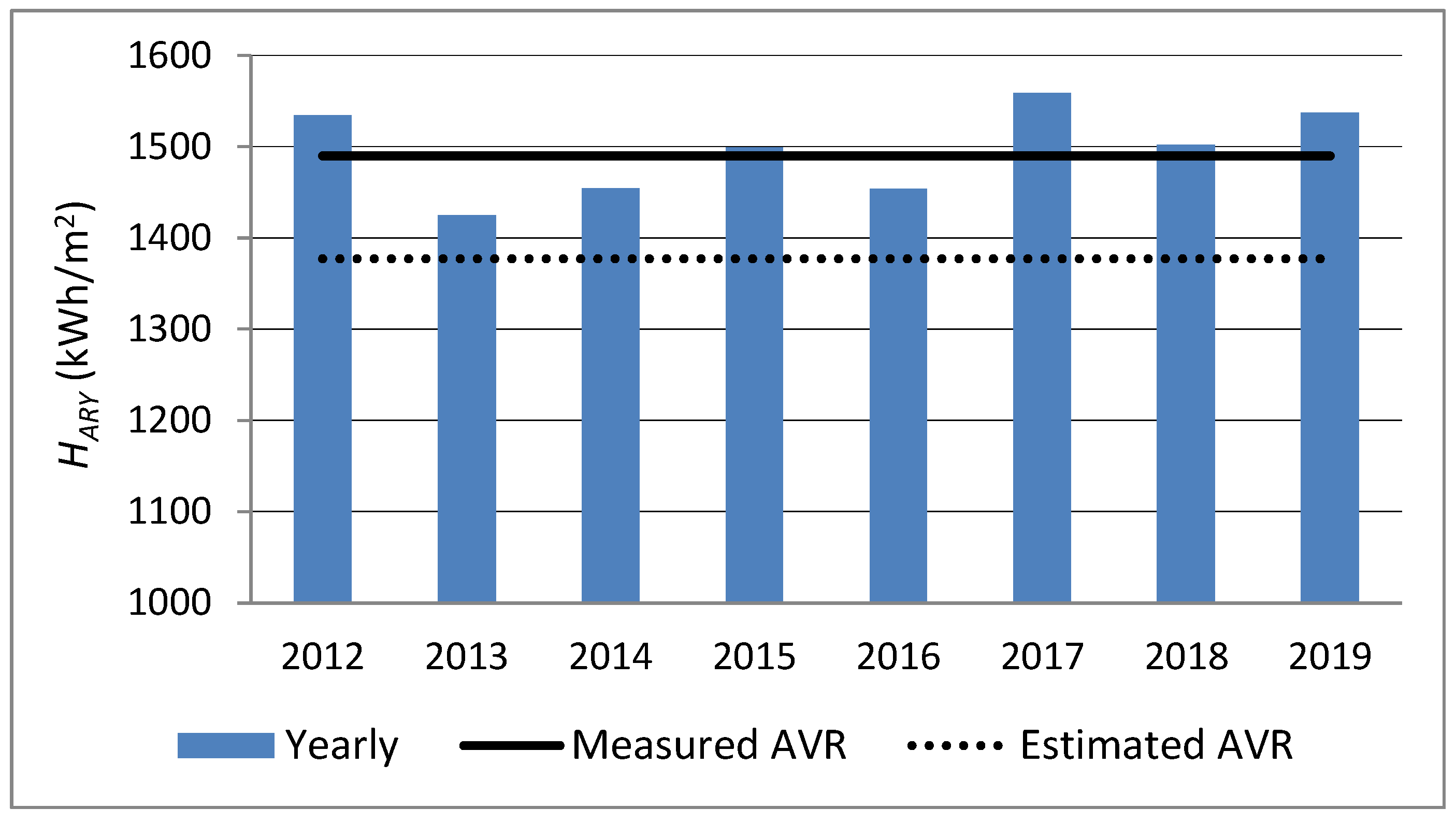
Figure 2 shows the sum of solar irradiation for every individual year in the respective period, acquired with the measurements from sensor box. The average value of the measured and the estimated solar irradiation at the PV array surface is 1490 kWh/m² and 1377 kWh/m² respectively. Measured values of irradiation are higher than the estimated for every year of the operation so far. Important thing to note is that the irradiation sensor position is chosen so that it is in the shade until all the modules exited the shade.

5.2. Estimated and Measured Performance

Using the PVsyst software, the ideal PV array yearly production is estimated according to Equation (8), considering that H = 1377 kWh/m²/year, the surface of 40 PV modules is S = 65 m² and the efficiency of the PV modules is 14.7%. The ideal PV array production calculated value is 13157 kWh annually. When all losses in the PV power plant are considered, the estimated energy to be supplied to the grid is 11,362 kWh annually. Energy generation, estimated using PVsyst software, when no shading is considered is 12,260 kWh, which is an increase of 7.9%.

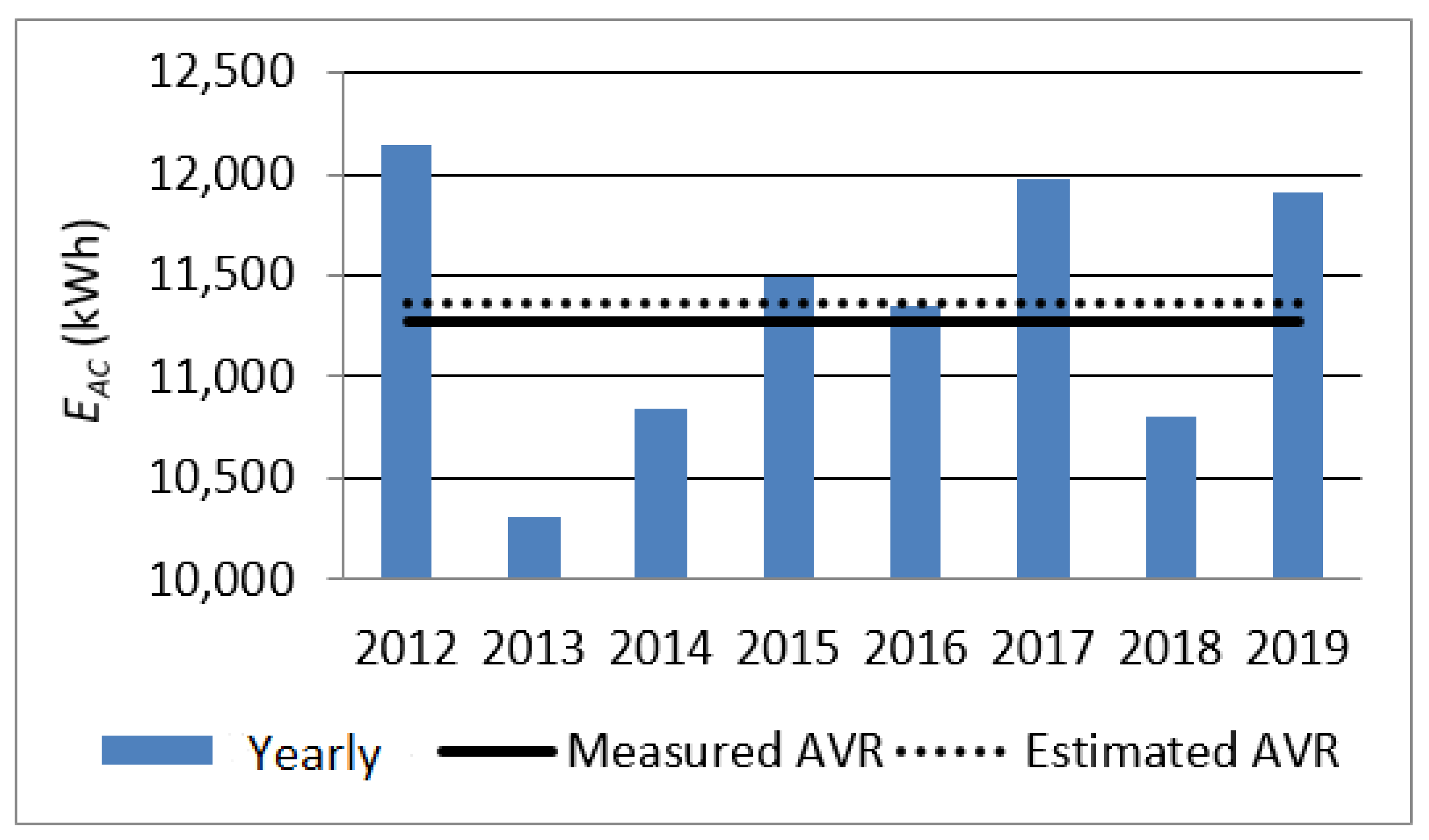
The generated energy from the data acquisition system is calculated using the measurement from the inverter integrated sensors. The generated electrical energy per year is presented in Figure 3. The same Figure shows the average yearly production at 11,275 kWh. This value is 0.78% lower than the estimated average production for the same period. It is easy to note that the highest production was during 2012, 2017 and 2019, when unusually high number of insolation hours occurred.

The PV power plant had no production for 21 days due to PV modules being covered by snow (the longest period was 7 days in February of 2012.) and due to system protection or supply outage for total of 34 days during the analyzed period of operation. It is estimated that the total loss of production is around 1000 kWh. The PV plant operation had never been down due to an element malfunction to this date. Total energy production during the 8 years of operation is 90.835 MWh.

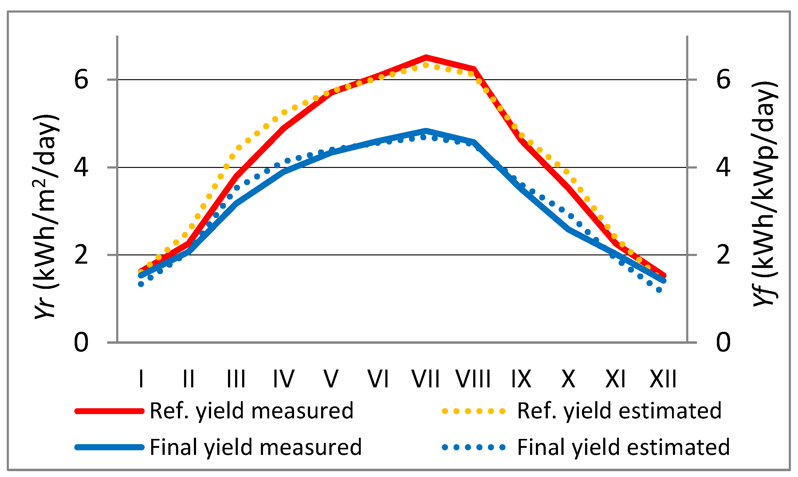
The average value of Y_f in the respective period was 1174.4 kWh/kWp/year (1183.6 kWh/kWp/year expected according to PVsyst). The maximum value of 1265.3 kWh/kWp/year was reached in the first year of operation, while slightly lower value was achieved in 2017 and 2019. The minimum was reached in the second year and had the value of 1073.4 kWh/kWp/year. According to the daily measurements the average value of the Y_f was 3.21 kWh/kWp/day, while the estimated value was 3.24 kWh/kWp/day. The Figure 4 shows the achieved value of the daily average of the final and reference yield for the 8 years of operation.

In the analyzed period the average value of Y_r was 4.09 kWh/m²/day, while PVsyst estimation was 4.20 kWh/m²/day. The lowest value was in 2013 with 3.90 kWh/m²/day, when the total yearly production was also the lowest. The highest value of the yearly average was reached in 2017 with 4.27 kWh/m²/day, when the total energy production almost reached the maximum value from 2012. During the year, the lowest values are reached in winter months, when most cloudy and foggy days can be expected. The minimum values for the winter period was 1.23 kWh/m²/day. On the contrary, the highest values were registered during summer months. The peak value was achieved in the year 2017 with 7.28 kWh/m²/day.

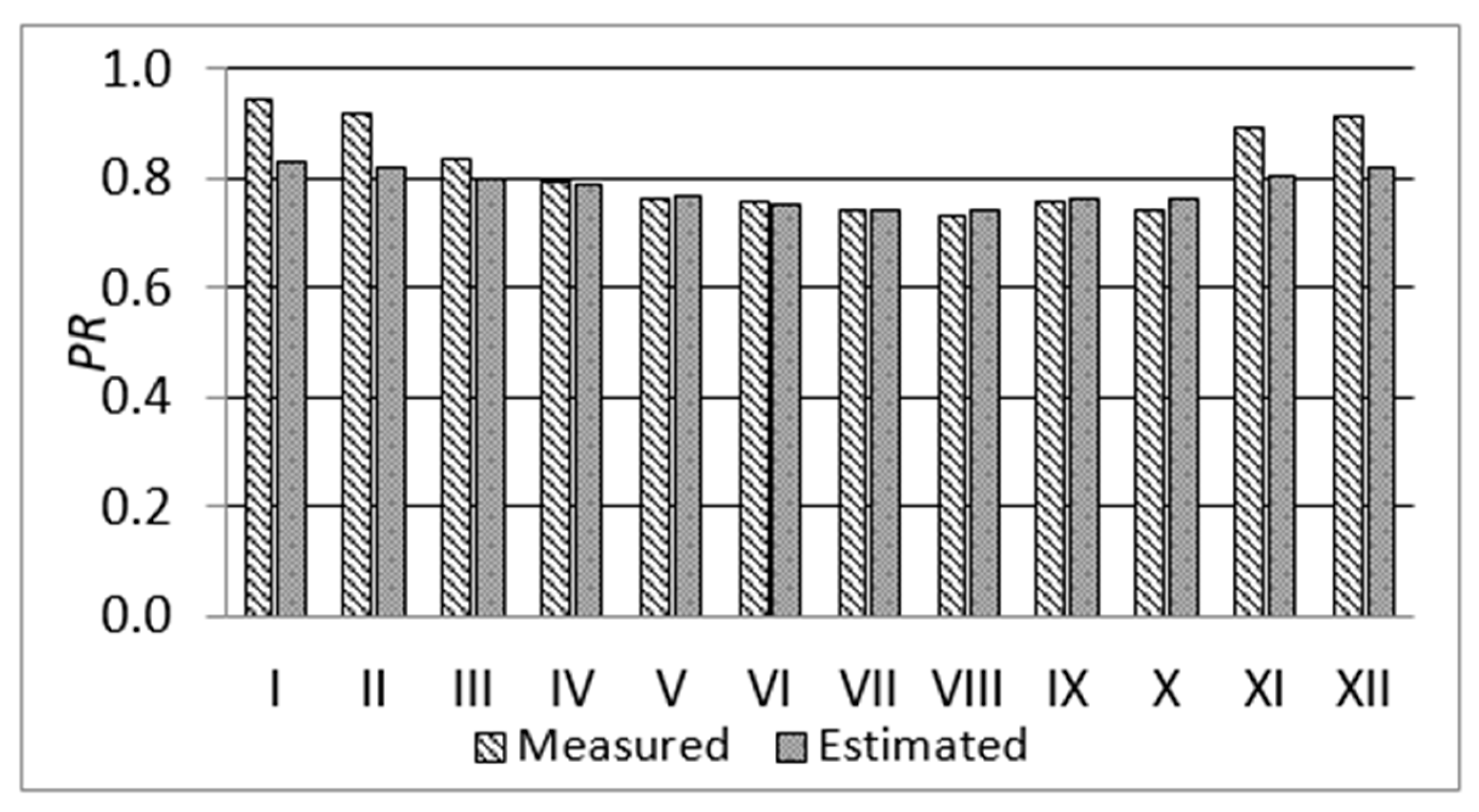
The yearly average value of the PR in the period of analysis was at 0.816, while the PVsyst estimate was 0.782. The maximum yearly value of the PR was achieved in 2106 at 0.844 and the minimum yearly value was 0.769 in 2018. The average monthly values of the PR can be seen in Figure 5, where the calculated values (based on the data from the logger unit) and the estimated values are shown. The values differ significantly in the winter months with approximately 12% difference between the estimated and the calculated value of PR. By the relevant daily measurement data in the PV power plant, when there are no shading of the PV modules and the irradiation level is above 200 W/m² the PR are between 0.83–0.88. During the shading period (before the modules leave the shadow), that can last between 1 h and 2 h depending of the season, there is a significant deviation of this parameters. The higher differences between measured and estimated values in winter months, and lower values of PR during shading conditions are the consequence of specific behavior of the shaded PV module, but also the position of the irradiation sensor. Influence of the irradiation sensor position is especially high in the winter when shading conditions last longer and the days are shorter.

In the

Table 2. The FTS PV power plant capacity factor.

Years	2012	2013	2014	2015	2016	2017	2018	2019
CFYEAR	0.1440	0.1225	0.1290	0.1367	0.1346	0.1425	0.1284	0.1315

the values of CF_YEAR are presented for every year in the respective time interval. The average value of CF_YEAR is 0.1337.

6. Experiments at the PV Power Plant

In the PV power plant, during 8 years of operation, several experiments were conducted where the daily change in inverter performance was monitored, inverter saturation operation was analyzed, the influence of the PV module soiling, ageing and soil ration (SR) were determined. The measurements were performed using a device for measuring PV array characteristics, the SOLAR IV (HT Italia Srl, Faenza, Italy) and remote unit SOLAR-02 (HT Italia Srl, Faenza, Italy). In addition, using MPP300 (HT Italia Srl, Faenza, Italy) with the previous devices the complete yield test of the three-phase inverter can be performed.

6.1. Daily Inverter Operation Analysis

In this section, the daily measurements that were conducted on 7th of July 2015 are presented. The power plant started generating electrical energy at 5:20 and continued the operation until 20:10, having operated for 14.16 h in total that day. Due to logger memory, limitation the sampling period could be no lower than 2 min. The following values have been logged: minimum, maximum and average values for voltage, current and the power at the DC and AC subsystem, irradiation and the PV module temperature. Using the measurement data, the inverter efficiency, PV array utilization in regard to the STC and inverter PR were calculated and logged.

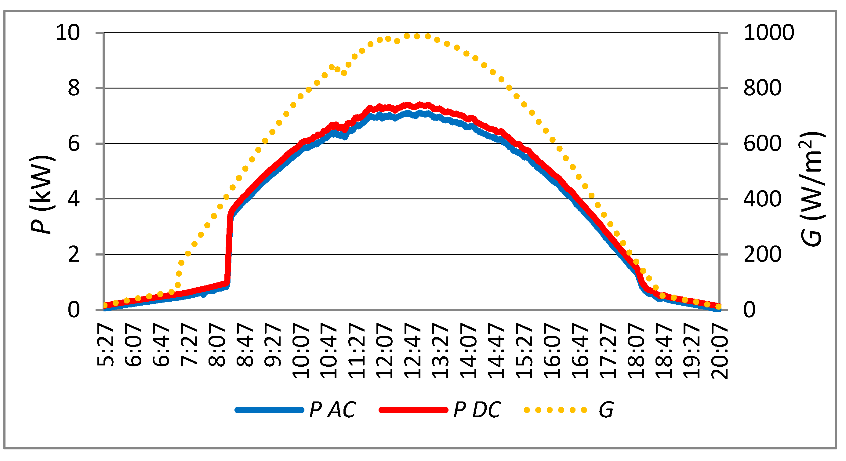
Figure 6 shows the variation of irradiation, inverter input and output power. The spike in inverter power at the beginning of the graph indicates that there is partial shading on the PV array. The irradiation in the shade is increasing linearly, and at the end of the shaded operation period has the value of 69 W/m². At the same time, the temperature of the PV panel is 27.8 °C, output power of the inverter is 437.9 W, while the power of the PV array is 566.4 W. At 7:13 there is an irradiance increase from 69 W/m² to 159 W/m² because the SOLAR-02 irradiation sensor was set up to measure the irradiation of the first module to leave the shade. Due to this and the PV module behavior under partial shading conditions the increase of the PV inverter power occurs much later and not at the same instance as irradiance increase. In the interval from 8:21 to 8:25 the last PV module leaves the shadows and both PV arrays are fully irradiated. Then the PV array power increases rapidly from 960 W to 3379 W. The last measurement for the Sensorbox, the PV power plant irradiation sensor, before leaving the shade was at 97 W/m², while the irradiation was 377 W/m² when the last PV module exists the shadow.

The difference between input and output power of the inverter is clear, especially during the highest irradiation periods (G > 500 W/m²). The PV module temperature in that varied from 46.1 °C (air temperature 30.6 °C) up to maximum of 70.7 °C (air temperature 40.6 °C) in 13:37. For the same irradiation levels the temperature of the PV modules are higher in the afternoon hours.

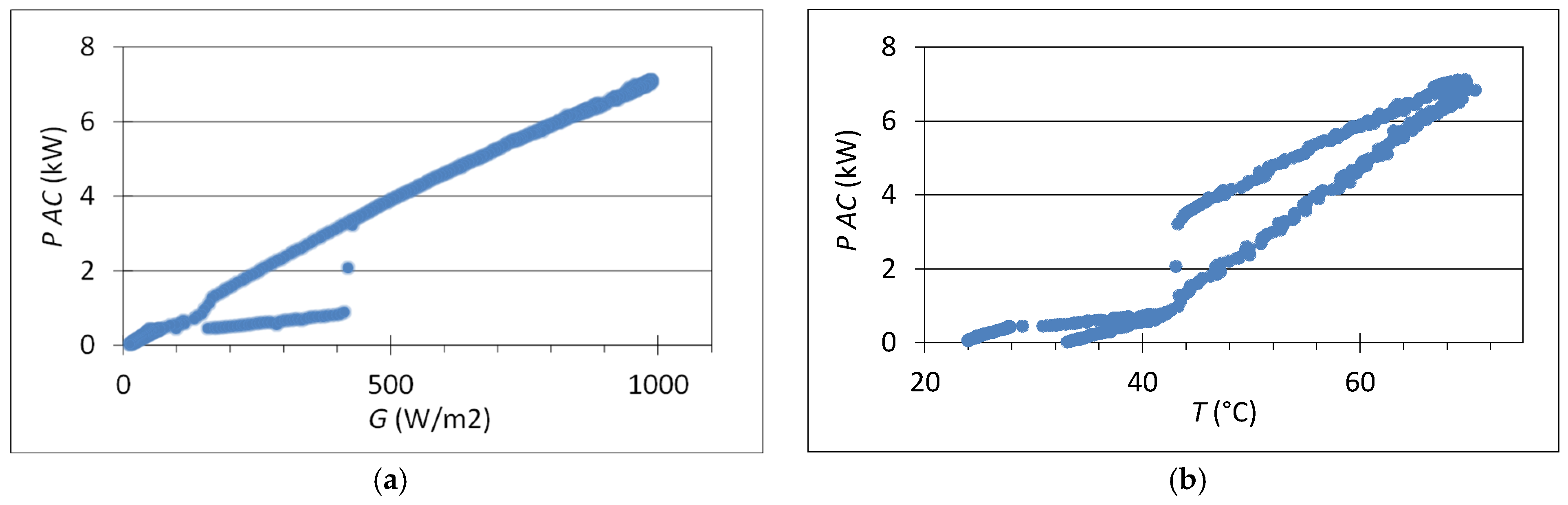
Figure 7 shows the variation of inverter output power in regard to ambient conditions. In Figure 7a the dependency on irradiation is presented, while Figure 7b shows the output power dependent on the temperature. The characteristic in Figure 7a has a very distinct outlook (with dual values for certain irradiation levels). This occurs due to shading of the PV modules, when PV arrays for the same irradiation have lower power output (lower dual values). The linear characteristic is acquired when no shading occurs at the PV modules. In Figure 7b, four distinct parts can be noted (linear parts with different slopes). Two lines with the smallest slope represent the variation of the inverter power (less than 1 kW) for the morning and evening period when the temperatures are also low (less than 40 °C). The other two lines differ in power due to temperature difference in the different parts of the day. For the same irradiation and different temperatures (pre-non and afternoon) we can have different inverter output power.

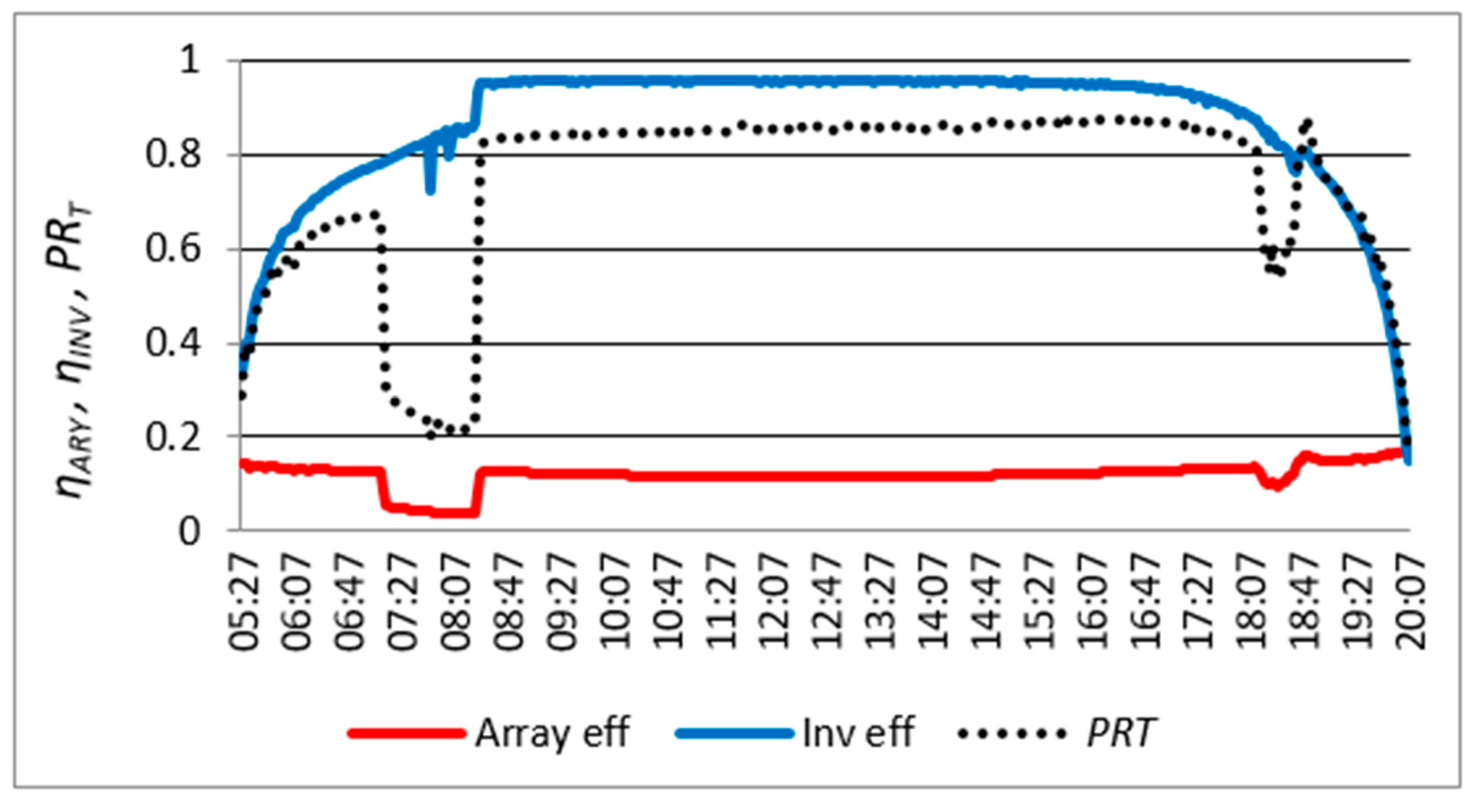
Daily inverter efficiency variation, PV array efficiency variation and PR are presented in Figure 8. Inverter efficiency has an increasing tendency until both PV arrays leave the shade. After this spike in the efficiency it remains constant until a decrease in efficiency occurs late in the afternoon. Maximum inverter efficiency was 96%. Average efficiency was 86% in before noon and 94% in the afternoon, with the daily average of 90%. PV array efficiency in the early morning hours is increasing, however at 7:13 there is a quick decrease followed by a continuous slight decrease. This can easily be explained by the fact the irradiation sensor of the Solar-02 has left the shade and the irradiation is continuously increasing. Sharp increase in efficiency occurs when both PV arrays have left the shadow. Consequently, when the PV array efficiency is lower, the PR value also decreases as evident from Figure 8. The average values of PR before noon, in the afternoon and daily are respectively 0.77, 0.85 and 0.81.

The measurement results from the PV power plant data loggers do not show the sharp decrease in PV array efficiency and PR due to the position of the irradiation sensor of the acquisition system. This irradiation sensor leaves the shade almost at the same time as both PV arrays, and therefore the increase of the PV array power due to shading and the irradiation increase simultaneously and proportionally.

Late in the afternoon, there is one more PV array efficiency and PR drop lasting for 35 min. This is also due to the partial shading of the PV arrays and the characteristics return to expected path after all the PV modules are shaded again. In this case the decrease is not due to the position of the sensor but rather to the inverter operation and maximum power point tracking. When the shading occurs, there is a slight change in the PV array current and a higher voltage variation. The current is decreased by 13% for a short time (lasts about 6 min), while the PV array voltage drop for 100 V and 218 V, i.e., 20% and 42% respectively. When the partial shading conditions pass (i.e., when all PV modules are in the shade) the voltage variation returns to normal, voltage start decreasing and when it reaches the minimum operational voltage the inverter shuts down.

6.2. Saturation

Due to high inverter power sizing factor when there are high irradiation conditions, especially when there are lower ambient temperatures the inverter operates in saturated conditions. Considering the climate in Republic of Serbia, the inverter saturation can occur in March, April and September. During the eight-year period, the ambient conditions for saturation occurred during 14 days, which makes 0.55% of the operating days. In the spring of 2013, the inverter was in saturation the most times, with five occurrences whereby the inverter output power reached 8 kW. The saturation is reached at noon when the irradiation is between 1000–1050 W/m². The PV module temperature was in range from 35 °C to 40 °C.

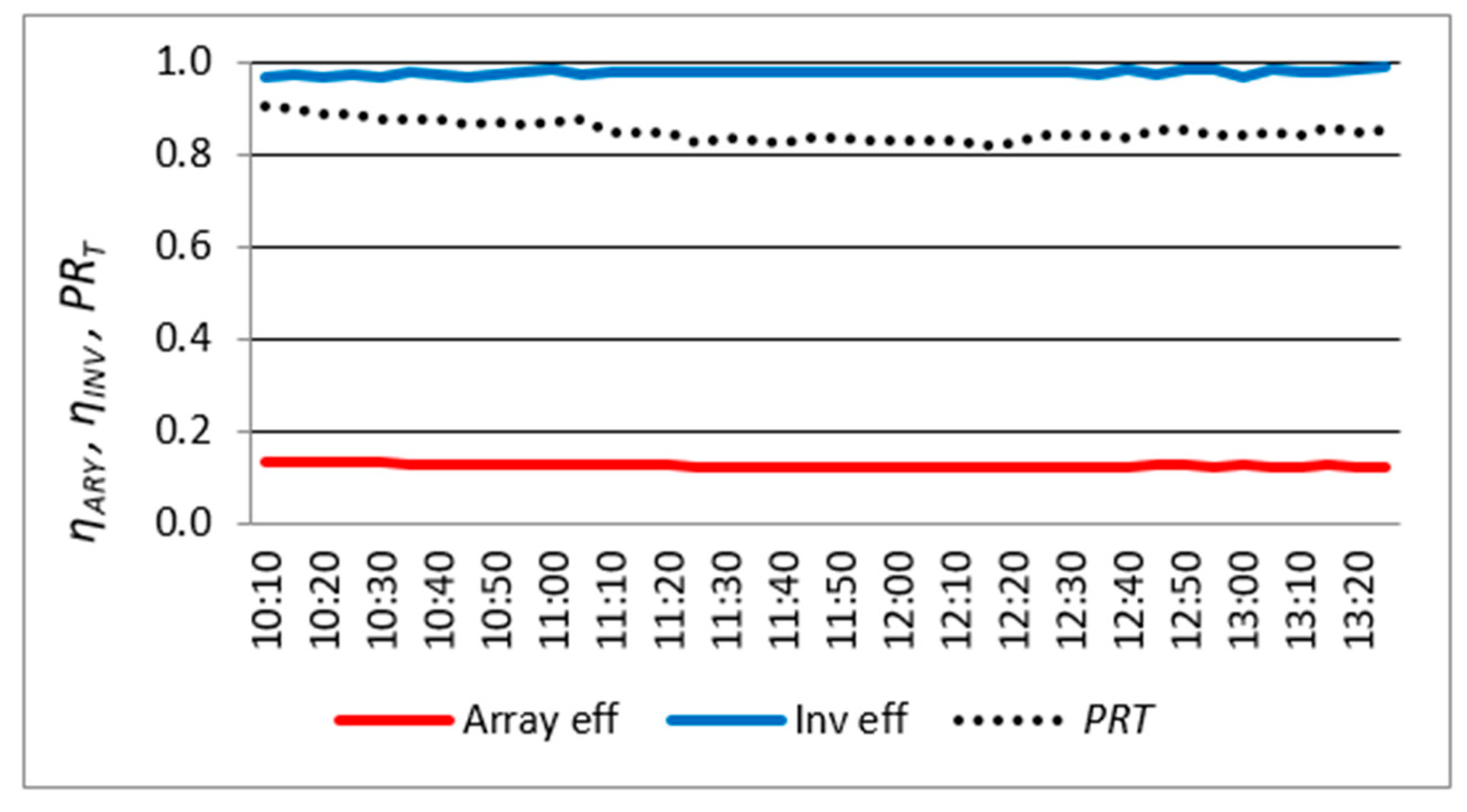
The analysis of the inverter saturation influence on the power plant performance was done for the 25th of March 2016. For this particular date, the inverter was saturated from 11:10 to 12:25. During the inverter saturation, the PV module temperature was between 36.9 °C and 37.3 °C. According to ambient conditions, PV module temperature coefficient (−0.45 %/°C) and an average PR_T the PV array module can be estimated at 8630 W. The inverter output power during saturation was 8008 W. The variation of the inverter efficiency, PV array efficiency and the PR_T are presented in the Figure 9. The efficiency of the PV array, in comparison to STC, slightly decreases before the saturation. During and after saturation it ranges between 12.1% and 12.6%. The average value of PR_T during saturation is 0.834. According to the analyzed data it is easy to conclude that there is no deterioration of the power plant parameters during saturation. In a rare occasion when the inverter is saturated there are no visible change in power plant performance.

6.3. Soiling and Power Decrease of PV Modules

After four years of PV plant operation a random four PV modules were selected PVP1, PVP2, PVP3 and PVP4 (two in each array) in order to determine the influence of soiling on the power decrease. The measurement device logs instantaneous power and the power normalized to the STC.

Table 3. The influence of soiling on the PV modules power.

PV Module	State	P (W)	ΔP (%)	SR
PVP1	Soil STC	219.07	4.5	0.955
	Clean STC	229.35
PVP2	Soil STC	215.29	5.7	0.943
	Clean STC	228.31
PVP3	Soil STC	217.26	5.3	0.947
	Clean STC	229.32
PVP4	Soil STC	218.74	4.4	0.956
	Clean STC	228.77
		Average:	5.0	0.950

presents the power normalized to the STC for soiled and clean PV modules and soiling levels according the Equation (15). The average soiling levels of the PV modules is determined at 5%, which is higher than a standard default value of 3% used by the PV software to determine the estimated PV power plant production. It is important to note that the PV modules were first cleaned (considering the beginning of operation time) when the experiments to determine the SR were carried out.

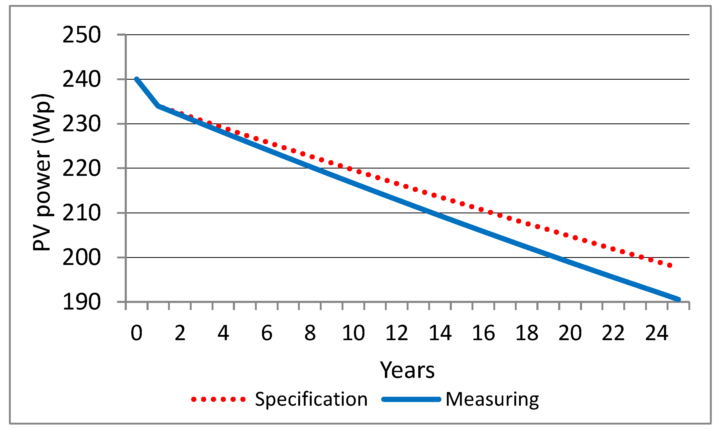
After seven years and five months of the power plant operation PV module power was measured in order to determine the aging effect. The DR parameter was calculated in regard to the rated PV module power and blitz test power. According to the specification the rated PV module power is in the range of ±3 %Pn. PV module power according to blitz test are in range of ±1.5 %Pn.

Table 4. PV module blitz test and measurement power and degradation rate level.

PV Module	Blitz Test P (W)	Measurement P (W)	DR Blitz Test (%)	DR Rated (%)
PV1	239.73	221.96	7.41	7.52
PV2	238.77	219.74	7.97	8.44
PV3	238.49	220.67	7.47	8.05
PV4	240.99	221.85	7.94	7.56
PV5	239.47	220.54	7.90	8.11
PV6	239.,2	221.38	7.45	7.76
PV7	239.62	220.22	8.10	8.24
average:	239.47	220.91	7.75	7.95

shows the blitz test PV module power, PV module power measurement results and DR value for seven tested PV modules (PV1 to PV7). Average value of DR in regard to the rated power was 7.95%, while in regard to the blitz test it was 7.75%. The manufacture states limited power warranty for the rated power. According to this parameter in the first year the maximum allowed power decrease is 2.5% and 0.7% for every consequent year until 25th year. When calculated at the moment of testing the DR should be at 6.98%.

Power decrease estimation in the expected life span of the power plant (25 years), according to the specifications and the measurements can be observed in Figure 10. After 25 years the PV module power will be 197.7 Wp according to the specifications and 190.6 Wp according to the measured DR.

Inverter coefficient, at the power plant design stage, is defined according to the PV module rated value. However, since there is a decrease in the PV module power during exploitation, value of the K_inv also decreases. According to the measurements of current values for the inverter coefficient is estimated at 1.11. If the PV modules are not replaced in the 25-year life span, the expected value of the K_inv will be 0.95.

7. Discussion

This paper analyses the operational parameters of a PV power plant over an 8-year period of operation, which allows for a unique perspective of PV system operation to be considered related to the existing literature where mostly one-year operation is considered. The one-year period, while being most common, may lead to some inaccurate assessment of the most important operational parameters. There is only a handful of papers that analyze longer period of PV plant operation, such as [36]. From the perspective of the power plant analyzed in this paper, for example, if the year 2011 was selected the highest value of Y_f is 1265.3 kWh/kWp/year, while for the year 2012 the parameter Y_f would be 1073.4 kWh/kWp/year. This makes the difference of 15.2% and the average value for the analyzed period was 1174.4 kWh/kWp/year. Other parameters behave very similarly, hence the importance of the longer analysis period offered by this paper.

Reference [18] also analyzes the operation of a PV power plant in Serbia, but the analyzed period is one year and the location of the power plant is in Nis, the city 300 km to the south of Novi Sad and the respective PV plant analyzed in this paper. Both power plants have a similar design, with south orientation and almost the same elevation angle (Novi Sad 30°, Nis 32°). The analyzed FTS PV power plant in Novi Sad has K_inv = 1.2 and operates under partial shading conditions in the morning hours, while in the PV power plant analyzed in [18] there is no shading conditions and the corresponding K_inv = 1.0. The eight-year average value of Y_f for the respective location is 3.21 kWh/kWp/day, while the estimated value was only 0.93% higher. Measured and estimated value of Y_r, are 4.09 kWh/m²/day and 4.20 kWh/m²/day respectively, which makes a difference of 2.69%. The level of correlation between the estimated and the measured value with the certainty interval of 95% for Y_f and Y_r can be concluded to be very high with the values of 0.988 and 0.994 respectively. This is significantly higher than the 0.576, which is a limit value for the certainty limit for 12 samples (12 months). The accurate correlation between estimated and achieved values of PV power plant parameters can be achieved only after longer period of analysis (5–6 years). For the analyzed year (2013), PV power plant from Ref. [18] has Y_f = 3.18 kWh/kWp/day and Y_r = 3.81 kWh/m²/day, while for the same year PV power plant in Novi Sad achieves the values of Y_f = 2.93 kWh/kWp/day and Y_r = 3.90 kWh/m²/day.

When the value of the PR is considered for the good performance PV power plant, they should usually range between 0.75 and 0.85. Below these value performances are considered as poor, while over the 0.85 the performance can be considered excellent. According to the measurements the calculated value of the average yearly PR is 0.818, which is 4.6% higher than the PVsyst estimated value.

The PV power plant in Nis achieved the value of PR at 0.936 for the year 2013, while in Novi Sad it was at 0.793 for the same year. The value of Y_f is higher and the value of Y_r is lower for the PV power plant in Nis, which leads to the higher PR value. However, the higher value of K_inv means higher energy generation per kW of installed inverter power, which leads to the increase in energy generated by the PV power plant. This can easily be explained by the longer inverter operation period (earlier turn on and later turn off times), higher power during the operation and partial compensation of shading losses. In that regard, the average energy generation per kW of inverter installed power for the FTS power plant in the analyzed period was 1409.3 kWh/kW, while for the K_inv = 1 it would have been at 1174.4 kWh/kW. Therefore, the increase of 20% in inverter power sizing factor leads to the increase of 16.7% in the generated energy.

As an added benefit, every increase in energy generated from renewable energy sources leads to the reduction of fossil fuel emission. By the relevant daily measurement data in the PV power plant, when there are no shading of the PV modules and the irradiation level is above 200 W/m² inverter efficiency and PR are between 90.4–96.0% and 0.83–0.88, respectively. During the shading period (before the PV modules exit the shadow), that can last between 1 h and 2 h, depending of the season, there is a significant deviation of these parameters. This is mostly due to specific behavior of the shaded PV panel, but also due to the position of the irradiation sensor that significantly influences the PR. Influence of the irradiation sensor position is especially high in the winter when shading conditions last longer and the days are shorter.

In a rare occasion when the inverter is saturated there are no visible change in power plant performance, (which is significant considering high K_inv). According to the PV module power at the STC, the saturation of the inverter can be expected when the irradiation is around 1000 W/m² and the temperature of the PV modules is lower than 45 °C, i.e., air temperature is lower than 20 °C.

The soiling levels of the PV modules is determined at 5%, which is higher than a standard default value of 3% used by the PV software’s to determine the estimated PV power plant production. It is important to note that the PV modules were first cleaned (considering the beginning of operation time) when the experiments to determine the SR were carried out. The parameter K_inv can also compensate for the losses attributed to the soiling of PV modules, same as in case of electrical and non-electrical losses.

When the measurements results are considered, the power deterioration (regarding the panel aging) is slightly higher than the manufacturer data states. The estimated PV panel power in the 25th year of operation will be about 3.6% than the manufacturers guarantee. The PV panel power decrease in 25 year will result in inverter power sizing factor dropping from 1.2 to 0.95 for the respective PV power plant, if the inverter or the PV modules are not replaced. In that regard, the selection of high value of inverter power sizing factor at the beginning can be fully justified, since towards the end-of-life expectation influenced by PV module aging this value will drop close to 1, still having significant influence on the increase in production and the reduction of the harmful gases emission.

8. Conclusions

The measurements results and the performance analysis of the FTS power plant in Novi Sad showed its good performance, despite the high losses due to operation under partially shading conditions and high inverter power sizing factor. By comparing the values of Y_r from this paper to the different papers with locations worldwide, a conclusion can be made that Republic of Serbia has very significant solar energy potential. The values of Y_f and PR for the respective PV power plant are higher than for other power plants with similar potential. The estimated values of Y_r and Y_f, using PVsyst software, can be considered accurate to the actual average values with high level of certainty.

The main conclusions of the paper are:

• In order to have the best representative results for analysis a long-term (multi-year) parameter measurement is necessary.
• Some parameters, such as Y_f and SP, are not influenced by the inverter power sizing factor irrelevant to the system environment.
• The most important parameter (energy generation) is highly influenced by the inverter power sizing factor value.
• The saturation effect due to high value of inverter power sizing factor does not influence the inverter efficiency negatively.
• Due to PV module aging, higher value of inverter power sizing factor allows higher total PV module power at the end of life point of PV system.
• The saturation effect is more pronounced at the beginning of operation, while with PV module aging this situation occurs less often.
• PV module soiling reduces the energy output by 5% if the PV module are only treated by natural rainfall.
• Considering the relative immaturity of the technology (rapid development only in the last decade), the concluded experiments give significant contribution to the knowledge accumulation in the topic of inverter operation under partial shading conditions and inverter saturation, PV module power degradation due to aging and soiling in the urban installations.

To summarize, the paper shows that the high inverter power sizing factor of a PV power plant that operates in severe partial shading conditions can achieve the expected energy yield, high performance and can operate without technical difficulties.

Building on the presented results, future research will include further investigation of the soiling influence on the PV array power with special reference to mitigation possibilities. Additionally, PV module aging was just briefly touched on by this paper, while future research will include extensive testing of different parameters that can influence module aging using advanced software solutions such as ComSol to verify the experimental (field) results. Most importantly, since the PV power plant operates under partial shading conditions, the model for the PV array reconfiguration in order to mitigate the shading effect has already been developed [27]. Future research will assume the experimental verification of the proposed reconfiguration using automatic reconfiguration matrix, but it will also propose a reconfiguration matrix in order to vary the value of the K_inv during the PV power plant operation in order to maximize the inverter output power throughout the day.