Benefit Evaluation of PV Orientation for Individual Residential Consumers


1
EELab/Lemcko, Department of Electromechanical, Systems and Metal Engineering, Ghent University, 8500 Kortrijk, Belgium
2
EELab, Department of Electromechanical, Systems and Metal Engineering, Ghent University, 9052 Ghent, Belgium
*
Author to whom correspondence should be addressed.
Energies 2020, 13(19), 5122; https://0-doi-org.brum.beds.ac.uk/10.3390/en13195122
Submission received: 30 August 2020
/
Revised: 21 September 2020
/
Accepted: 28 September 2020
/
Published: 1 October 2020
(This article belongs to the Special Issue Photovoltaic Systems: Modelling, Control, Design and Applications)
Abstract
:Photovoltaic (PV) installations located in the northern hemisphere must be oriented to the south in order to obtain maximal annual yield. This is mainly driven by the remuneration mechanisms which incentivize maximal energy production to a certain extent. Nowadays, such support mechanisms are declining or even phased out in many countries. Hence, self-consuming the produced energy is getting more viable. In order to match better the load demand pattern, the azimuth angle of a PV installation could be changed or oriented towards multiple directions. This article investigates the benefits of PV installations facing other directions than the south. Therefore, the Hay & Davies transposition model has been used to calculate the in-plane irradiance, as it is found in the literature to be the most accurate for non-south faced PV installations. In order to determine the benefit, a large dataset of real measured consumption profiles has been used and then divided according to their annual consumption. Large consumers with an oversized east/west-oriented PV installation especially take advantage. The self-sufficiency index (SSI) is found to increase with almost 0.94 percent points, while the self-consumption index (SCI) increases with 6.46 percent points. The peak reduction is assessed by calculating the annual moving average of the month peaks. It is found that this moving average month peak reduction is marginal. Lastly, the reduction in storage capacity is found to be not that significant, although in terms of battery utilization it is found that the number of discharge cycles is reduced with 6%.
1. Introduction
The global warming is stimulating countries to take actions to reduce their CO2 emissions. Many countries are taking measures to this end and have introduced national energy and climate plans [1]. Electricity generation that causes an important part of the CO2 emissions should shift from fossils to renewable energy [2]. Today, solar energy is one of the fastest growing renewable energy technologies and is today already one of the cheapest energy forms [3]. Moreover, research in new and more efficient technologies and materials is nowadays still ongoing [4,5]. Worldwide, almost 75 GWp of utility-scale photovoltaic (PV) installations has been built in 2019 and 40 GWp of distributed PV [6]. Distributed PV is mostly mounted on the roof of a residential or industrial building with fixed-tilt panels. Tracking systems are typically not used in residential applications in west and north Europe, mainly because it is not cost-efficient [7].
The Air Mass (AM) of the sun rays is minimal during the noon and amounts 1, which means that the path length the light takes through the atmosphere is then minimal. The longer the path length, the higher the light absorption of the atmosphere and thus the lower the solar energy reaching the earth. The AM increases as the sun angle is approaching the horizon. This explains why south faced solar panels achieve the highest yield on year basis for countries situated in the northern hemisphere [8]. Another critical parameter when installing fixed-tilt panels is the tilt angle. Jacobsen et al. showed that there is a linear relationship between the geographical latitude and the optimal tilt angle for low latitudes in the northern hemisphere. However, for high latitudes, air pollution, cloud cover, and haze affect and decrease the optimal tilt angle with 10° to 20° compared to the latitude. The lower the tilt angle, the more diffuse irradiation it will receive [9,10].
The benefit of striving to maximal yield is mainly driven by the remuneration mechanisms. In many countries, PV installations can sell their not consumed energy back to the local grid according to the contracted feed-in tariff (FIT). For instance, in Germany and France, the FIT is guaranteed for 20 years, but the tariff is decreasing every year [11,12]. In the United Kingdom, FIT has been closed from 1 April 2019 on. The support scheme has been replaced by the Smart Expo Guarantee (SEG). This incentive legally obliges energy suppliers to pay their consumers for each unit of generated electricity [13,14]. The tariff rate can be freely chosen by the supplier and could be time dependent in the future. In Flanders (Belgium), PV installations built before the end of 2020 will probably benefit from net metering scheme support from the last 15 years. This decision must still be confirmed by the Constitutional Court. The support consists of a system in which the injected energy into the grid is deducted from the electricity consumed [15]. As of 1 January 2021, this support will be replaced by a one-off investment grant. Similar phasing out trends of FIT and net metering schemes are noticeable in many other countries [16]. The support schemes are evolving in a way that self-consuming the produced energy is getting more viable.
The self-consumption index (SCI), i.e., the ratio between the direct consumed PV energy and the overall produced PV energy, amounts for a residential PV system of 1 kWp per MWh consumption typically 30%. The self-sufficiency index (SSI), i.e., the part of the consumption that is supplied by the PV installation, amounts for the same system also typically 30% [17]. Higher SCI and SSI could be achieved by foreseeing a storage unit, by shifting the consumption in time, by spreading out, or shifting the PV energy in time. The latter can be reached by changing the azimuth angle or face the PV panels to multiple orientations. Only a few papers have been examining the impact of PV orientation on SSI and SCI. Weniger et al. [18] investigated the SSI of a residential grid user with a single-oriented PV in function of the azimuth angle, and determined that the highest SSI could be reached for south-oriented PV. In [19], both indexes, SCI and SSI, have been investigated for PV oriented to south, east, west, and east/west. The SCI increased with 6 percent points (absolute percentage difference) for east/west-oriented PV compared to south-oriented PV. However, the SSI decreased with almost 1.5 percent points. Both authors simulated the in-plane irradiation using meteorological data and the Klucher model for transposition of the diffuse irradiation. The consumption profiles are either based on reference load profiles or are obtained by measurement of a private household. Lastly, the study [20] used measured irradiation data of different azimuth angles and a set of 74 load profiles to determine SCI and SSI. An increase of the SCI of almost 14 percent points is reached for E/W-oriented PV compared to south-oriented PV. The SSI increased with 1.1 percent point. The authors concluded that east/west- and southeast/southwest-oriented PV is economically slightly more beneficial when considering a declined FIT. Furthermore, the authors suggested that east/west orientations would also reduce the cost for storing the PV energy. The authors in [21] investigated the impact of PV orientation on the low voltage distribution grid. They found that deviating the azimuth angle slightly from the south reduces the grid losses and the curtailment losses due to overvoltage. However, the produced energy reduces to a larger extent which makes this not favorable. On the other hand, it was found that changing the tilt angle is more effective as it leads to lower grid losses for a small decrease in energy production.
The calculation of the in-plane irradiance is mostly performed by using measured irradiance components with diffuse horizontal irradiance and direct normal irradiance. Subsequently, transposition models are used in order to estimate the in-plane irradiance to any desired tilt and azimuth angle. Simple models, using straightforward geometrical formulations, could be used with the assumption that the diffuse component has an isotropic distribution over the hemispherical sky. However, this could introduce significant errors as the sky light is anisotropic at many instances. Several transposition models have been proposed in the literature: Perez [22], Klucher [23], Reindl [24], and Haydavies [25]. The study [20] investigated the sensitivity of different models with respect to the tilt and azimuth angles. Depending on the climate, the reflection, the tilt, and azimuth angle certain models perform better than others.
In this study, a benefit evaluation of PV orientation will be performed for individual residential consumers. The PV production will be calculated using the most appropriate transposition model based on measured climate data on a site in Flanders. By using these profiles, SCI and SSI will be calculated and compared to the SCI and SSI obtained by using measured PV production profiles. The study will be based on a large dataset of residential consumption profiles originating from two towns in Flanders which will be divided into three consumption classes as defined by Eurostat [26]: small, medium, and large consumers. The possible benefits of oriented PV for residential consumers could be mainly divided into following three aspects:
- SCI and SSI: As discussed before, due to evolution of the remuneration mechanisms, SCI is getting more important than the produced PV energy. Furthermore, the higher the SCI, the lower the amount of injected energy to the local grid. In Flanders, injection charges pro rata the injected energy will be applied for residential grid users. With respect to the SSI, it is obvious that end users want to minimize the purchased energy from the grid and thus maximize this value. Both indexes strongly depend on the household’s electricity consumption behaviour. This emphasizes the importance of using real measured load profiles. This analysis will be performed separately for the three different consumption classes in order to detect the particularities for each type of consumer.
- Peak reduction: The distribution grid tariffs in the electricity bill of residential grid users is today mainly based on the amount of energy taken from the grid. However, a tendency to more capacity-based tariffing is noticeable in many European countries. This evolution is mainly driven by the expected increasing penetration of renewable energy in the distribution grid and the electrification of mobility and heating [27,28]. By introducing capacity-based tariffs, load shifting and other peak reduction measures could be incentivised. Another more viable solution would be to optimize the orientation of the PV panels in order to reduce the morning and/or evening consumption peaks extracted from the grid. An analysis will be performed to quantify the peak reduction for different type of consumers.
- Save in storage capacity: The general aim of integrating storage facilities is to increase SCI and SSI. By orienting the PV panels in an appropriate way, the SCI and the SSI could already be increased without foreseeing any storage facility. This means that, for a certain desired SSI, a smaller storage capacity could be sized when the PV panels are oriented for instance to east/west instead of to the south.
The first two aspects have an important impact on the electricity bill while the third aspect will especially affect the investment cost of the storage unit. To the best of the authors’ knowledge, no studies have been published addressing those three aspects, using a validated PV simulation model and a large dataset of consumption profiles. This article should give, based on a thorough analysis, a clear answer to the following question: What are the benefits of orienting PV panels to other directions than the south for individual residential consumers? As the consumption and production data are all originating from specific locations in Flanders, the outcome of this study could strictly only be representative for this region.
In Section 2, the used data and simulation models are presented as well as the followed methodology to obtain the desired results. This includes, inter alia, the modeling of the PV system, the definitions and methods to define SCI, SSI, and consumption peak, and, at last, a few practical aspects. In the third section, the results of the validation are shown as well as the benefits in terms of SSI, SCI, peak reduction, and storage. The section will be ended by a general overview of the possible benefits. The last section consists of a reflection on the investigated aspects and the conclusions of the study.
2. Materials and Methods
2.1. In-Plane Irradiance
The input data for the calculation of the in-plane irradiance consist of two irradiation components. Those components are the diffuse horizontal irradiance and the direct normal irradiance or also named the beam irradiance . These data are provided by the Belgian Royal Meteorological Institute (RMI) together with wind speed measured on 10 m height and the ambient temperature. The data are measured during one complete year and originate from a weather station situated in West Flanders (latitude 50.90° N–3.12° E and 25 m above sea level), which is here considered as the study location. The dataset is based on a 10 min average of the irradiance while the consumption profiles are generally based on averaged 15 min values. In order to compare both on the same time bases, the calculated global in-plane irradiance is resampled to 15 min based averages. The global in-plane irradiance on a tilt angle can be estimated as follows:
where is the tilted direct or beam irradiance, the tilted diffuse irradiance, and the ground-reflected irradiance. Many transposition models have been proposed in the literature to estimate the solar irradiance on a tilted plane using horizontal irradiance components. Only the most commonly used models will be discussed below as they represent the common model types: isotropic, anisotropic with two components, and anisotropic with three components. Furthermore, these models need input data that are normally available at meteorological organizations and so no other measurements are needed.
- -
- Liu & Jordan: This model is the most cited and the simplest isotropic model. This means that it assumes that the diffuse radiation is distributed uniformly over the sky dome. Moreover, it considers the ground reflection to be diffuse [29].
- -
- Klucher: Klucher stated that the isotropic model of Liu & Jordan provides good results for overcast skies but underestimate the radiation for clear and partly overcast skies. To overcome this error, Klucher refined the Temps–Coulson model by taking into account the circumsolar and horizon brightening [23].
- -
- Hay & Davies: The diffuse radiation is here assumed as a combination of an isotropic component and a circumsolar component, without taking into account the horizon brightening. The two compositions of the diffuse radiation are quantified by using an anisotropy index [25].
- -
- Reindl: This model is based on the Hay & Davies model with the addition of diffuse radiation coming from the region near the horizon line. Reindl found that with increasing sky overcast the diffuse radiation increases. Therefore, a modulating factor is included [24].
- -
- Perez: Perez proposed a more detailed analysis of the isotropic diffuse, circumsolar, and horizon brightening radiation. The model takes two sky brightness coefficients into account that are derived empirically [22].
Many studies have been found in the literature evaluating these models [30,31,32]. In the study [33], different transposition models have been investigated for various tilt and azimuth angles for the study location situated in Hannover (Germany). It is found that the deviation of the anisotropic models from the measurements increases with increasing deviation from the south direction. This is explained by the fact that the ratio of direct to diffuse radiation decreases and thus the uncertainty inherent to the transposition model increases. In this study, the Hay & Davies [25] will be further used as it is found to have slightly better results compared to the Reindl model. The mathematical formulation of this model is given below:
In this equation, the three parts, the direct, the diffuse, and the reflected radiation could be clearly perceived. is the ground albedo and is here assumed as a constant value of 0.2 as widely accepted and used in modeling of PV systems. The factor is used to quantify the circumsolar part of the diffuse radiation. represents the extraterrestrial radiation. This is the solar radiation that reaches the outside of earth’s atmosphere (on average 1361 W/m2) and is estimated by following the method of Spencer [34]. is the ratio of tilted and horizontal beam irradiance, or, as it is given here, the ratio between the angle of incidence and the zenith angle of the sun. The angle of incidence will also be used for the calculation of the latest unknown parameter, the tilted or in-plane beam irradiance [35]:
with the zenith angle, the azimuth angle of the sun, and the azimuth angle of the surface. As a convention in this study, the reference of the azimuth angle is defined as the north and is further calculated clockwise. Thus, 0° corresponds to the north, 90° to the east, etc.
2.2. PV System
After having calculated the in-plane irradiance, the AC power output of the system is calculated by using PVLib. PVLib is an open source Python library that contains many models for simulating the performance of PV energy systems [36]. The model describing the electrical performance of individual photovoltaic modules is based on the Sandia Performance Model (SAPM). The model basically reconstructs the IV-curve based on module parameters and the calculated in-plane irradiance, taking into account aspects such as the spectral loss and temperature dependency. The module parameters can be extracted of the module database made available by Sandia containing almost 500 modules of different technologies and power [37]. With regard to the inverter, a model is included in the PVLib library that is based on the model presented by Sandia. It consists of a few basic equations in order to reconstruct the efficiency curve for the appropriated DC voltage [38]. For the simulation, the PV module shown in Table 1 is used.
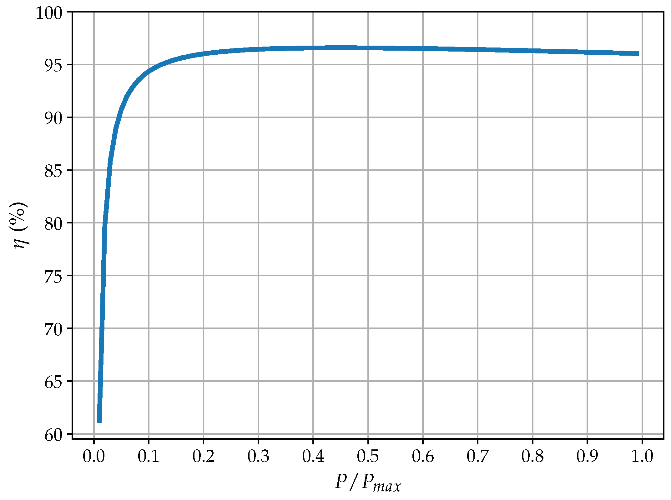
The general efficiency curve of the inverter used for the simulation is shown in Figure 1, with as the produced PV power from DC-side and the nominal inverter AC power. It is worth mentioning that the inverter sizing ratio (i.e., ratio between rated DC-power and the power at AC-side) is assumed to be 1. As high efficiency inverters are considered here, the impact of under- or oversizing the inverter on the annual efficiency is negligible [39,40].
2.3. Consumption Profiles
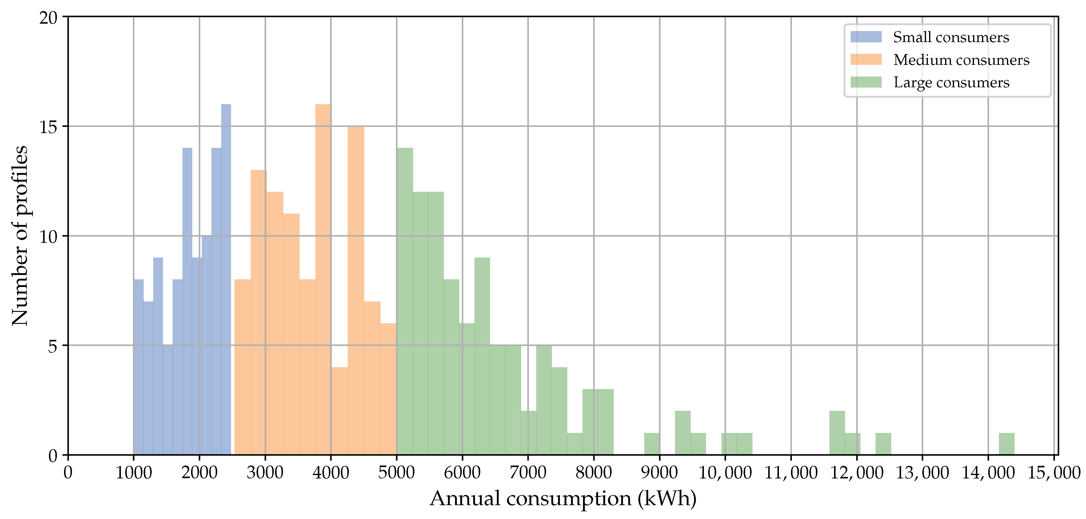
A dataset of almost 1700 load profiles is obtained from the Flemish grid operator Fluvius. The data have a resolution of 15 min and were logged through an automatic measurement reading (AMR) in households situated in two small Flemish towns in a suburban area. After removing the incomplete and inconsistent load profiles, the dataset is divided into three parts corresponding the Eurostat classification [26] and 100 profiles are arbitrarily selected for every consumption class:
- -
- Small consumers: consumption between 1000 and 2500 kWh
- -
- Medium consumers: consumption between 2500 and 5000 kWh
- -
- Large consumers: consumption between 5000 and 15,000 kWh
This subdivision is necessary in order to define the benefit of oriented PV for different types of consumer. The distribution of the annual consumption is presented in Figure 2
2.4. Measurements
Measured PV production profiles are used to validate the in-plane irradiance calculation and the PV system model. These measurements originate from three different residential PV installations collected from pvoutput.org [41], each located in the same area as the weather station. Table 2 contains the technical information of every installation.
2.5. PV Sizing
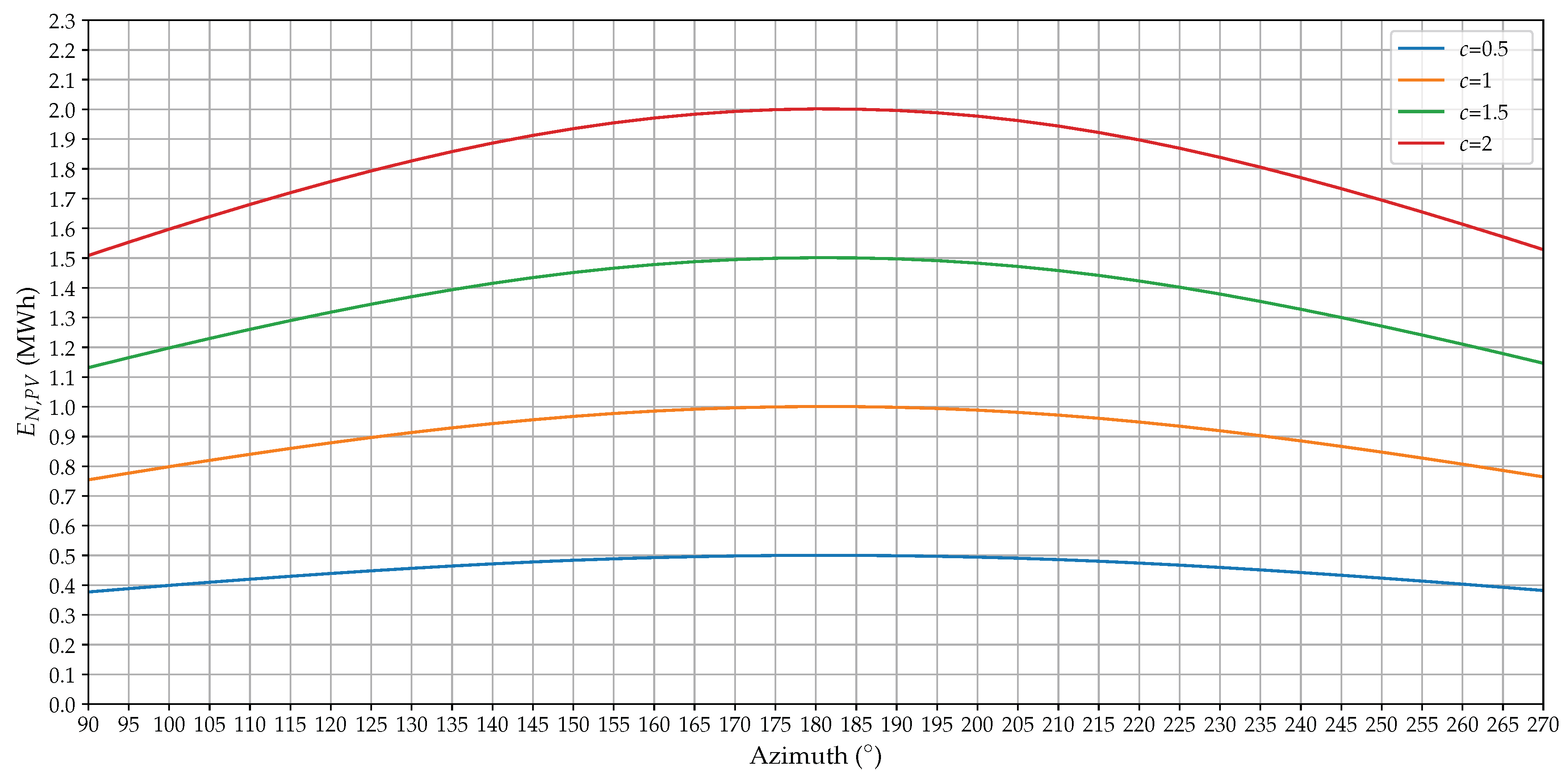
Regarding the sizing of the PV installation, one should pay attention to the fact that using a normalized unit expressed in kWh annual produced energy per kWh annual consumed energy for comparing different PV orientations is misleading. Consider an installation oriented to the east, this will produce approximately 25% less than the same installation facing the south. This would mean that the installation should be sized larger when it is facing other directions than the south in order to produce the same amount of energy. In order to avoid that, the annual production for a certain oriented PV installation x will be normalized to the maximum annual production with the same installation x, thus faced to the south. Furthermore, a sizing factor c is introduced which represents the ratio of the production of a south faced installation to the annual consumption. By doing so, only installations of the same size are compared. The PV output can be calculated as follows:
with as the instantly produced PV power, as the annual production for the most optimal orientation and the annual consumption.
In Figure 3, the variation of the as a function of the azimuth angle and the sizing factor c is shown for 1 MWh. For east and west-oriented PV, the production is approximately 25% less.
2.6. Assessment Criteria
The SCI represents the share of the produced PV energy that is instantly consumed. It is expressed by the ratio of instantly consumed PV energy to the total produced energy. This index will be calculated for each randomly selected load profile from the pool of load profiles in order to represent the SSI in a distribution form. In the first instance, the PV production profile is calculated for the total consumption of residential load i, with . Thereafter, the SCI is calculated for every load and for an azimuth angle . The results of this calculation is a set of values containing the SCI for every residential load i. Lastly, the increase or decrease in SCI compared to a south-oriented PV installation is evaluated by calculating the difference. This difference is expressed in percent points as it represents the arithmetic difference of two percentages. These values will then be presented as a distribution:
The SSI represents the share of the energy consumption that is instantly supplied by the PV installation. It is expressed by the ratio of instantly consumed PV energy to the total demand energy. As for the SCI, this index is calculated for each selected profile in order to represent the SSI in a distribution form:
When considering a PV-storage system, the SSI of the installation could be calculated as follows:
with representing the discharged power of the ESS (energy storage system).
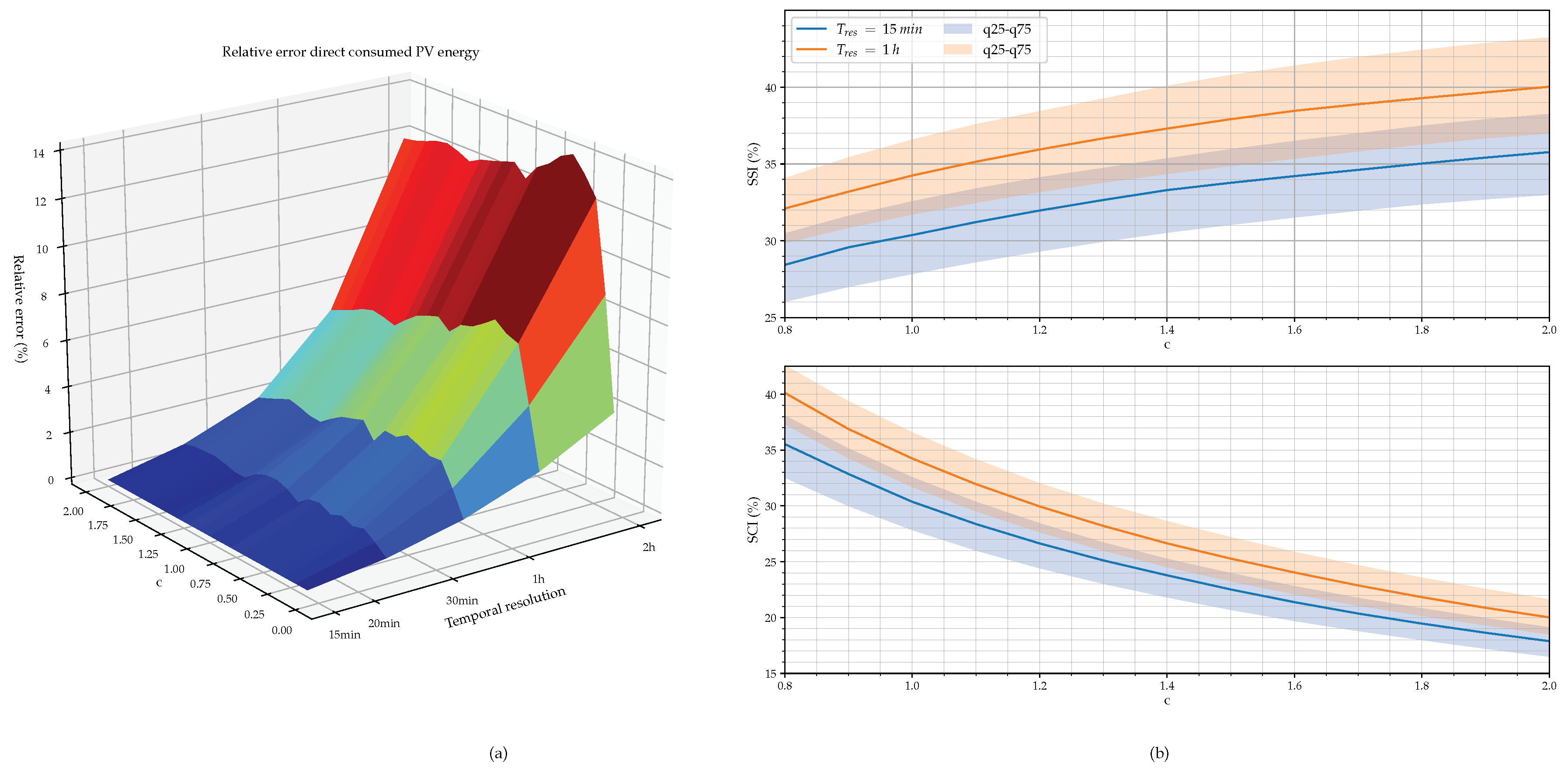
The yield and load profiles used for the calculation of SCI and SSI are measured and then registered at a lower resolution in order to reduce the size of the data. It is obvious that the resolution scale affects the uncertainty of the data as it cannot be known how the profiles behave in real time. Consequently, the presence of errors could not be avoided. Figure 4a shows to what extent the temporal resolution (of load and yield data) could affect the direct consumed PV energy. A south-oriented PV installation and the dataset of large consumers is considered here. The relative error (RE) is calculated by comparing the result to the value obtained with 15 min data. The RE is the largest for small PV installations () and from that point on it decreases slightly with increasing c. For , the RE amounts 6.95% for a resolution of 1 h and 1.12% for a resolution of 20 min.
Figure 4b shows the curve of SCI and SSI and emphasizes the distributional differences related to the temporal resolution. For 15 min-based SSI and , the spread (q25–q75) is 1 percent point larger than for the 2 h-based SSI. For the SCI, this difference amounts to a half percent point.
The authors in [42] investigated this impact for high resolution data of 10 s to 1 h. It was found that for 15 min data the relative errors are usually less than 5% compared to the result obtained by using 10 s data. In [43], the uncertainty of the profitability of PV-battery systems were quantified. By using 15 min data, the battery lifetime is overestimated by 0.7 years.
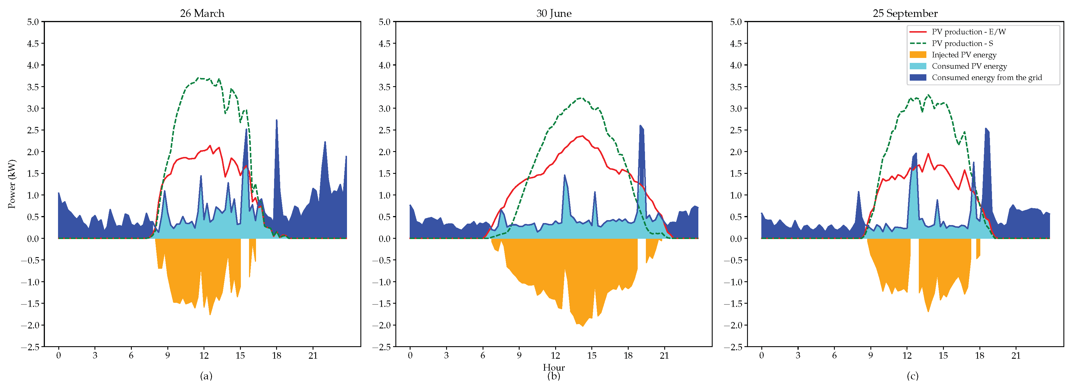
Figure 5 shows the PV production profiles calculated by the model explained above. A profile for a south-oriented PV and for an east/west-oriented PV is shown, each with a tilt angle = 45°. Furthermore, a random selected consumption profile is displayed as well as the instantly consumed PV energy and the injected PV energy. The benefit of oriented PV is clearly visible during the summer day. The production covers a bigger part of the consumption while the lower peak production in months other than the summer season can cause a decrease of the SSI. This will be analyzed further in detail in the next section.
Regarding the peak tariffing for residential grid users, in this study, this will be based on the principle proposed by the Flemish Regulator of the Electricity and Gas Market (VREG) [28]. This tariff component will be for a big part determined by the moving average of the latest twelve month peaks:
with representing the time-of-peak occurrence for each month m.
In this study, the peak reduction will be investigated for a PV installation oriented to the azimuth angle and compared to a south-oriented PV installation. This will again be done for every residential load profile i in order to get the results in a distribution form:
2.7. Practical Aspect
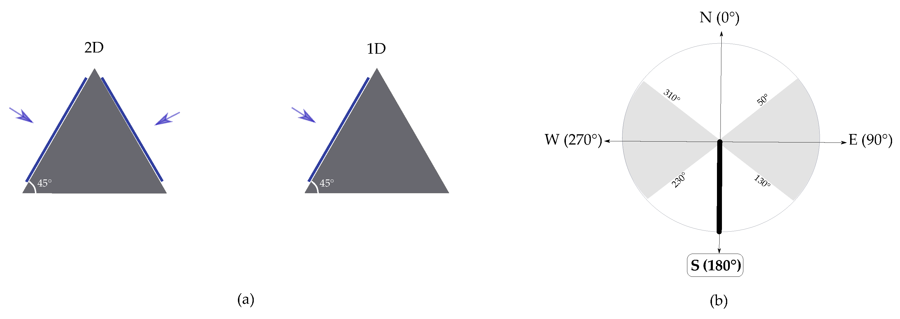
This study will be based on PV installations on pitched roofs faced to one direction (1D) or to two directions (2D) (Figure 6a). The reference base is an installation oriented to the south. For 1D PV installations, azimuth angles () are considered between 90° and 270°, while, for 2D PV installations, the azimuth angles are as described below or displayed in Figure 6b:
Unless otherwise stated, it is considered that, for a 2D PV installation, the roof spacing is equal for both directions, and thus, the same amount of power can be installed ().
Regarding the roof pitch angle, this is set to 45° in order to represent the large number of roof pitches in Western European countries. In [33], it is stated that, in Germany, the houses have a typical roof pitch angle that lies between 40° and 45°. A second reference is a study of the RMI [44] where almost 1450 PV installations spread in Wallonia and Brussels (in Belgium) were monitored. It was found that more than 60% of the monitored installations had a tilt angle of 40°. Notwithstanding this, a sensitivity analysis for different tilt angles will also be performed in order to represent residential consumers with other roof pitches and also to find the most optimal tilt angle. Therefore, the variable should be changed to in Equations (8)–(18) with:
3. Results and Discussion
3.1. SCI and SSI
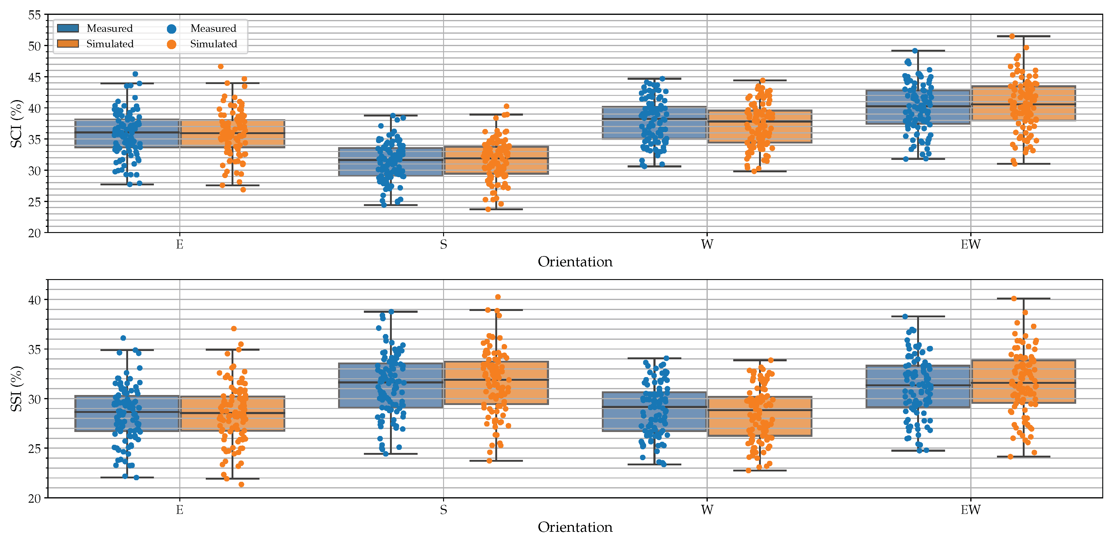
First of all, the SCI and SSI calculated by the measured and calculated production profiles are compared. The calculated production profiles are obtained by using the same technical parameters as described in Table 2. As the installed power is different for the three installations, the production is normalized following the methodology described in Section 2.6, with sizing factor and using the dataset of large consumers. The results are shown in Figure 7 as a boxplot and in Table 3. The colored box is delimited by two horizontal lines with the lower representing the 25th percentile (q25) and the upper representing the 75th percentile (q75). The median (q50) is represented by the middle line and the whiskers are representing the boundaries of the dataset. A scatter of points is overlaid on the boxplot for a better visual representation of the distributional differences.
It is clear that the simulation model is able to accurately estimate the SCI and SSI for east-oriented PV. For the south-, west-, and east/west-oriented PV, very small deviations are noticeable. Furthermore, it can be concluded that the east- and west-oriented PV installation has lower SSI compared to a south-oriented PV installation. In addition, the east/west-oriented PV installation has a slightly lower SSI but a significantly higher SCI. This is the case for both simulation and measurement. More important to notice is the fact that the difference of the median of the simulated and measured SCI and SSI between east/west- and south-oriented PV are quite similar:
- -
- SCI: increase of 8.62 percent points for the measured PV and 8.66 for the simulated PV
- -
- SSI: decrease of 0.19 percent points for the measured PV and 0.31 for the simulated PV
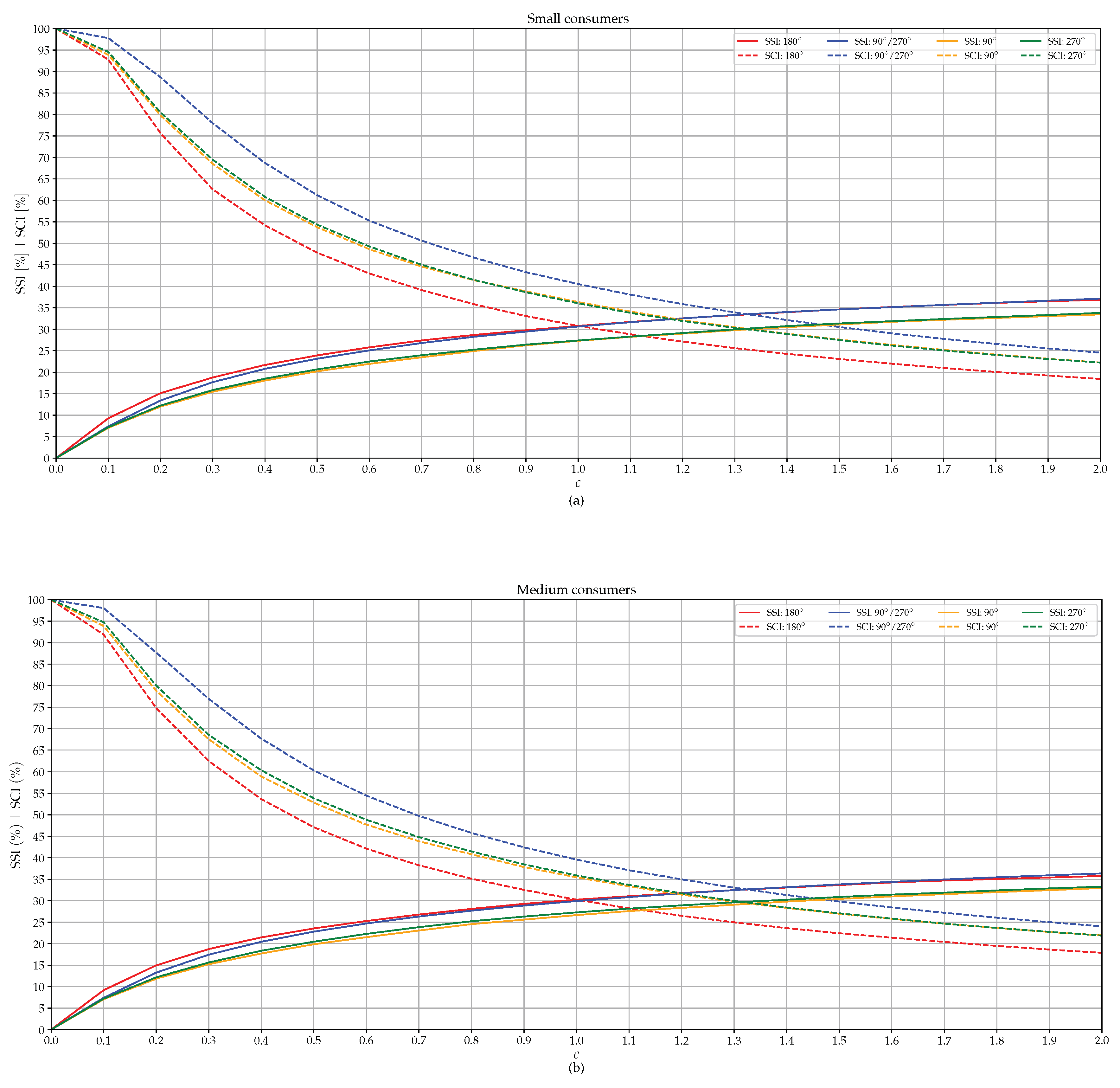
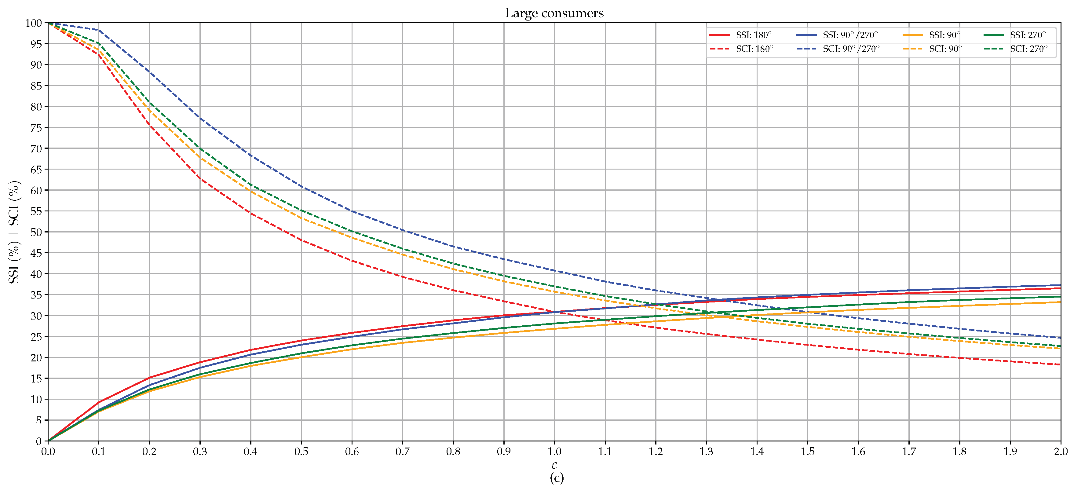
Figure 8 shows the sensitivity analysis of SCI and SSI for different sizing factors c and for different orientations but for the typical roof pitch angle (). This is done for the three types of consumers, small, medium, and large consumers. As the result of this analysis is in fact a distribution, here only the median of this distribution is considered. The larger the PV installation, the lower the SCI and the higher the SSI. However, these curves are not linear but saturate because of the seasonal behavior. For south-oriented PV with , the SCI and SSI amounts to almost 30%. When looking at 1D PV installations, oriented to the east or the west, they both have a higher SCI of almost five percent points compared to a south-oriented PV, irrespective of the type of consumer. Although, regarding the SSI, this is for all cases 3 to 4 percent points lower than a south-oriented PV installation. This is mainly due to the fact that an east- or west-oriented PV installation is only able to cover respectively the morning or evening peak while a south-oriented PV installation reaches higher yields and thus can cover the load on a larger extent.
For that reason, it can be interesting to investigate the benefit of 2D PV installations, east- and west-oriented. It is clear from the graphs that the SCI increases significantly for this configuration. The increase amounts to almost 10 percent points for . This is mainly due to the lower yield rather than a better match between demand and production. For this reason, the SCI could be misleading and is therefore not an ideal parameter to asses the benefit of PV orientation. Nevertheless, the SCI is a good metric to evaluate the amount of the injected energy to the grid. Regarding the SSI, no obvious improvements are noticeable, and the SSI is even worse. When increasing the sizing factor, the SSI for east/west-oriented PV is getting better than for south-oriented PV. However, this increase is marginal. The absolute increase or decrease of the medians of SSI is shown in Table 4.
It can be noticed that east/west-oriented PV is only getting beneficial from on. This is then only the case for medium and large consumers. For small consumers, the SSI is then equal to that of a south-oriented PV. For , increases further and is the largest for large consumers and the smallest for smaller consumers. However, again, these benefits remain clearly very marginal.
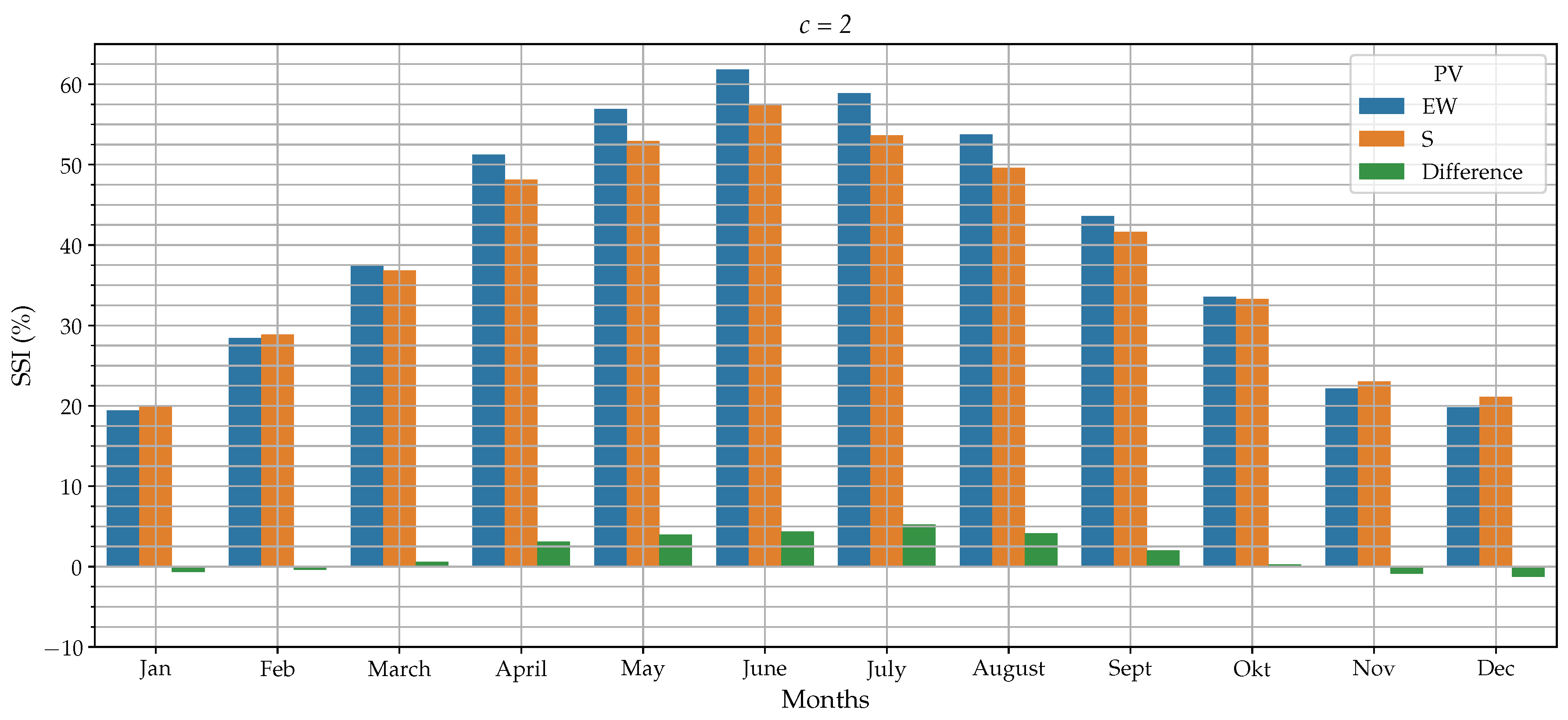
The limited increase of SSI can be further investigated by analyzing the SSI on a monthly basis in order to take the seasonal effects into consideration. Figure 9 shows the median SSI for east/west- and south-oriented PV and the differences between them using large consumer profiles. It is clear that the benefit is particularly present during the spring and summer months. During these months, the SSI increases up to 5 percent points compared to a south-oriented PV installation. This has two reasons:
- -
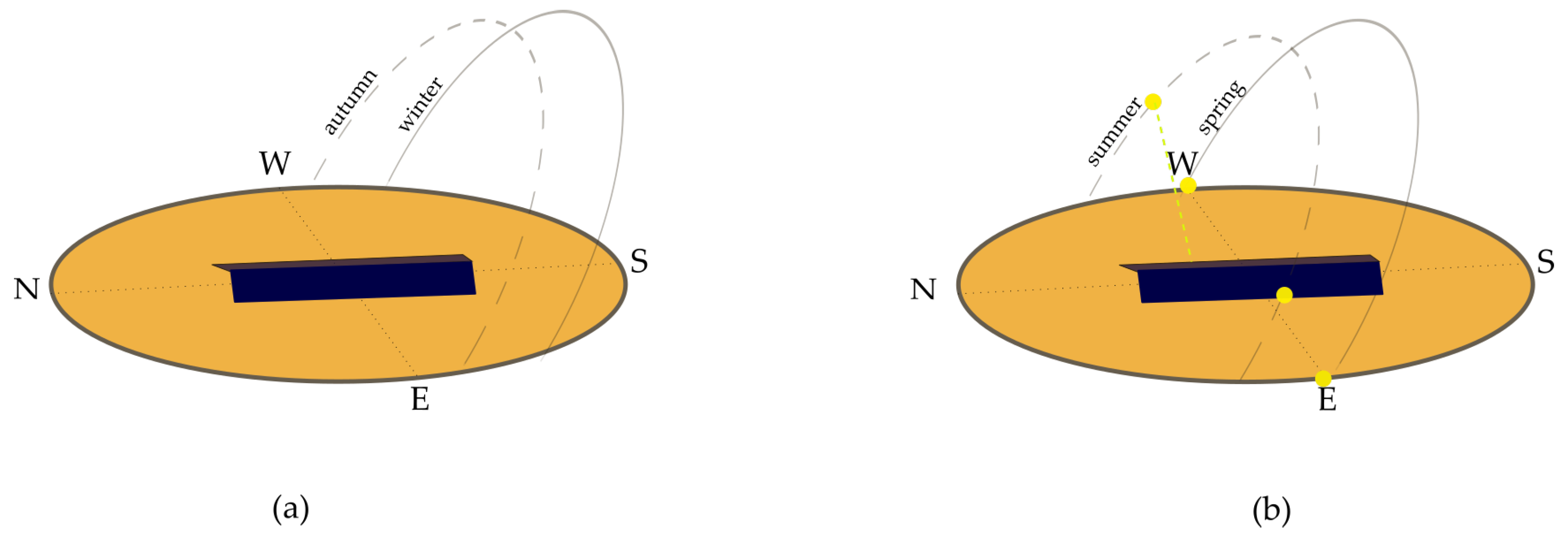
- In the northern hemisphere, the autumn and winter sun rises near the southeast and sets near the southwest. Hence, the direct irradiance is limited, while, during the spring and the summer, the sun rises near the east and northeast and sets near the west and northwest. Consequently, the yield increases during the morning and evening and reaches its maximum when the sun crosses the east and the west. The higher zenith angle of the sun during the spring, and especially during the autumn and the winter, causes the south facing panels to have a more optimal angle of incidence during a larger part of the day. This leads, according to Equation (6), to a higher direct irradiance. Figure 10 illustrates the solar trajectory during different seasons.
- -
- During the winter months, the winter solstice occurs. The earth’s poles are tilted away from the sun causing shorter daylight. Accordingly, during these months, a south-oriented PV installation is more interesting to cover the day consumption.
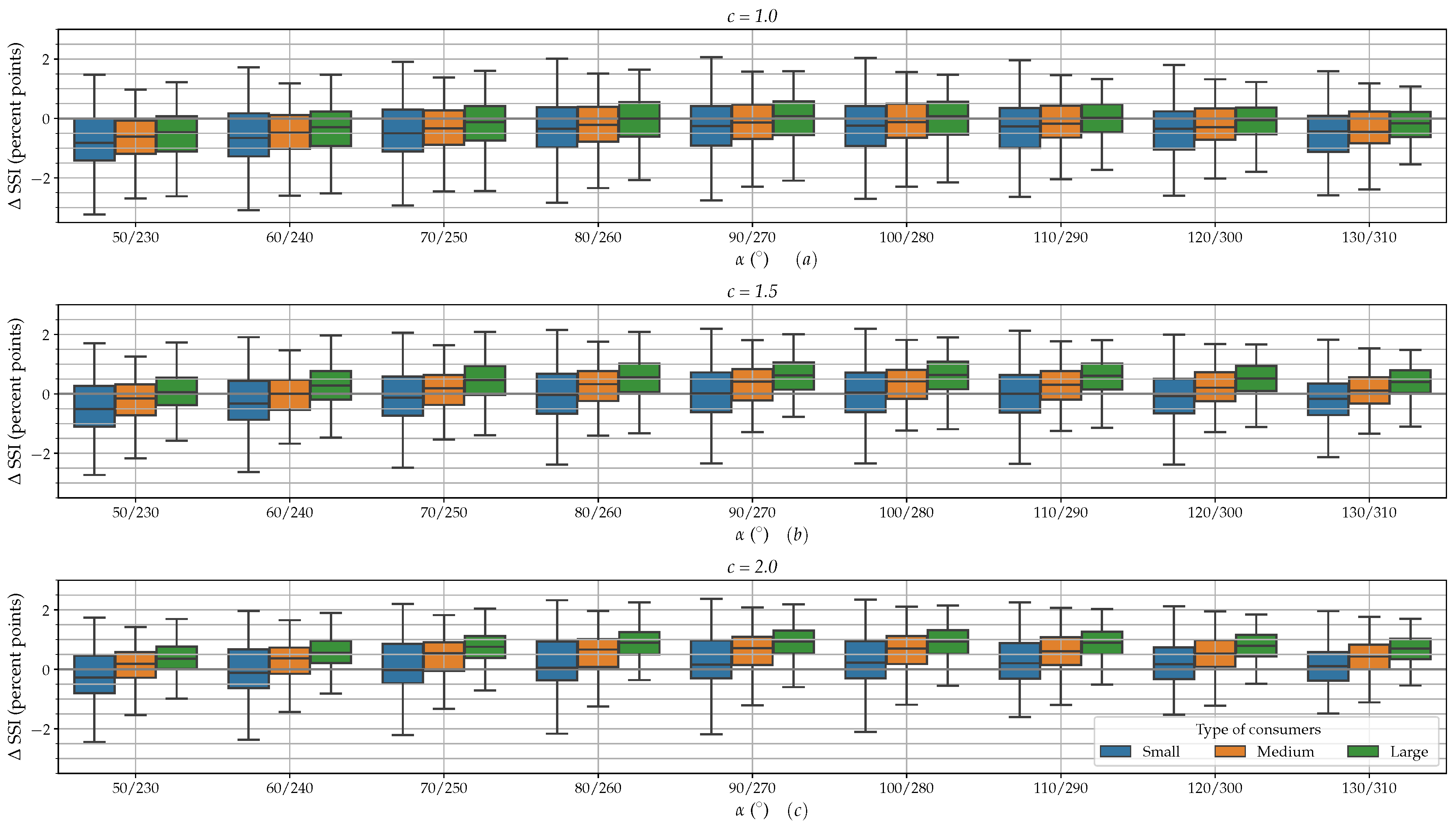
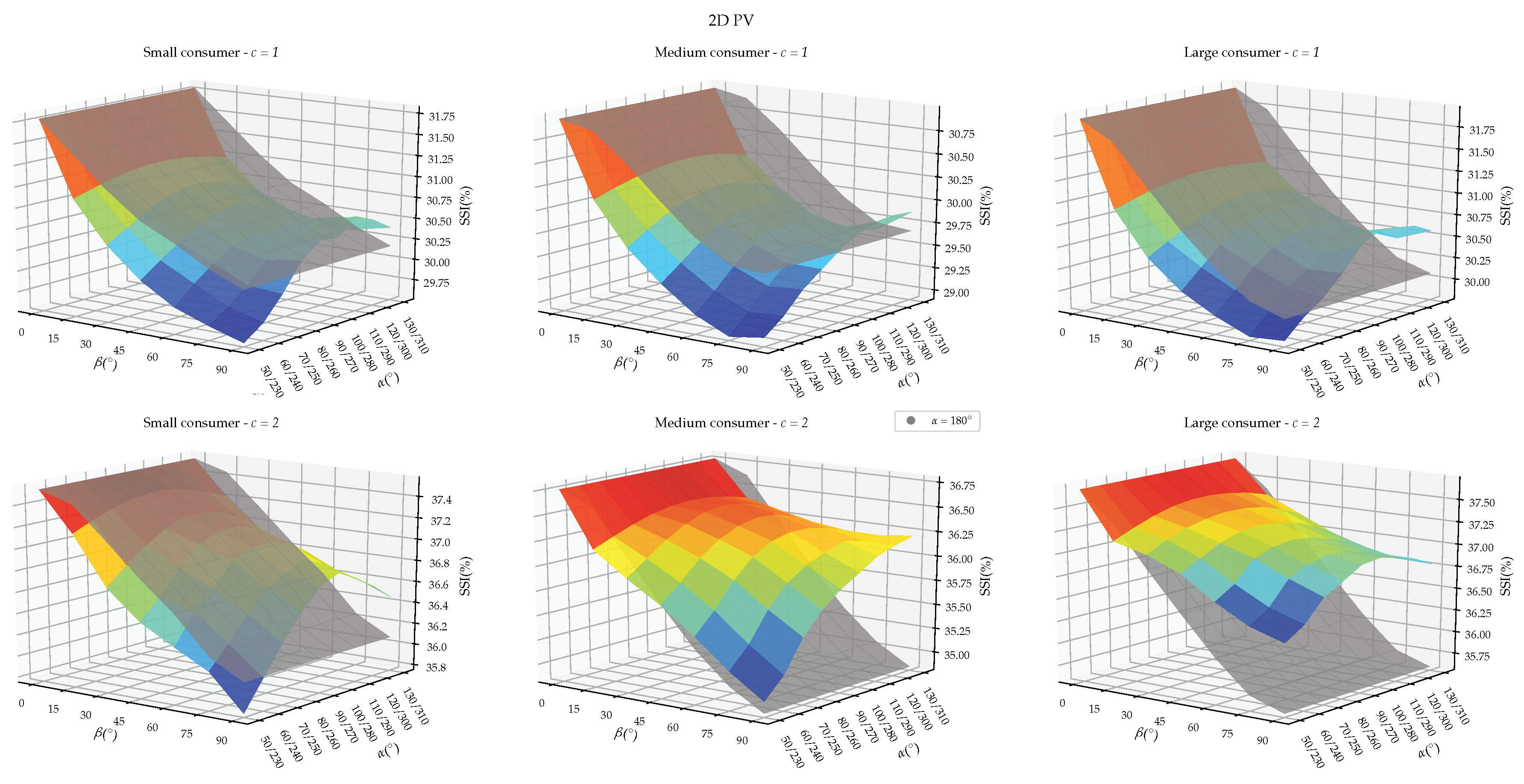
Until now, the analysis has been done by considering the median instead of the whole distribution. Moreover, only a number of specific azimuth angles have been investigated. In Figure 11, SSI is calculated for 2D PV installations following the methodology described in Section 2.6. The optimal azimuth angle with regard to the SSI is 90°/270°, irrespective of the type of consumer or the sizing factor. However, the large consumers can benefit more on SSI by orienting their PV installation to east/west than the small consumers. For , the median of SSI amounts to one percent point for large consumers and 0.2 percent points for small consumers with outliers going up to 2.4 percent points. For small consumers, the q25 percentile is negative, while, for other types of consumers, only the outliers are negative.
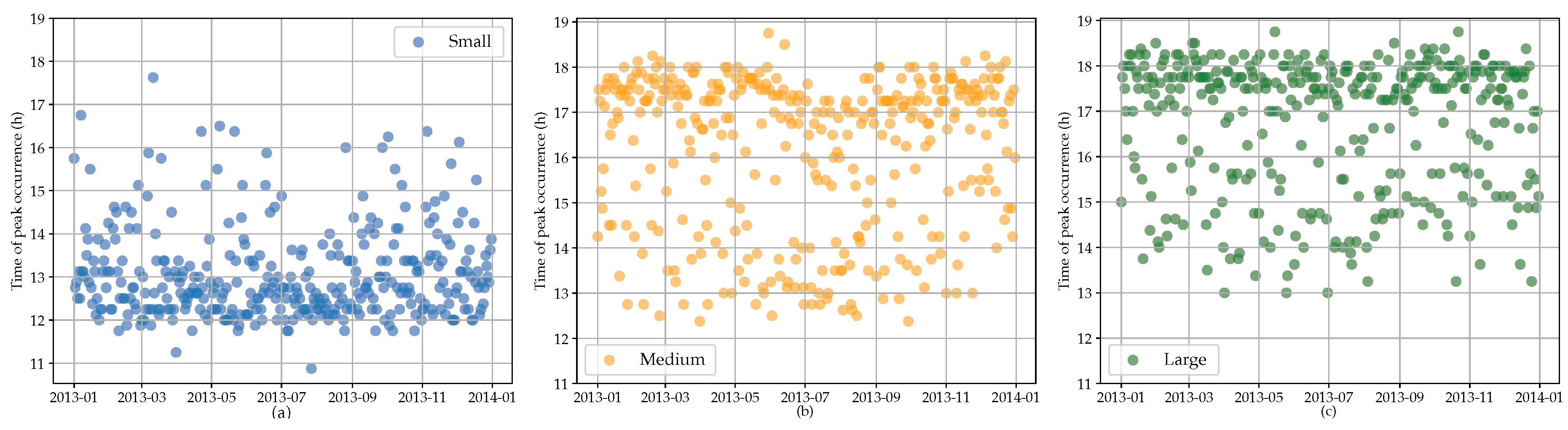
The distributional differences could be explained by analyzing the time of peak occurrence (ToP) of the different types of consumers. The result of this analysis is shown in Figure 12. Large and medium consumers usually have their peak demand during the evening while small consumers have their peak during the morning. The latter could be explained by the fact that those small consumers are possibly representing retired persons who generally have lower electricity consumption and are doing their activities especially during the middle of the day [45,46]. The spread of the ToP for medium consumers is larger than for large consumers. Moreover, only a slight difference can be noticed for the maximum ToP between medium and large consumers. They both have a maximal ToP between 17 h and 18 h. It should be noted that the outliers usually represent the weekends.
As the ToP of small consumers is usually at noon time but with a spread over the whole afternoon, SSI is small and also has a large spread. The median of SSI is slightly higher for large consumers compared to small consumers because of the slightly higher ToP and the smaller spread. Therefore, it can be concluded that east/west-oriented PV is more interesting for medium and especially for large consumers as they typically have a ToP occurring during evening.
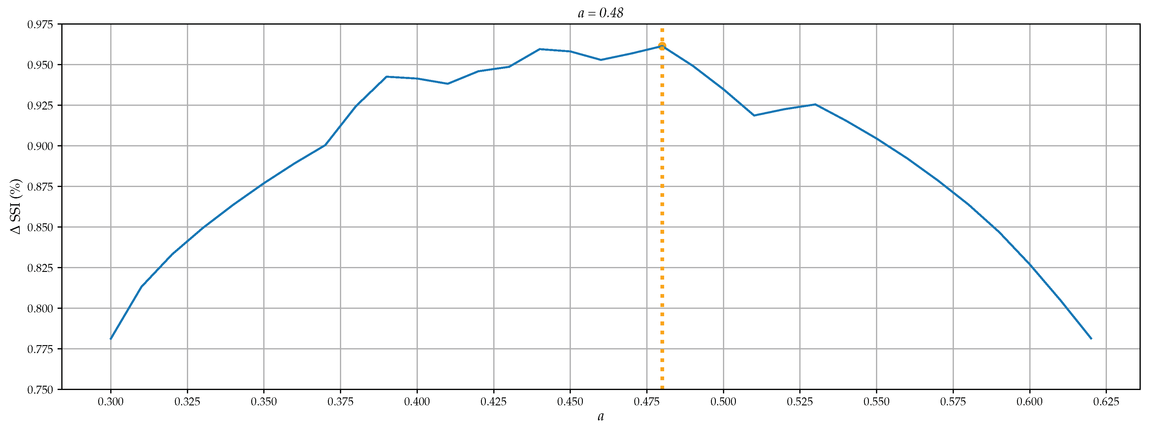
In the previous analysis for 2D PV, it is considered that the installed PV capacity is equal for both sides of the roof. From a practical viewpoint, this is not always possible due to e.g., shading obstacles or roof windows. Moreover, it is not yet proven that an equal spread of PV is the most optimal solution. Therefore, a sensitivity analysis is performed for SSI in a function of the parameter a for and for large consumers. The result of this analysis is shown in Figure 13. The curve shows that the maximal SSI is achieved for . This confirms that the previously made consideration leads to the optimal solution.
Until now, only tilt angles of 45° have been considered as they represent a large part of the residential consumers. In Figure 14, the impact of the tilt angle on the median of the SSI has been investigated for different orientations. For PV installations with , it has already been investigated that there is rather no benefit compared to a south oriented PV installation. However, for higher tilt angles of 75° or 90°, the benefit increases, especially for E/W- to SE/NW-oriented PV.
For PV installations with , the benefit is even more visible for high tilt angles, particularly for medium and large consumers. The optimal azimuth angle for small and large consumers is 90°/270° irrespective of the tilt angle, while, for medium consumers, the optimal orientation shifts to SE/NW as the tilt angle increases. In Table 5, it is shown that 1D PV installations oriented to the east or to the west, considering large consumers, are more strongly influenced by the tilt angle but are in any case not an improvement compared to south-oriented PV. It is remarkable that the SSI increases slightly once the tilt angle is 90°. Two results of this analysis are indicating the potential of building-integrated PV (BIPV). Firstly, the highest SSI could be achieved for (e.g., transparent solar panels as roof windows). Secondly, the highest benefit in SSI of E/W-oriented PV compared to south-oriented PV is for a vertically installed PV (e.g., facade integrated PV). The authors do suggest for future research to investigate more in detail the benefit of BIPV with regard to self-sufficiency.
3.2. Peak Reduction
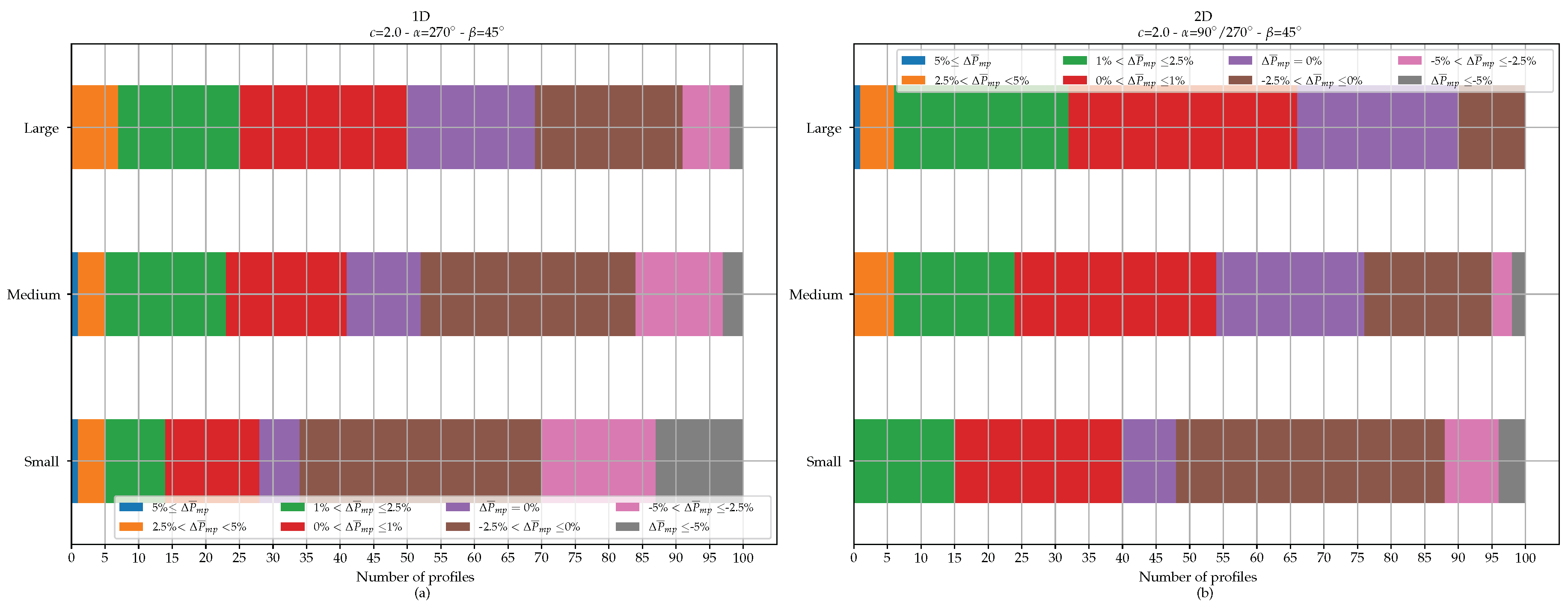
In this paragraph, the peak reduction due to oriented PV is assessed by calculating the moving average of the month peaks on an annual basis. Both 1D and 2D PV are considered and only PV systems with are considered as it is found that only for these sizing factors is a notable improvement achievable. The result of this analysis is shown in Figure 15. The bar graph can be interpreted as follows. The horizontal axis represents the number of profiles, the vertical axis represents the type of consumers, and the different colored stacks represent the benefit with regard to the moving average month peak.
For 1D configurations, the greatest benefit can be achieved with large consumers as they usually have their ToP in the evening. Almost 45% of the profiles can achieve a saving (which means ) on the peak load and nearly 7% can achieve a savings of more than 2.5%. At the same time, approximately 30% should pay more because of not covering the peak demand appropriately. This part increases further for medium and small consumers, due to the mismatch of the ToP and the PV production.
For east/west-oriented PV, higher benefits could be achieved. Again, this is especially the case for large consumers. More than 60% could achieving a saving in peak load while only 10% should pay more. Nearly 6% would save more than 2.5%. For medium and large consumers, the share of profiles achieving a saving is also higher than for 1D PV. Almost 50% of the medium consumers and 40% of the small consumers could achieve savings. East/west-oriented PV is thus more beneficial as it has a bigger chance to cover the month peak due to the spread yield during the day.
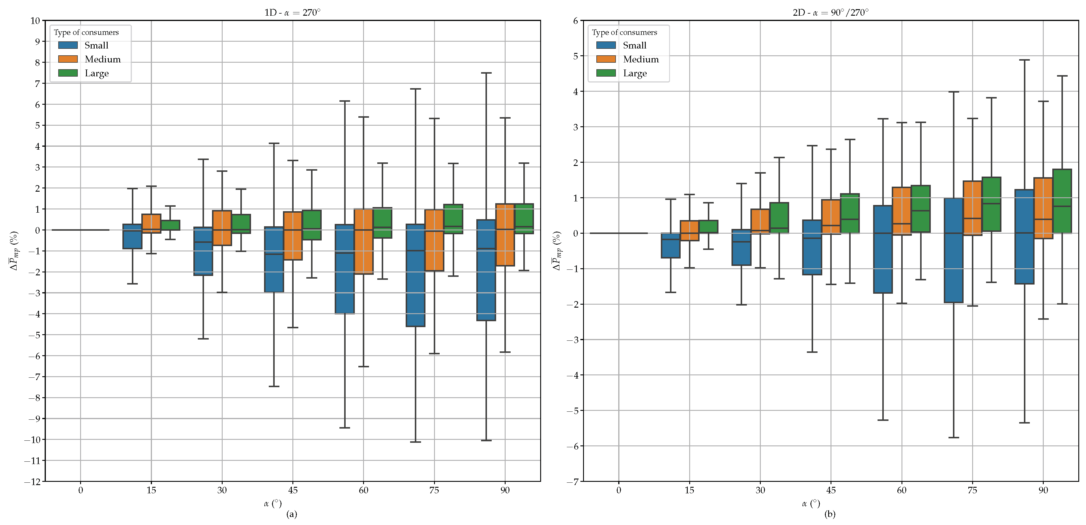
When looking at the impact of the tilt angle on Figure 16, it can be noticed that the spread increases with increasing tilt angle. This is both the case for west-oriented and east/west-oriented PV. However, for east/west-oriented PV, the median increases also while that is not really the case for west-oriented PV. This increase could be explained by the fact that a higher tilt angle causes the PV installations to produce until later in the evening. For , the median reduction amounts 0.73 percent points for 2D PV installations with outliers of 4.5 percent points. However, this analysis showed that neither the tilt angle nor the azimuth angle causes a significant reduction of the month peaks.
3.3. Storage
The benefit in terms of energy storage can be analyzed by calculating the needed storage capacity for a certain desired SSI and for the amount of installed PV. This is done for a south- and east/west-oriented PV installation with both the typical tilt angle and then compared to each other. The analysis is only performed with large consumer profiles as they basically achieve the highest SSI. It should be noted that the storage capacity is here considered as the usable storage capacity, thus excluding all the losses such as self-discharge and converter losses. As the aim of this analysis is to compare two results, these aspects are of little relevance. In order to determine the benefit, the ratio is defined as the ratio between the needed energy storage system capacity for an east/west-oriented PV installation and a south-oriented PV installation :
The result of this analysis is shown in Figure 17a in the form of a contour plot with on the horizontal axis the desired SSI; on the vertical axis, the installed PV capacity and the contours representing the ratio . For , an east/west-oriented PV installation will need a smaller storage capacity to achieve a certain SSI than when having the PV installation south-oriented. The isoline for is shown as a full black line. When observing the contourplot it can be noticed that a benefit is only achievable for PV installations with and for . When wanting to achieve for example a SSI of 60% and having a PV installation with , 10% of storage capacity could be saved due to orienting the PV to east/west. For higher SSI, east/west-oriented PV is not considered viable; due to lower yield during the winter, a very large storage system would be needed.
When considering residential storage systems, often electrochemical batteries, those savings are not in the order of magnitude to be considered as meaningful. Nevertheless, inversely it could be stated that, with the same storage capacity, the battery utilization could be reduced. This metric is expressed in discharge cycles per year and can be used to determine the expected end of lifetime. For this analysis, the comparison is done for an east/west- and south-oriented PV and the percentage of reduction of battery utilization is calculated as follows:
with the relative difference of the battery utilization and and , respectively, the discharge cycles for south-oriented and east/west-oriented PV. represents the discharged power at time t. Figure 17b shows the difference in battery utilization between east/west and south-oriented PV as a function of SSI and c. As can be seen, this difference is always positive, which means that, in any case, the battery utilization could be reduced. However, this is mainly due to the fact that, when a larger storage system is needed, it will be de facto underutilized during the summer. This underutilization is, as aforementioned, the consequence of the higher SSI of PV during the non-winter months, while during the winter the SSI is lower compared to a south-oriented PV installation (see also Figure 9). Therefore, only the results above the black line are relevant. This line represents the sizing factor c and the SSI for which the needed storage capacity is the same for east/west- and south-oriented PV, thus with . For the same operating point as given in the example above (, ), a reduction in battery utilization of 5% could be reached. For the isoline , a reduction of 6% is possible. It is obvious to state that this will lead to a slight extension of the battery lifetime. However, it should be noted that the cyclic lifetime depends on many other factors and parameters than just the battery utilization, such as cell temperature, depth of discharge, and charge/discharge rate. However, the number of discharge cycles determines to a large extent the cyclic lifetime of batteries [47].
3.4. General Overview
Table 6 shows an overview of the benefits and the drawbacks of east/west-oriented PV compared to south-oriented PV for and . For SSI, SCI, and the displayed results are the median of the distribution.
It should be noted that the results in the table are expressed in percent points as they represent absolute differences. For the annual yield and the PV peak power, it is assumed that, for a south-oriented PV installation, they both amount to 100%. As the SSI is lower for 1D PV, the benefit regarding the battery utilization is not investigated. The results SSI, SCI, and are already discussed in detail previously; below, some more explanation will be given on the other results:
- -
- Due to the non-optimal orientation, the annual yield () for west and east/west-oriented PV is approximately 24% less than for a south-oriented PV installation.
- -
- The maximum produced power is especially lower for an east/west-oriented PV installation. The reduction amounts almost 26.01% while for a west-oriented PV installation it amounts almost 4%. The lower peak power can create two benefits. The lower peak implies that the inverter can be sized smaller. Secondly, a smaller inverter leads to lower grid tariff for prosumers, at least in Flanders (Belgium), where this tariff is dependent on the AC-power of the inverter [48].
- -
- A last point concerns the injected energy. This could also be represented as the complement of the self-consumption. This is almost 6.5% lower for 2D PV and 4.5% for 1D PV. The lower the injected energy, the lower the grid load. Moreover, the new grid tariff structure proposed by the Flemish regulator (VREG) includes a tariff that is calculated pro rata the injected energy.
4. Conclusions
A number of publications addressed the benefit of orienting PV panels towards other directions than the south. However, the outcome of these studies differ from each other so that no firm conclusion can be taken. In this study, a large dataset of consumption profiles is used and conclusions are made according to the consumer class. Moreover, the in-plane irradiance is calculated by the Hay & Davies model which is the most appropriate transposition model for PV oriented to other directions than the south. This study included a complete analysis taking into account all the possible benefits for an individual residential consumer. The comparison between the SSI and SCI obtained by measured and calculated PV production profiles showed that the simulation model is able to accurately estimate those indexes. The sensitivity analysis of the SSI as a function of the size of the PV installation showed that only a slight increase of SSI is possible, but only for oversized PV installations. Furthermore, large consumers can reach a slightly higher SSI than medium and small consumers.
Other possible 2D configurations were investigated, but it is shown that the east/west-oriented PV is the most optimal configuration. When analyzing the SSI on a monthly basis, the increases are only noticeable during the spring and summer months. During these months, the sun rises near the east and northeast and sets near the west and northwest. Consequently, the amount of direct irradiance reaching the PV panel reaches its maximum when the sun crosses the east and the west. Secondly, due to the winter solstice, the days are shorter and a south-oriented PV installation is more interesting to cover the day consumption. Regarding 1D PV, east- and west-oriented PV have a much lower SSI, regardless of the size of the installation or the type of consumer.
The distributional differences of SSI between the type of consumers, with the large consumers having a higher median SSI than medium and small consumers, is related to the ToP occurrence of the demand. As small consumers usually have their peak demand during the noon, east/west-oriented PV is not very interesting for them. On the other hand, medium and especially large consumers have their peak clearly in the evening, thus this leads to a slightly higher SSI. Regarding the SCI, very significant increases are noticeable especially for east/west-oriented PV. However, this is not due to a better match between demand and production but rather due to the lower production. Hence, the surplus of energy injected to the grid is lower causing a lower impact on the distribution grid and in some countries as Belgium. This leads to lower grid tariffs.
The sensitivity analysis of SSI in function of the tilt angle showed that the highest SSI could be achieved for horizontal PV. The highest benefit of east/west-oriented PV compared to south-oriented PV is found to be for vertical PV. This proves that BIPV has potential when it comes to increasing self-sufficency. The optimal azimuth angle for small and large consumers is 90°/270° irrespective of the tilt angle while, for medium consumers, the optimal orientations shift to SE/NW as the tilt angle increases.
The peak reduction is investigated by calculating the moving average of the month peaks cfr. The tariff methodology proposed by the VREG. For 1D and 2D PV, 6 to 7% of the large consumers could reach savings between 2.5% and 5%. For 50% of the large consumers that has a PV installation facing the west, savings are possible while, for large consumers, this percentage amounts to 67%. These values decrease for medium and small consumers which shows that, as for the SSI, the benefit is especially present for large consumers. The tilt angle has only a slight effect on the peak reduction for 2D PV installations with large consumers causing a larger spread and an increase of the median with almost 0.75 percent points. Regarding storage capacity, savings are possible when largely oversizing the PV installation and aiming for a reasonable SSI (<70%). However, when considering residential storage systems, those savings cannot be considered as meaningful. For that reason, the battery utilization has also been investigated. It was found that the annual discharge cycles decrease with 6% when having an east/west-oriented PV installation.
This study showed that an east/west-oriented PV installation has many benefits, but many of these benefits are not very significant (see Table 6). However, these benefits are particularly apparent with large consumers and oversized PV installations. The slight increase of the SSI means that the energy purchased from the grid will slightly decrease. At the same time, the amount of injected energy decreases considerably which means that the grid injection costs will reduce. Furthermore, the PV peak power reduces by almost 26%, which means that a smaller inverter is needed and so the prosumer tariff will decrease. Lastly, the reduction of the average month peak is marginal and the utilization of the battery decreases slightly. In short, these are all slight benefits, but the sum of them could make an east/west-oriented PV more interesting in terms of investment and electricity cost. A suggestion for further research is to translate these benefits into economic terms taking into account all the operating and capital expenditures (OPEX and CAPEX).
This article focused on the benefits for an individual residential consumer with the possibility to install PV at one or two roof sides considering the same tilt angle. However, as energy communities are nowadays gaining more and more attention, sharing PV energy within the community will be evident in the near future. By aggregating distributed energy resources, the affordability could be increased and a higher SCI could be achieved [49,50]. Moreover, on the community level, the orientation and inclination could be optimized in a more flexible way such that a higher benefit could be obtained. This optimization problem will be tackled in a second publication.
Author Contributions
Conceptualization, H.A. and J.D.; methodology, H.A. and J.D.; software, H.A.; validation, H.A.; formal analysis, H.A.; investigation, H.A. and J.D.; resources, J.D.; data curation, J.D.; writing—original draft preparation, H.A.; writing—review and editing, H.A., J.D., and L.V.; visualization, H.A.; supervision, J.D. and L.V.; project administration, J.D. and L.V.; funding acquisition, J.D. and L.V. All authors have read and agreed to the published version of the manuscript.
Funding
This publication frames within the EMPOWER2.0 project, which receives financial support from the European Fund for Regional Development via the Interreg North Sea Region Program. The sole responsibility for the content of this publication lies with the authors. It does not necessarily reflect the opinion of the European Union. Neither the Interreg North Sea Region Programme nor the European Commission are responsible for any use that may be made of the information contained therein. More information is available at: https://northsearegion.eu/empower-20/.
Acknowledgments
The authors would like to thank the Flemish distribution system operator Fluvius for providing the dataset of consumption profiles. Secondly, the authors would also like to thank the RMI for providing the meteorological data that have been used as input for the calculation of the irradiance and the PV system model.
Conflicts of Interest
The authors declare no conflict of interest.
References
- European Commission. National Energy and Climate Plans 2020 (NECPs). Available online: https://ec.europa.eu/info/energy-climate-change-environment/overall-targets/national-energy-and-climate-plans-necps_en (accessed on 1 August 2020).
- IEA. Global CO2 Emissions in 2019. Available online: https://www.iea.org/articles/global-co2-emissions-in-2019 (accessed on 1 August 2020).
- Schmela, M. Global Market Outlook For Solar Power: 2019–2023; SolarPower Europe Brussels: Brussels, Belgium, 2018; pp. 8–26. [Google Scholar]
- Kato, T. Record Efficiency for Thin-Film Polycrystalline Solar Cells up to 22.9% Achieved by Cs-Treated Cu(In,Ga)(Se,S)2. IEEE Photovolt. 2019, 9, 325–331. [Google Scholar] [CrossRef]
- Taguchi, M. 24.7% Record Efficiency HIT Solar Cell on Thin Silicon Wafer. IEEE Photovolt. 2014, 10, 96–100. [Google Scholar] [CrossRef]
- IEA. Task1: Strategic PV Analysis and Outreach. In Snapshot of Global PV Markets 2020; Masson, G., Ed.; IEA: Paris, France, 2020; pp. 10–15. [Google Scholar]
- Axaopoulos, P.J. Energy and Economic Comparative Study of a Tracking vs a Fixed Photovoltaic System in the Northern Hemisphere. Nova Energy Environ. Econ. 2013, 21, 1–20. [Google Scholar]
- Hersch, P.; Zweibel, K. Basic Photovoltaic Principles and Methods; Bird, R., Ed.; Technical Information Office: Springfield, CA, USA, 1982; pp. 5–8.
- Jacobson, M.Z.; Jadhav, V. World estimates of PV optimal tilt angles and ratios of sunlight incident upon tilted and tracked PV panels relative to horizontal panels. Sol. Energy 2018, 169, 55–66. [Google Scholar] [CrossRef]
- Soulayman, S. Optimal Tilt Angle and Maximum Possible Solar Energy Gain at High Latitude Zone. Sol. Energy Res. 2016, 12, 25–35. [Google Scholar]
- Wirth, H. Recent Facts about Photovoltaics in Germany; Fraunhofer Institute for Solar Energy Systems ISE: Freiburg, Germany, 2020; Available online: https://www.ise.fraunhofer.de/content/dam/ise/en/documents/publications/studies/recent-facts-about-photovoltaics-in-germany.pdf (accessed on 3 August 2020).
- European Commission. State Aid: Commission Endorses Three French Initiatives to Produce More Than 17 Gigawatts in Renewable Energy. Available online: https://ec.europa.eu/commission/presscorner/detail/en/IP_17_1231 (accessed on 3 August 2020).
- Solar Guide. Smart Export Guarantee to Replace FiT from 2020. Available online: https://www.solarguide.co.uk/smart-export-guarantee-replace-fit#/ (accessed on 3 August 2020).
- Ofgem. Feed-In Tariff (FIT) Rates. Available online: https://www.ofgem.gov.uk/environmental-programmes/fit/fit-tariff-rates (accessed on 3 August 2020).
- VREG. De Digitale Meter bij Zonnepaneleneigenaars. Available online: https://www.vreg.be/nl/de-digitale-meter-bij-zonnepaneleneigenaars (accessed on 3 August 2020).
- VEA. Persbericht: Vlaanderen Blijft Inzetten op Zonne-Energie. Available online: https://www.energiesparen.be/nieuws/persbericht/vlaanderen-blijft-inzetten-op-zonne-energie (accessed on 3 August 2020).
- Van Ryckeghem, J.; Delerue, T.; Bottenberg, A.; Rens, J.; Desmet, J. Decongestion of the distribution grid via optimised location of PV-battery systems. Conf. PQ EMC 2017, 24, 573–577. [Google Scholar] [CrossRef] [Green Version]
- Weniger, J.; Tjaden, T.; Quaschning, V. Sizing of residential PV battery systems. Energy Procedia 2014, 46, 78–87. [Google Scholar] [CrossRef] [Green Version]
- Lahnaoui, A.; Stenzel, P.; Linssen, J. Tilt angle and orientation impact on the techno-economic performance of photovoltaic battery systems. Energy Procedia 2017, 105, 4312–4321. [Google Scholar] [CrossRef]
- Mubarak, R.; Luiz, E.W.; Seckmeyer, G. Why PV Modules Should Preferably No Longer Be Oriented to the South in the Near Future. Energies 2019, 12, 4528. [Google Scholar] [CrossRef] [Green Version]
- Laveyne, J.I.; Bolazakov, D.; Van Eetvelde, G.; Vandevelde, L. Impact of Solar Panel Orientation on the Integration of Solar Energy in Low-Voltage Distribution Grids. J. Photoenergy 2020. [Google Scholar] [CrossRef]
- Perez, R.; Ineichen, P.; Seals, R.; Michalsky, J.; Stewart, R. Modeling daylight availability and irradiance components from direct and global irradiance. Sol. Energy 1990, 44, 271–289. [Google Scholar] [CrossRef] [Green Version]
- Klucher, T.M. Evaluation of models to predict insolation on tilted surfaces. Sol. Energy 1990, 23, 111–114. [Google Scholar] [CrossRef]
- Reindl, D.T.; Beckman, W.A.; Duffie, J.A. Evaluation of hourly tilted surface radiation models. Sol. Energy 1990, 45, 9–17. [Google Scholar] [CrossRef]
- Davies, J.A.; Hay, J.E. Calculation of the solar radiation incident on an inclined surface. In Proceedings of the 1st Canadian Solar Radiation Data Workshop, Toronto, ON, Canada, 17–19 April 1978; pp. 59–72. [Google Scholar]
- Eurostat. Energy Statistics-Electricity Prices for Domestic and Industrial Consumers, Price Components. Available online: https://ec.europa.eu/eurostat/cache/metadata/en/nrg_pc_204_esms.htm (accessed on 3 August 2020).
- Consortium of AF-Mercados, REF-E and Indra. Final Report: Study on Tariff Design for Distribution Systems. Available online: https://ec.europa.eu/energy/sites/ener/files/documents/20150313%20Tariff%20report%20fina_revREF-E.PDF (accessed on 3 August 2020).
- VREG. Tariefmethodologie Voor Distributie Elektriciteit en Aardgas Gedurende de Reguleringsperiode 2021–2024. Available online: https://www.vreg.be/sites/default/files/Tariefmethodologie/2021-2024/tariefmethodologie_reguleringsperiode_2021-2024.pdf (accessed on 3 August 2020).
- Liu, B.; Jordan, R. Daily insolation on surfaces tilted towards equator. ASHRAE 1961, 10, 526–541. [Google Scholar]
- Demain, C.; Journée, M.; Bertrand, C. Evaluation of different models to estimate the global solar radiation on inclined surfaces. Renew. Energy 2013, 50, 710–721. [Google Scholar] [CrossRef]
- Maleki, S.A.M.; Hizam, H.; Gomes, C. Estimation of Hourly, Daily and Monthly Global Solar Radiation on Inclined Surfaces: Models Re-Visited. Energies 2017, 10, 134. [Google Scholar] [CrossRef] [Green Version]
- Nikiforiadis, N. Modeling Solar Irradiance; School of Science & Technology: Thesaaloniki, Greece, 2014. [Google Scholar]
- Mubarak, R.; Hofmann, M.; Riechelmann, S.; Seckmeyer, G. Comparison of Modelled and Measured Tilted Solar Irradiance for Photovoltaic Applications. Energies 2017, 11, 1688. [Google Scholar] [CrossRef] [Green Version]
- Spencer, J.W. Fourier series representation of the sun. Search 1971, 2, 172. [Google Scholar]
- Reno, M.J.; Hansen, C.W.; Stein, J.S. Global Horizontal Irradiance Clear Sky Models: Implementation and Analysis; Sandia National Laboratories, U.S. Department of Energy: Oak Ridge, TN, USA, 2007. Available online: https://prod-ng.sandia.gov/techlib-noauth/access-control.cgi/2012/122389.pdf (accessed on 5 August 2020).
- Holm, W.F.; Clifford, W.H.; Mikofski, M.A. pvlib python: A python package for modeling solar energy systems. Open Source Softw. 2018, 3, 884. [Google Scholar]
- King, D.L.; Boyson, W.E.; Kratochvill, J.A. Photovoltaic Array Performance Model; Sandia National Laboratories, U.S. Department of Energy: Oak Ridge, TN, USA, 2004. Available online: https://prod-ng.sandia.gov/techlib-noauth/access-control.cgi/2004/043535.pdf (accessed on 6 August 2020).
- King, D.L.; Gonzalez, S.; Galbraith, G.M.; Boyson, W.E. Performance Model for Grid-Connected Photovoltaic Inverters; Sandia National Laboratories, U.S. Department of Energy: Oak Ridge, TN, USA, 2007. Available online: https://citeseerx.ist.psu.edu/viewdoc/download?doi=10.1.1.464.6452&rep=rep1&type=pdf (accessed on 6 August 2020).
- Mondol, J.D.; Yohanis, Y.G.; Norton, B. The impact of array inclination and orientation on the performance of a grid-connected photovoltaic system. Renew. Energy 2007, 32, 118–140. [Google Scholar] [CrossRef]
- Mondol, J.D.; Yohanis, Y.G.; Norton, B. Optimal sizing of array and inverter for grid-connected photovoltaic systems. Sol. Energy 2006, 80, 1517–1539. [Google Scholar] [CrossRef]
- PVOutput Dataset. Available online: https://pvoutput.org/ (accessed on 15 January 2019).
- Beck, T.; Kondziella, H.; Huard, G.; Bruckner, T. Assessing the influence of the temporal resolution of electrical load and PV generation profiles on self-consumption and sizing of PV-battery systems. Appl. Energy 2016, 173, 331–342. [Google Scholar] [CrossRef]
- Ried, S.; Jochem, P.; Fichtner, W. Profitability of Photovoltaic Battery Systems Considering Temporal Resolution. In Proceedings of the 2015 12th International Conference on the European Energy Market (EEM), Lisbon, Portugal, 19–22 May 2015. [Google Scholar]
- Bertrand, C.; Housmans, C.; Leloux, J. Solar Irradiation from the Energy Production of Residential PV Systems (Spider); RMI: Brussels, Belgium, 2017; Available online: https://www.belspo.be/belspo/brain-be/projects/FinalReports/SPIDER_FinRep.pdf (accessed on 1 August 2020).
- Wyatt, P. A dwelling-level investigation into the physical and socio-economicdrivers of domestic energy consumption in England. Energy Policy 2013, 60, 540–549. [Google Scholar] [CrossRef]
- Anderson, B.; Torriti, J. Explaining shifts in UK electricity demand using time use data from 1974 to 2014. Energy Policy 2018, 123, 544–557. [Google Scholar] [CrossRef]
- Sarasketa-Zabala, E.; Martinez-Laserna, E.; Berecibar, M.; Gandiaga, I.; Rodriguez-Martinez, L.M.; Villarreal, I. Realistic lifetime prediction approach for Li-ion batteries. Appl. Energy 2016, 162, 839–852. [Google Scholar] [CrossRef]
- VREG. Prosumententarief 2020. Available online: https://www.vreg.be/nl/prosumententarief-2020 (accessed on 13 August 2020).
- Jones, K.B.; Benett, E.C.; Ji, F.W.; Kazerooni, B. Beyond Community Solar: Aggregating Local Distributed Resources for Resilience and Sustainability. In How Distributed Energy Resources are Disrupting the Utility Business Model; Sioshansi, F.P., Ed.; Menlo Energy Economics: Walnut Creek, CA, USA, 2017; pp. 65–81. [Google Scholar]
- Noll, D.; Dawes, C.; Varun, R. Solar Community Organizations and active peer effects in the adoption of residential PV. Energy Policy 2014, 67, 330–343. [Google Scholar] [CrossRef]
Figure 1.
Inverter efficiency curve.

Figure 2.
Distribution of the annual consumption for the different consumption classes.

Figure 3.
Annual PV production as a function of the orientation and sizing factor c.

Figure 4.
Effect of the temporal resolution on the: (a) RE for direct consumed PV energy and (b) on the SSI and SCI distribution.
Figure 4.
Effect of the temporal resolution on the: (a) RE for direct consumed PV energy and (b) on the SSI and SCI distribution.

Figure 5.
Illustration of SSI and SCI with calculated PV profiles for: a day in the (a) spring, (b) the summer, and (c) the autumn.
Figure 5.
Illustration of SSI and SCI with calculated PV profiles for: a day in the (a) spring, (b) the summer, and (c) the autumn.

Figure 6.
Directions and tilt angle of the PV installation: (a) Illustration of a 2D and 1D PV installation; (b) azimuth angles considered for 2D PV installations.
Figure 6.
Directions and tilt angle of the PV installation: (a) Illustration of a 2D and 1D PV installation; (b) azimuth angles considered for 2D PV installations.

Figure 7.
Comparison of SCI and SSI with simulated and measured PV production profiles.

Figure 8.
Sensitivity analysis of SCI and SSI in function of c for different orientations by using: (a) small, (b) medium, and (c) large consumer profiles.
Figure 8.
Sensitivity analysis of SCI and SSI in function of c for different orientations by using: (a) small, (b) medium, and (c) large consumer profiles.


Figure 9.
Monthly SSI for east/west- and south-oriented PV installations and with .

Figure 10.
Trajectory of the sun during: (a) autumn and winter; (b) and during spring and summer.

Figure 11.
Distribution of SSI for different azimuth angles and with: (a) ; (b) ; (c) .

Figure 12.
Time of peak occurrence for: (a) small; (b) medium; (c) large consumers.

Figure 13.
Sensitivity analysis of the distribution of PV over the two roof sides in function of SSI for .
Figure 13.
Sensitivity analysis of the distribution of PV over the two roof sides in function of SSI for .

Figure 14.
SSI in function of the tilt and azimuth angle for small, medium, and large consumers for PV installations with and . SSI for 2D PV for different is shown in scaled colors and the south-oriented PV is shown in gray.
Figure 14.
SSI in function of the tilt and azimuth angle for small, medium, and large consumers for PV installations with and . SSI for 2D PV for different is shown in scaled colors and the south-oriented PV is shown in gray.

Figure 15.
Percentage of profiles having benefit of oriented PV with regard to the moving average of the month peaks for: (a) 1D PV; (b) 2D PV.
Figure 15.
Percentage of profiles having benefit of oriented PV with regard to the moving average of the month peaks for: (a) 1D PV; (b) 2D PV.

Figure 16.
Increase or decrease of the annual moving average of the month peaks for: (a) 1D PV installations; (b) 2D PV installations.
Figure 16.
Increase or decrease of the annual moving average of the month peaks for: (a) 1D PV installations; (b) 2D PV installations.

Figure 17.
lBenefit in terms of: (a) storage capacity; (b) battery utilization for east/west-oriented PV compared to south-oriented PV.
Figure 17.
lBenefit in terms of: (a) storage capacity; (b) battery utilization for east/west-oriented PV compared to south-oriented PV.


Table 1.
PV module type.
| Parameter | Module |
|---|---|
| Type | Sunpower SPR-230-WHT-U |
| Technology | Mono-Si |
| Peak Power | 230 W |
Table 2.
Parameters of the measured PV installations.
| Installation | A | B | C |
|---|---|---|---|
| 90° | 180° | 270° | |
| 45° | 45° | 45° | |
| 7590 W | 5750 W | 5060 W | |
| PV technology | Poly-si | Poly-si | Poly-si |
| Module type | Atersa A-230P | BS-250P | Mage Solar 230/6PJ |
| 6300 W | 215 W | 5060 W | |
| Inverter type | SMA SMC6000A | Enphase M215 | SMA SB 5000TL-20 |
Table 3.
q25, q50 and q75 values of SCI and SSI for measured and simulated PV production.
| Installation (Orientation) | A (E) | B (S) | |||||
| Percentile | q25 | q50 | q75 | q25 | q50 | q75 | |
| SCI (%) | Measured | 33.64 | 36.06 | 38.11 | 29.07 | 31.63 | 33.55 |
| Simulated | 33.67 | 35.93 | 38.03 | 29.44 | 31.89 | 33.74 | |
| SSI (%) | Measured | 26.73 | 28.65 | 30.28 | 29.07 | 31.63 | 33.55 |
| Simulated | 26.75 | 28.54 | 30.22 | 29.44 | 31.89 | 33.74 | |
| Installation (Orientation) | C (W) | A+C (E/W) | |||||
| Percentile | q25 | q50 | q75 | q25 | q50 | q75 | |
| SCI (%) | Measured | 35.04 | 38.22 | 40.18 | 37.43 | 40.25 | 42.79 |
| Simulated | 34.41 | 37.82 | 39.57 | 37.99 | 40.55 | 43.46 | |
| SSI (%) | Measured | 26.73 | 29.15 | 30.65 | 29.14 | 31.34 | 33.32 |
| Simulated | 26.25 | 28.84 | 30.18 | 29.58 | 31.58 | 33.84 | |
Table 4.
Benefit of SSI (%) for east/west-oriented PV for small, medium, and large consumers.
| SSI (%) | c | 0.5 | 1 | 1.5 | 2 |
|---|---|---|---|---|---|
| Small consumers | S | 23.91 | 30.77 | 34.62 | 36.86 |
| E/W | 23.13 | 30.63 | 34.61 | 37.11 | |
| [points] | −0.78 | −0.14 | −0.01 | 0.25 | |
| Medium consumers | S | 23.55 | 30.25 | 33.64 | 35.77 |
| E/W | 22.81 | 29.92 | 33.80 | 36.36 | |
| [points] | −0.75 | −0.33 | 0.16 | 0.59 | |
| Large consumers | S | 24.01 | 30.87 | 34.43 | 36.50 |
| E/W | 23.00 | 30.79 | 34.93 | 37.26 | |
| [points] | −1.01 | −0.07 | 0.50 | 0.76 |
Table 5.
SSI for east, west, east/west, and south facing PV installations with and for large consumers.
Table 5.
SSI for east, west, east/west, and south facing PV installations with and for large consumers.
| SSI (%) | ||||||||
|---|---|---|---|---|---|---|---|---|
| c | 1 | 2 | ||||||
| 90° | 270° | 90°/270° | 180° | 90° | 270° | 90°/270° | 180° | |
| 0° | 31.94 | 31.94 | 31.94 | 31.94 | 37.71 | 37.71 | 37.71 | 37.71 |
| 15° | 29.74 | 30.56 | 31.17 | 31.73 | 35.85 | 36.69 | 37.46 | 37.40 |
| 30° | 27.98 | 29.08 | 30.90 | 31.28 | 34.30 | 35.73 | 37.36 | 36.93 |
| 45° | 26.82 | 28.09 | 30.79 | 30.87 | 33.20 | 34.51 | 37.26 | 36.50 |
| 60° | 26.19 | 27.47 | 30.64 | 30.50 | 32.69 | 33.94 | 37.16 | 36.08 |
| 75° | 25.97 | 27.28 | 30.50 | 30.20 | 32.38 | 33.80 | 37.03 | 35.73 |
| 90° | 26.33 | 27.55 | 30.63 | 30.07 | 32.51 | 34.03 | 36.98 | 35.60 |
Table 6.
General overview of the benefit analysis of east/west-oriented PV compared to south-oriented PV.
Table 6.
General overview of the benefit analysis of east/west-oriented PV compared to south-oriented PV.
| (Percent Points) | 1D | 2D |
|---|---|---|
| 270° | 90°/270° | |
| −23.98 | −24.41 | |
| SSI | −1.72 | 0.94 |
| SCI | 4.59 | 6.46 |
| −0.06 | −0.39 | |
| −4.84 | −26.01 | |
| - | −6.16 |
© 2020 by the authors. Licensee MDPI, Basel, Switzerland. This article is an open access article distributed under the terms and conditions of the Creative Commons Attribution (CC BY) license (http://creativecommons.org/licenses/by/4.0/).
Share and Cite
MDPI and ACS Style
Azaioud, H.; Desmet, J.; Vandevelde, L. Benefit Evaluation of PV Orientation for Individual Residential Consumers. Energies 2020, 13, 5122. https://0-doi-org.brum.beds.ac.uk/10.3390/en13195122
AMA Style
Azaioud H, Desmet J, Vandevelde L. Benefit Evaluation of PV Orientation for Individual Residential Consumers. Energies. 2020; 13(19):5122. https://0-doi-org.brum.beds.ac.uk/10.3390/en13195122
Chicago/Turabian StyleAzaioud, Hakim, Jan Desmet, and Lieven Vandevelde. 2020. "Benefit Evaluation of PV Orientation for Individual Residential Consumers" Energies 13, no. 19: 5122. https://0-doi-org.brum.beds.ac.uk/10.3390/en13195122
Note that from the first issue of 2016, this journal uses article numbers instead of page numbers. See further details here.