Micro Nuclear Reactors: Potential Replacements for Diesel Gensets within Micro Energy Grids


1
Faculty of Energy Systems and Nuclear Science, Ontario Tech University (UOIT), Oshawa, ON L1G 0C5, Canada
2
Faculty of Engineering and Applied Science, Ontario Tech University (UOIT), Oshawa, ON L1G 0C5, Canada
*
Author to whom correspondence should be addressed.
Energies 2020, 13(19), 5172; https://0-doi-org.brum.beds.ac.uk/10.3390/en13195172
Submission received: 11 September 2020
/
Revised: 27 September 2020
/
Accepted: 30 September 2020
/
Published: 5 October 2020
(This article belongs to the Special Issue Nuclear Power, including Fission and Fusion Technologies 2021)
Abstract
:Resilient operation of medium/large scale off-grid energy systems, which is a key challenge for energy crisis solutions, requires continuous and sustainable energy resources. Conventionally, micro energy grids (MEGs) are adopted to supply electricity and thermal energy simultaneously. Fossil-fired gensets, such as diesel generators, are indispensable components for off-grid MEGs due to the intermittent nature of renewable energy sources (RESs). However, fossil-fired gensets emit a significant amount of greenhouse gases (GHGs). Therefore, this study investigates an alternative source as an economical and environmental replacement for diesel gensets that can reduce GHG emissions and ensure system reliability. A MEG is developed in this paper to support a considerably large-scale electric and thermal demand at Ontario Tech University (UOIT). Different sizes of diesel gensets and RESs, such as solar, wind, hydro, and biomass, are combined in the MEG for off-grid applications. To evaluate diesel gensets’ competency, the diesel genset is substituted by an emission-free generation source named microreactor (MR). The fossil-fired MEG and MR-based MEG are optimized by an intelligent optimization technique, namely particle swarm optimization (PSO). The objective of the PSO is to minimize the net present cost (NPC). The simulation results show that MR-based MEG could be an excellent replacement for a diesel genset in terms of NPC and selected key performance indicators (KPIs). A comprehensive sensitivity analysis is also carried out to validate the simulation results.
1. Introduction
Humanity’s desire for electric energy is expanding continuously with industrialization and global population growth. Around fifty percent of our total energy comes from burning fossil fuels. Still, 1.2 billion or more people around the world do not have access to modern energy supplies. People are adopting renewable energy sources (RESs) to accomplish their energy needs. However, it is reported that the intermittent nature of RESs has an adverse impact on the energy network. Therefore, the high penetration of RESs in the energy hub is inappropriate and challenging [1].
The world is currently searching for sustainable energy resources to satisfy today’s energy market. The energy resources that satisfy the present demand without compromising the future generation capability are regarded as sustainable energy sources. The term sustainable energy is often used interchangeably with green energy or renewable energy [2]. Therefore, RESs, such as wind, solar, hydropower, geothermal, and ocean energy, are identified as sustainable energy generation sources. Due to the intermittency of RESs, they can hardly provide a continuous electricity supply. Hence, alternative energy sources are required, which can act as a critical load or baseload supplier during RESs unavailability.
Affordable, resilient, and carbon-free electricity generation is the most vital determinant of a sustainable energy system. Mostly, RESs are recognized as carbon-free energy resources to meet electric demand. Due to the zero direct carbon emissions of nuclear plants [3], there is a worldwide tendency to move towards nuclear energy. The hybridization between RESs and nuclear reactors could result in a carbon-free, reliable, and innovative energy infrastructure.
Public perspectives on nuclear energy vary widely from country to country. A survey showed that 49% of the U.S. public supports the use of nuclear power, whereas 49% oppose its usage; 2% had no comment on nuclear energy use [4]. After the Fukushima-Daiichi nuclear disaster in 2011, Germany has announced plans to phase out 10 of 17 nuclear plants from 2011 to 2017 and shut down the remaining nuclear facilities by 2022. It is estimated that the nuclear plant phase-out policy will cause more than 1100 new deaths in Germany due to air pollution [5]. A study reported that around two million lives could have been saved if fossil fuel-based generation were replaced by nuclear [6].
A micro energy grid (MEG) is a new form of microgrid (power grid) that supplies both electric and heat energy simultaneously [7]. MEGs add a combined heat and power (CHP) unit to provide thermal energy. They combine different types of fossil-fired energy generation resources and RES and are located at the consumer end of the supply chain. The “distributed generation (DG)” concept is applied in MEGs. A MEG is considered a potential solution for low-cost energy supply and reduction of greenhouse gas (GHG) emissions. Uniqueness, heterogeneity, interactivity, controllability, and independence are the key features of MEGs. Energy storage systems are included in the MEG to ensure the energy grid’s stability and reliability. The MEG can perform in both grid-connected mode and islanded mode [8,9].
Several research studies have been carried to identify the optimal system configuration of hybrid energy systems (HESs) to provide a resilient electric supply. Giatrakos et al. predicted the viability of a photovoltaic (PV)/diesel genset/batteries-based HES [10]. Mohammed et al. optimized a wind turbine (WT)/tidal turbine/PV panel/batteries-based HES to provide a reliable electricity supply to a distant area in Brittany, France. The particle swarm optimization (PSO) method was used as an optimization technique in [11]. Ming et al. proposed optimal design methods for a PV/WT/batteries-based HES for both grid-connected and islanded modes of operation. A multi-objective evolutionary algorithm (MOEA) had been used in [12] to minimize system cost and fuel emissions. An and Tuan proposed a HES optimization method based on a dynamic programming method to reduce system costs for a location in Vietnam [13]. Al-Masri et al. addressed the advantages of the inclusion of pumped hydro storage with WT for the Jordanian utility grid. Al-Masri et al. reported that emissions and grid purchase reductions were 24.69% and 24.68% for the WT/pumped hydro-based HES of the project location [14]. Halabi et al. studied different configurations of HES for the area of Sabah (Malaysia) using the HOMER Pro software. The study demonstrated that HES, consisting of PV/diesel/batteries, showed the best result in terms of economic, environmental matrix, and sustainability [15]. Razavi et al. carried out a case study comprising of electricity-only units, heat-only units, and CHP units to determine the optimal operating point of CHP units. The research was conducted in the General Algebraic Modeling System (GAMS) software based on mixed-integer nonlinear programming (MINLP) [16]. Hu et al. proposed a modified optimized algorithm, a combination of PSO and a genetic algorithm (GA), to obtain the optimal configuration of a wind/solar/hydro-based CHP hybrid system based on heat-electric coordinated dispatch [17].
Several studies have been conducted to integrate large/medium-scale nuclear reactors and RESs. Suman described an overview of a nuclear-renewable (N-R) hybrid energy system in [18]. The author indicated the challenges of RESs and nuclear energy while integrating two practically zero GHG emissions sources. The author also discussed the varieties of N-R integrated systems, hybridization features, benefits of the N-R system, and financial conditions.
Ruth et al. classified six types of interconnection process for nuclear-renewable integration: electrical, thermal, chemical, hydrogen, mechanical, and information. The challenges, research, and development aspects of nuclear-renewable hybrid energy systems are presented here. The authors also address environmental perspectives, storage management, security and nuclear fuel disposal sites [19].
Sabharwall et al. observed three possible cases of nuclear-renewable integration for financial analysis. The cases were: (1) a standalone nuclear generation system, (2) a nuclear/wind generation system, and (3) a nuclear/wind/hydrogen generation system. A sensitivity analysis was conducted by varying the discount rate, depreciation rate, and energy market to compare the net present value (NPV), internal rate of return (IRR), cost of energy (COE), and payback period of the three cases. It was inferred that the nuclear/wind/hydrogen system could be a profitable project for future energy generation [20].
A comprehensive research and development program on dynamic modeling, simulation, component development, and testing of the nuclear–renewable hybrid energy system (N-R HES) had been articulated in [21], which provided a useful background to support the analysis of N-R HES. The N-R HES had been categorized into three classes: tightly coupled N-R HES, loosely coupled N-R HES, and thermally coupled N-R HES. The possible advantages of N-R HES involve GHG-free electricity generation, a reliable energy network, and lower COE. The integration of a small modular reactor (SMR) is also viewed as future research. It is expected that N-R HES infrastructure will be demonstrated by 2030.
Baker et al. [22] quantified the benefits of a flexible nuclear hybrid energy system (NHES) integrated with the grid. A small modular reactor (SMR), battery storage, wind generation, and a desalination plant were studied within a NHES. SMR was regarded as the primary generation source, and the size of SMR (300 MWe) had been discussed in this study. The authors concluded that battery investment was only justifiable for higher levels of renewable energy penetration.
This paper intends to integrate the microreactor (MR) concept with RESs to meet the medium/large-scale off-grid demand. The analysis shows that the integrated MR has the techno-economic potential to replace the traditional diesel genset, reducing the GHG emissions significantly. The paper is organized as follows: Section 2 develops the diesel genset/MR-based MEG considered here. Section 3 presents the detailed system modeling. Section 4 addresses the key performance indicators (KPIs) studied in this paper. Section 5 formulates the optimization problem and implements it in the HES. Section 6 presents the results of the study. Finally, Section 7 concludes with a summary and discussion of this research.
2. Proposed Micro Energy Grid
A typical MEG, consisting of diesel genset, solar PV panel, WT, hydropower, and a biogas generator (BG), is developed in this study. In this study, the diesel generator is used as a surrogate component of conventional fossil-fired generation technology to compare with a MR-based MEG for off-grid applications. Ontario Tech University (UOIT) was selected as the project location since the electric load data are available to the authors for analysis, and the energy demand for UOIT is considerably high. The resource data and load data are collected for the UOIT campus. The schematic of the developed MEG is presented in Figure 1.
The electrical demand is met by a diesel genset, PV panel, WT, hydro turbine (HT), and BG, while the thermal load is served by heat recovered from the diesel genset and BG. A CHP unit is utilized in the diesel genset and BG to recover the waste heat. The heat-to-electricity (H2E) unit converts the surplus thermal energy into electricity if needed, while the electricity-to-heat (E2H) unit produces thermal energy from excess electricity. The H2E and E2H are inserted to ensure the ultimate reliability of energy supply; however, these units will have the least preference and will be operated only in extreme cases.
Electrochemical energy storage (EES) and hydrogen storage are employed in the MEG to store the electric energy. Thermal energy storage (TES) is also inserted into the system to store thermal energy. The energy management algorithm for the studied fossil-fired MEG is illustrated in Figure 2.
For electrical energy management, the surplus electrical energy will be stored in hydrogen tanks and EESs. If there is still excess energy after charging the hydrogen tanks and EESs, and there is a thermal energy requirement, it will be utilized to meet the thermal demand through the E2H unit. Electric dump loads will consume the additional excess electric energy. Likewise, during the shortage in electric demand fulfillment, hydrogen tanks and EESs will be discharged to meet the electricity requirement. The H2E unit will be used if excess thermal energy is available and the storage cannot support the deficit electric demand.
In thermal energy management, the excess thermal energy will be stored in TES. If there is any electrical demand deficit, the further excess heat will be supplied to serve the electric demand via the H2E unit. Thermal dump loads will consume the rest of the available surplus thermal energy. Conversely, TES will fulfill the thermal energy shortage by discharging the TES. Any further thermal supply deficit will be met by using E2H. Both H2E and E2H have the least precedence in the energy management algorithm.
3. System Modeling
3.1. System Load Profile
The electric load data are collected for the UOIT campus. Since the exact thermal load profile for the UOIT campus is not available, a typical thermal load profile, combination of residential and commercial load data, from the HOMER Pro software library is captured. It is very unusual to realize a thermal demand for a particular project location, where the thermal demand is higher than the electric demand [23]. Thus, the average thermal demand studied here is lower than the base case analysis’s electric demand, hence, the average thermal demand was less than the electric demand. The daily demand profile for each month is assumed as the same to reduce the computational burden. The simulation with 8760 data points takes around twenty times higher simulation time than the analysis with 288 data set. Besides, the sensitivity analysis conducted in this paper leads to run the simulation several times. Thus, each month’s hourly demand is represented by only 24 data points; this leads to use of 288 data points () rather than considering 8760 data points in the simulation [24]. For example, the daily demand profile (24 data points) of January was the same throughout the month of January; this is true for the rest of the months, but the daily load profile was not the same as the remaining eleven months. The electric and the thermal load profile for the base case study are presented in Figure 5 and Figure 6.
3.2. Diesel Genset
A standalone off-grid RES-based HES is hardly capable of fulfilling the medium/large-scale energy demand [25]. A typical fossil-fired microgrid includes a diesel generator as a back-up power supply when renewables are unavailable, but diesel generators are included in this study to operate accompanied by renewables. The surplus energy generated from the MEG will be stored in EES.
Large-scale gensets contribute to an extensive amount of capital cost, installation space and fuel cost. The peak demand of a remote community is typically 5 to 10 times higher than average demand [26], so if only the average demand is considered in the optimal sizing of a genset, the system will be oversized. Research reveals that it is more economical and reliable to use different sizes of gensets rather than using several equally-sized gensets to optimize the genset-loading and obtain maximum fuel efficiency [27]. The typical size of the genset that is transported to remote locations is within 15–2500 kW. A smaller size genset is also simpler to install [28]. Moreover, a small-size generator has less operating and fuel cost than large-scale generators [29]. Therefore, considering all perspectives, a trade-off is made between very large-scale gensets and very small-scale gensets. This study considers three reduced-sized diesel gensets, rated as 50 kW, 30 kW, and 20 kW, by observing the system demand. While a diesel genset works with renewables, it is typically designed to run at 80–100% of the rated power [30]. The diesel gensets considered in this study run at the rated power to maximize the genset efficiency. Light-load operation of a diesel genset can cause premature aging and it also increases the risk of machine failure [27]. The efficiency of the genset studied here is 40% at its full rated power.
The following equation calculates the fuel consumption rate of the diesel generator [27]:
where is the rate of fuel consumption (L/h), is the fuel curve intercept coefficient of the diesel generator (0.011 L/h/kWrated) [31], is the rated capacity of the diesel generator (50, 30 or 20 kW), is the fuel curve slope of the diesel generator (0.244 L/h/kWout) [31], and is the diesel generator output (kW). The capital cost, replacement cost, operations and maintenance (O&M) cost, and lifetime of the diesel genset are 800 $/kW, 800 $/kW, 35 $/kW/Year, and 2.5 years, respectively [32]. The diesel price is considered as 0.719 $/L [33].
3.3. Nuclear Power (Microreactor)
This study principally focuses on the economic model of MR. According to the U.S. Energy Department Advanced Research Projects Agency-Energy (ARPA-E), the microreactor is rated below 10 MWe [34]. Several manufacturers have started to develop microreactors. It is anticipated that microreactors will come into reality within a few years. A list of microreactors in the under-development stage is presented in Table 1. A microreactor, rated as 1 MWe, is regarded in this study.
A MR is scalable, modular in nature, easy to transport, extremely safe, fast to build, and simple in operation. MR does not require refueling during its full lifespan. A minimal site-work is done for a MR. The MR deployment cost depends on several determinants, such as technology, plant design, needed civil works, licensed site location, environmental qualifications, transport facility, financing organization, and labor. The Transmission and distribution (T&D) cost are excluded in this research since T&D cost is associated with all types of technology. The deployment of a MR qualifies for production tax credits (PTCs). The PTCs are a per kWh tax credit for the selected energy system, mainly for RES-based energy systems [35]. PTCs are also available for nuclear generation up to 6000 MWe at USD 0.018/kWh. However, the inclusion of PTC in the MR cost model has an insignificant impact; thus, PTC is not contemplated in this study [36].
The deployment cost of the first-of-a-kind any equipment is higher than the next installation. Similarly, the overnight capital cost of MR decreases with lessons learned. The learning rate is the fraction of cost reduction per doubling the cumulative capacity/unit, with the experience gained in the production plant [37]. The relationship between lessons learned and cost reduction of technology can be expressed by the following “one-factor learning curve” equation [38]:
where, is the learning rate (10%) and R is the rate of cost reduction (%). The exact learning rate is case-specific. The Nth-of-a-kind cost, the stabilized cost of technology for a particular learning rate, depends on project location and design complexity. For example, the MR produced in the factory has a higher learning rate than the MR produced on-site.
Depending on the learning rate, the overnight capital cost of the MR unit will be decreased. Equation (3) represents the relationship between cost reduction and MR capital cost [39]:
where, is the unit cost of MR of number MR unit ($), and is the cost of the 1st MR unit ($). Since R is the rate of cost reduction, R is negative in Equation (3).
The detailed input parameters of MR studied in the study are listed in Table 2 [36]. The input values are collected from several MR developers.
Since the MR is also a factory-made product, the MR’s learning is expected to 5–15%. A typical learning rate, as reported by the U.S. Navy and Korea Hydro and Nuclear Power, is deemed as 10% in this study [40]. The fuel price and the O&M cost are also expected to reduce with the time of operational experience gained. However, since these costs contribute to the total cost insignificantly [41] and the overnight costs are the main driver of the value for MR, the fuel cost and O&M cost reduction are not included to avoid undesirable complexity in the study.
The analysis incorporates the site engineering and the MR licensing cost in the MR capital cost. Due to the various technologies and manufacturers, the refurbishment cost may not fit in a fixed economic model of a MR. Therefore, the refurbishment cost is included in the fixed O&M cost in the analysis rather than handling it separately. The fuel cost, listed in Table 2, includes the fuel management cost as well.
The decommissioning cost is accrued during the operation of MR. Hence, it is considered as evenly spread over the project lifetime. The refueling cost is the sum of expenses to transport the fuel module from the factory to the licensed site and install it at the dedicated location. The refueling cost does not include the MR fuel cost since it is captured in the “fuel cost.”
The MR-based nuclear power plant (NPP) is capable of operating in both modes: baseload operation and load-following operation. The baseload MR always provides a constant power level at its maximum capacity. On the other hand, load-following MR changes its output depending on the system demand variation for the long or short term [42].
Load-following MR is a complex mechanism and likely to face high thermo-mechanical stress. The microreactor vendors claim that the main steam supply and reactor coolant systems will be affected by the load-following strategy, which may lead to frequent replacement. The load-following technique also affects heat exchanger due to the rapid rate of temperature change. Adjustment of the baseload system, such as NPP, to handle variable demand causes significant wear and tear on the system and increases O&M cost [43].
The capital cost is the main contributor to the MR total deployment cost. The O&M cost and fuel cost do not depend on the amount of generated electricity. Hence, load-following, reduction of electricity production, is not cost-efficient [41]. On the contrary, base-load plant operation is straightforward; it always provides a specific amount of energy supply over a period. By considering the circumstances mentioned above, the baseload operation of MR, linked with electric and thermal energy storage, is adopted in this study.
3.4. Solar Power
The resources data, e.g., solar irradiance, temperature, wind speed, and streamflow, for each month is also assumed to be the same to ensure coherence with the system demand hypothesis. The resource data for each month are represented by 24 data points. The 24 data points for each month were the hour-by-hour average of each day. For example, to measure the first data point of (among 24 data points) January, each first hour data of each day (total 31 days) of January was taken and made the average. Similarly, January’s second resource data point (among 24 data points) was the average of each second-hour data of each day (total 31 days) of January.
The solar power generation depends on the PV panel surface area, solar irradiance, and ambient temperature. Equations (4)–(6) determines the total extracted power by solar PV panels [44]:
where, is the ambient temperature (), is the reference temperature of PV panel (), is the nominal operating cell temperature (), is the PV panel’s reference efficiency (17.3%), is the efficiency of the maximum power point tracking (MPPT) unit (95%), is the temperature coefficient (), is the number of panel, is the instantaneous PV panel’s efficiency (%), is the area occupied by a unit PV panel (), and is the solar irradiance () [45]. The capital cost, replacement cost, O&M cost, and lifetime of the PV panel are 1200 $/kW [46], 1000 $/kW [46], 12 $/kW/Year [47], and 25 years [48], respectively. The temperature and the solar irradiance data of the project location are presented in Figure 7 and Figure 8, respectively [49].
3.5. Wind Power
In wind power estimation, the wind speed is first calculated at the WT hub height. Equation (7) determines the wind speed at the WT hub height [50]:
where, is the calculated wind speed (), is the wind speed at the anemometer altitude , is the hub height (16 m) [51], is the anemometer height (50 m) [49], and is the power-law exponent (1/7) [50].
The wind speed measured at the hub height is used to calculate the actual wind power generation. Equation (8) measures the power generated by WT [52]:
where, is the rated power of WT (), is the rated wind speed , is the minimum wind speed (), and is the maximum wind speed [51]. The capital cost, replacement cost, O&M cost, and lifetime of the WT are 1130 $/kW [46], 1130 $/kW, 48 $/kW/year [53], and 25 years [54], respectively. The wind speed data of the UOIT campus are presented in Figure 9 [49].
3.6. Hydro Power
A run-of-river hydroelectric plant is regarded in this study with a baseload mode of operation. The monthly mass flow rate of Lake Ontario, located near the UOIT campus, is collected and scaled for the simulation for one year. The hydroelectric plant’s design flow rate is 5.1 m3/s. The mass flow rate data is scaled to reflect the rated hydropower plant capacity. The nominal power of a hydroelectric plant can be determined from the following equations [25]:
where, is the effective water head (), is the available water head (25 ) [25], is the pipe head loss (15%) [25], is the water density (), is the gravitational constant (), is the mass flow rate () at time step , and is the HT efficiency (80%) [55].
The mass flow rate or HT flow rate is the amount of water that passes through the HT. The mass flow rate is estimated by using Equation (11):
where, is the available mass flow rate to HT (), is the available maximum mass flow rate to HT (150%), and is the available minimum mass flow rate to HT (50%) [25]. The capital cost, replacement cost, O&M cost, and lifetime of the hydro plant are 2500 $/kW, 250 $/kW, 100 $/kW/Year, and 40 years, respectively [56]. The flow rate data used in the simulation are represented in Figure 10 [57]. Figure 10 shows a limited variation in the mass flow rate.
3.7. Biomas Power
Biogas is produced in the anaerobic digestion (AD) process, where microorganisms split organic matter into smaller chemical substances in the absence of oxygen. The AD process produces biogas as well as digestate as a by-product [58]. The study considers a farm-based small-scale biogas plant. The biogas is produced from cow manure. The dairy farm consists of 150 cows. The nominal capacity of the BG is 65.10 kW. Equation (12) can estimate the biogas production of the dairy farm in a year [59]:
where, is the biogas production (), is the number of animals in a specific group, is the manure produced per animal (37 kg/day) [60], is the dry substance content in the manure of particular animal (0.23) [61], is the organic substance content in dry substance (0.85) [61], and is the specific biogas output from the organic substance () [61].
Total energy production from the biogas is calculated from the following equation:
where, is the energy generated from biogas (), and specific heat energy obtained from manure () [62]. The amount of energy generated here is the input energy of the CHP unit.
The expression of electric power and thermal power generated from the CHP unit can be presented as follows, respectively:
where, and are the electric (40%) and thermal (30%) efficiency of the CHP unit, respectively [63], and is the number of operational hours of the plant during the year (4380 h/year).
The required thermal energy to generate biogas from manure is obtained from MEG. The AD unit requires heat energy to increase and maintain the digester temperature at a certain level. Equation (16) measures the energy of heat needed by the digester. As a rule of thumb, 30% extra energy is added in Equation (16) by considering the losses [64]:
where, is the required thermal energy to heat the substrate material (kJ/year), is the total mass flow rate which is a combination of manure and water (kg/year), is the specific heat capacity of substrate/feed () [65], is the required temperature in digester (), and is the substrate/feed temperature (). As a rule of thumb, the feed’s specific heat is the value of water (). The slurry, mixture of manure and water, is pumped and kept in the digester at [66]. The minimum substrate/feed temperature implies the maximum heat energy consumption in the digester. Hence, is assumed as the substrate/feed temperature in this study, which could be the lowest substrate/feed temperature. The capital cost, replacement cost, O&M cost, and lifetime of the BG are 4000 $/kW, 2500 $/kW, 300 $/kW/Year, and 25 years, respectively [67].
In this study, the BG is operated when the solar generation becomes minimum. Therefore, operates from 7.00 p.m. to 7.00 a.m. to generate electricity from biogas. If there is any shortage of required thermal energy to heat the digester, the deficit thermal energy will be supplied from MEG.
3.8. Electrolyzer, Hydrogen Storage, and Fuel Cell (FC)
An electrolyzer produces hydrogen by a low-temperature electrolysis process and stores it in a hydrogen tank. The capital cost, replacement cost, O&M cost, and lifespan of the electrolyzer are 1500 $/kW, 1000 $/kW, 20 $/kW/Year, and 15 years, respectively [68]. FC utilizes the stored hydrogen to produce electricity if there is energy need in the HES. The amount of hydrogen generated by electrolyzer is formulated as follows [69,70]:
where, is the electrolyzer efficiency (80%) [71], is the input energy to the electrolyzer (), density is 0.09 , and heating value is 3.4 in standard condition. The rated capacity, capital cost, replacement cost, O&M cost, and lifetime of the hydrogen tank are 25 kg, 1200 $/kg, 800 $/kg, 15 $/kg/Year, and 25 years, respectively [68].
The electric energy produced by the FC is determined from the following equation [70]:
where, is the efficiency of the FC (50%) [72], and is the amount of hydrogen (kg) at time . The capital cost, replacement cost, O&M cost, and lifetime of the FC are 600 $/kW, 500 $/kW, 0.0153 $/kW, and 4.5 years, respectively [73].
3.9. Electrochemical Energy Storage
The EES stores electric energy in the form of chemicals and supplies as electricity. The EES capacity of the system is dependent on the electric load and the days of autonomy. The following equation estimates the battery bank capacity (kWh) [74]:
where, is the average electric demand (), is the autonomy days (usually 3 to 5 days, 3 days are considered here) [74], is the number of the battery bank, is the depth of discharge of the battery (80%), is the inverter efficiency (95%) [75], and is the EES efficiency (85%) [76].
The maximum and minimum state of charge (SOC) of the EES are subjected to the following equations [70]:
The following equations describe the EES charging and discharging, respectively:
where, is the rated energy of the battery (), is the battery charging energy (), and is the possible battery discharging energy (). The capital cost, replacement cost, O&M cost, and lifetime of the EES are 398 $/kWh, 398 $/kWh, 10 $/kW/Year, and 5 years, respectively [73].
3.10. Thermal Energy Storage
A generic TES with reasonable expenses, short discharge and response time, moderate round-trip efficiency, average technology lifetime, and medium-level technology readiness is considered in this study. The maximum and minimum SOC of the TES can be expressed as follows:
where, is the depth of discharge of the TES (80%).
The TES charging and discharging scheme can be expressed by Equations (28) and (29), sequentially [77]:
where, is the rated energy of the TES (), is the available charging energy of the TES (), is the efficiency of the TES (80%) [78], and is the output energy of the TES (). The capital cost, replacement cost, and lifetime of the TES are 5 $/kWh [79], 5 $/kWh [79], and 30 years [80], respectively.
3.11. Heat-to-Electricity Unit
A H2E unit, consisting of steam generators, steam turbines, and electric generators, is regarded to generate electricity from surplus thermal power if needed by the electric load. The steam turbine utilizes high-pressure steam to generate electricity from an electric generator. A steam turbine generates high-pressure steam. The subsequent equations measure the electric power generated from the H2E unit:
where, is the steam generator efficiency (40%) [81], is the steam turbine efficiency (40%) [82], is the electric generator efficiency (95%) [83], and is the surplus thermal power at time step . The capital cost, replacement cost, O&M cost, and lifetime of the H2E are 1932 $/kWh, 1932 $/kWh, 0.9 $/kW/Year, and 15 years [84,85], respectively.
3.12. Electricity-to-Heat Unit
An E2H is also considered in this research to generate thermal energy from excess electric power. The E2H unit will come to the operation in extreme cases, similar to the H2E unit. The working mechanism of the E2H unit is identical to an electric boiler. The excess electrical energy is utilized to meet the deficit thermal demand by the E2H unit. The thermal power production by the E2H unit can be represented by Equation (32):
where, is the efficiency of E2H unit (98%) [86], and is the surplus electric power at time step . The capital cost, replacement cost, and lifetime of the E2H are 54 $/kWh, 54 $/kWh, and 20 years [87], respectively.
4. Key Performance Indicators
4.1. Generation Reliability Factor (GRF)
The GRF is the indication of how much demand is supported by the energy system. The following equations calculate the GRFs for both electric and thermal demand [88]:
where, is the total electric energy generation (kW) within the system at time step , is the total thermal energy generation (kW) within the system at time step , and is the time step considered in the analysis.
4.2. Loss of Power Supply Probability (LPSP)
A loss of power supply occurs when the system demand is higher than the system generation. The least loss of power supply implies the most reliable system. Thus, LPSP is also considered a constraint in the optimization problem. The maximum and minimum values of LPSP are 1 and 0, respectively. The LPSP can be expressed by the following equations [89,90]:
where, and are the loss of power supply probability for electric and thermal demand, respectively, is the required power to maintain minimum SOC of the EES, is the minimum power required for generating hydrogen to maintain the minimum SOC of hydrogen tank, and is the required power to maintain minimum SOC of the TES.
4.3. Surplus Energy Fraction (SEF)
It is not expected to generate a large amount of surplus energy without being stored for form of storage. Though it is quite challenging to maintain zero surplus energy in a nuclear-renewable integrated system due to the variable nature of RESs, it is essential to keep the excess energy generation within a specific limit. Therefore, SEF is another constraint employed in the optimization problem. SEF is the ratio of total excess energy in a specific period to the total energy production within that particular time. The SEF can be calculated from the following equations [90,91]:
where, and are the surplus electric energy fraction and surplus thermal energy fraction, respectively, is the required power to maximize the EES’s SOC, is the required power to maximize the hydrogen storage’s SOC, is the required power to maximize the TES’s SOC, is the total electric energy consumption (kW) within the system at time step , and is the total thermal energy consumption (kW) at time step .
4.4. Level of Autonomy (LA)
LA is defined as the ratio of the number of hours when the loss of load does not occur and the total number of system operation hours. The higher value of LA defines better system reliability. The maximum and minimum values of LA are 1 and 0, sequentially. The LA is expressed by the following equations [89]:
where, is the total operation hour of the energy system (hours), is the total number of hours when loss of electric load occurs (hours), and is the total number of hours when loss of thermal load occurs (hours).
4.5. Levelized Cost of Energy (LCOE)
The levelized cost of energy/electricity (LCOE) is a fundamental economic matrix to compare different generation sources and energy systems. It accounts for capital cost, replacement cost, O&M cost, and other financial indices throughout the project lifetime. Lower LCOE implies a higher profit to the investors. The LCOE ($/kWh) is the average cost per unit electricity or energy (kWh). The following equation is used to calculate LCOE [89]:
where, is the system total net present cost (NPC) ($), is the real interest rate (%), and is the project lifetime (year).
5. Problem Formulation
5.1. Objective Function
A HES planning problem is addressed in this study to minimize the system NPC and compare the integrated systems. The optimization problem’s objective function is the NPC, whereas the optimization constraints include LPSP, SEF, and other technical parameters. The fitness function is the summation of NPC of all system components. The objective function of the minimization problem can be defined as follows:
where, is the set of system component, and is the NPC of the i-th component. The system component includes diesel Genset, MR, PV panel, WT, HT, BG, EES, TES, FC, hydrogen tank, electrolyzer, E2H, and H2E unit.
The NPC is the sum of the present worth of total capital cost, replacement cost, O&M cost, and fuel cost. Except for the nuclear reactor, the NPC of other system components can be calculated by Equation (49):
where, is the capital cost ($), is the total replacement cost (present worth) ($), is the total operation and maintenance cost (present worth) ($), is the present worth of fuel cost (present worth) ($), and is the salvage value ($) of the i-th component.
The capital cost of all equipment occurs at the commencement of the project lifetime. It is calculated once in the entire project lifetime. The capital cost of any component is determined as follows:
where, is the number of equipment, and is the capital cost of the unit component ($).
The replacement cost occurs at the completion of the component lifetime. The number of replacements depends on the project lifetime and the equipment lifetime. The replacement cost (present worth) of system equipment is calculated as follows:
where, is the number of replacements that occurred for the component, is the unit replacement cost of the i-th component, is the real discount rate (%), is the project lifetime (40 years), is the i-th component lifetime (year), is a function rounding the element to the nearest integer which is equal or greater than , is the nominal discount rate/the rate at which the money has been borrowed (8%), and is the inflation rate (2%).
The O&M cost of a component in HES is counted for each year, and it continues throughout the whole project lifetime. The O&M cost is the same for each year. Therefore, the O&M cost (present worth) is computed by the following equation:
The fuel cost of the system equipment differs from component to component, and it depends on the equipment working principle. Renewable sources do not have any fuel cost, but MR and fossil-fired generators have fuel cost. Though the MR fuel cost is calculated differently, diesel fuel cost can be determined as follows:
where, is the annual fuel cost of the i-th component ($/year).
The salvage value is the worth of a component at the end of its useful life. In this study, salvage value is estimated for each system component. A linear depreciation is considered in the analysis to calculate salvage value. In linear depreciation, the amount is evenly distributed over the useful lifetime, and the salvage value of the component is directly proportional to the rest of the component lifetime. The salvage value depends on replacement cost despite the capital cost. The salvage value is calculated as follows [92]:
where, is the salvage value ($), is the remaining lifetime of the i-th equipment at the end of the project lifetime (year), and is the duration of replacement cost of the i-th component (year).
The O&M cost, fuel cost, and the salvage value of MR are determined by the equations listed above. Though MR has a similar type of capital cost like other generation sources, it is calculated uniquely in the study. The MR is a first-of-a-kind product, and the capital cost of MR decreases with the increased number of MR modules. The equation to estimate the MR capital cost is expressed as follows:
where, is the number of MR required, is the capital cost of 1st MR ($), and is the rate of cost reduction (%).
As the decommissioning cost is accrued evenly throughout the project lifetime, it can be calculated by the following equation:
where, is the MR decommissioning cost accrued in each year ($/year).
The refueling cost occurs every ten years (fuel module lifetime) interval, commencing in the first year, throughout the project lifetime. The following equations calculate the MR refueling cost:
where, is the refueling cost of a single MR module ($), is the number of refueling of MR fuel module, and is the lifetime of the MR fuel module (year).
5.2. Constraints
Several optimization constraints are exercised in this paper to confirm the utmost reliability and resiliency of the system. The system’s cumulative production must be greater or equal to the overall system requirements. The energy management constraints are presented by the following equations:
where, is the electric power generation (kW) at time step in year , is the electric demand (kW) at time step in year , is the thermal power generation (kW) at time step in year , is the thermal demand (kW) at time step in year (kW), is the number of PV panel, is the number of WT, , , and are the number of diesel genesets rated as 50 kW, 30 kW, and 20 kW, sequentially, , , and are the electric power generation (kW) by 50 kW, 30 kW, and 20 kW generators, respectively, at time step , and , , and are the thermal power generation (kW) by 50 kW, 30 kW, and 20 kW generators, sequentially, at time step .
The equation for the total generation by MR-based MEG can be expressed by Equations (70) and (71). The other optimization constraints and the decision variables are identical for this part of the analysis:
where, is the number of MR module.
The energy storage systems of the HES are subjected to the following constraints to maintain the proper operation of the energy storage systems:
where, is the SOC (%) of hydrogen tank at time step in year , and are the minimum (5%) and maximum (100%) SOC of the hydrogen tank, respectively, is the SOC (%) of EES at time step in year , and are the minimum (20%) and maximum (80%) SOC of the EES, respectively, is the SOC (%) of TES at time step in year , and and are the minimum (20%) and maximum (80%) SOC of the TES, respectively.
Reliability parameters, such as LPSP and SEF, are inserted as an optimization constraint in the problem formulation to confirm the energy system’s reliability and resiliency. The reliability constraints can be presented as follows:
where, and are the maximum limit of LPSP for electric and thermal demand, respectively. The maximum LPSP and SEF value is set to 5% and 10%, respectively, in the optimization problem. These are the typically satisfactory margins of LPSP and SEF for a reliable energy system [74,90].
5.3. Decision Variables
The decision variables include number of diesel Genset, number of MR, number of PV panel, number of WT, size of the hydro plant (kW), number of hydrogen tank, size of EES and TES (kWh), size of E2H and H2E unit (kW), and the efficiency of the required CHP unit (%). The decision variable of the problem can be written as follows:
where, , , and are the maximum limits of the genset with a rated capacity of 50 kW, 30 kW, and 20 kW, respectively, , , , and are the maximum limit of the MR, PV panel, WT, and hydrogen tank, respectively, , , and are the required CHP efficiency of the genset with a rated capacity of 50 kW, 30 kW, and 20 kW, respectively, , , and are the maximum efficiency limits of the CHP units of the 50 kW, 30 kW, and 20 kW genset, respectively, is the required CHP efficiency of MR, is the maximum CHP efficiency of MR, , , and are the required capacity of the hydro plant, EES, and TES, respectively, and , , and , are the maximum capacity limit of the hydro plant, EES, and TES, respectively.
5.4. Implementation of Optimization Algorithm (Particle Swarm Optimization)
PSO is a bio-inspired computing algorithm. PSO performs perfectly in non-smooth global optimization problems. It has several advantages over traditional optimization algorithms. PSO does not include derivatives in the mathematical formulation. PSO implementation is simple but the algorithm is very powerful. PSO is affected insignificantly by the characteristic of the objective function. PSO includes few parameters, such as inertia weight factor and two acceleration coefficients. The influence of parameters on the solution is more limited for PSO compared to other metaheuristic algorithms. PSO produces high-quality results and a steady convergence curve within a quicker simulation time [93]. PSO has a roughly 80% better time rate than the conventional optimization technique [11]. Therefore, PSO is selected for this study.
PSO’s main concept is based on the social behavior of an individual, named Swarm. PSO algorithm determines the two best values for each Swarm’s location. The individual particles obtain their own best value, called personal best, and store it. PSO algorithm determines the best value among the group that is called the global best. An individual particle moves towards the personal best and global best depending on its position and velocity. An objective function is used in PSO to obtain the best solution among all the feasible solutions [94].
The swarm with the best fitness value is compared to different particles and updated during the iteration process. This process continues until it reaches any ending criteria, such as the iteration number. The particle position is upgraded by using the following equation [95]:
where, is the particle position, and is the particle velocity. and denote the number of particle and the number of iterations.
The velocity of a particle in the swarm is updated using the Equation (78) and (79):
where, is the individual acceleration coefficient, is the social acceleration coefficient, is the constriction coefficient, and are the random number between 0 to 1, is the personal best position, and is the global best position.
PSO is implemented into the problem using MATLAB (R2019b, The MathWorks, Inc., Natick, MA, USA) programming. The PSO implementation steps are discussed in detail as follows:
- Read the following input data of HES planning problem:
- (a)
- Load system demand data and meteorological data.
- (b)
- Load system equipment’s characteristics (e.g., MR, EES, hydrogen storage, and TES).
- (c)
- Load economic parameters of each system component.
- Initialize all the parameters of PSO and required system component:
- (a)
- Set the maximum number of iterations and population size to 300 and 250, respectively.
- (b)
- Set the number of individual runs to 100.
- (c)
- Set the personal acceleration coefficient () and global acceleration coefficient ().
- (d)
- Set the inertia coefficient (), damping ratio of the inertia coefficient ().
- (e)
- Set the value of constriction coefficient:
- (f)
- Set the constraints:
- (g)
- Set the upper bound and lower bound of the decision variables as follows:
- Upper bound and lower bound of all types of Genset: [50, 0]
- Upper bound and lower bound of the number of MR: [05, 0]
- Upper bound and lower bound of the number of PV panel: [100, 0]
- Upper bound and lower bound of the number of WT: [100, 0]
- Upper bound and lower bound of HT (kW): [1000.64, 0]
- Upper bound and lower bound of MR CHP efficiency (%): [30, 0]
- Upper bound and lower bound of the number of hydrogen tank: [25, 0]
- Upper bound and lower bound of EES (MW): [100, 0]
- Upper bound and lower bound of TES (MW): [25, 0]
- Apply the particle positions to find the value of the objective function.
- Update the individual best position by comparing it with the other populations.
- Identify the global best.
- Update velocities by using Equation (78). Apply the velocity limits.
- Update the position of the particles. Apply the upper bound and lower bound limits. Follow Step 3 to Step 7 until all the particles are evaluated.
- Different particles provide a different value of cost function. Store the best cost value.
- Update inertia weight.
- If the simulation reaches the maximum number of iterations, then stop. Otherwise, update the iteration variable and continue from Step 3 to Step 10. If the program is set to run multiple independent runs, then the program will run up to the specified number of individual runs.
6. Results
The diesel-based MEG and MR-based MEG are denoted as “Case-01” and “Case-02”, respectively, in this paper. The results of the optimal configuration of Case-01 and Case-02 are recorded in Table 3. The NPC of Case-01 ($332.85 million) is roughly four times higher than the NPC of Case-02 ($79.33 million). Though a comprehensive energy-flow model has been exercised in the diesel-fired MEG to reduce the system cost, the NPC of Case-01 is still considerably higher compared to Case-02. The PSO optimization results suggest three types of gensets, PV panels, WT, hydro plant, hydrogen storage, EES, and TES for Case-01. The optimal system intends to utilize multiple small-size generators rather than using large-scale genset. A single 50 kW generator unit is also added to the optimal Case-01. On the other hand, PSO suggests to include three MR units for Case-02. PV panels, WT, hydro plant, hydrogen storage, EES, and TES are also included in the optimal Case-02. Since hydrogen storage is adequate to facilitate the electric demand, EES’s inclusion is not recommended for Case-02. The results do not insert the E2H and H2E units within the optimal system configuration for both cases. The PSO includes the same size of TES for both cases.
Table 4 lists and compares the KPIs of Case-01 and Case-02. Both cases confirm the maximum resiliency within the defined reliability constraint limits. If is higher than 100% and remain close to 100%, the system is regarded as reliable. Due to the reduced size of diesel gensets, Case-01 is more reliable in terms of and . But, and have better values for Case-02 compared to Case-01. Moreover, the LCOE of Case-01 (0.4879 $/kWh) is approximately four times higher than Case-02 (0.1163 $/kWh).
Figure 11 illustrates the PSO convergence plot of Case-01 and Case-02 for the best independent run, among 100 runs. Figure 12, Figure 13, Figure 14 and Figure 15 demonstrate the electric and the thermal energy generation (excluding storage charging power) and consumption plots for Case-01 and Case-02. The electrical and thermal generation sources, accompanying with the energy storage systems, favorably serve the electric and thermal demand in both cases. A few amounts of energy deficiency or surplus happen due to the allowable defined limits of the and constraints. Figure 12, Figure 13, Figure 14 and Figure 15 validate the effectiveness of the energy management algorithm.
Since both arrangements, Case-01 and Case-02, are dependent on diverse determinants, it is required to carry out a sensitivity analysis by considering the most influential factors. The later sub-sections present the sensitivity analysis in detail for both cases. This sensitivity analysis’s primary purpose is to verify the results obtained from the base case comparison between Case-01 and Case-02. It should be remarked that the cost of environmental impact and GHG emission is not considered in this study. Table 5 compiles the main idea of the sensitivity assessment carried out in this section.
6.1. Assessment of Sensitivity to Shifting Daily Peak Demand
A sensitivity analysis is conducted in this section to evaluate the impact of shifting the daily peak demand. Although the peak usually occurs at the mid of the day, it may occur at the beginning or end of the day. Therefore, the baseload profile (both electric and thermal) has been shifted by 12 h in this case to reflect the peak variation in system demand. The shifted electric and thermal load profile is presented in Figure 16a,b, respectively. Figure 17 represents the comparison of the NPC for Case-01 and Case-02 for the shifted electric and thermal demand. The sensitivity analysis shows that Case-01 has substantially higher NPC than Case-02 in all scenarios, referring Case-02 is more profitable than Case-01. Since the reliability KPIs are employed as constraints in the optimization problem, the system reliability is maintained in each analysis.
6.2. Assessment of Sensitivity to Shifting of Seasonal Demand
Another sensitivity analysis is conducted here by moving the seasonal demand by six months since it differs from region to region. The yearly peak demand (electric and thermal) occurs around August in the base cases, but the annual peak happens at the beginning of the year (January/February) for seasonal shifted load profile, shown in Figure 18. Figure 19 highlights the sensitivity analysis results for Case-01 and Case-02 due to the variation in electric demand, thermal demand, or both. The results affirm that the NPC of Case-02 is still less than Case-01 for all situations. The sensitivity results signify that Case-02 has more financial advantages than Case-01. The annual peak load variation does not widely affect the NPC. Thus, the NPC indicated in Figure 19 for Case-01 and Case-02 are approximately the same as the base case value.
6.3. Assessment of Sensitivity to Variation in Average Energy Demand
The dynamic behavior of electric and thermal demand may cause the average demand fluctuation due to inclusion or load reduction. Thus, the average electric and thermal demand is altered by ±10% in this sub-section to evaluate NPC’s sensitivity for both cases. Figure 20 presents the NPC of Case-01 and Case-02 due to the modified electric, thermal, and both electric and thermal demand, sequentially. The results again show the cost-efficiency of Case-02 over Case-01; Case-02 has less NPC than Case-01 regardless of the increase or decrease of electric demand, thermal demand, or electrical and thermal demand. The increment of electric demand forces to include more generators; hence, the NPC increases with the rise of electric demand for both cases, as depicted in Figure 20a. Due to the CHP capability and less influence of TES on total NPC, thermal variation does not alter the NPC significantly, illustrated in Figure 20b. Since Figure 20c simulates both electric and thermal load variation, the system NPC increases with the expansion in system demand. It should be noted that the CHP cost is included within the capital cost of the equipment. The PSO only determines the required efficiency of the CHP unit. Hence, thermal demand variation slightly affects the system NPC.
6.4. Assessment of Sensitivity to Variation in System Equipment Cost
This section intends to investigate the consequence of the component’s cost on the total system economy. This section also examines whether Case-01 has less NPC than Case-02 at any point of study due to the variation of component cost. Figure 21 shows that the 30 kW genset and 20 kW genset have the highest impact on system NPC; it is apparent since multiple units on 30 kW generators and 20 kW generators are installed within the HES. Due to a single unit installation of 50 kW genset, it has less impact on total system NPC. The EES, electrolyzer, FC, 50 kW genset, and hydropower plant also have a moderate influence on NPC. The rest of the components have a limited impact on the NPC. Figure 22 examines the details of the most influential cost contributors, 30 kW and 20 kW gensets, in Case-01. Figure 22 points that the fuel cost of 30 kW genset has the most contribution in the variation of the NPC, followed by fuel cost of 20 kW, O&M cost of 30 kW, and O&M cost of 20 kW, respectively. The capital cost and the replacement cost of the generators are trivial compared to the other investments.
On the other hand, the MR is the primary driver in NPC variation for Case-02, shown in Figure 23. FC, electrolyzer, and hydro plant also have a reasonable impact on NPC. TES and PV panels also affect the system economy, depicted in Figure 23. Since MR is the primary driver of increasing or lowering the NPC, MR total cost is viewed in detail in Figure 24. The different costs of MR, e.g., overnight capital cost, refueling cost, fuel cost, and decommissioning cost, is varied by ±20% of their base prices to recognize the main contributor of MR total cost. Figure 24 illustrates that overnight capital cost is the primary driver in changing MR total cost, while the other expenses are trivial.
By analyzing the discussion stated above, Case-02 is an extensively profitable system compared to Case-01. The NPC of Case-01 is always higher than Case-02 and not comparable at any point of cost variations.
6.5. Assessment of Sensitivity to Variation in Project Lifetime
Project lifespan is a vital decision-making parameter for HES. Some HESs are profitable for a short project lifespan, but they may not beneficial for a longer project duration or vice-versa. Hence, the project lifetime is used in this section as a sensitivity input parameter to evaluate the impact of project lifetime on NPC. Figure 25 points out the NPC of Case-01 and Case-02 for different project lifetime. The project duration is varied from 20 years to 100 years. The rate of changes in NPC is very low for a higher project lifetime, implying a good investment for the longer project duration. However, Figure 25 tells that the Case-02 has lower NPC than Case-01 regardless of the project lifetime.
6.6. Assessment of Sensitivity to Variation in Renewable Resources
The solar irradiance, wind speed, and streamflow may rise or fall at any time. Hence, another sensitivity analysis is handled here by changing the solar irradiance and the wind speed by ±10%. The purpose of this sensitivity assessment is to evaluate if Case-01 is analogous to Case-02 at any point of resource alteration. The sensitivity assessment is not conducted for streamflow since it does not fluctuate much throughout the year for small-scale run-of-river hydro plants [96].
The optimization algorithm suggests the number of generation components based on resource availability. If any resource availability is reduced, the optimization either chooses another generation source or incorporates more similar elements to fulfill the demand. The PV panel and WT are recognized as the least contributor to NPC in the earlier sensitivity analysis. Therefore, due to either solar irradiance or wind speed’s unavailability, the optimization will either select other high-priced generation sources or add more WT and PV panels. Thus, the NPC is increased with the decrease of solar irradiance and wind speed pointed in Figure 26. Similarly, if the amount of solar irradiance and wind speed is increased, the PSO optimization will avoid including a large number of PV panels, WT, and high-cost generation sources. Hence, the NPC will be decreased, as illustrated in Figure 26. Though the NPC is failing with the increase of solar irradiance and wind speed, the NPC of Case-02 is still not comparable to the NPC of Case-01. Case-01 has a higher NPC than Case-02 for all cases, presented in Figure 26. It should also be noticed that the wind speed variation strongly affects the NPC, compared to the change in solar irradiance, due to the less installation cost of WT.
6.7. Assessment of Sensitivity to Variation in PV panels and WT Availability
This sub-section assesses the variation in the NPC for Case-01 and Case-02 due to the alteration of PV panels and WT availability. The number of installed PV panels and WT depends on the project location’s space availability, user requirements on renewable energy fraction, and the project site’s transport facility. The NPC changes with the inclusion or reduction of the PV panels and WT. Therefore, this sub-section investigates the consequence of variation in PV panels and WT availability for the cases. The run-of-river system is kept outside of this analysis since it is not easy to increase the hydroelectric plant size instantly. The BG is also not examined in this part as the generation in BG depends on the number of available cattle.
The maximum and minimum limits of available PV panel and WT alter the optimization results. Therefore, the maximum limits of the PV panels and the WT have been adjusted from −50% to 500% here to reflect PV panels and WT availability variation. The negative sign implies reduction. Figure 27 depicts the NPC variety due to differences in PV panels availability, WT availability, and both. Figure 27a shows that the NPC of Case-02 does not change much due to the changes in PV panel availability since MR is the main contributor in the system economy. It also implies that the optimization does not include more PV panels in the optimal MR-based HES, even if the PV panel availability is extended. The NPC of Case-01 decreases with the increase of PV panel availability. However, the NPC also does not change significantly for Case-01 for the increased number of PV panel availability, signifying PV panel requirement is limited for the optimal diesel-fired MEG (Case-01). Figure 27b shows that the NPC starts decreasing with the increased number available WT for both Case-01 and Case-02. However, the NPC reduction sustains for a particular range of WT availability; the NPC does not vary beyond 200% changes of WT for Case-01. Due to the lower installation cost and reasonable energy conversion efficiency of WT, compared to solar PV panels, the PSO optimization includes more WT rather than adding the PV panel in this case. Since the increased availability of WT includes more WT and discard PV panels, the NPC is reduced. The corresponding NPC values in Figure 27b for 200%, 300%, 400%, and 500% changes in WT availability should not differ, but these values fluctuate a bit due to the iterative PSO algorithm. Figure 27c presents a similar variation, like Figure 27b, in the NPC for Case-02 and Case-01 since both the PV panels and WT availability have been changed in this case. The degree of changes in NPC is higher in Figure 27c due to the combined effect of both type changes.
By analyzing Figure 27, Case-02 is always more competent in accomplishing the demand. Another finding from this study is that installing a massive number of renewable sources, such as PV panels and WT, may not profitable for HES; optimal planning is mandatory for these kinds of systems. This analysis also verifies that the assumptions, made for the variable’s limits in optimization problems, are conservative.
7. Discussion
The study reveals that MR could be an excellent replacement for a diesel genset within MEG in terms of technical, economic, and environmental aspects. Though the environmental issue is not counted in this study, it is evident that the GHG emissions are excessively high for diesel genset. The NPC of the diesel-fired MEG is significantly higher than MR-based MEG, and this statement is true for all scenarios investigated in the sensitivity analysis. The significant fuel cost and the frequent replacement of diesel genset make the diesel-fired MEG extremely expensive. Though the microreactor has a substantial capital cost, the lower fuel cost and other costs make the microreactor-based MEG economical. The analysis clearly shows that the overall deployment cost of MR is undoubtedly comparable to diesel-fired genset. The diesel genset is used as a surrogate of all fossil-fired generators in this study. However, MR could also be an ideal replacement for coal-based and natural gas-based generators within MEG. The sensitivity analysis validates the findings obtained in the base case analysis. The hybridization between MR and renewables maximizes the benefits of both resources. MR-based MEG also supports a more straightforward energy management strategy.
Coal, natural gas, and other fossil fuel-fired generators could be assessed and compared in future research to quantify different technologies’ advantages. The licensing process for micro-level nuclear-renewable integration should be documented immediately to develop the physical HES. Various industrial applications that are compatible with small-scale nuclear-renewable HES should be investigated in future research activities. Though the paper shows the analysis for a particular location, the outcomes of this study remain true irrespective to any project location and demand profile.
Author Contributions
Conceptualization, H.A.G. and M.R.A.; methodology, M.R.A.; software, M.R.A.; validation, H.A.G., M.R.A., and M.I.A.; formal analysis, M.R.A.; investigation, M.R.A.; resources, M.R.A.; data curation, M.R.A.; writing—original draft preparation, M.R.A.; writing—review and editing, M.R.A.; visualization, M.R.A.; supervision, H.A.G.; project administration, H.A.G.; funding acquisition, H.A.G. All authors have read and agreed to the published version of the manuscript.
Funding
This research was funded by NSERC-DG, grant number 210320”.
Conflicts of Interest
The authors declare no conflict of interest.
Nomenclature
| BG | Biogas Generator |
| CHP | Combined Heat and Power |
| E2H unit | Electricity-to-Heat conversion unit |
| EES | Electric Energy Storage |
| FC | Fuel Cell |
| GRF | Generation Reliability Factor |
| HES | Hybrid Energy System |
| HT | Hydro Turbine |
| H2E unit | Heat-to-Electricity conversion unit |
| KPI | Key Performance Indicator |
| LA | Level of Autonomy |
| LPSP | Loss of Power Supply Probability |
| MEG | Micro Energy Grid |
| MR | Microreactor |
| NPC | Net Present Cost |
| O&M | Operations and Maintenance |
| PSO | Particle Swarm Optimization |
| PV | Photovoltaic |
| RES | Renewable Energy Source |
| SEF | Surplus Energy Fraction |
| SOC | State of Charge |
| TES | Thermal Energy Storage |
| UOIT | University of Ontario Institute of Technology |
| WT | Wind Turbine |
| Power generation (kW) by PV panel at time step | |
| Power generation (kW) by WT at time step | |
| Power generation (kW) by MR at time step | |
| Power generation (kW) by hydro plant at time step | |
| Power generation (kW) by BG at time step | |
| Total electric power generation (kW) by diesel Genset at time step | |
| Thermal power generation (kW) by MR at time step | |
| Thermal power generation (kW) by BG at time step | |
| Total thermal power generation (kW) by diesel Genset at time step | |
| Electric load demand at time step | |
| Thermal load demand at time step | |
| Available discharging power of FC at time step | |
| Available charging power of FC at time step | |
| Available discharging power of EES at time step | |
| Available charging power of EES at time step | |
| Available discharging power of TES at time step | |
| Available charging power of TES at time step | |
| Generated power by E2H at unit time step | |
| Generated power by H2H at unit time step | |
| Dumped power at electric dump load at time step | |
| Dumped power at thermal dump load at time step | |
| Efficiency of H2E unit | |
| Total time |
References
- Gray, R. The Biggest Energy Challenges Facing Humanity. Available online: https://www.bbc.com/future/article/20170313-the-biggest-energy-challenges-facing-humanity (accessed on 18 September 2020).
- Kutscher, C.F.; Milford, J.B.; Kreith, F. Principles of Sustainable Energy Systems, 3rd ed.; CRC Press: Boca Raton, FL, USA, 2018; p. 655. [Google Scholar]
- Nuclear Power and the Environment-U.S. Energy Information Administration (EIA). Available online: https://www.eia.gov/energyexplained/nuclear/nuclear-power-and-the-environment.php (accessed on 27 February 2020).
- US public Opinion Evenly Split on Nuclear: Nuclear Policies-World Nuclear News. Available online: https://world-nuclear-news.org/Articles/US-public-opinion-evenly-split-on-nuclear (accessed on 25 September 2020).
- Jarvis, S.; Deschenes, O.; Jha, A. The Private and External Costs of Germany’s Nuclear Phase-Out; National Bureau of Economic Research: Cambridge, MA, USA, 2019; p. 26598. [Google Scholar]
- Van der Merwe, A. Nuclear energy saves lives. Nature 2019, 570, 36. [Google Scholar] [CrossRef]
- Bragg-Sitton, S.; Boardman, R.; Ruth, M.; Zinaman, O.; Forsberg, C.; Collins, J. Integrated Nuclear-Renewable Energy Systems; Foundational Workshop Report; U.S. Department of Energy Office of Scientific and Technical Information: Washington, DC, USA, 2014; p. 1170315.
- Gabbar, H.A.; Zidan, A. Optimal scheduling of interconnected micro energy grids with multiple fuel options. Sustain. Energy Grids Netw. 2016, 7, 80–89. [Google Scholar] [CrossRef]
- Zhou, X.; Guo, T.; Ma, Y. An Overview on Microgrid Technology. In Proceedings of the 2015 IEEE International Conference on Mechatronics and Automation (ICMA), Beijing, China, 2–5 August 2015; pp. 76–81. [Google Scholar]
- Giatrakos, G.P.; Tsoutsos, T.D.; Mouchtaropoulos, P.G.; Naxakis, G.D.; Stavrakakis, G. Sustainable energy planning based on a stand-alone hybrid renewableenergy/hydrogen power system: Application in Karpathos island, Greece. Renew. Energy 2009, 34, 2562–2570. [Google Scholar] [CrossRef]
- Mohammed, O.H.; Amirat, Y.; Benbouzid, M. Particle swarm optimization of a hybrid Wind/Tidal/PV/battery energy system. Application to a remote area in Bretagne, France. Energy Proc. 2019, 162, 87–96. [Google Scholar] [CrossRef]
- Mengjun, M.; Rui, W.; Yabing, Z.; Zhang, T. Multi-objective optimization of hybrid renewable energy system using an enhanced multi-objective evolutionary algorithm. Energies 2017, 10, 674. [Google Scholar] [CrossRef] [Green Version]
- An, L.; Tuan, T. Dynamic programming for optimal energy management of hybrid wind–PV–diesel–battery. Energies 2018, 11, 3039. [Google Scholar] [CrossRef] [Green Version]
- Al-Masri, H.M.K.; Al-Quraan, A.; AbuElrub, A.; Ehsani, M. Optimal coordination of wind power and pumped hydro energy storage. Energies 2019, 12, 4387. [Google Scholar] [CrossRef] [Green Version]
- Halabi, L.M.; Mekhilef, S.; Olatomiwa, L.; Hazelton, J. Performance analysis of hybrid PV/diesel/battery system using HOMER: A case study Sabah, Malaysia. Energy Convers. Manag. 2017, 144, 322–339. [Google Scholar] [CrossRef]
- Seyed-Ehsan, R.; Javadi, M.S.; Esmaeel Nezhad, A. Mixed-integer nonlinear programming framework for combined heat and power units with nonconvex feasible operating region Feasibility, optimality, and flexibility evaluation. Int. Trans. Electron. Energy Syst. 2019, 29, 18. [Google Scholar] [CrossRef]
- Hu, P.; Cao, C.; Dai, S. Optimal dispatch of combined heat and power units based on particle swarm optimization with genetic algorithm. AIP Adv. 2020, 10, 045008. [Google Scholar] [CrossRef]
- Suman, S. Hybrid nuclear-renewable energy systems: A review. J. Clean. Prod. 2018, 181, 166–177. [Google Scholar] [CrossRef]
- Ruth, M.F.; Zinaman, O.R.; Antkowiak, M.; Boardman, R.D.; Cherry, R.S.; Bazilian, M.D. Nuclear-renewable hybrid energy systems: Opportunities, interconnections, and needs. Energy Convers. Manag. 2014, 78, 684–694. [Google Scholar] [CrossRef]
- Boldon, L.; Sabharwall, P.; Bragg-Sitton, S.; Abreu, N.; Liu, L. Nuclear renewable energy integration: An economic case study. Int. J. Energy Environ. Econ. 2015. [Google Scholar] [CrossRef]
- Bragg-Sitton, S.M.; Boardman, R.; Rabiti, C.; Suk Kim, J.; McKellar, M.; Sabharwall, P.; Chen, J.; Cetiner, M.S.; Harrison, T.J.; Qualls, A.L. Nuclear-Renewable Hybrid Energy Systems: 2016 Technology Development Program Plan; U.S. Department of Energy Office of Scientific and Technical Information: Washington, DC, USA, 2016; p. 1333006.
- Baker, T.E.; Epiney, A.S.; Rabiti, C.; Shittu, E. Optimal sizing of flexible nuclear hybrid energy system components considering wind volatility. Appl. Energy 2018, 212, 498–508. [Google Scholar] [CrossRef]
- Minkiewicz, T.; Reński, A. Nuclear Power Plant as a Source of Electrical Energy and Heat; Gdansk University of Technology: Gdansk, Poland, 2011. [Google Scholar]
- Ko, W.; Kim, J. Generation expansion planning model for integrated energy system considering feasible operation region and generation efficiency of combined heat and power. Energies 2019, 12, 226. [Google Scholar] [CrossRef] [Green Version]
- Gabbar, A.H.; Abdussami, M.R.; Adham, M.I. Techno-economic evaluation of interconnected nuclear-renewable micro hybrid energy systems with combined heat and power. Energies 2020, 13, 1642. [Google Scholar] [CrossRef] [Green Version]
- Lipman, N.H. Overview of wind/diesel systems. Renew. Energy 1994, 5, 595–617. [Google Scholar] [CrossRef]
- Katiraei, F.; Abbey, C. Diesel Plant Sizing and Performance Analysis of a Remote Wind-Diesel Microgrid. In Proceedings of the 2007 IEEE Power Engineering Society General Meeting, Tampa, FL, USA, 24–28 June 2007; pp. 1–8. [Google Scholar]
- Transporting Generators to Remote Locations in an Emergency Situation-New & Used Generators, Ends and Engines|Houston, TX|Worldwide Power Products. Available online: https://www.wpowerproducts.com/news/transporting-generators-to-remote-locations-in-an-emergency-situation/ (accessed on 23 August 2020).
- Generator. Available online: https://www.homerenergy.com/products/pro/docs/latest/generator.html (accessed on 17 August 2020).
- Kusakana, K.; Vermaak, H.J. Hybrid diesel generator/renewable energy system performance modeling. Renew. Energy 2014, 67, 97–102. [Google Scholar] [CrossRef]
- Generator Fuel Curve Intercept Coefficient. Available online: https://www.homerenergy.com/products/pro/docs/latest/generator_fuel_curve_intercept_coefficient.html (accessed on 23 August 2020).
- Ericson, S.J.; Olis, D.R. A Comparison of Fuel Choice for Backup Generators; Joint Institute for Strategic Energy Analysis: Washington, DC, USA, 2019; p. 1505554. [Google Scholar]
- Canada Diesel Prices, 18 November 2019|GlobalPetrolPrices.com. Available online: https://www.globalpetrolprices.com/Canada/diesel_prices/ (accessed on 25 November 2019).
- Small Nuclear Power reactors-World Nuclear Association. Available online: https://www.world-nuclear.org/information-library/nuclear-fuel-cycle/nuclear-power-reactors/small-nuclear-power-reactors.aspx (accessed on 8 December 2019).
- Sherlock, M.F. The Renewable Electricity Production Tax Credit: In Brief. 16. Available online: https://fas.org/sgp/crs/misc/R43453.pdf (accessed on 27 September 2020).
- Cost Competitiveness of Micro-Reactors for Remote Markets. Nuclear Energy Institute. 15 April 2019. Available online: https://www.nei.org/resources/reports-briefs/cost-competitivenessmicro-reactors-remotemarkets (accessed on 24 May 2020).
- Lang, P. Nuclear power learning and deployment rates; disruption and global benefits forgone. Energies 2017, 10, 2169. [Google Scholar] [CrossRef] [Green Version]
- McDonald, A.; Schrattenholzer, L. Learning rates for energy technologies. Energy Policy 2001, 29, 255–261. [Google Scholar] [CrossRef] [Green Version]
- Rubin, E.S.; Azevedo, I.M.L.; Jaramillo, P.; Yeh, S. A review of learning rates for electricity supply technologies. Energy Policy 2015, 86, 198–218. [Google Scholar] [CrossRef]
- Latest Oil, Energy & Metals News, Market Data and Analysis|S&P Global Platts. Available online: https://www.spglobal.com/platts/en (accessed on 13 July 2020).
- Locatelli, G.; Boarin, S.; Pellegrino, F.; Ricotti, M.E. Load following with Small Modular Reactors (SMR): A real options analysis. Energy 2015, 80, 41–54. [Google Scholar] [CrossRef] [Green Version]
- Lewis, C.; MacSweeney, R.; Kirschel, M.; Josten, W.; Roulstone, T.; Locatelli, G. Small Modular Reactors: Can Building Nuclear Power Become More Cost-Effective? National Nuclear Laboratory: Cumbria, UK, 2016. [Google Scholar]
- Bragg-Sitton, S. Hybrid energy systems (HESs) using small modular reactors (SMRs). No. INL/JOU-14-33543. Idaho National Laboratory (INL); 2014. Available online: https://www.osti.gov/biblio/1162228-hybrid-energy-systems-hess-using-small-modular-reactors-smrs (accessed on 13 June 2020).
- Heydari, A.; Askarzadeh, A. Optimization of a biomass-based photovoltaic power plant for an off-grid application subject to loss of power supply probability concept. Appl. Energy 2016, 165, 601–611. [Google Scholar] [CrossRef]
- SUN2000-(25KTL, 30KTL)-US, User Manual 2017. Available online: https://www.huawei.com/minisite/solar/en-na/service/SUN2000-25KTL-30KTL-US/User_Manual.pdf (accessed on 27 September 2020).
- Government of Canada, N.E.B. NEB–Market Snapshot: The Cost to Install wind And Solar Power in Canada Is Projected to Significantly Fall over the Long Term. Available online: https://www.cer-rec.gc.ca/nrg/ntgrtd/mrkt/snpsht/2018/11-03cstnstllwnd-eng.html (accessed on 24 July 2020).
- Solar Panel Maintenance Costs | Solar Power Maintenance Estimates. Available online: https://www.fixr.com/costs/solar-panel-maintenance (accessed on 16 April 2020).
- What Is the Lifespan of a Solar Panel? Available online: https://www.engineering.com/DesignerEdge/DesignerEdgeArticles/ArticleID/7475/What-Is-the-Lifespan-of-a-Solar-Panel.aspx (accessed on 16 April 2020).
- Stackhouse, P.W. Surface Meteorology and Solar Energy (SSE) Data Release 5.1. Available online: https://ntrs.nasa.gov/ (accessed on 24 May 2020).
- Diaf, S.; Notton, G.; Belhamel, M.; Haddadi, M.; Louche, A. Design and techno-economical optimization for hybrid PV/wind system under various meteorological conditions. Appl. Energy 2008, 85, 968–987. [Google Scholar] [CrossRef]
- Small wind turbines. Eocycle. Available online: https://eocycle.com/our-wind-turbines/ (accessed on 27 September 2020).
- Mukhtaruddin, R.N.S.R.; Rahman, H.A.; Hassan, M.Y.; Jamian, J.J. Optimal hybrid renewable energy design in autonomous system using Iterative-Pareto-Fuzzy technique. Int. J. Electr. Power Energy Syst. 2015, 64, 242–249. [Google Scholar] [CrossRef]
- US wind O&M costs estimated at $48,000/MW; Falling costs create new industrial uses: IEA|New Energy Update. Available online: https://analysis.newenergyupdate.com/wind-energy-update/us-wind-om-costs-estimated-48000mw-falling-costs-create-new-industrial-uses-iea (accessed on 17 April 2020).
- Stehly, T.; Beiter, P.; Heimiller, D.; Scott, G. 2017 cost of wind energy review. Renew. Energy 2018, 61. Available online: https://www.nrel.gov/docs/fy18osti/72167.pdf (accessed on 24 May 2020).
- Acakpovi, A. Original framework for optimizing hybrid energy supply. J. Energy 2016, 2016, 1–10. [Google Scholar] [CrossRef] [Green Version]
- Renewable Energy Technologies: Cost Analysis Series (Hydropower). International Renewable Energy Agency (IRENA). 2012. Available online: https://www.irena.org/documentdownloads/publications/re_technologies_cost_analysis-hydropower.pdf (accessed on 24 May 2020).
- Flows. Available online: https://ijc.org/en/loslrb/watershed/flows (accessed on 12 August 2020).
- Wu, A.; Lovett, D.; McEwan, M.; Cecelja, F.; Chen, T. A spreadsheet calculator for estimating biogas production and economic measures for UK-based farm-fed anaerobic digesters. Biores. Technol. 2016, 220, 479–489. [Google Scholar] [CrossRef] [Green Version]
- Shahzad, M.K.; Zahid, A.; Ur Rashid, T.; Rehan, M.A.; Ali, M.; Ahmad, M. Techno-economic feasibility analysis of a solar-biomass off grid system for the electrification of remote rural areas in Pakistan using HOMER software. Renew. Energy 2017, 106, 264–273. [Google Scholar] [CrossRef]
- A Geographical Profile of Livestock Manure Production in Canada. 2006. Available online: https://www150.statcan.gc.ca/n1/pub/16-002-x/2008004/article/10751-eng.htm (accessed on 23 July 2020).
- Jarrar, L.; Ayadi, O.; Al Asfar, J. Techno-economic Aspects of electricity generation from a farm based biogas plant. J. Sustain. Dev. Energy Water Environ. Syst. 2020, 8, 476–492. [Google Scholar] [CrossRef] [Green Version]
- Biogas Basics-Energypedia.Info. Available online: https://energypedia.info/wiki/Biogas_Basics (accessed on 23 July 2020).
- Lantz, M. The economic performance of combined heat and power from biogas produced from manure in Sweden–A comparison of different CHP technologies. Appl. Energy 2012, 98, 502–511. [Google Scholar] [CrossRef]
- German Solar Energy Society. Planning and Installing Bioenergy Systems: A Guide for Installers, Architects and Engineers, 1st ed.; Routledge: London, UK, 2004; ISBN 978-1-84977-216-7. [Google Scholar]
- Chen, Y.R. Thermal properties of beef cattle manure. Agric. Wastes 1983, 6, 13–29. [Google Scholar] [CrossRef]
- Morgan, H.M.; Xie, W.; Liang, J.; Mao, H.; Lei, H.; Ruan, R.; Bu, Q. A techno-economic evaluation of anaerobic biogas producing systems in developing countries. Biores. Technol. 2018, 250, 910–921. [Google Scholar] [CrossRef] [PubMed]
- Lako, P. Biomass for Heat and Power. Energy Technology Systems Analysis Program (ETSAP). 2010, p. 8. Available online: https://iea-etsap.org/E-TechDS/PDF/E05-Biomass%20for%20HP-GS-AD-gct_FINAL.pdf (accessed on 24 May 2020).
- Das, H.S.; Tan, C.W.; Yatim, A.H.M.; Lau, K.Y. Feasibility analysis of hybrid photovoltaic/battery/fuel cell energy system for an indigenous residence in East Malaysia. Renew. Sustain. Energy Rev. 2017, 76, 1332–1347. [Google Scholar] [CrossRef]
- Fathy, A. A reliable methodology based on mine blast optimization algorithm for optimal sizing of hybrid PV-wind-FC system for remote area in Egypt. Renew. Energy 2016, 95, 367–380. [Google Scholar] [CrossRef]
- Abdelshafy, A.M.; Hassan, H.; Mohamed, A.M.; El-Saady, G.; Ookawara, S. Optimal Grid Connected Hybrid Energy System for Egyptian Residential Area. In Proceedings of the IEEE 2017 International Conference on Sustainable Energy Engineering and Application (ICSEEA), Jakarta, Indonesia, 23–24 October 2017; pp. 52–60. [Google Scholar]
- Efficiency Water Electrolysis. DeepResource. 2019. Available online: https://deepresource.wordpress.com/2019/01/02/efficiency-water-electrolysis/ (accessed on 23 July 2020).
- California Hydrogen Business Council–CHBC–Hydrogen Means Business in California. Available online: https://www.californiahydrogen.org/ (accessed on 23 August 2020).
- Kharel, S.; Shabani, B. Hydrogen as a long-term large-scale energy storage solution to support renewables. Energies 2018, 11, 2825. [Google Scholar] [CrossRef] [Green Version]
- Borhanazad, H.; Mekhilef, S.; Gounder Ganapathy, V.; Modiri-Delshad, M.; Mirtaheri, A. Optimization of micro-grid system using MOPSO. Renew. Energy 2014, 71, 295–306. [Google Scholar] [CrossRef]
- PV. Performance Modeling Collaborative|CEC Inverter Test Protocol. Available online: https://pvpmc.sandia.gov/modeling-steps/dc-to-ac-conversion/cec-inverter-test-protocol/ (accessed on 23 August 2020).
- Luo, X.; Wang, J.; Dooner, M.; Clarke, J. Overview of current development in electrical energy storage technologies and the application potential in power system operation. Appl. Energy 2015, 137, 511–536. [Google Scholar] [CrossRef] [Green Version]
- Zidan, A.; Gabbar, H.A.; Eldessouky, A. Optimal planning of combined heat and power systems within microgrids. Energy 2015, 93, 235–244. [Google Scholar] [CrossRef]
- International Energy Agency. Technology Roadmap Energy Storage; International Energy Agency: Paris France, 2014; p. 64. [Google Scholar]
- Thermal Energy Storage Technology Brief. IEA-ETSAP and IRENA© Technology Brief E17, January 2013. Available online: https://www.irena.org/publications/2013/Jan/Thermal-energystorage (accessed on 23 August 2020).
- Steinmann, W.-D.; Eck, M. Buffer storage for direct steam generation. Solar Energy 2006, 80, 1277–1282. [Google Scholar] [CrossRef] [Green Version]
- Steam Generator Efficiency. Available online: https://www.power-eng.com/2007/06/01/steam-generator-efficiency/ (accessed on 24 July 2020).
- A-to-Z Guide to Thermodynamics, Heat and Mass Transfer, and Fluids Engineering: AtoZ; Begellhouse: Danbury, CT, USA, 2006; ISBN 978-0-8493-9356-3.
- Electricity Generating and Distribution Efficiency. Available online: https://www.mpoweruk.com/energy_efficiency.htm (accessed on 24 July 2020).
- Learn How Much it Costs to Install a Steam Shower or Steam Room. Available online: https://www.homeadvisor.com/cost/plumbing/steam-shower-installation/ (accessed on 24 April 2020).
- Combined Heat and Power Technology Fact Sheet Series. US Department of Energy. Available online: https://betterbuildingssolutioncenter.energy.gov/sites/default/files/ (accessed on 24 August 2020).
- Are Electric Boilers Better Than Gas Boilers? VHL. Available online: https://www.villageheating.co.uk/alternate-heating-are-electric-boilers-better-than-gas-boilers/ (accessed on 24 July 2020).
- Lion Electric Boiler 28KW|Boilers|Northern Hydronics. Available online: http://www.northernhydronics.com/Boilers/LION-ELECTRIC-BOILER-28KW/flypage.tpl.html?pop=0 (accessed on 24 April 2020).
- Islam, R.; Gabbar, H.A. Feasibility Study on Small Modular Reactors for Modern Microgrids. In 136 Megabytes, Proceedings of the 2nd International Technical Meeting on Small Reactors, Ottawa, ON, Canada, 7–8 November 2012; Canadian Nuclear Society: Toronto, ON, Canada, 2013. [Google Scholar]
- Luna-Rubio, R.; Trejo-Perea, M.; Vargas-Vázquez, D.; Ríos-Moreno, G.J. Optimal sizing of renewable hybrids energy systems: A review of methodologies. Solar Energy 2012, 86, 1077–1088. [Google Scholar] [CrossRef]
- Rajkumar, R.K.; Ramachandaramurthy, V.K.; Yong, B.L.; Chia, D.B. Techno-economical optimization of hybrid pv/wind/battery system using Neuro-Fuzzy. Energy 2011, 36, 5148–5153. [Google Scholar] [CrossRef]
- Tsai, C.-T.; Beza, T.M.; Wu, W.-B.; Kuo, C.-C. Optimal configuration with capacity analysis of a hybrid renewable energy and storage system for an island application. Energies 2019, 13, 8. [Google Scholar] [CrossRef] [Green Version]
- Salvage Value. Available online: https://www.homerenergy.com/products/pro/docs/latest/salvage_value.html (accessed on 13 July 2020).
- Lee, K.; Park, J. Application of Particle Swarm Optimization to Economic Dispatch Problem: Advantages and Disadvantages. In Proceedings of the 2006 IEEE PES Power Systems Conference and Exposition, Atlanta, Georgia, USA, 29 October–1 November 2006; pp. 188–192. [Google Scholar]
- Khare, A.; Rangnekar, S. A review of particle swarm optimization and its applications in Solar Photovoltaic system. Appl. Soft Comput. 2013, 13, 2997–3006. [Google Scholar] [CrossRef]
- Rini, D.P.; Shamsuddin, S.M. Particle swarm optimization: Technique, system and challenges. IJAIS 2011, 1, 33–45. [Google Scholar] [CrossRef]
- Run of River Power-Energy BC. Available online: http://www.energybc.ca/runofriver.html (accessed on 3 August 2020).
Figure 1.
System architecture of a diesel-based MEG.

Figure 2.
Energy management algorithm of diesel-based MEG.

Figure 3.
System architecture of MR-based MEG.

Figure 4.
Energy management algorithm of MR-based MEG.

Figure 5.
Electricity demand.

Figure 6.
Thermal energy demand.

Figure 7.
Temperature.

Figure 8.
Solar irradiance.

Figure 9.
Wind speed.

Figure 10.
Mass flow rate.

Figure 11.
PSO convergence curve of (a) Case-01; (b) Case-02.

Figure 12.
Electricity generation and consumption scenario of Case-01.

Figure 13.
Thermal power generation and consumption scenario of Case-01.

Figure 14.
Electricity generation and consumption scenario of Case-02.

Figure 15.
Thermal power generation and consumption scenario of Case-02.

Figure 16.
Daily peak demand shift of (a) electric load; (b) thermal load.

Figure 17.
Impact on NPC due to daily peak demand variation.

Figure 18.
Seasonal peak demand shift of (a) electric load; (b) thermal load.

Figure 19.
Impact on NPC due to seasonal peak demand variation.

Figure 20.
Impact on NPC due to variation in average (a) electric demand; (b) thermal demand; (c) both.
Figure 20.
Impact on NPC due to variation in average (a) electric demand; (b) thermal demand; (c) both.

Figure 21.
Impact on NPC due to variation in system component cost (Case-01).

Figure 22.
Impact on NPC due to variation in diesel genset cost.

Figure 23.
Impact on NPC due to variation in system component cost (Case-02).

Figure 24.
Impact on NPC due to variation in MR cost.

Figure 25.
Impact on NPC due to variation in project lifetime.

Figure 26.
Impact on NPC due to variation in (a) solar irradiance; (b) wind speed.

Figure 27.
Impact on NPC due to variation in (a) PV panels availability; (b) WT availability; (c) both.
Figure 27.
Impact on NPC due to variation in (a) PV panels availability; (b) WT availability; (c) both.


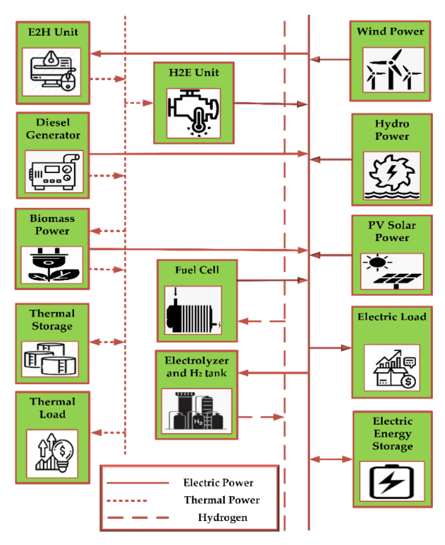
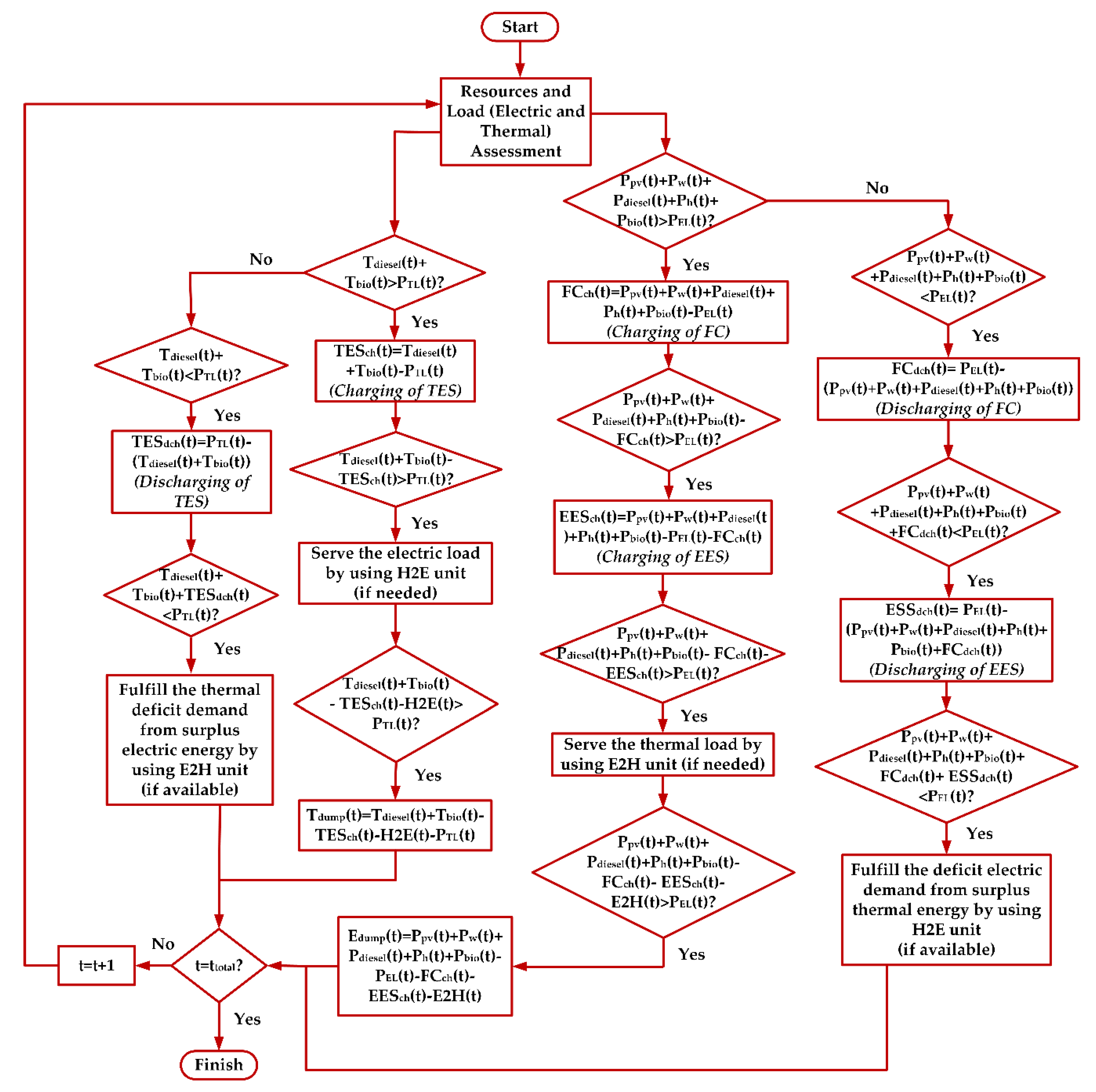
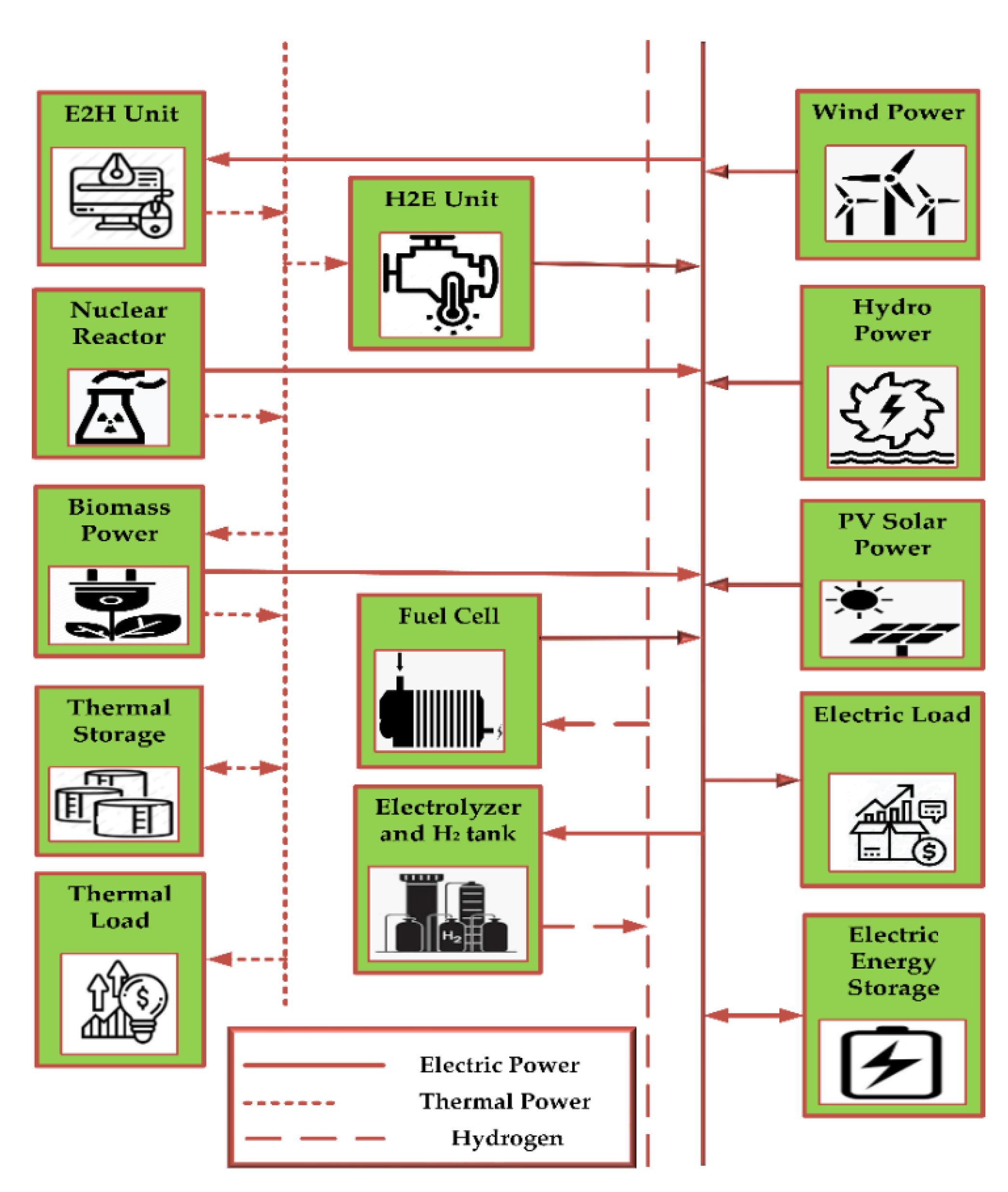
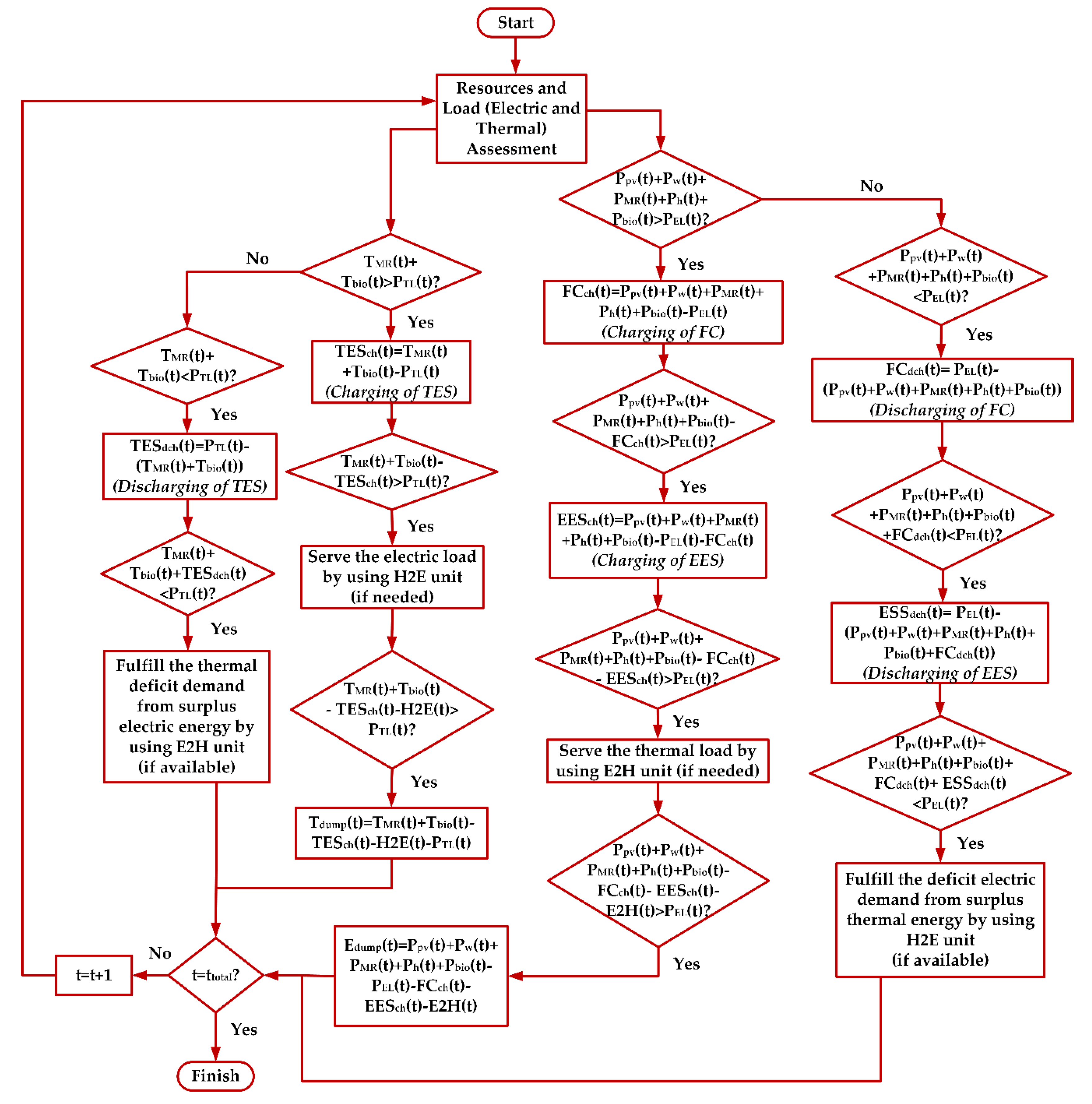
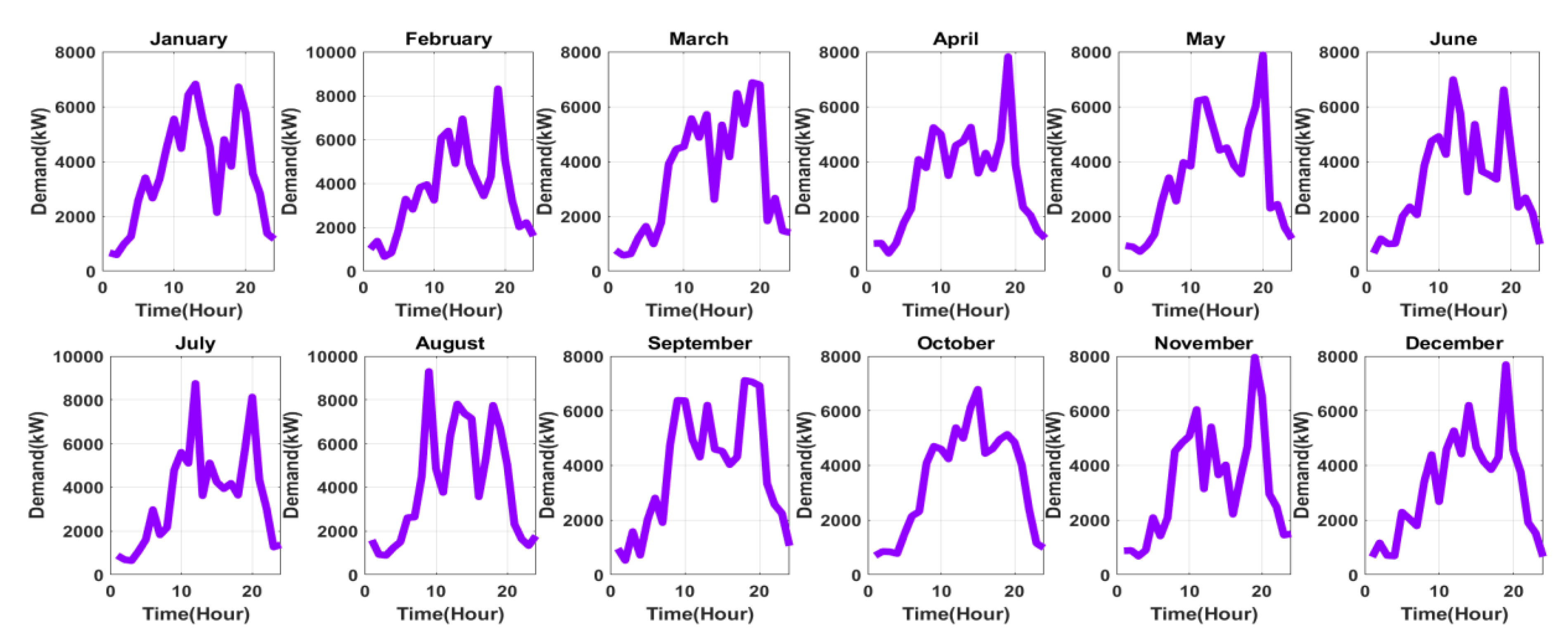
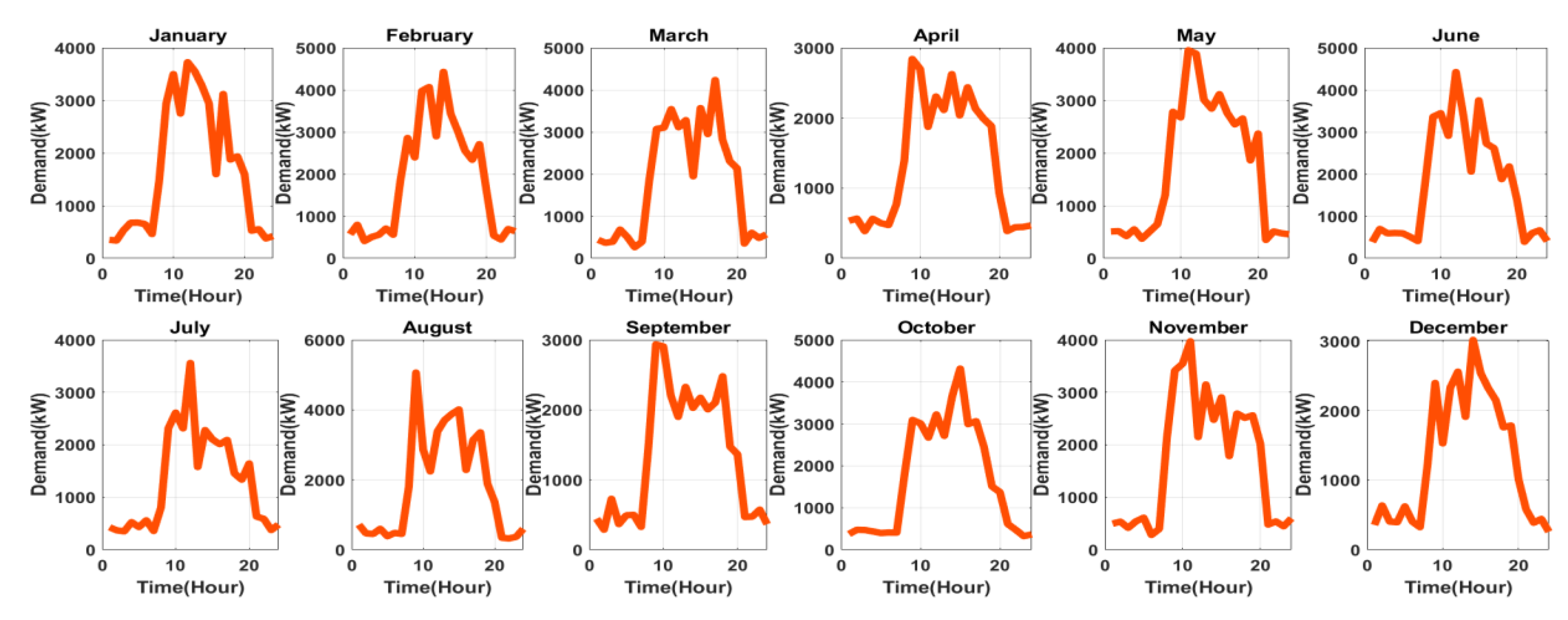
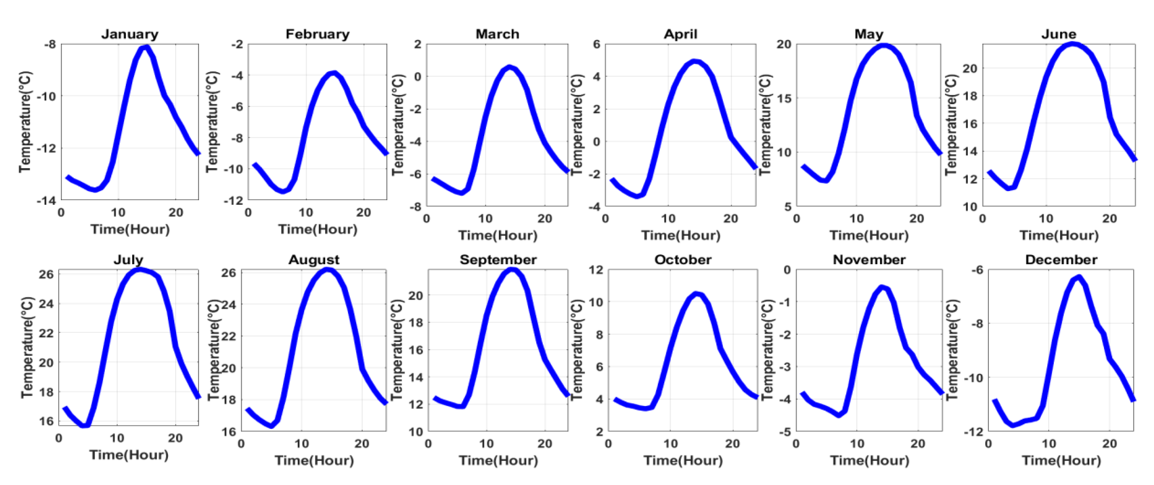
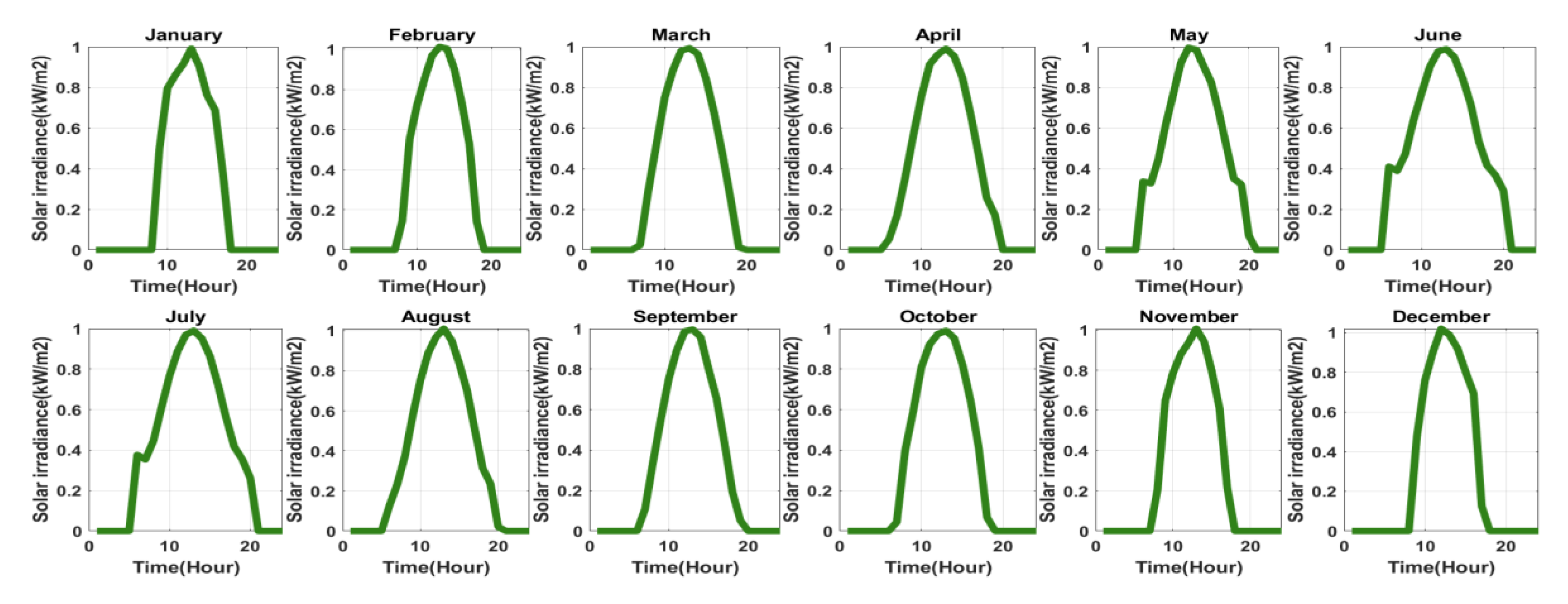
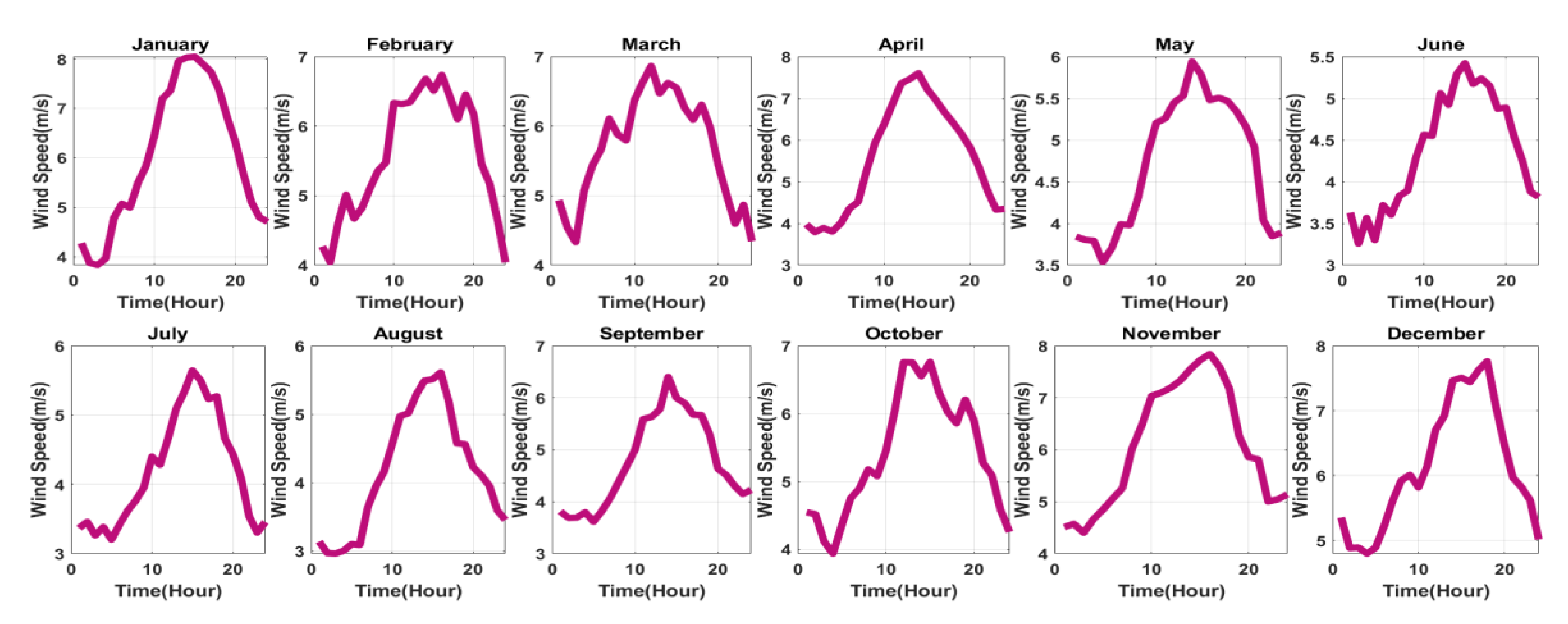
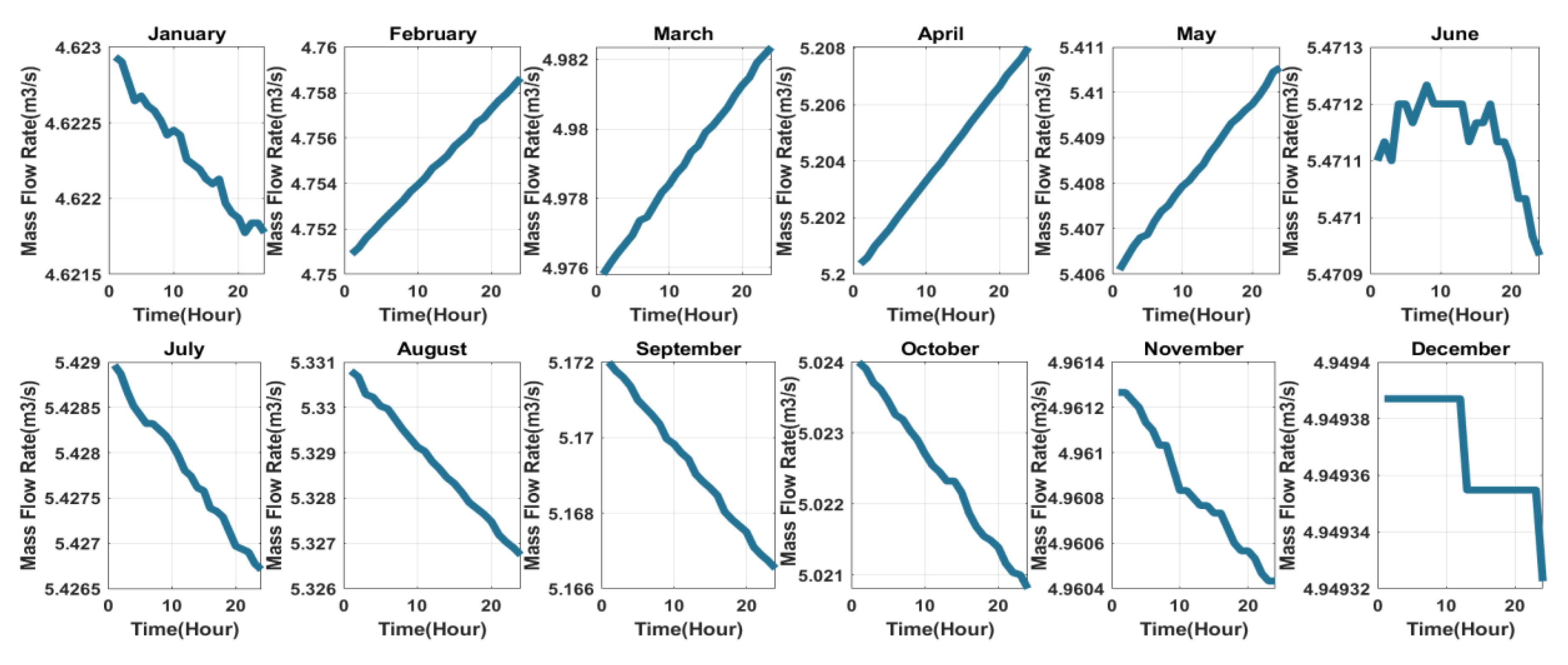
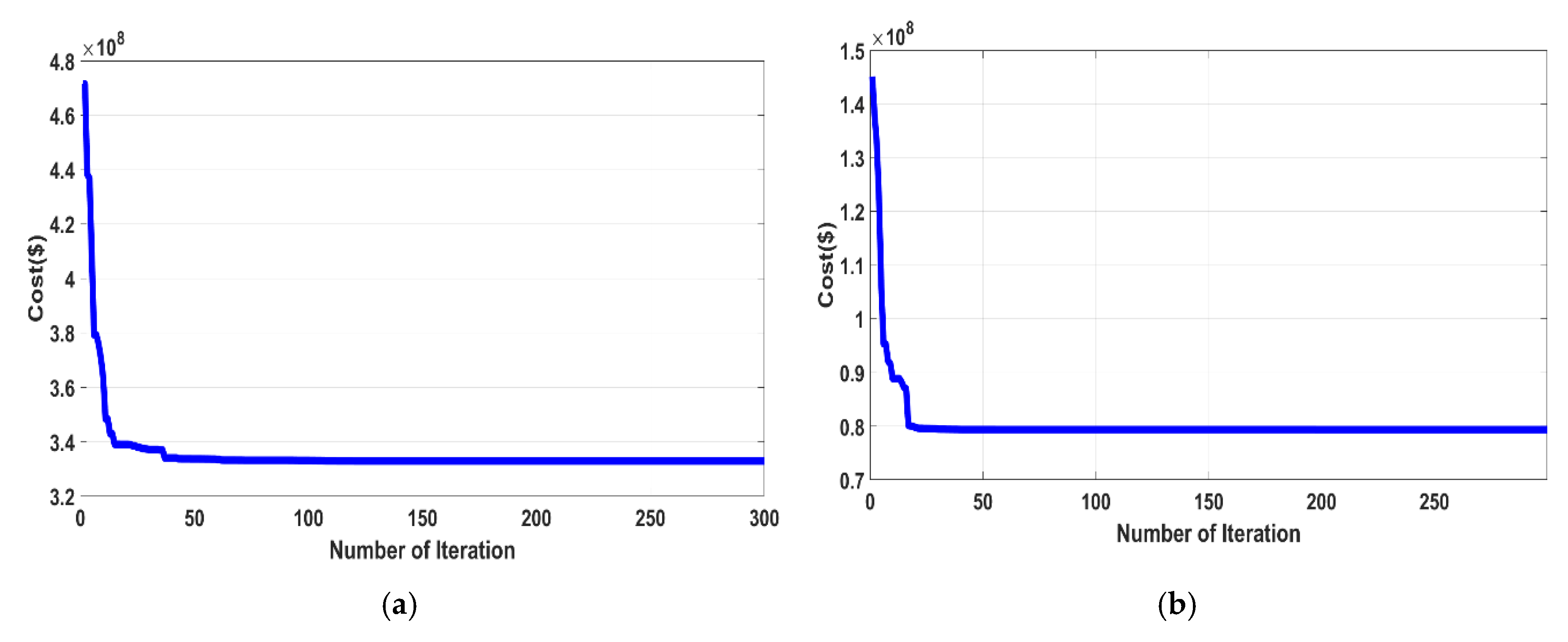
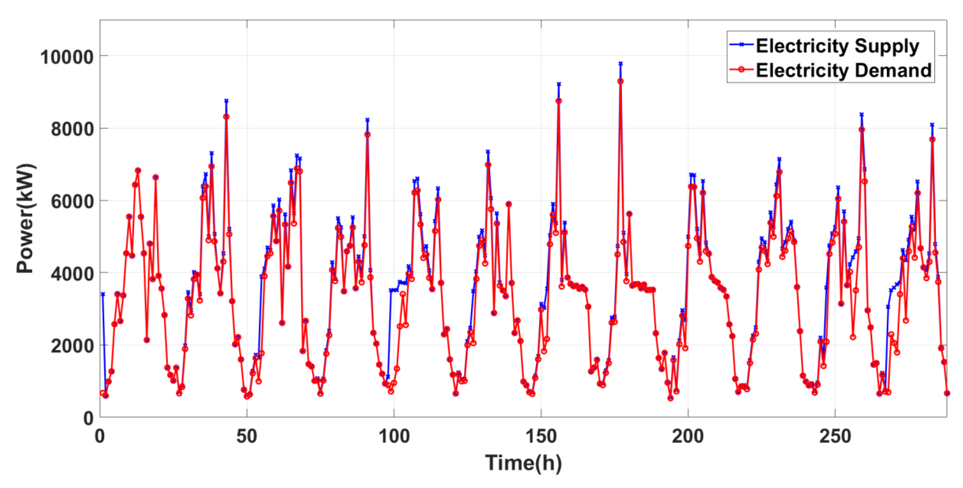
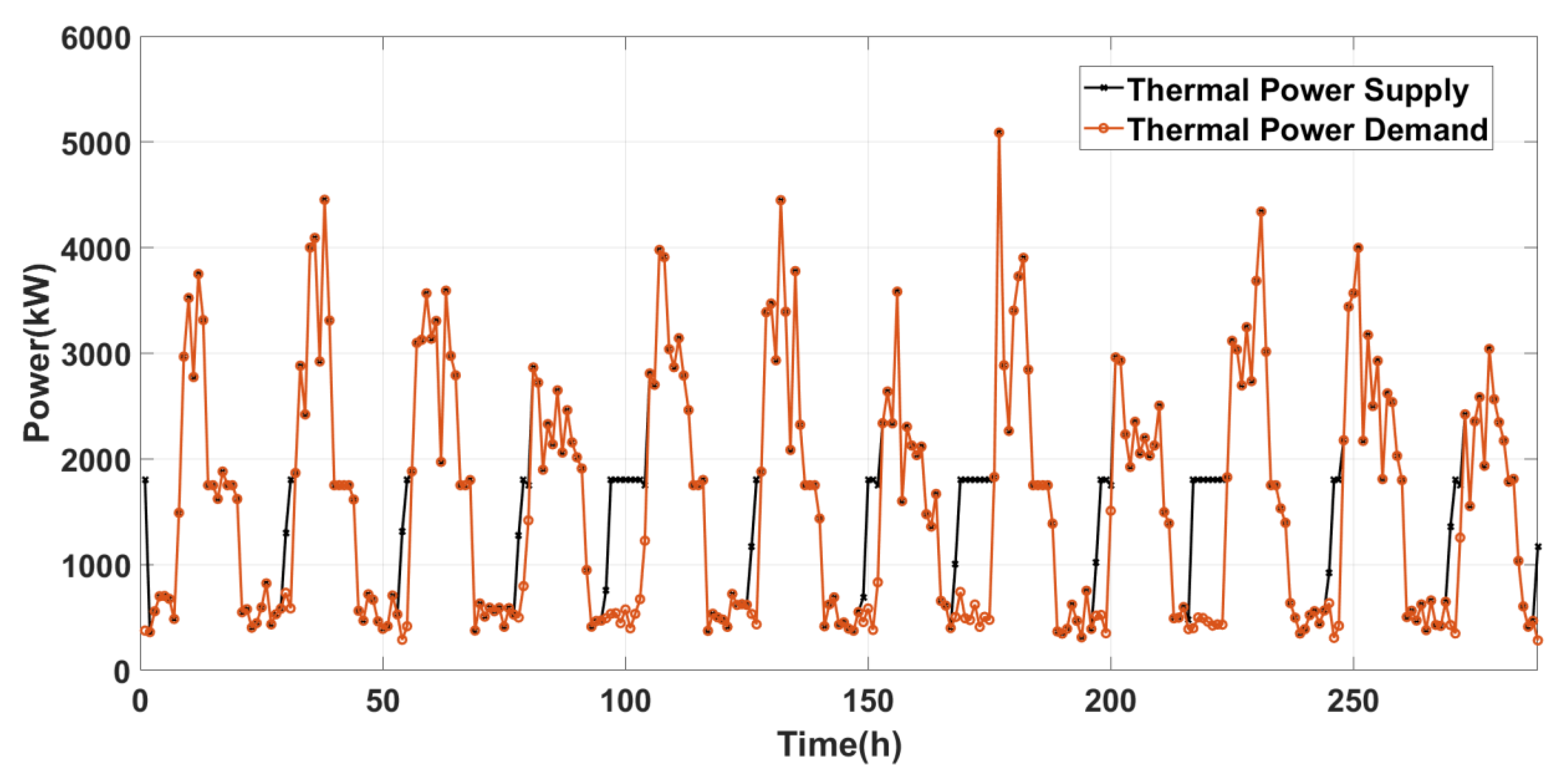
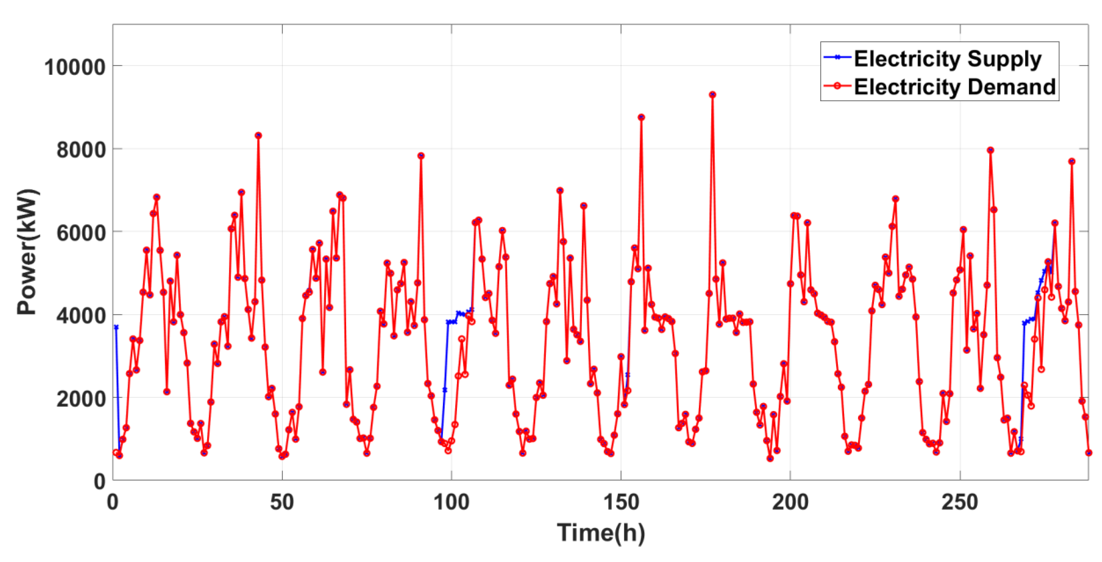
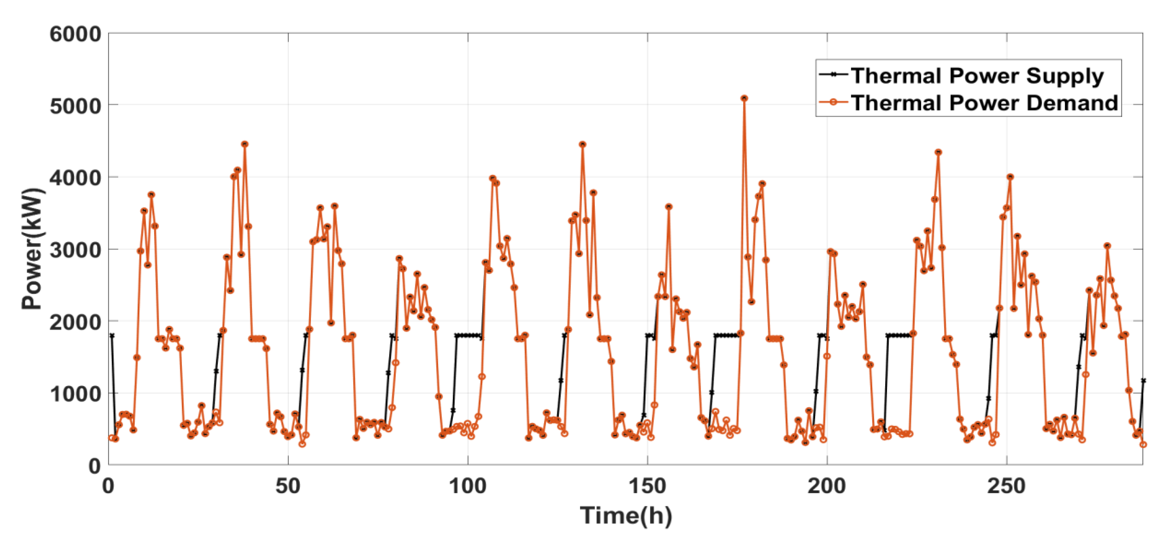
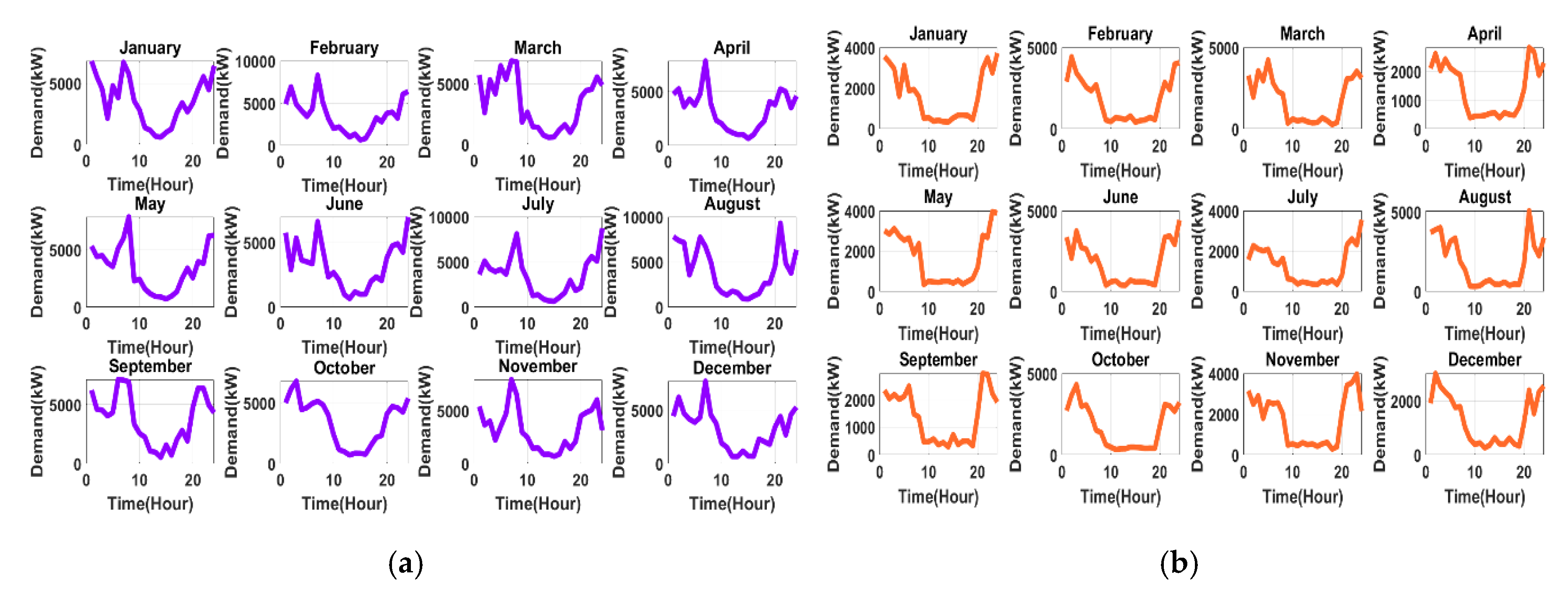
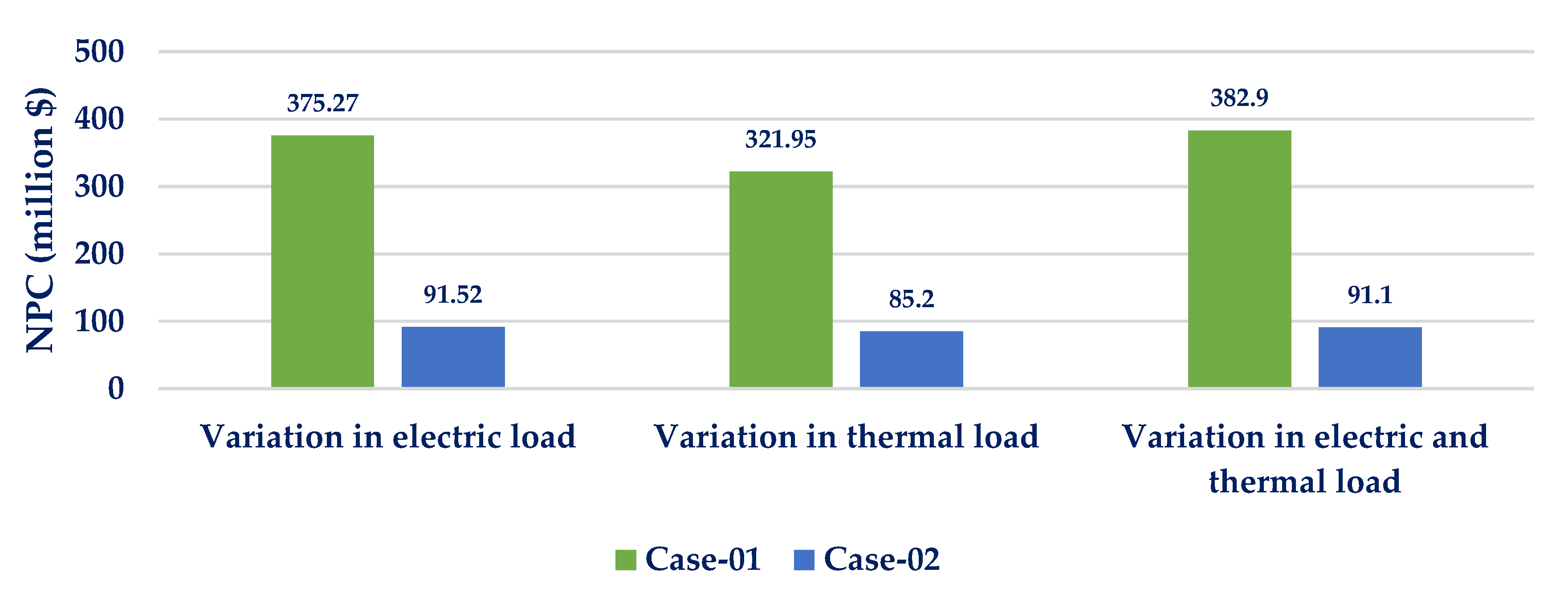
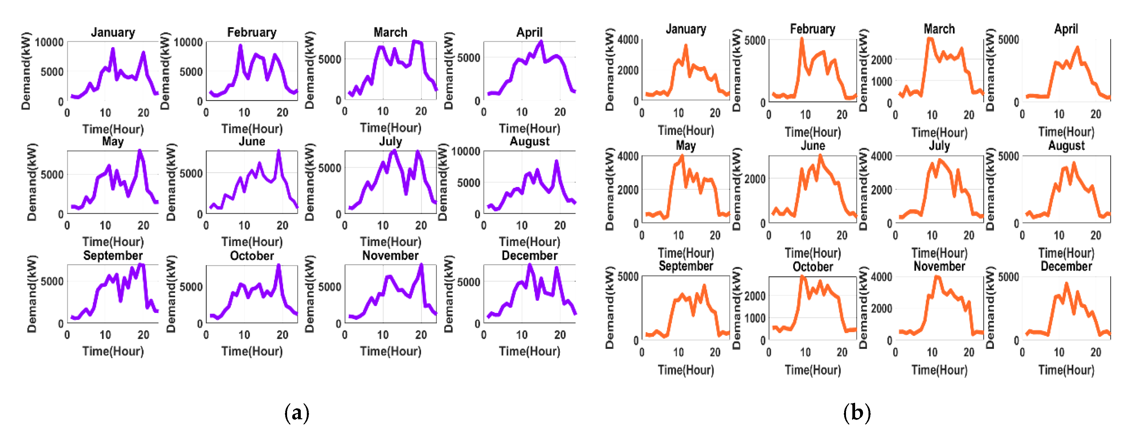
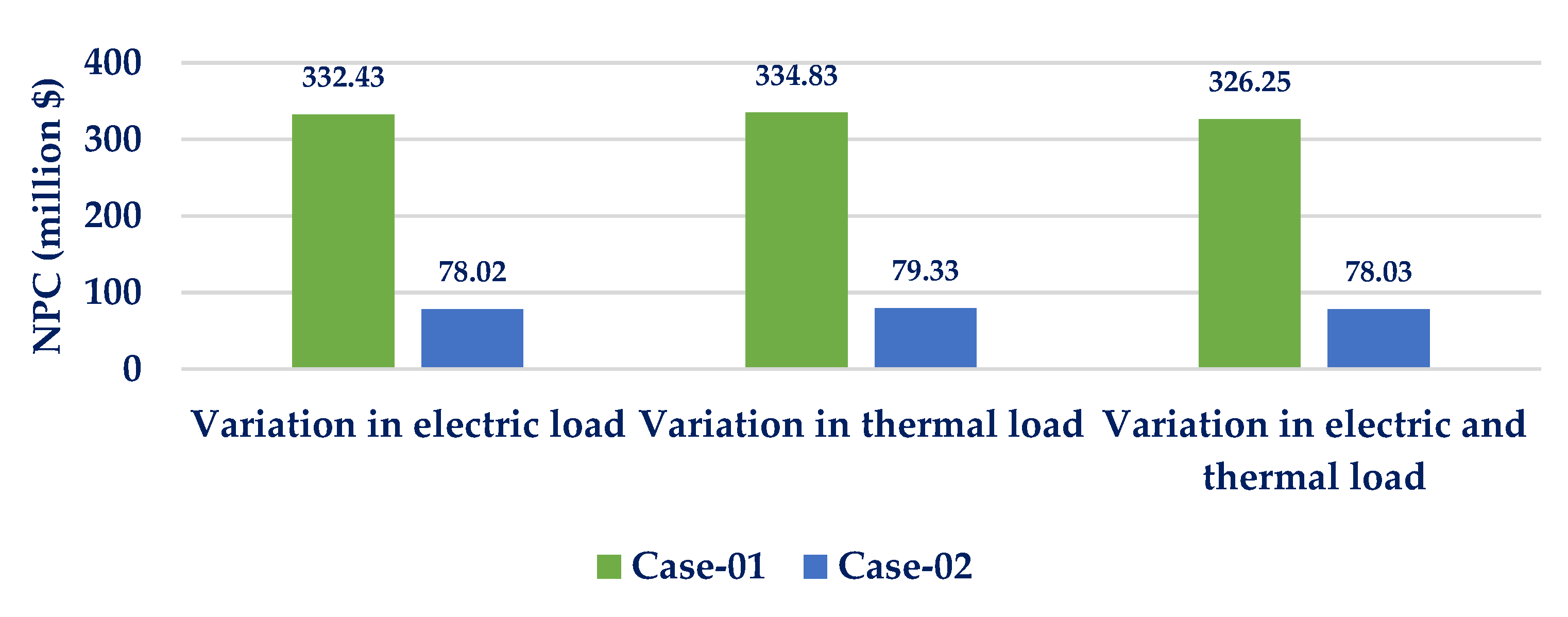
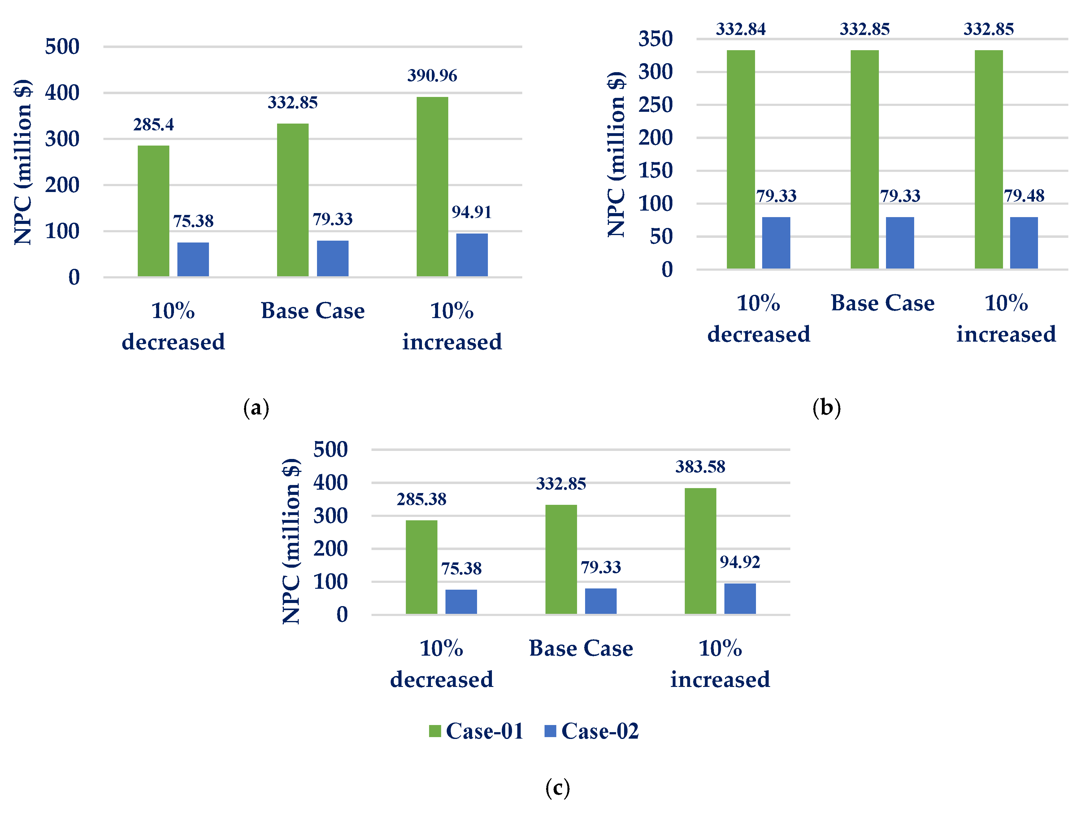
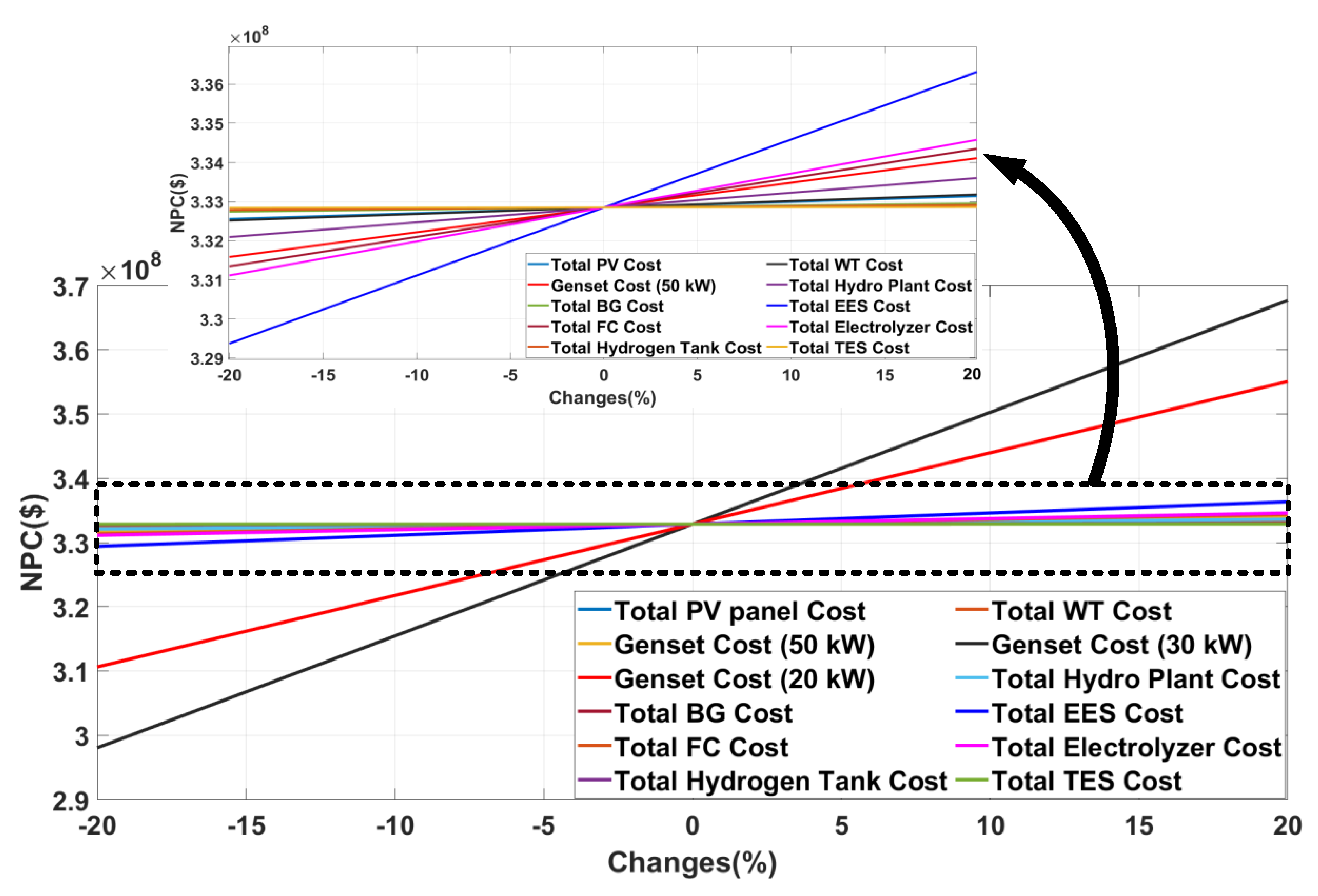
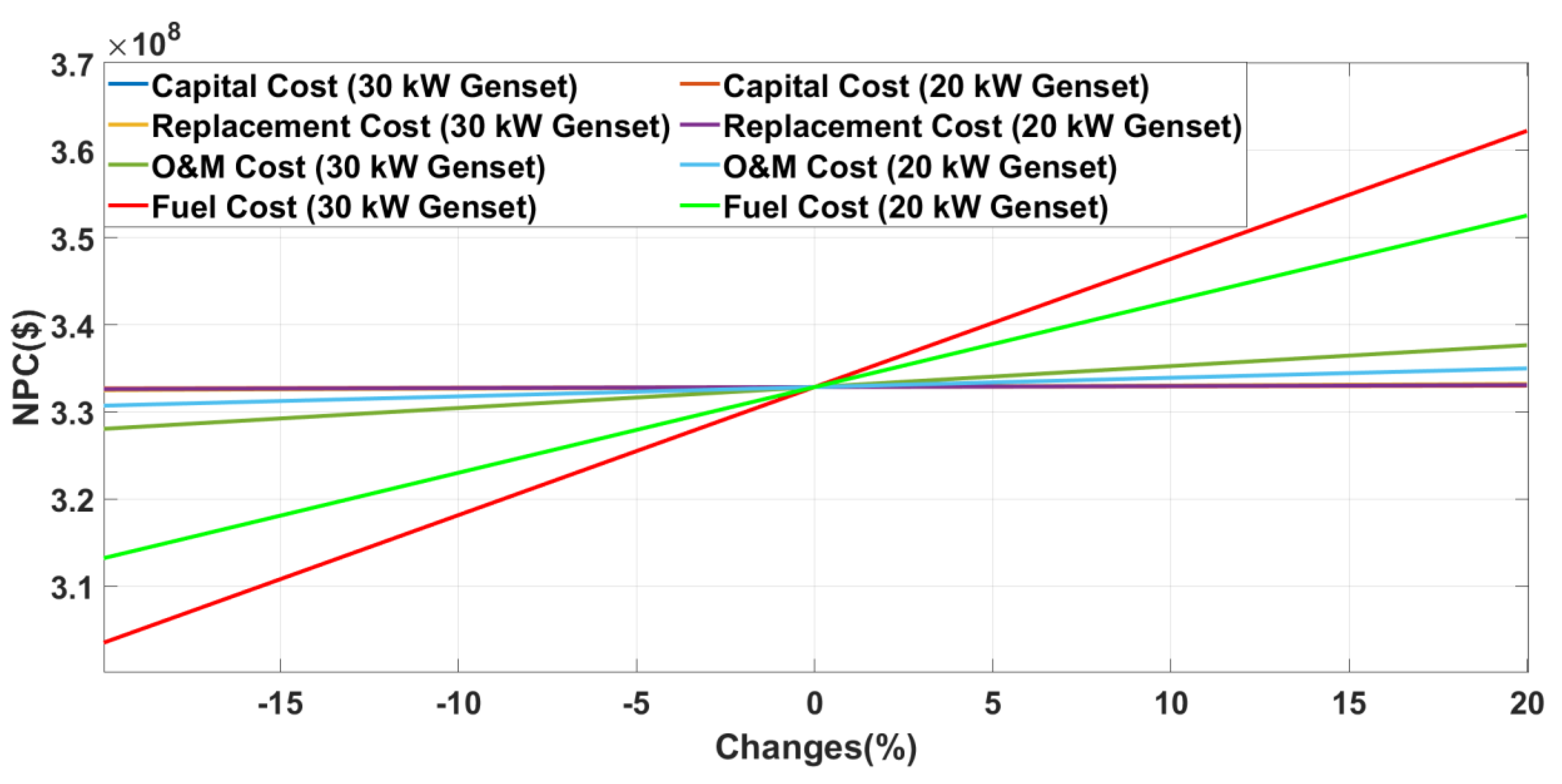
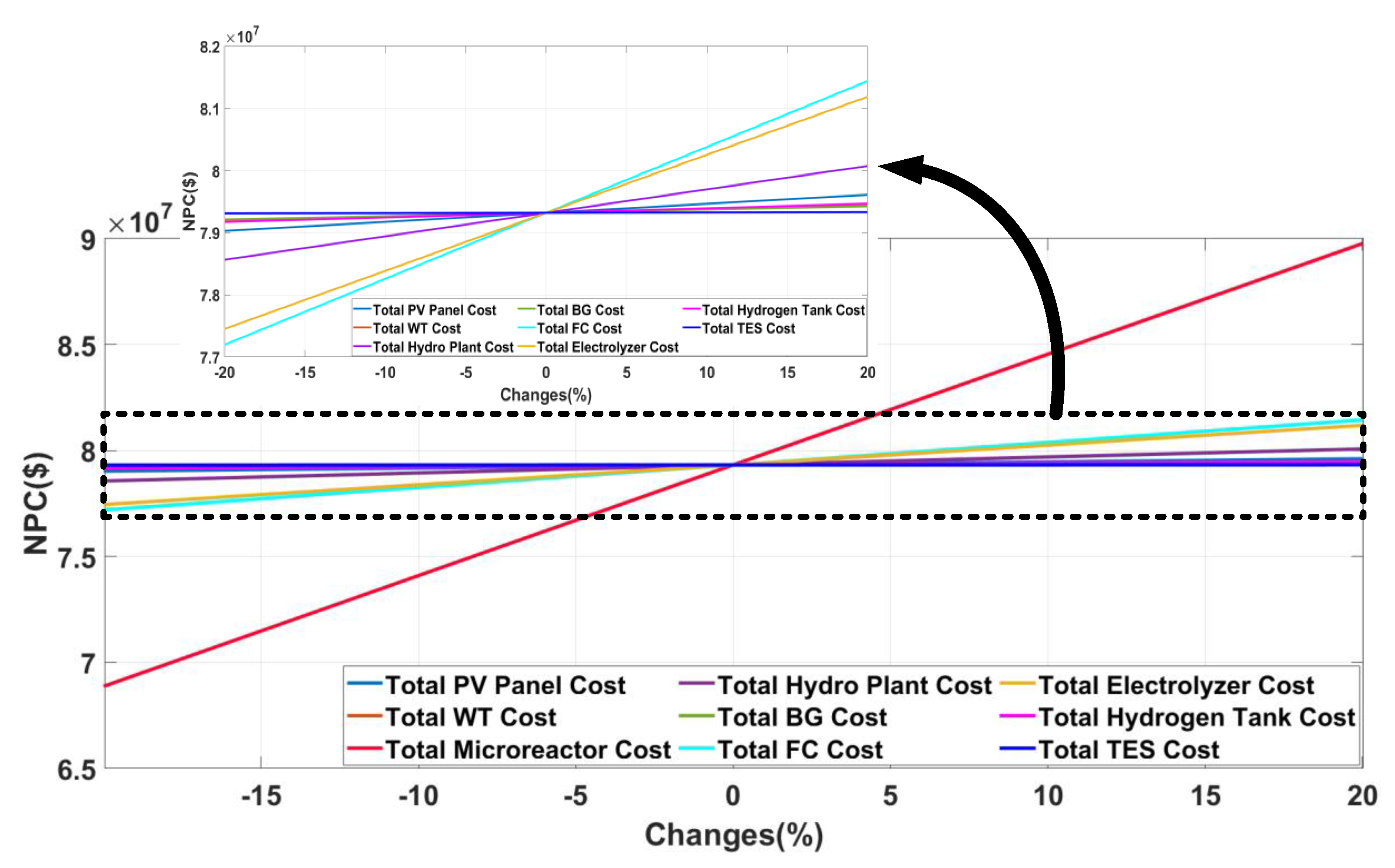
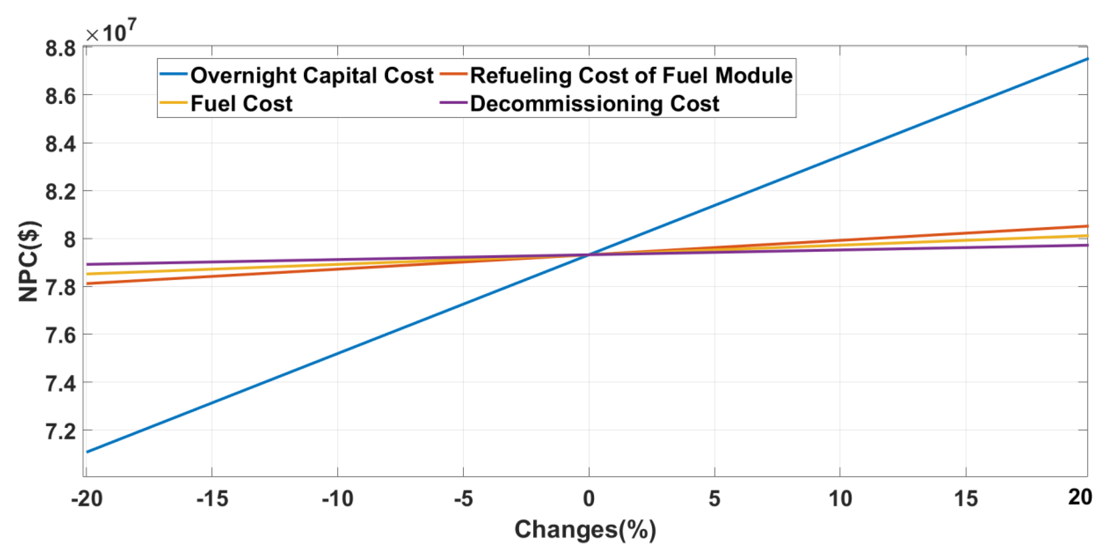
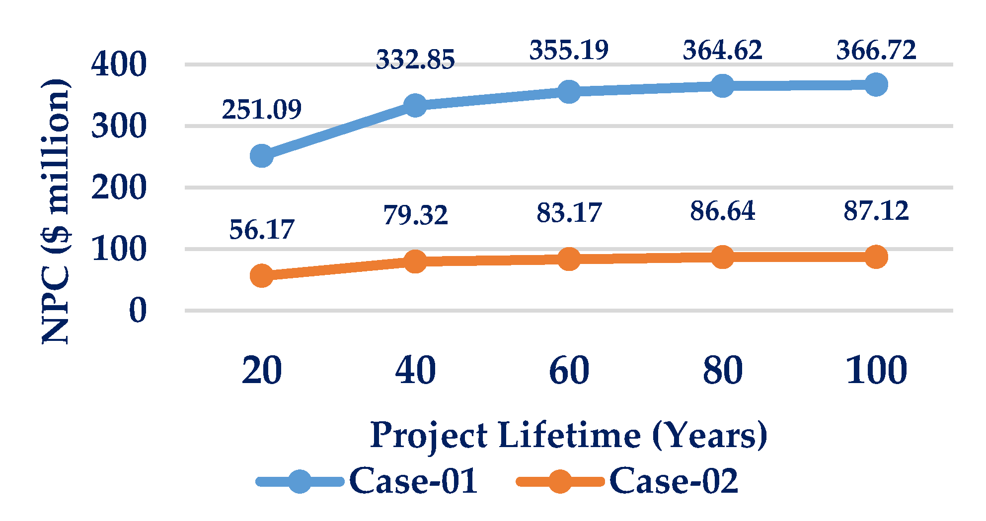
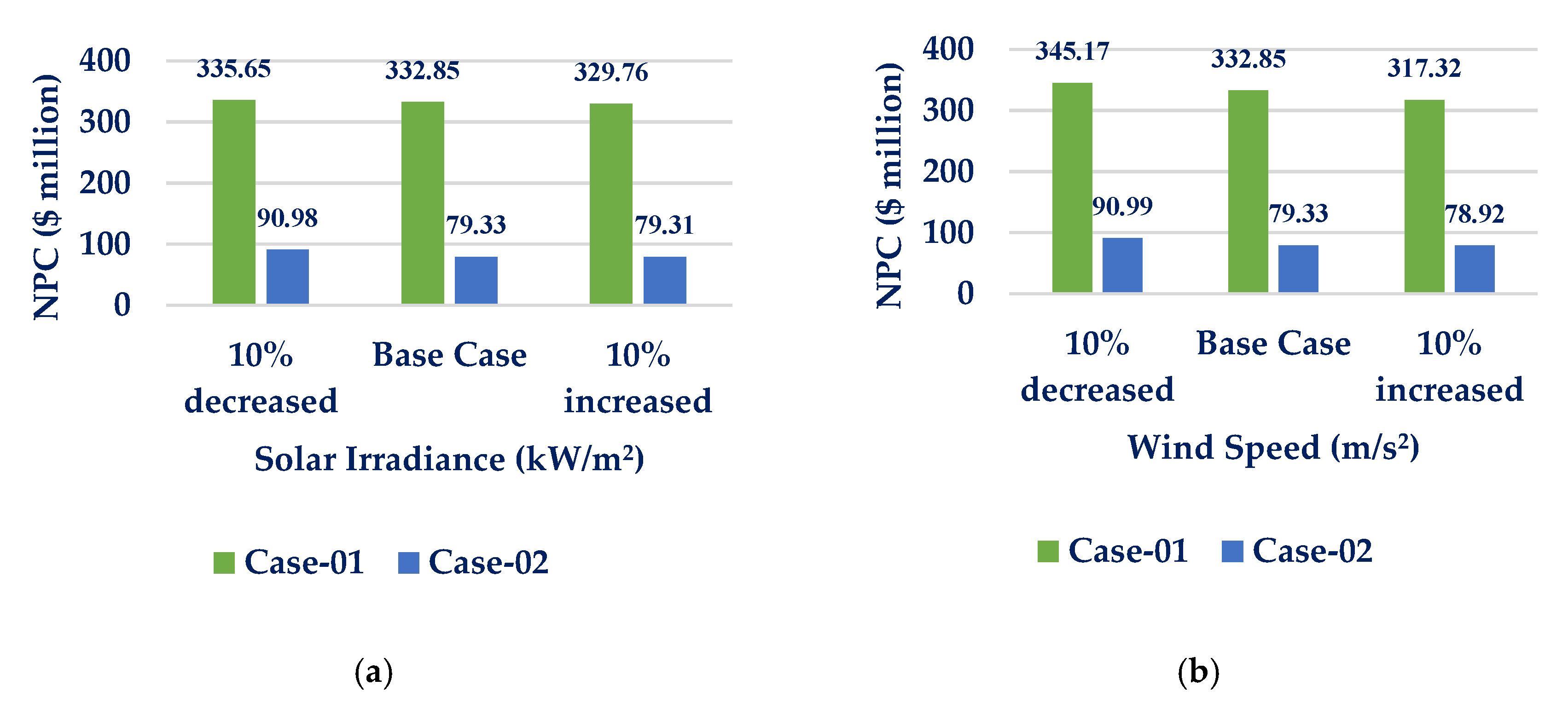
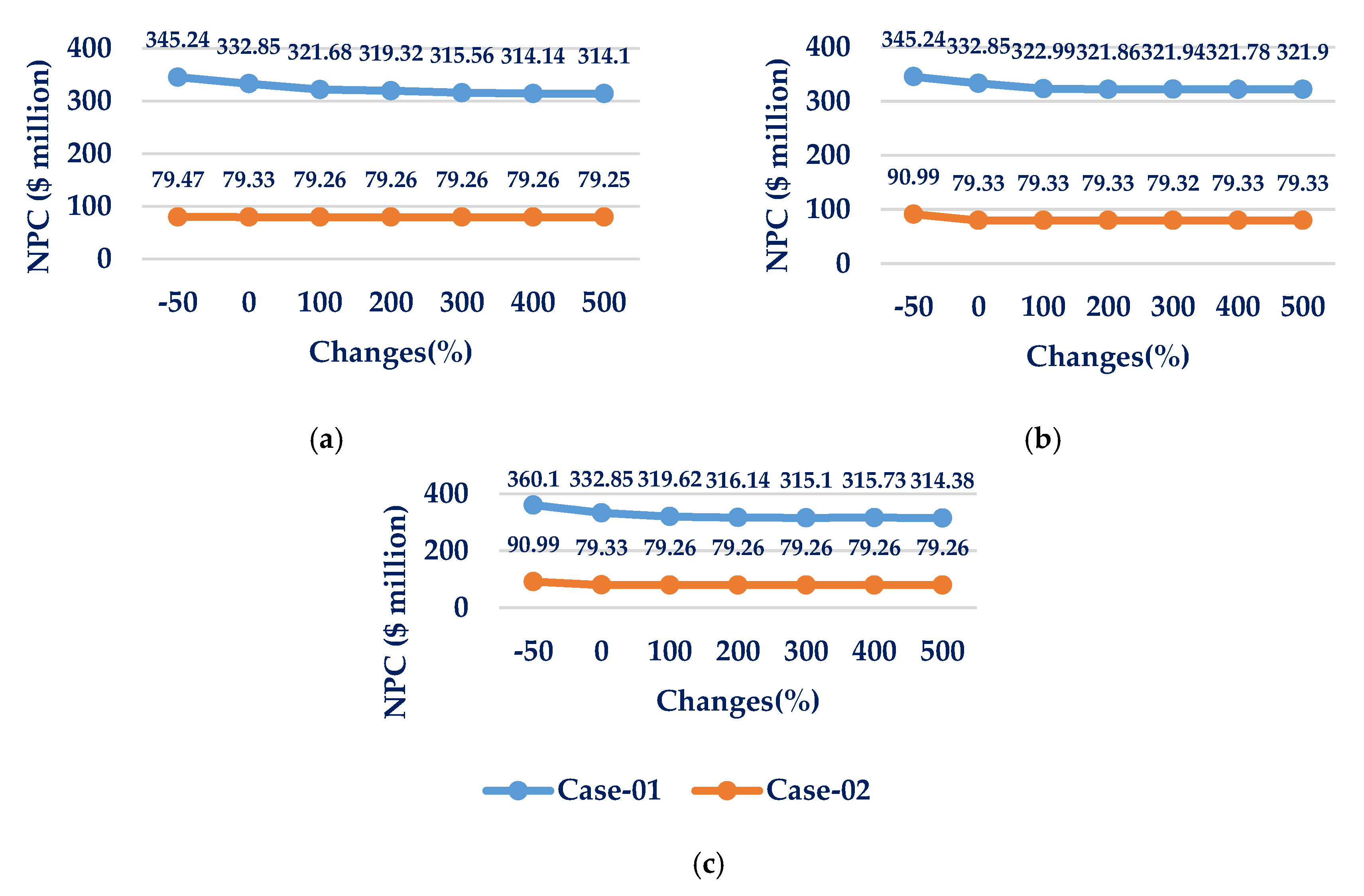
Table 1.
A list of microreactors [34].
Table 1.
A list of microreactors [34].
| Name | Capacity (MWe) | Developer |
|---|---|---|
| eVinci | 0.2–5 | Westinghouse, USA |
| NuScale micro | 1–10 | NuScale, USA |
| Aurora | 1.5 | Oklo, USA |
| Sealer | 3–10 | LeadCold, Sweden |
| Holos Quad | 3–13 | HolosGen, USA |
| U-battery | 4 | Urenco-led consortium, UK |
| MMR-5 | 5 | UltraSafe Nuclear, USA |
Table 2.
Specifications of the MR.
| Parameters | Value | Parameters | Value |
|---|---|---|---|
| ) | 1000 | 20 million | |
| Plant lifetime (Years) | 40 | Core lifetime (Years) | 10 |
| ) | 15,000 | 5 | |
| ) | 350 | Capacity factor (%) | 95 |
| ) | 10 | Plant efficiency (%) | 40 |
Table 3.
Optimal system configuration of Case-01 and Case-02.
| Cases | Case-01 | Case-02 | |
|---|---|---|---|
| Number of particles | 250 | 250 | |
| Number of iterations | 300 | 300 | |
| NPC ($ million) | 332.85 | 79.33 | |
| Number of Diesel Genset/MR | Genset (50 kW) | 1 | 3 (MR) |
| Genset (30 kW) | 50 | ||
| Genset (20 kW) | 50 | ||
| Number of PV panels | 100 | 100 | |
| Number of WT | 100 | 34 | |
| Hydro turbine capacity (kW) | 1000.64 | 1000.64 | |
| Required CHP Efficiency (%) | Genset (50 kW) | 19.8 | 24.6 |
| Genset (30 kW) | 25.8 | ||
| Genset (20 kW) | 30 | ||
| Number of Hydrogen tank | 10 | 23 | |
| Battery bank capacity (MWh) | 15.30 | 0 | |
| TES capacity (MWh) | 19.90 | 19.90 | |
| E2H unit capacity (kW) | 0 | 0 | |
| H2E unit capacity (kW) | 0 | 0 | |
Table 4.
Comparison of KPIs.
| Parameters | Case-01 | Case-02 |
|---|---|---|
| (%) | 5 | 4.36 |
| (%) | 5 | 5 |
| (%) | 10 | 1.83 |
| (%) | 10 | 10 |
| (%) | 111.72 | 116.48 |
| (%) | 108.71 | 108.71 |
| (%) | 91.32 | 90.97 |
| (%) | 81.25 | 79.51 |
| ($/kWh) | 0.4879 | 0.1163 |
Table 5.
A summary of the sensitivity analysis.
| Section | Summary |
|---|---|
| Section 6.1 | This segment compares the NPC of both cases due to the shift in daily peak demand. |
| Section 6.2 | The section assesses the NPC’s sensitivity to the difference in seasonal peak demand. |
| Section 6.3 | This piece of assessment estimates the impact of average demand changes on NPC. |
| Section 6.4 | The section evaluates and identifies the impact of different equipment cost on NPC. |
| Section 6.5 | This sub-section determines the impact of project lifetime on NPC for both cases. |
| Section 6.6 | This segment evaluates the influence of RESs on system planning and NPC. |
| Section 6.7 | The section analyzes the impact on NPC due to variation in PV panel and WT availability. |
© 2020 by the authors. Licensee MDPI, Basel, Switzerland. This article is an open access article distributed under the terms and conditions of the Creative Commons Attribution (CC BY) license (http://creativecommons.org/licenses/by/4.0/).
Share and Cite
MDPI and ACS Style
Gabbar, H.A.; Abdussami, M.R.; Adham, M.I. Micro Nuclear Reactors: Potential Replacements for Diesel Gensets within Micro Energy Grids. Energies 2020, 13, 5172. https://0-doi-org.brum.beds.ac.uk/10.3390/en13195172
AMA Style
Gabbar HA, Abdussami MR, Adham MI. Micro Nuclear Reactors: Potential Replacements for Diesel Gensets within Micro Energy Grids. Energies. 2020; 13(19):5172. https://0-doi-org.brum.beds.ac.uk/10.3390/en13195172
Chicago/Turabian StyleGabbar, Hossam A., Muhammad R. Abdussami, and Md. Ibrahim Adham. 2020. "Micro Nuclear Reactors: Potential Replacements for Diesel Gensets within Micro Energy Grids" Energies 13, no. 19: 5172. https://0-doi-org.brum.beds.ac.uk/10.3390/en13195172
Note that from the first issue of 2016, this journal uses article numbers instead of page numbers. See further details here.