Aerodynamic Study of the Wake Effects on a Formula 1 Car


LABSON—Department of Fluid Mechanics, Universitat Politècnica de Catalunya, ES-08222 Terrassa, Catalunya, Spain
*
Author to whom correspondence should be addressed.
Energies 2020, 13(19), 5183; https://0-doi-org.brum.beds.ac.uk/10.3390/en13195183
Submission received: 7 September 2020
/
Revised: 21 September 2020
/
Accepted: 23 September 2020
/
Published: 5 October 2020
(This article belongs to the Special Issue The Numerical Simulation of Fluid Flow)
Abstract
:The high complexity of current Formula One aerodynamics has raised the question of whether an urgent modification in the existing aerodynamic package is required. The present study is based on the evaluation and quantification of the aerodynamic performance on a 2017 spec. adapted Formula 1 car (the latest major aerodynamic update) by means of Computational Fluid Dynamics (CFD) analysis in order to argue whether the 2022 changes in the regulations are justified in terms of aerodynamic necessities. Both free stream and flow disturbance (wake effects) conditions are evaluated in order to study and quantify the effects that the wake may cause on the latter case. The problem is solved by performing different CFD simulations using the OpenFoam solver. The significance and originality of the research may dictate the guidelines towards an overall improvement of the category and it may set a precedent on how to model racing car aerodynamics. The studied behaviour suggests that modern F1 cars are designed and well optimised to run under free stream flows, but they experience drastic aerodynamic losses (ranging from −23% to 62% in downforce coefficients) when running under wake flows. Although the overall aerodynamic loads are reduced, there is a fuel efficiency improvement as the power that is required to overcome the drag is smaller. The modern performance of Ground Effect by means of vortices management represent a very unique and complex way of modelling modern aerodynamics, but at the same time notably compromises the performance of the cars when an overtaking maneuver is intended.
1. Introduction
For many years, it has been openly stated that F1 has lost much of its spectacular nature due to the difficulty of the cars in being able to follow each other closely for a long period of time. The sophisticated aerodynamics of these single-seater cars has compromised the chasing of the leading car (mostly due to the turbulent wake generation and clearly disturbed flow [1]). This way, it was found to be convenient to numerically analyse and quantify the actual loss of aerodynamic loads on a F1 car due to the immediate presence of a rival in front of it and then, establish a fair comparison with the situation of a free stream condition.
In recent years, a significant number of investigations has been performed, both conducted by the Federation Internationale de l’Automobile (FIA) or Formula One teams and by other sources of investigation. The works of Ravelli and Savini [2,3] have been taken as a reference, as they are considered to be a feasible approach to such a complex CFD problem as the very same CAD (Computer Aided Design) model is evaluated. The obtained results show interesting vorticity behaviours and the reference data for the comparison of their numerical results under free stream flows are taken into account in this manuscript.
Besides, the works of Newbown, et al. [4] and Perry, et al. [5] have set a positive precedent on how to numerically evaluate a F1 car under wake flows, despite using a quite outdated CAD geometry. The methodology that they applied, consisting of varying the different distances between cars, is taken as a good inspiration on how to operate with the present model. However, it is believed that studying closer distances between the cars under the wake flows could potentially give a more complete definition of the study. That is why the closest distance that is evaluated between the two cars on the present manuscript is around a quarter of a car length, which is significantly smaller that the ones that are reflected on other publications.
Other authors, such as Ogawa et al. [6] or Senger et al. [7], have also contributed to the definition of the whole methodology applied this CFD study. Special attention is also placed on the research carried out by Larsson [8] that was backed by the BMW Sauber F1 team, where the description given of the wing interaction with the tire wake is crucial for the understanding of the on-set flow to the underbody.
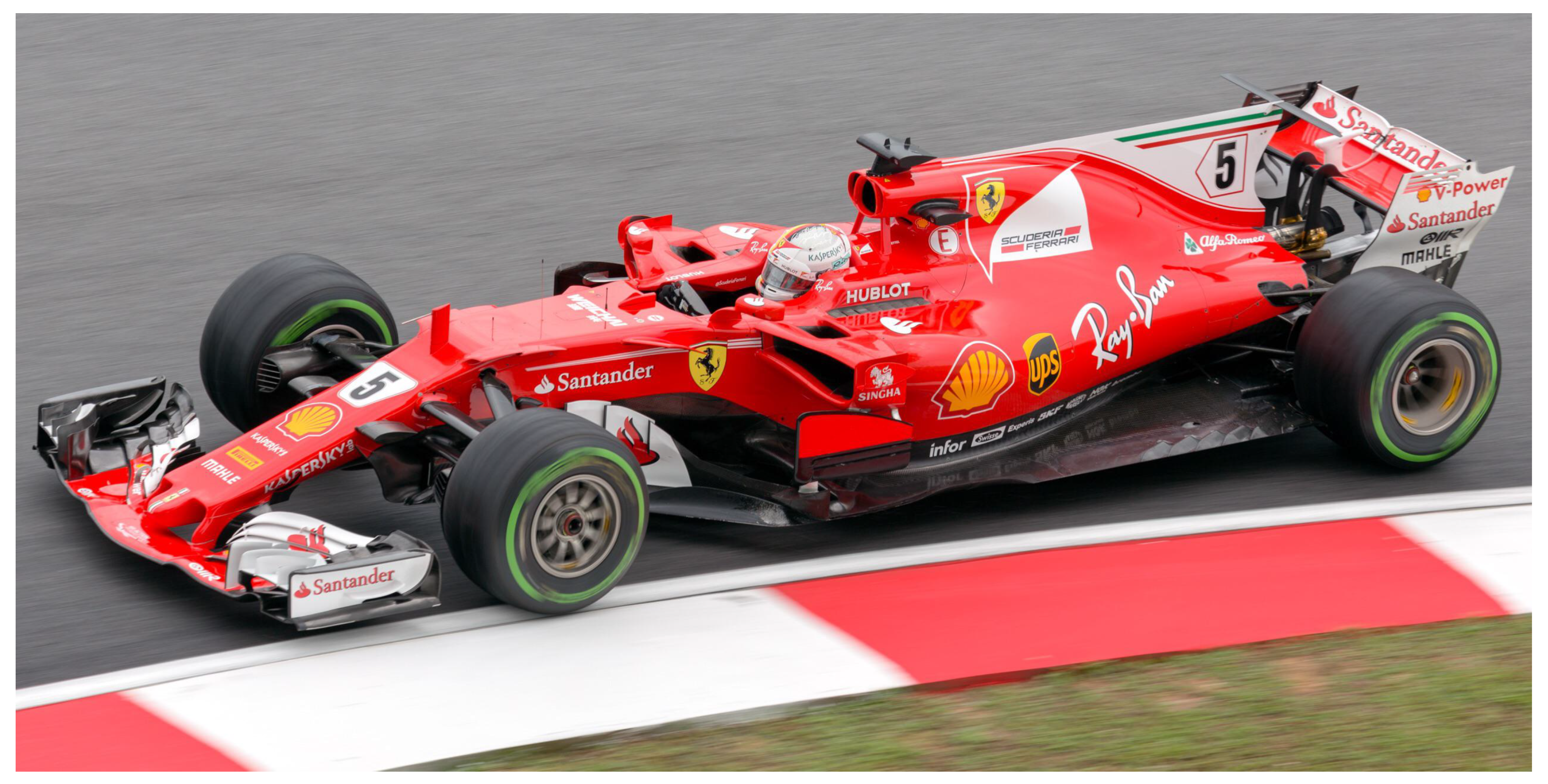
The main contribution and goal of this paper is to evaluate, study, and numerically quantify the aerodynamic performance of a 2017 spec. adapted F1 car (see Figure 1) under free stream conditions and wake flows with the purpose of being able to argue whether the 2022 changes in the regulations are somehow justified in terms of aerodynamic necessities. In addition to, an original approach is given when including some energetic calculations, so as to see how the fact of running under wake flows can harm or benefit the overall power requirements and, therefore, affect the fuel efficiency of the cars.
This work can be considered to be contemporary study, as very few sources have extracted meaningful conclusions regarding the latest F1 aerodynamic package. Accordingly, the originality of this work recalls on the judgement that the authors may offer on the present F1 regulations, so as to contribute to a significant upcoming improvement of the category.
The CFD methodology is primarily selected as other resources, such as the use of a wind tunnel or any other experimental solutions, are currently out of reach to deal with such a study (see Newbon et al. works in [10]). The amount of energy resources that a wind tunnel experimental execution would require (without mentioning the environmental impact of its construction) is also a fundamental point to opt for a more sensible approach. Moreover, as the CFD discipline involves a rather strict and accurate process to be able to deal with external aerodynamic problems, the methodology is accepted in order to discern and evaluate the hypothesis established. It has to be commented, though, that CFD models are usually calibrated (see [11,12]), but for the present research, it was not possible. Accordingly, a future investigation regarding the usage of experimental data acquisition would validate this approach.
2. Materials and Methods
Computational Fluid Dynamics is the branch of Fluid Mechanics that uses numerical methods and algorithms so as to solve and analyse the behaviour of the fluids. In order to benefit from CFD techniques, it is quite important to know as much as possible regarding the real problem that is intended to be simulated (this are the physical properties of the fluid, the boundary conditions as well as other variables). Moreover, CFD involves the design of a CAD model to be meshed and eventually solve a compendium of mathematical equations on it, as they are the fundamental tool to solve in numerical problems. However, some drawbacks that are inherent to CFD involve the model calibration (to ensure reliable results), complex meshing and usually powerful CPU requirements, among others.
Two different scenarios were initially contemplated within the evaluation of the present work. A free stream approach, where the behaviour of the F1 car is analysed under optimal conditions and a more challenging one, based on a conditioned situation under wake flows. As for the latter, different distances were evaluated in order to appreciate the changes and behaviour of the car in second place in direct comparison with the leading car.
2.1. Geometry
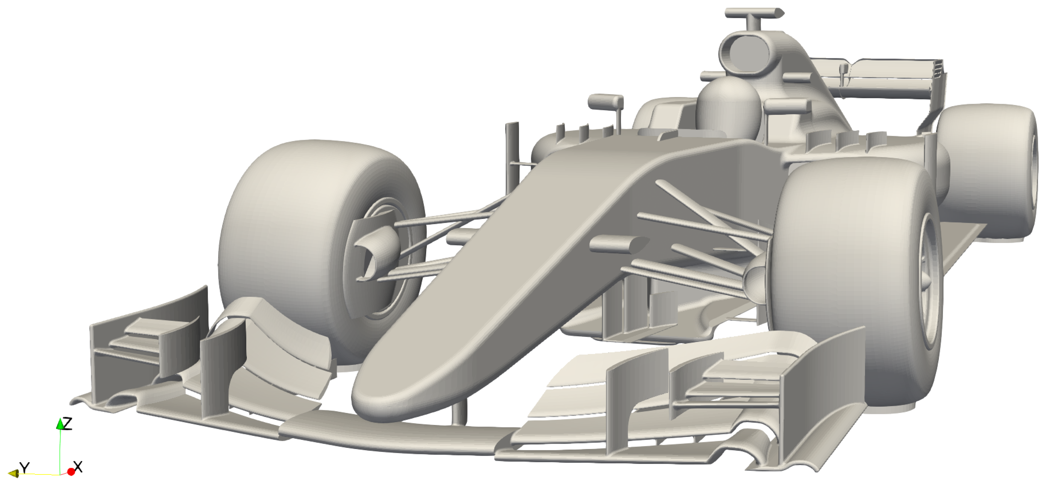
The CAD geometry employed was the PERRIN F1 car [13], as it was a realistic approach to a real F1 car because it was designed under the 2017 FIA regulations. This includes several small realistic details, such as winglets, vanes, vorticity generators and slots, being the smallest elements 1.5 mm thick. The length L of the car, which is later considered for the dimensions of the overall domain is around 5.350 m, while its wheelbase, required for the turbulent length scale measures 3.745 m. The geometry was exported to Parasolid format (.x_t.), so as to be processed by the SnappyHexMesh command. Figure 2 displays a generic view of the aforementioned F1 car.
2.2. Solver
The simulations were executed using the OpenFoam [14] toolbox that solves the equations for unsteady incompressible flow of mass and momentum presented in Equation (1), (also known as Navier–Stokes equations [15]); as well as the continuity equation shown in (3).
where
The discretisation of the domain was obtained applying the FVM (Finite Volume Method), as this method is locally conservative due to being based on a balance approach [16]. The gradient, divergence, and laplacian terms of the Navier–Stokes equations were discretised by means of the Gaussian schemes: at cell interfaces, the interpolation schemes were linear (upwind).
On the other hand, the simpleFoam algorithm (Semi-Implicit Method for Pressure-Linked Equations) was the one chosen, as it is appropriate for incompressible, steady, turbulent flows. The reason why a steady solver was applied on a flow field with unsteady characteristics resides in the nature of turbulence, which is, by definition, non-stationary. Accordingly, the presented results (wake vortices among others) are averaged on a medium flow, which is what simpleFoam solves. The goal was not to study transient phenomena (which could be the subject for future works), but these averages to evaluate the effect on average stability of the car.
The GAMG (Geometric Algebraic Multi Grid) solver was utilised for the pressure equation, while smoothSolver was the one that was selected for velocity and turbulence variables.
As for the execution, the initial 800 iterations were performed under a first order discretisation, while the remaining ones were performed using second order schemes.
For the turbulence model, the k- SST (k- is used in the outer region of and outside of the boundary layer and k- is used in the inner boundary layer [17]) was selected, since it offered a faster convergence and better results as compared to k- and Spart Allmaras.
2.3. Domain and Mesh
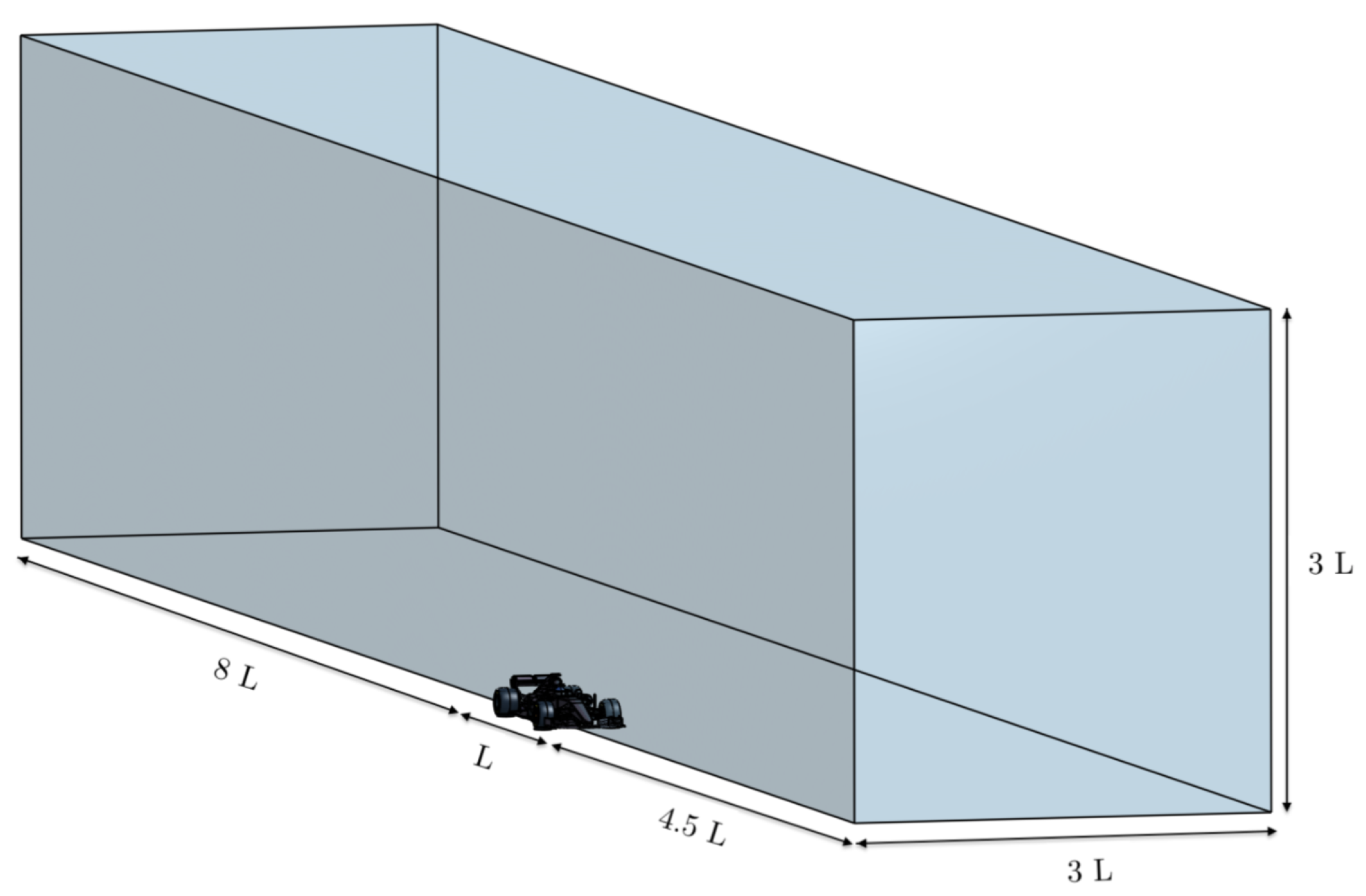
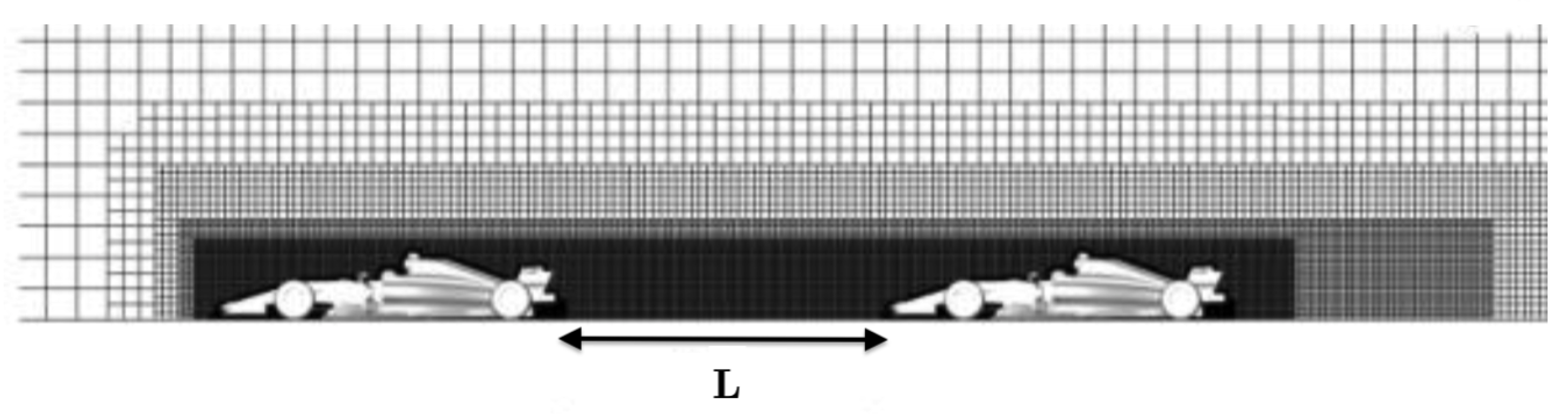
The fluid domain dimensions were inspired by other publications, such as Broniszewski’s [18], who puts special attention to the back region of the domain in order to be able to capture the generation of the wake properly. Figure 3 shows the boundaries of the problem.
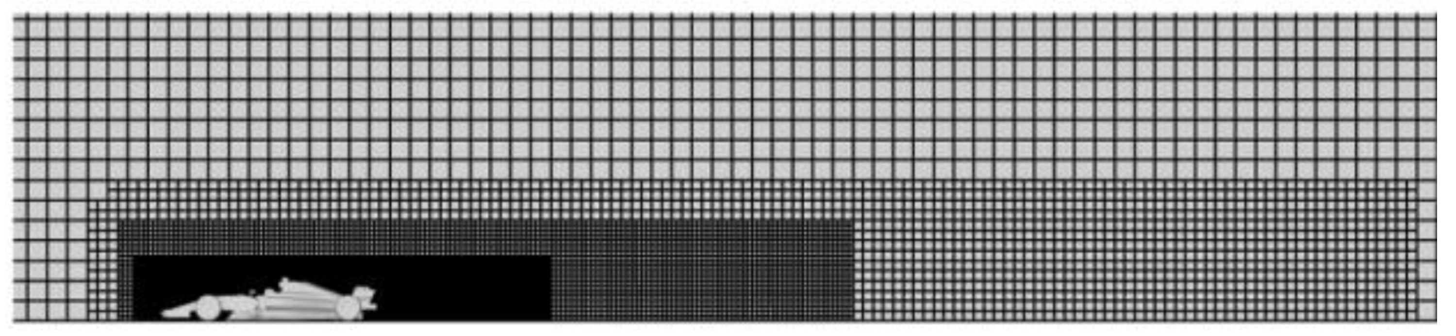
A three dimensional hexahedral mesh by means of the snappyHexMesh and blockMesh commands was generated. The height of the first cell at the solid surfaces is set at 0.01 mm with a layer expansion ratio of 1.3. The resulting average value of y+ is around 40, which involves the use of wall functions as opposed to a near wall treatment, which generally adopts y+ around 1 when solving for low Reynolds (Re) number [19].
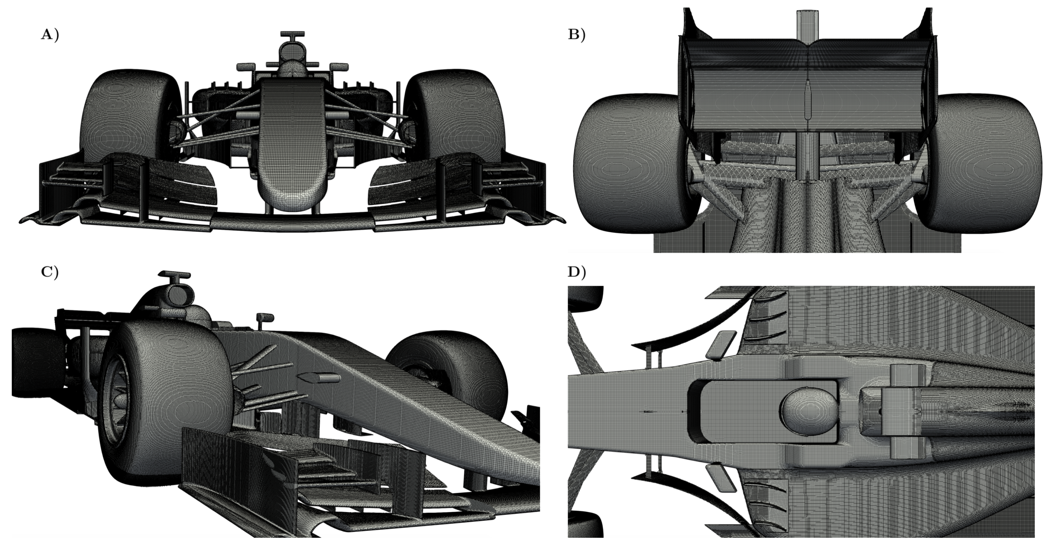
Many refinement enclosures were specified along the geometry in order to be able to capture the effects of the wake and and other phenomena. Special attention was placed in the massive wake region as well as on the downforce generation zones, such as the wings and floor. The results of the mesh procedures may be checked in Figure 4, Figure 5 and Figure 6.
A Grid Convergence Index (GCI) has been calculated in order to guarantee that the analysis of the results that were obtained was independent of the grid size. The GCI methodology is performed according to Celik et al. [20] and the study is performed by varying the level of definition of the three different meshes studied. The refinement levels used range from 5–6 in the coarsest, 6–7 in the intermediate, and 7–8 in the finest. The value analysed corresponds to the lift coefficient multiplied by the surface (). Table 1 presents the results obtained of the GCI.
The GCI values are in the asymptotic range of convergence, both and , as shown in Table 1. It is as well possible to note that the difference in values between the finest and intermediate meshes is considerably small thus, obtaining a rather small percentage of error. As for the computational resources, the finest mesh (which is formed by 19.2 million cells in the free stream case and around 40 million under wake flows) took an approximated time of 8 and 14 hours respectively to be generated. The grid size is found to be reasonable as it is almost identical to the one with which the results are later compared to (see Section 3). Hence, as computational resources do not suppose a huge compromise nor restriction, it was preferred to choose the finest mesh for the following study. The sacrifice in computational time and consumption was notably overcome by the superior amount of detail and definition that the finest mesh could deliver.
2.4. Boundary Conditions
The general boundary conditions established are as follows:
- Inlet velocity set at 50 m/s, as it corresponds to a value which can be easily replicated in a wind tunnel (for experimental validation purposes).
- Pressure outlet set at Atmospheric pressure.
- Symmetry plane.
- Ground velocity set at 50 m/s.
- Slip condition on the side wall and the top of the fluid domain.
- Angular velocity and rotational axis of the wheels (MRF).
2.5. Simulation Performance
The simulations were executed in a cluster that was equipped with 32 cores and 64 Gb of RAM memory and the post-processing operations were carried out by means of an i7 six core laptop with 16 Gb of RAM.
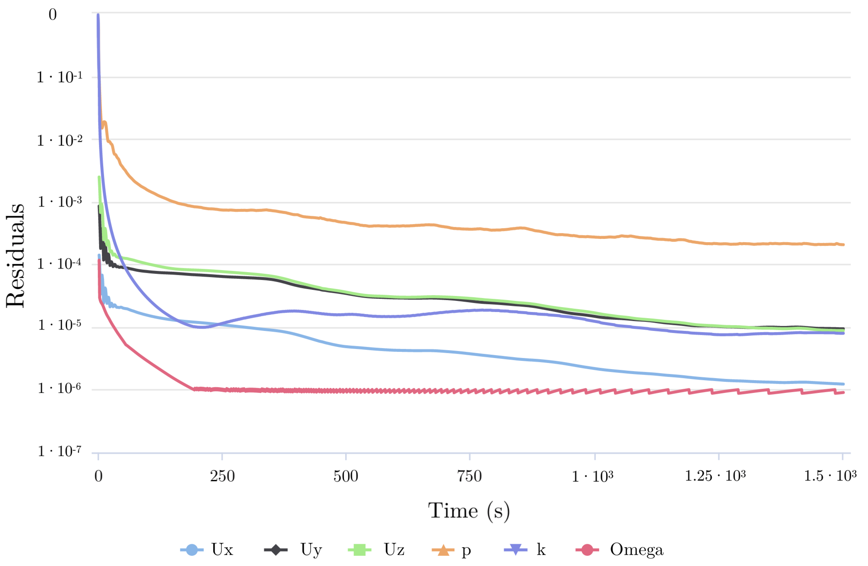
Finally, it was considered to reach convergence when the pressure and velocity residuals were lower than , just as seen in Figure 7. The run time of the cases was around 10 hours under free stream conditions and 17 h under wake flows.
The obtained results are compared with the reference data proposed by Perrin [23], which are obtained through a CFD simulation using TotalSim, a professional enterprise highly experienced in CFD problems. This is taken as a reference as the boundary conditions and the problem definition coincide with the ones that are proposed in this study, although the solvers are different. Besides, reference data have a public background of more than 120 runs evaluated, so this may be considered to be a reliable source of validation.
The numerical prediction deals with the aerodynamic parameters: Downforce (S), Drag (S), overall aerodynamic efficiency E (/), and Front Balance , which is defined as the fraction between the downforce that is generated by the front axle and the total one.
3. Results and Discussion
3.1. Free Stream Condition
Table 3 shows that the results of the performed RANS simulation with k-SST model encounter a notable agreement with the reference data. The error found in both downforce and drag coefficient differs by 4.45% and 6.50%, respectively. This indicates that the overall simulation is acceptable, as the difference between the aerodynamic coefficients is found to be small enough to accept them and validate the reference datum.
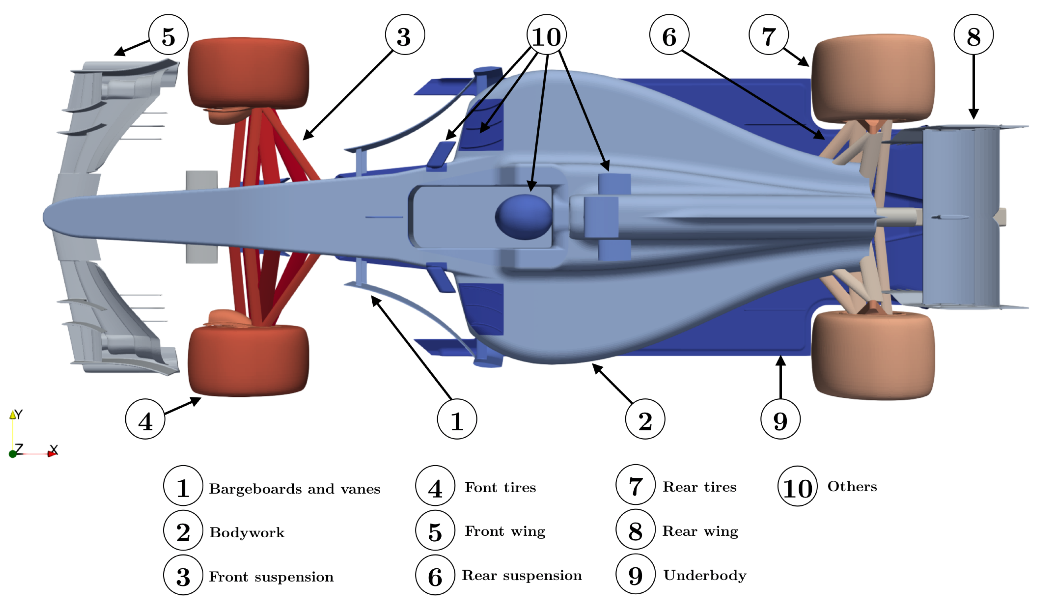
On the other hand, it is found appropriate to indicate the relative contribution in terms of downforce and drag of the main components of the car. This way, it is possible to see the influence of each element and appreciate its aerodynamic efficiency, which is very useful in terms of redesign purposes and issues detection. The different components evaluated can be checked in Figure 8, while Table 4 shows the distribution of these aerodynamic forces.
The underbody, which is composed by the flat floor, the plank, and the diffuser, is responsible for the 60% of the total downforce generation. Following this trend, the rear and the front wing represent, respectively, around 35% and 23% of the overall downforce of the car. The bodywork, shaped as a wing profile, counterbalances these gains by producing lift as well as other elements, such as the front suspension, and both rear and front tires.
On the other hand, Table 4 shows that tires represent around 30% of the total drag, specially on rear’s, as the wheels are not covered. This area is well influenced and dominated by big pressure losses in the wake, which leads to these undesired highly turbulent zones of the total drag of the car. Additionally, the front and the rear wing are also present, by being responsible for 13% and 20% of the total drag, respectively. Other elements, such as the underbody (15% of the drag) and the bodywork (10.70%), take an important contribution regarding the aerodynamic resistance.
In terms of aerodynamic efficiency, it is important to note that the underbody is, with no hesitation, the most efficient part of the car. This can be explained due to the use of Ground effect (despite being limited by the flat floor and the size of the diffuser). As opposed to that, the rear wing is known for its low aspect ratio, which helps to generate big downforce quantities, but it suffers from the production of induced drag. The efficiency of the front wing is somewhere between the underbody and the rear wing: the beneficial points of the rake and ground effect that are commented in [24] are counterbalanced by the high angle of attack of the flaps and the vortices generated at the tips.
Figure 9 shows the pressure distribution by means of the dimensionless coefficient ( around the car, both in terms of a plot and in a three dimensional visualisation. The upper view reflects high-pressure zones that are located in the nose (specially in the front wing) as well the rear wing due to its high curvature. Some stagnation areas are also found around the cockpit, where the pressure distribution is low and smooth. These results are in line with what it was previously commented, with the wings being one of the main generators of downforce due to its high angle of attack and curvature.
On the other hand, the underbody of the car shows low-pressure zones under the wings (as it was clearly expected by its nature and shape). Besides, the low-pressure zones along the floor and diffuser suggest that the car is working properly under the Ground effect. It is possible to see a smooth transition from a medium pressure zone to a low pressure region (meaning that the airflow is being accelerated), and finally an increase of pressure that returns the airflow in a lower velocity to the wake. However, the region in close proximity to the tires is affected by an increase of pressure, which implies the loss of the Ground effect benefits.
In general, the pressure distribution is rather smooth around the car, with no abrupt pressure gradients or unexpected transitions, just like that observed in [4].
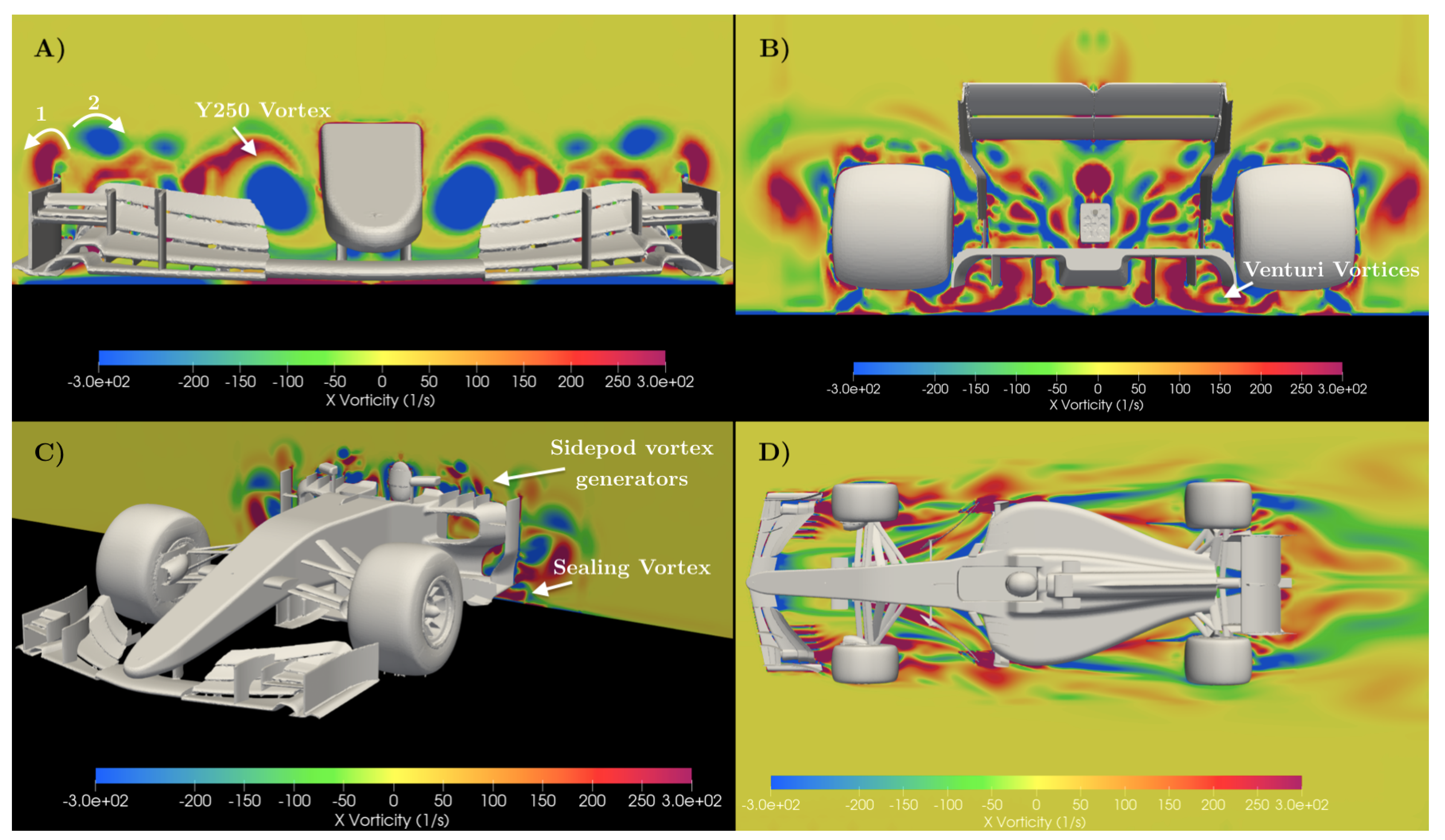
Figure 10 pretends to illustrate to the reader the shape, position and prolongation of some three-dimensional vortical structures, as well as provide several details regarding the strength and rotational axis of such vortices.
Figure 10A shows the multifaceted front wing: not only generating downforce, but also axial vorticity that tends to avoid the front tires and energises the flow downstream. Several vortical structures can be seen on the tip of the endplate (A1) or the winglet endplate (A2), among others. The rotation of the vortices—clockwise or counter clockwise—depends on the pressure field around them [25]. A quite interesting phenomena, as it is clearly the biggest vortex generated in the front wing, is the so-called Y250 vortex. This vortex is developed between the middle section of the wing and the multi flap surface, and it is aimed at recirculating the flow towards the underbody of the car (inwash).
Figure 10B, shows the rear part of the car, where several vortices are originated as a result of the wake of the spinning wheels and other devices. Special attention is placed in the Venturi vortices that are generated on the side of the diffuser due to the pressure gradient between the underbody and the outside. Additionally, the strakes of the diffuser generate small vortices that are coupled with an opposite rotating vortex due to the interaction with the ground boundary layer, similar to the ones observed in [26].
Figure 10C reflects the generation of vortices in the upper middle region of the car. The bargeboards and vanes play a special and important role here. The goal of the latter is to seal and canalise the flow over the bodywork, making sure that the flow keeps attached along the car (Coanda effect). Besides, the sealing vortices that are generated by the bargeboards tend to act as skirts, therefore preventing the underbody airflow to escape and maximise the Ground effect [27] and the diffuser efficiency.
Figure 10D displays a top view of the whole car to understand the behaviour of the overall vorticity.
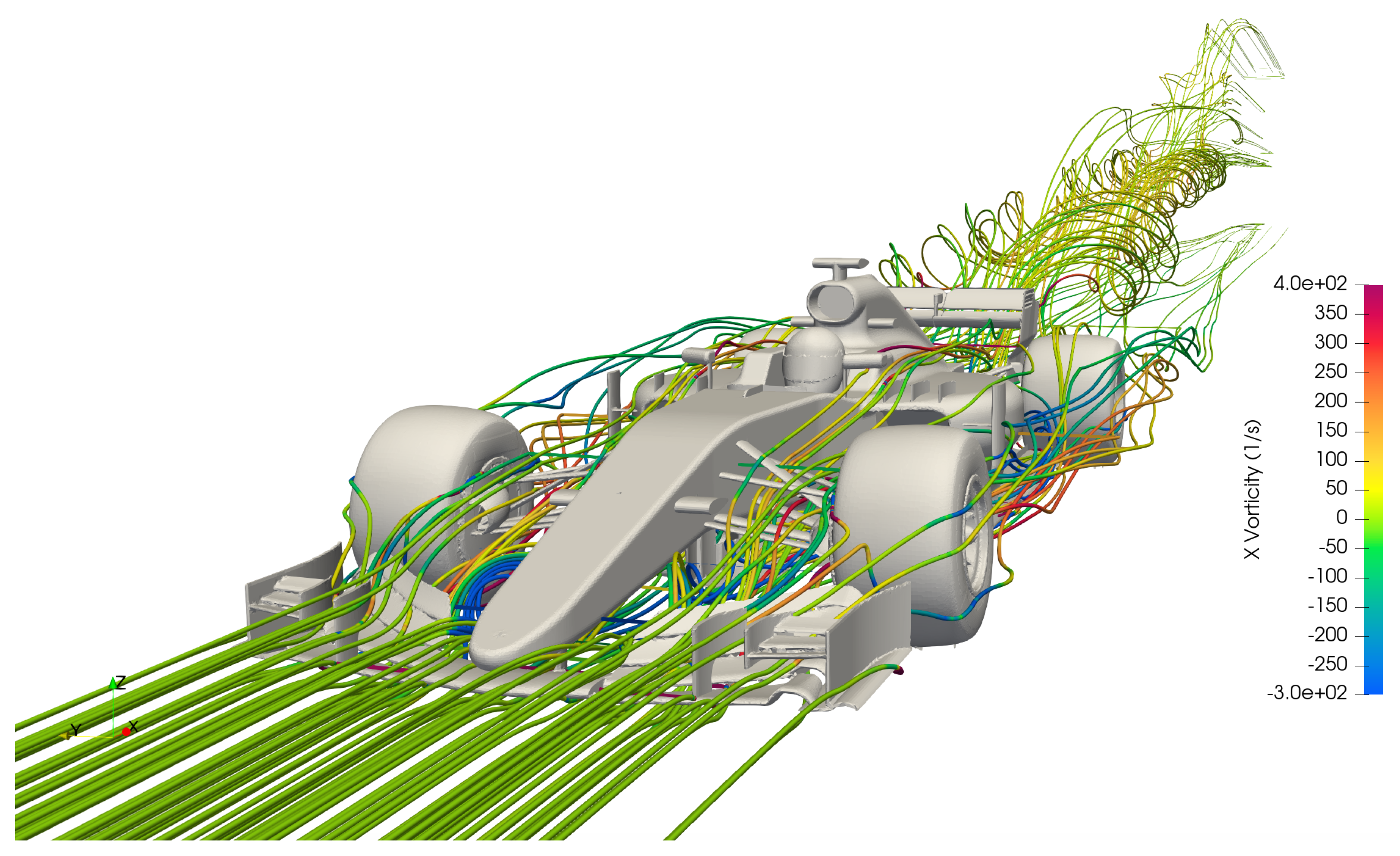
Finally, Figure 11 shows a three dimensional representation of the streamlines of the vorticity. It is possible to see, in general traits, how the flow behaves around different areas of the car (Y250 vortex, tip of the wings, middle section) and how chaotic and turbulent the resulting wake looks like.
3.2. Under Wake flows
Similarly, the evaluated results deal with the aerodynamic parameters: downforce (S), drag (S), overall aerodynamic efficiency E (/), and front balance .
However, four different situations are studied, which differ in the distance established between the 2 cars: 0.25 L, 0.5 L, 1 L, and 2 L, where L represents the length of one car (approximately 5.3 m). Figure 12, Figure 13, Figure 14 and Figure 15 display the evaluated parameters of the second car (follower car) and Table 5 shows the percentage of change of those with respect to the first car (leading car).
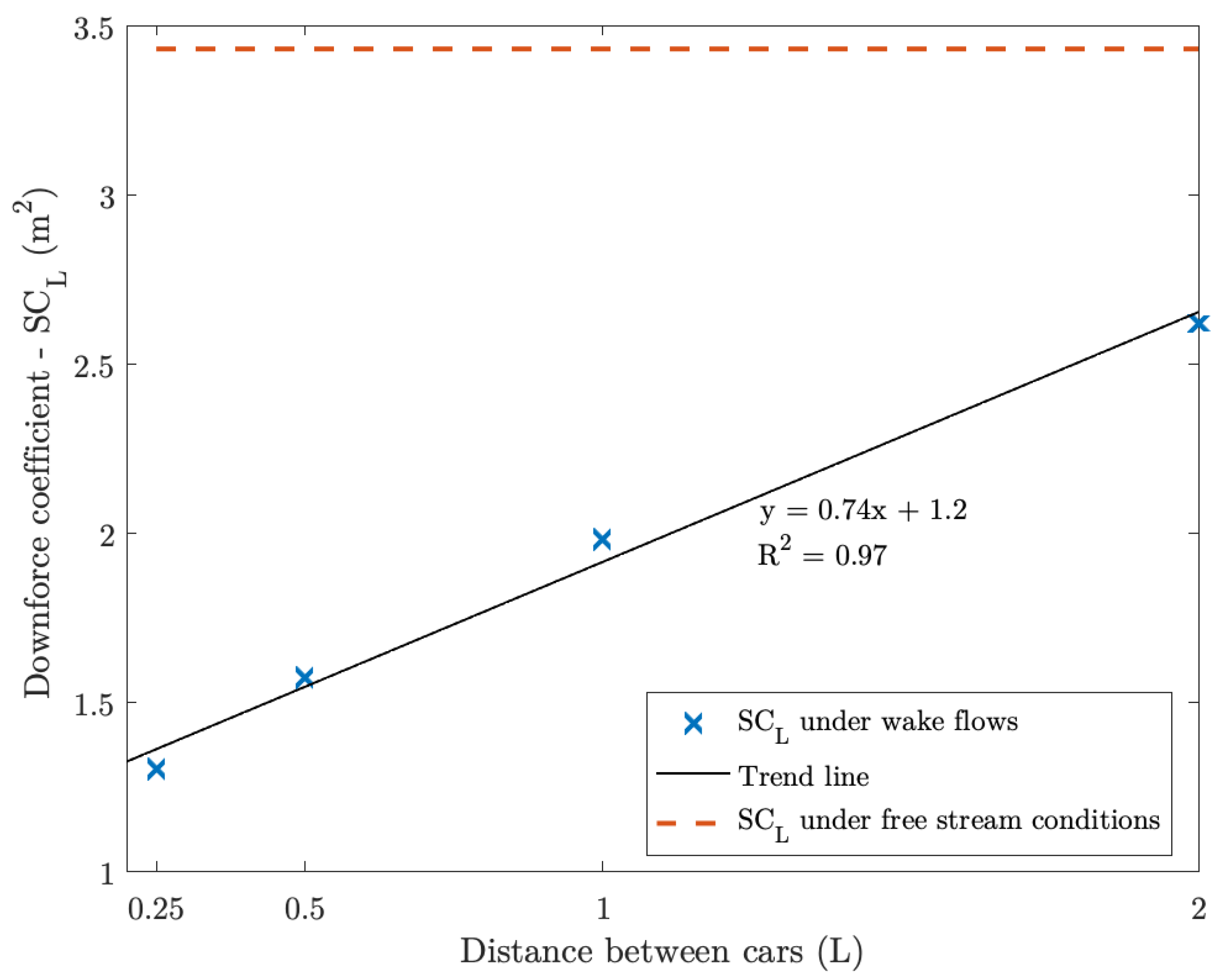
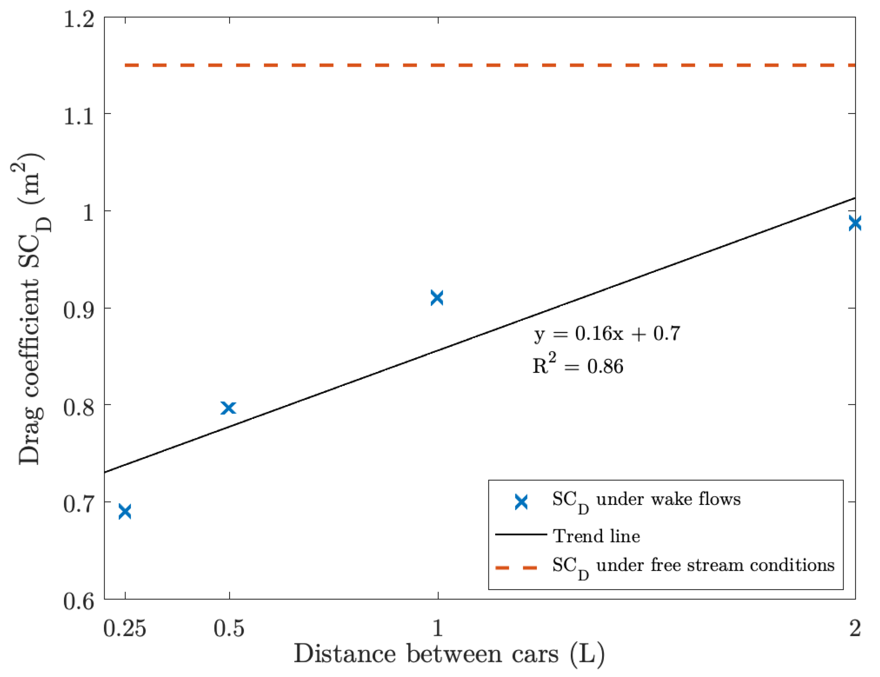
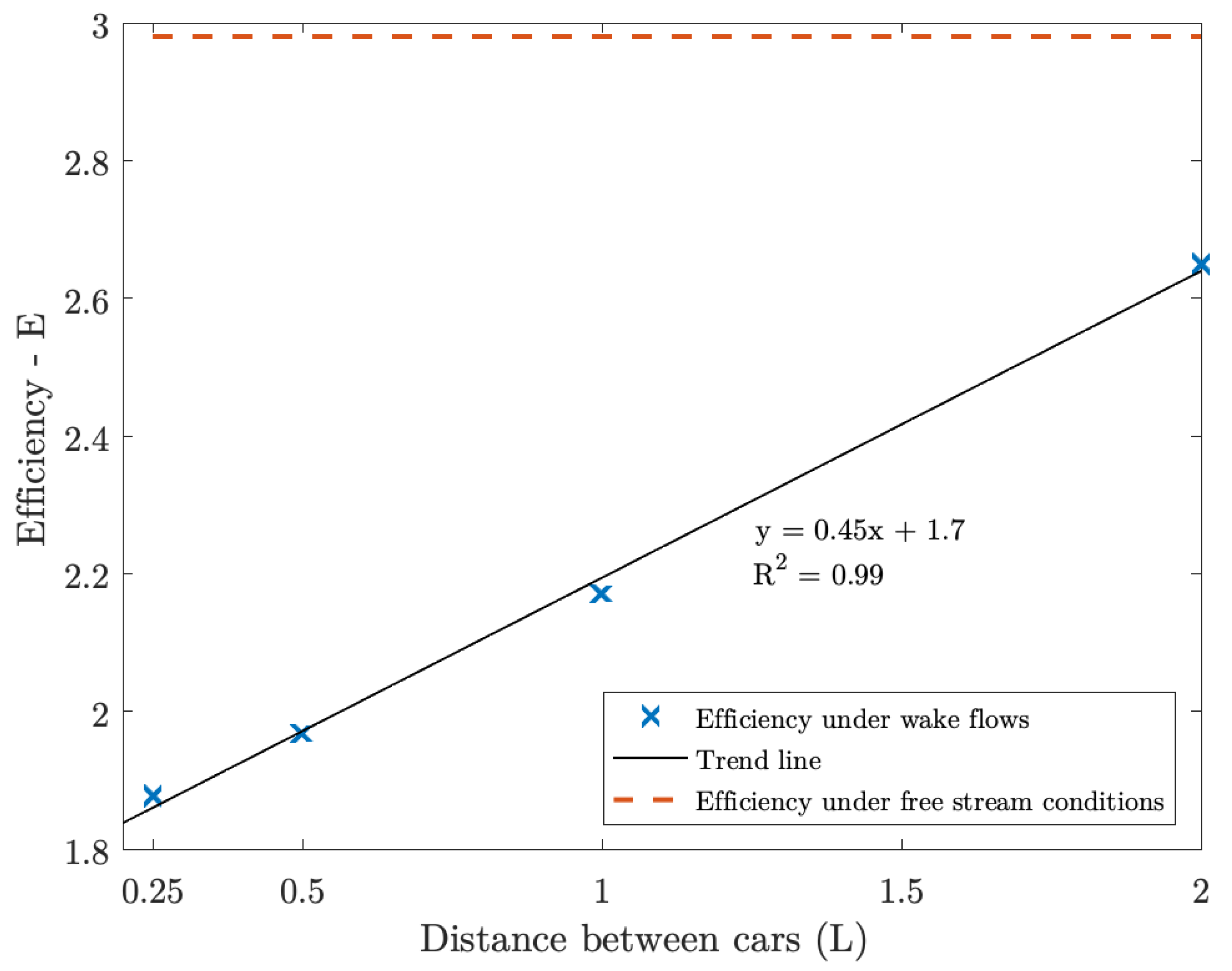
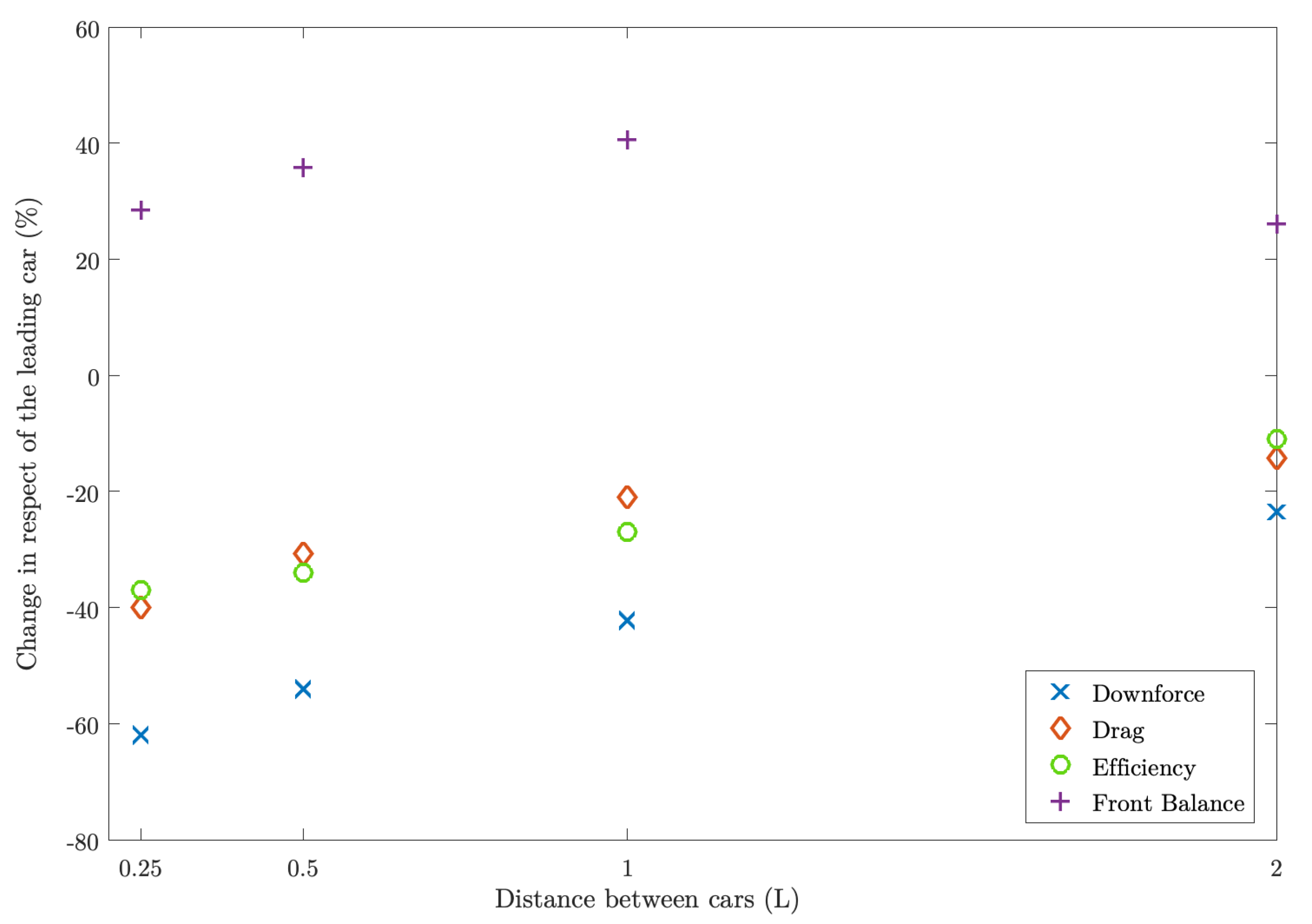
The obtained results show that the reduction in the aerodynamic coefficients is clearly visible from an initial distance of two car lengths (approximately 10.6 m) to the closest case studied of 0.25 L (less than 1.5 m). The reduction of downforce ranges from a −23.5% to a very significant −62% in the worst case scenario. In a similar progression, the drag is reduced from a −14.2% to a −40% and, for this reason, so does the overall efficiency of the second car.
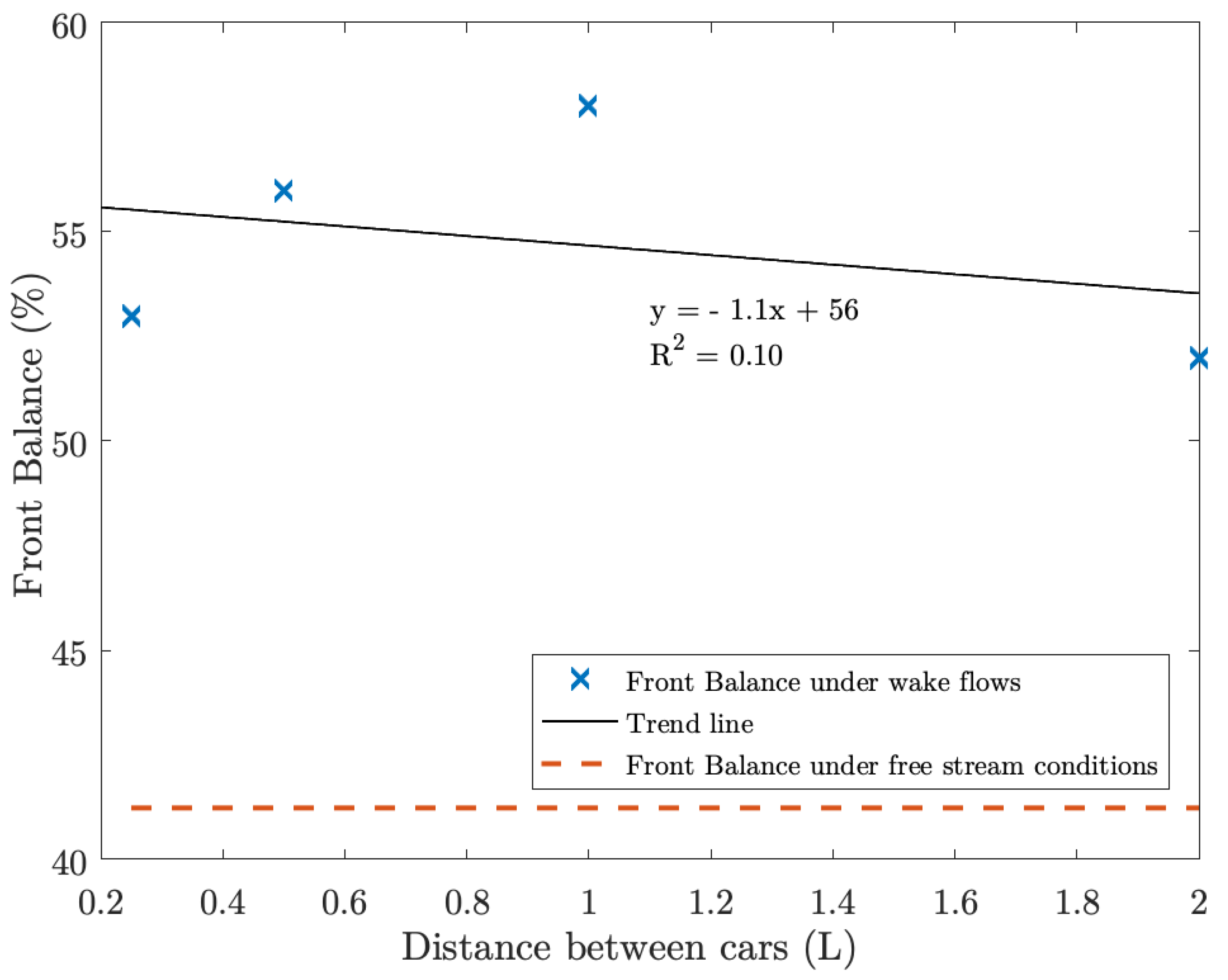
Besides the distinguished loss of downforce, the second car experiences a dramatic increase of front balance (FB) from +26% to 40%. This sudden increase on the front aerodynamic loads may presumably lead to experiencing oversteer (oversteer is caused when a car steers more than intended, thus losing the rear end) and safety issues while braking and on high-speed corners [28].
In general traits, it can be seen that, as the second car approaches and gets closer to the leading one, the aerodynamic loads are reduced, which worsens the performance of the car, but so does the drag. This is energetically a key point, as the power that is required to overcome the drag is smaller when the distance between the cars gets closer, which enables less fuel consumption for the car behind. Table 6 shows a hypothetical situation on the main straight of “Circuit de Barcelona”, Catalunya, where the power and the energy that are required to overcome the different situations are evaluated (it has been assumed a distance of 1 km and a car speed of 50 m/s along the whole straight).
These same conclusions can be easily extrapolated to current road cars, although the conditions and data may differ notably, but not the overall conclusions.
Figure 16 is aimed at showing the obtained data in a visual representation, so that is possible to appreciate the rate of change in the various studied parameters.
As mentioned, the increase of the front balance levels on the second car enables a short, but rather interesting discussion. It is known that the weight distribution of a F1 2017 specification car is around 45.5% on the front axle [29], so the car is not supposed to exceed this 45.5% of front balance, as it may lead to stability concerns. The Center of Pressure, which, by definition, is such where the total sum of pressure fields act on, should always remain behind the Center of Gravity. This can be explained, as the yawing moment of the aerodynamic forces counterbalances the steering of the driver and, therefore, stabilises the car.
On the other hand, if the Center of Pressure is ahead of the Center of Gravity, then the yawing moment increases the sideslip angle and produces instability. As the obtained results show, the front balance of the second car adopts always values that are greater than 45.5% (see Table 5). This implies not only a reduction of the stability and the performance of the car (slower laptimes and more degradation of the front tires), but also a more challenging approach when driving the car; major ease of spinning and safety issues.
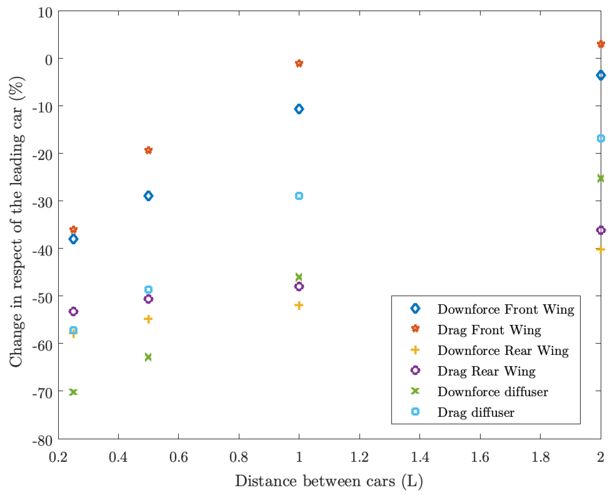
Moreover, the study analyses the performance of the most relevant aerodynamic devices on the follower car: front wing, rear wing, and diffuser.
Table 7 reflects that the loss of downforce of the front wing starts to appear severely at a distance of 1 L up until a very critical −38%, when it reaches 0.25 L. On the other hand, the drag levels are found to be grater than the leading car at a distance of two car lengths, but a similar behaviour to the downforce is found as long as the distance is decreased. This could be explained due to the turbulent conditions that are found far away from the leading car. Moreover, as the second car approaches the leading one, it enters into a very strong wake region that initially hits the front wing and eventually influences all behaviour of the car.
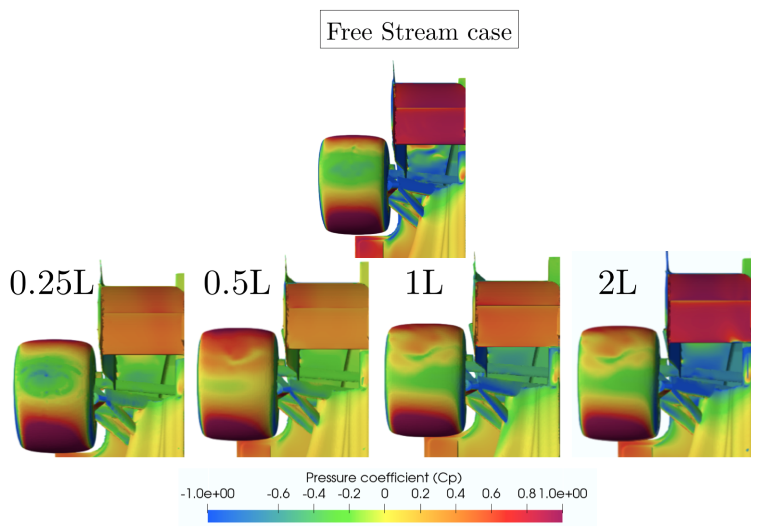
This is precisely seen in Figure 17, where it is possible to see the behaviour commented earlier, as the low pressure zones of the front wing suffer an abrupt change and loss as the car enters into the closer wake region (cases 0.25 L and 0.5 L, where the tendency of the pressure distribution appears slightly inconsistent, although the numerical results do not). It is not at all elementary to try to find a reason why it occurs, but the most sensible explanation lies in the chaotic and unpredictable nature of turbulence. Besides, the larger pressure area located in 0.5 L is found in the very first tip of the front wing, which corresponds to the first element that is encountered by the airflow. In general, these changes are noticeably far less progressive than the rear wing’s, which also evidences the premature front balance shift, but allows a more robust behaviour at greater distances.
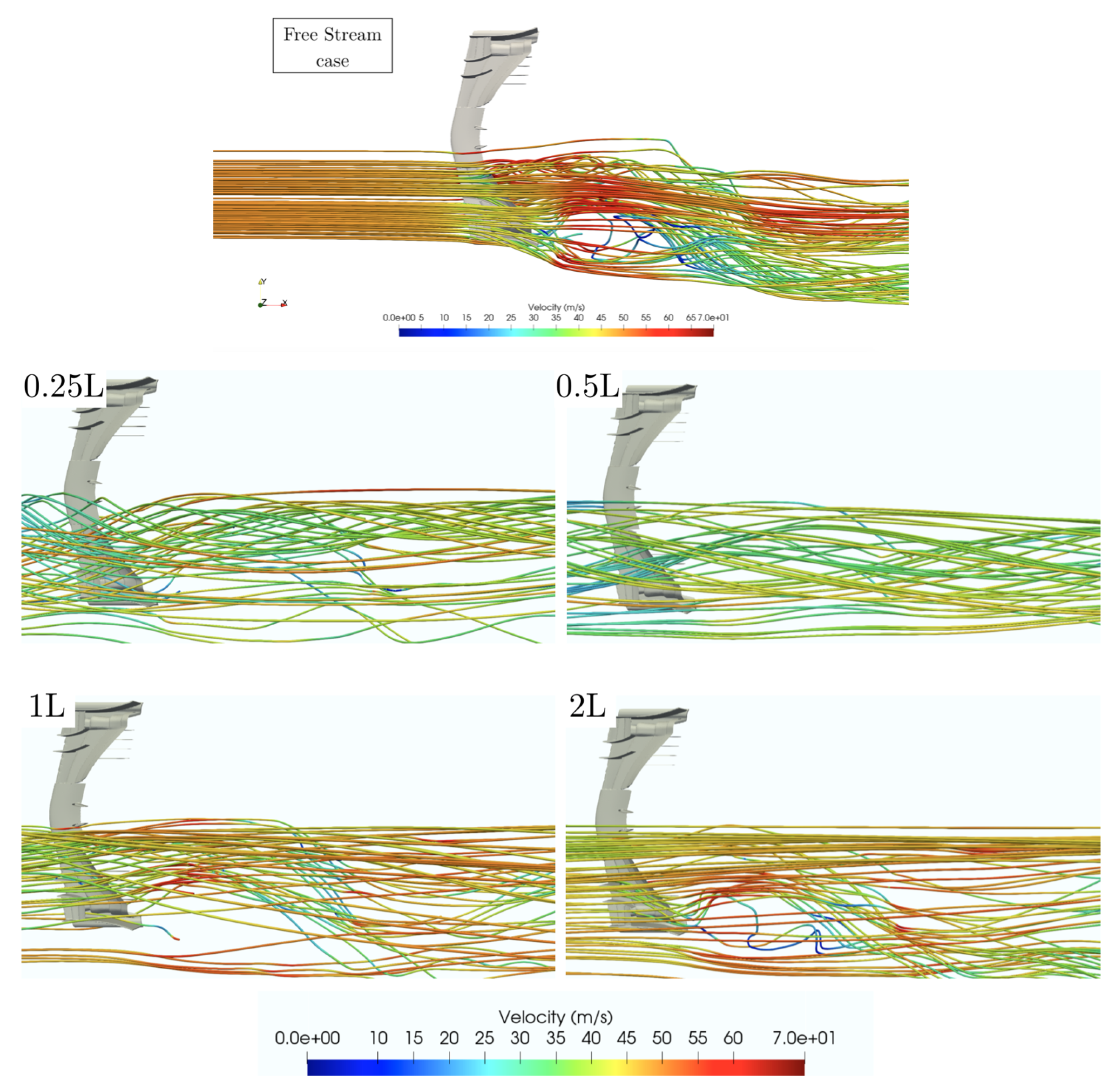
As for the streamlines of the velocity, Figure 18 (2 L) shows that the magnitude of the velocity is somehow similar to the one of the free stream flow, although it presents low velocity areas on the central part of the wing. However, endplates and wing tip elements are still useful for redirecting the flow towards the rear. As the distance is halved, the velocity of the flow is reduced and the front wing loses its capacity to govern the airflow, but it is not until cases 0.5 L and 0.25 L that the front wing is fed by really low kinetic energy flow that leaves it notably inoperative. The effectiveness of the generation of vortices and redirection of the flow is insignificant, just as checked in Table 7 due to the strong wake region.
Shifting to the rear wing, Table 8 portrays that the behaviour of the rear wing is notably different: the loss of downforce is very notable since the very first distance of 2 L and it keeps increasing as the slipstream distance gets closer. Similarly, the drag levels are also strongly reduced from the beginning and matching a comparable ratio that keeps the efficiency almost constant.
It can be stated then, that the rear wing is more affected under the wake effects than the front wing, as the latter seems to suffer less and only under close proximity. This somehow explains the increase of front balance (and forward change of the center of pressure) and its posterior decrease, as sketched in Figure 16.
On the pressure side, from an early stage, one can see that the pressure loss in the rear wing is severely and gradually appreciated. The approach to the leading car distinctly damages the functioning of both its stabilising and suction purposes. Figure 19 sketches these comments.
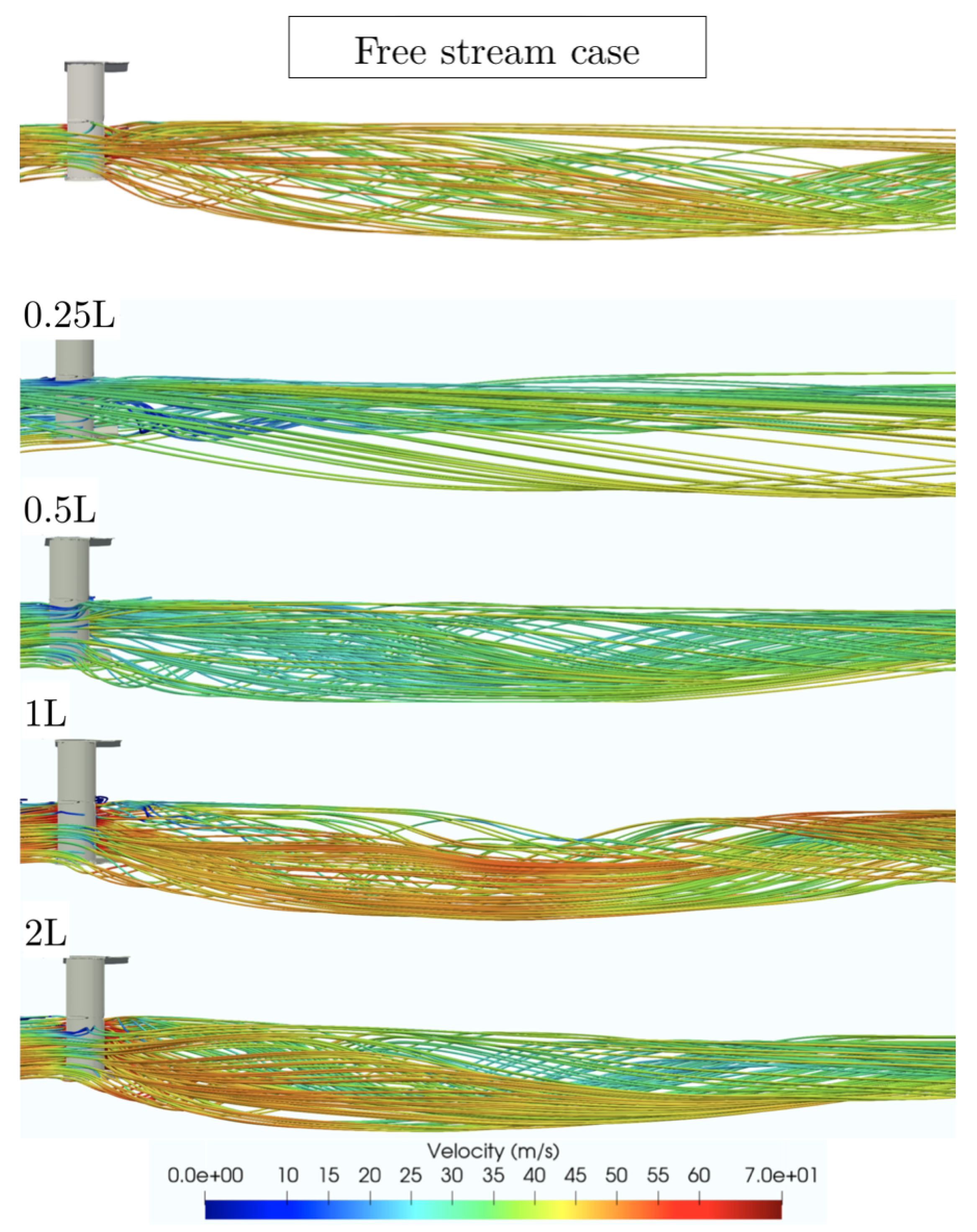
Similarly, under a normal regime, Figure 20 shows that the rear wing works perfectly with aligned flow that is redirected by other aerodynamic devices, but it is possible to see that, as the distance is reduced, the streamlines tend to deflect slightly inboard. The clear jump in terms of velocity magnitude is produced from case 1 L to 0.5 L, where the flow experiences a moderate deceleration as it enters into the strongest wake region. It could be speculated that the rear wing is more sensitive to the direction of the flow than the front wing due to its low aspect ratio, the pronounced curvature, and the massive endplates at both sides. Figure 20 (0.25 L) shows a mixture of velocity flows with very low speed that unexpectedly create an inwash phenomena at the rear end of the wing. This evidences that the whole aerodynamic package of the follower car is prominently disrupted under the wake conditions.
Finally, Table 9 reports that the diffuser is the device that suffers the most under the wake conditions, as the downforce loss that is in close proximity is around 70% and the drag is found to be reduced by around 57% at the same distance. However, the interesting conclusion is that the reduction of downforce starts from the very first beginning and keeps increasing as the distance is reduced.
This evidences that overtaking maneuvers are heavily influenced since the start (it is important not to forget that the diffuser is the greatest source of downforce generation, as seen in Table 4).
This generates an interesting and deep discussion, as it is encountered that the greatest way of generating aerodynamic loads under a free stream flow, is, at the same time, the worst one under wake flows. The whole conception and functioning of the underbody is found to be absolutely pointless; therefore, other aerodynamic paths and solutions should be evaluated if these losses are wished to be recovered.
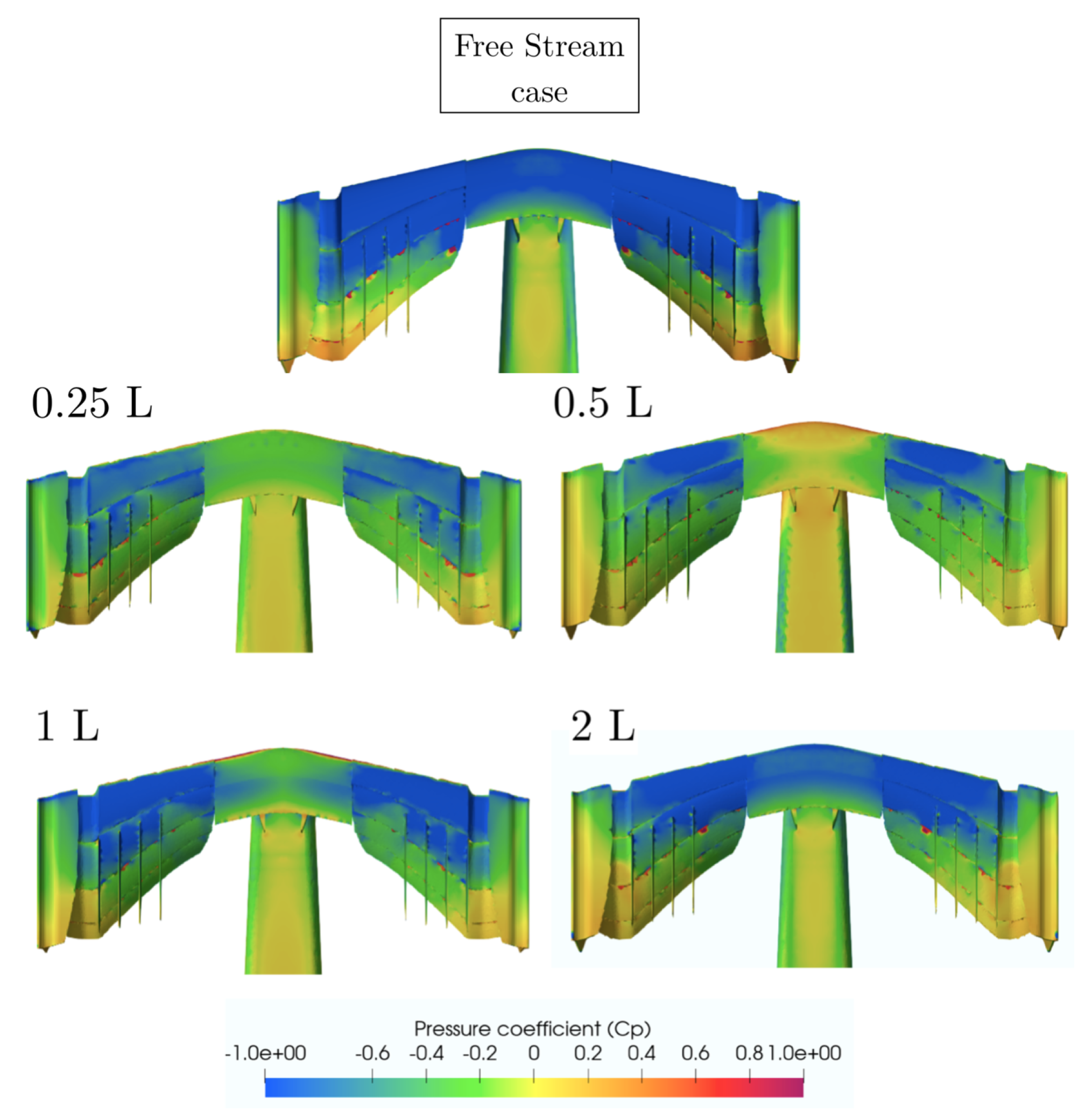
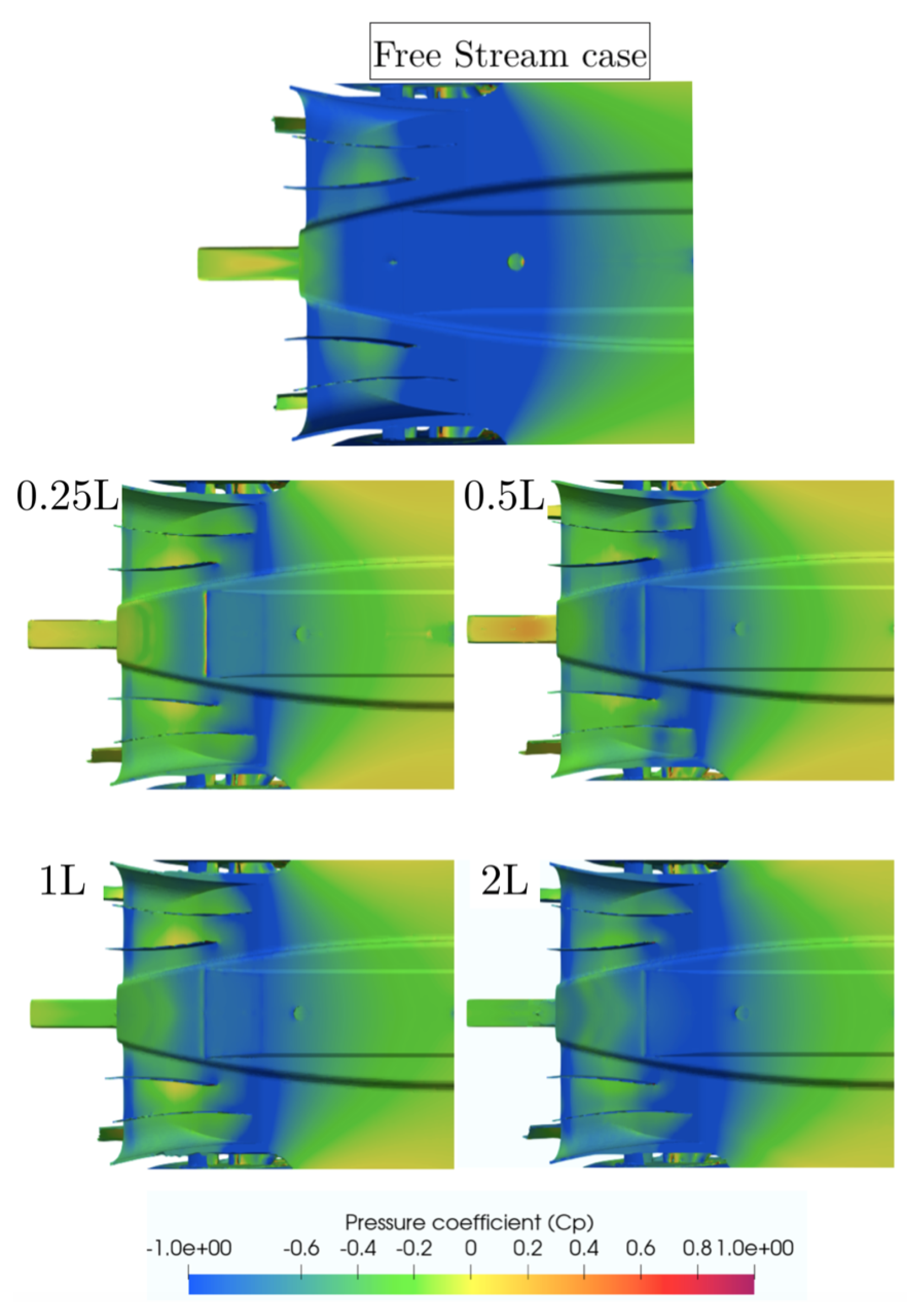
On the pressure side, the results that are presented in Figure 21 again show that the whole low pressure zone is affected since the very first beginning, with moderate areas near the diffuser strakes with higher pressure values. However, the degradation of the performance is perfectly noticeable and again proves that the diffuser suffers excessively under wake flows until its contribution becomes almost negligible.
As for the streamlines of the velocity, Figure 22 describes how the underbody, and particularly the diffuser, is affected by the wake flow. In free stream conditions, the diffuser is fed by a high energised flow that is redirected by the front wing and guided around the flat floor. Nonetheless, the streamlines of the flow are not completely straight, as the vortices management allow for the control of the airflow around the underbody. Figure 22 (2 L) displays a quite non-disturbed behaviour of the airflow, as the management of it is still acceptable. When the distance is reduced, the performance of the underbody starts worsening due to the flow arriving more disturbed into the diffuser, hence not being able to operate properly. Smaller distances, such as cases 0.5 L and 0.25 L, reflect an underbody region that is fed by a very low kinetic and rotational flow.
The main reason for the massive downforce losses that are reported in Table 9 is that the underfloor is notably sensitive under wake flows, as it works closer to the ground than the front wing. This means that the low energy (and highly-rotational) airflow may not be compressed around this small area, therefore experiencing a massive performance loss.
Finally, Figure 23 shows the plots of Table 7, Table 8 and Table 9 in order to appreciate the aforementioned changes in the aerodynamic coefficients of the different elements.
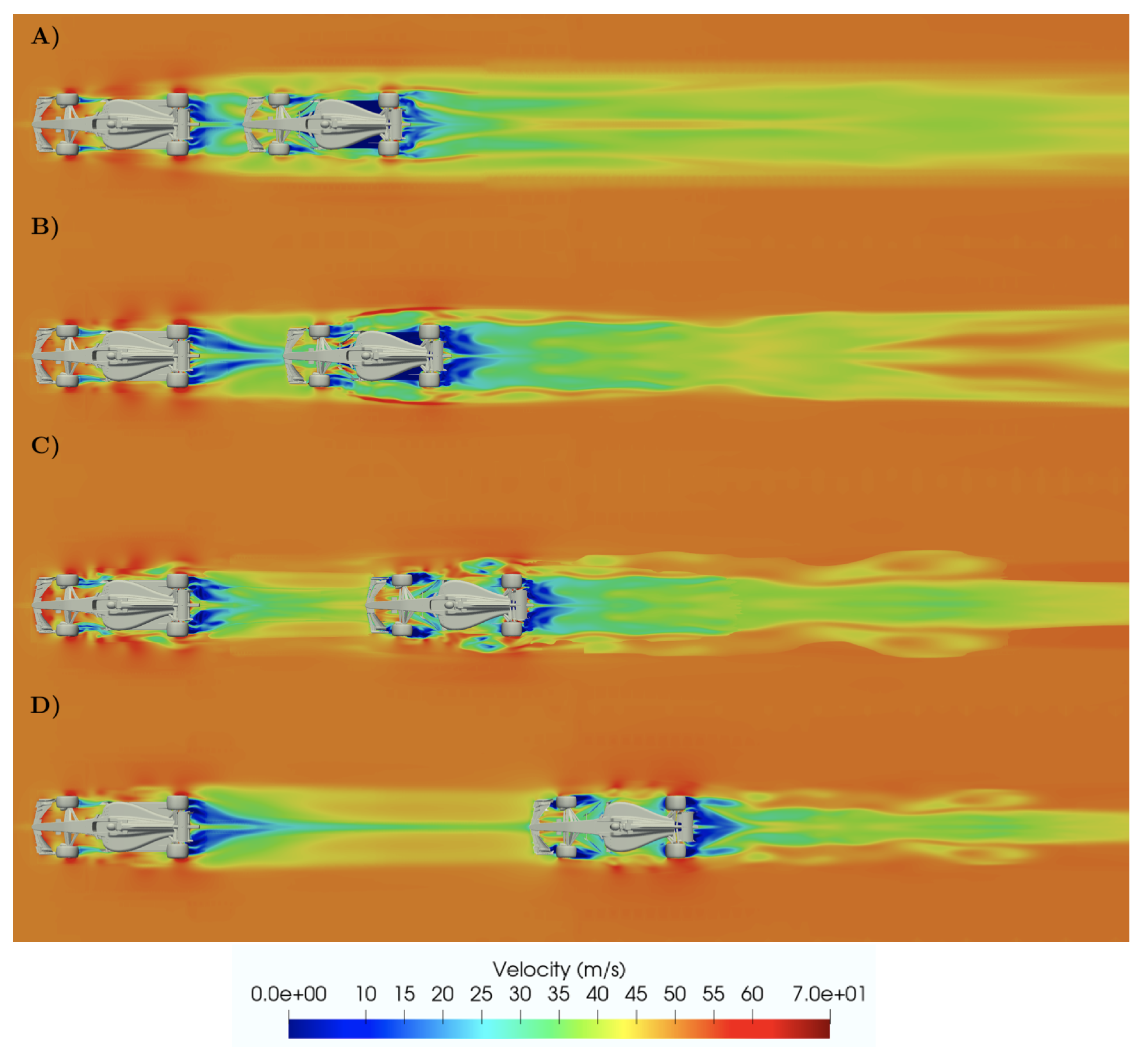
On the wake side, these effects can easily be appreciated in Figure 24, where the second car is affected by a flow that is lower in terms of kinetic energy, as the wake that is generated by the leading car is released far away disturbing its follower. It is also clear that, as the second car gets closer, it inherently enters into a unique wake structure characterised by very low speed flow, that ranges from 0 to 10 m/s, therefore, resulting severely affected. It is seen that as the second car reduces the distance, its wake originates a separation region that enlarges and becomes evident as the distance is closed. At a large distance (2 L), the second car’s wake adopts a needle shape, which somehow imitates the free stream natural wake, but this shape soon disappears at closer distances.
As for the leading car, it can be noted that its wake is not notably modified (in terms of shape and contours) by the presence of the follower car. The aerodynamic coefficients that are evaluated on the leading car only experience a low variation —less than 3%—when the distance between the two cars is set at 0.25 L.
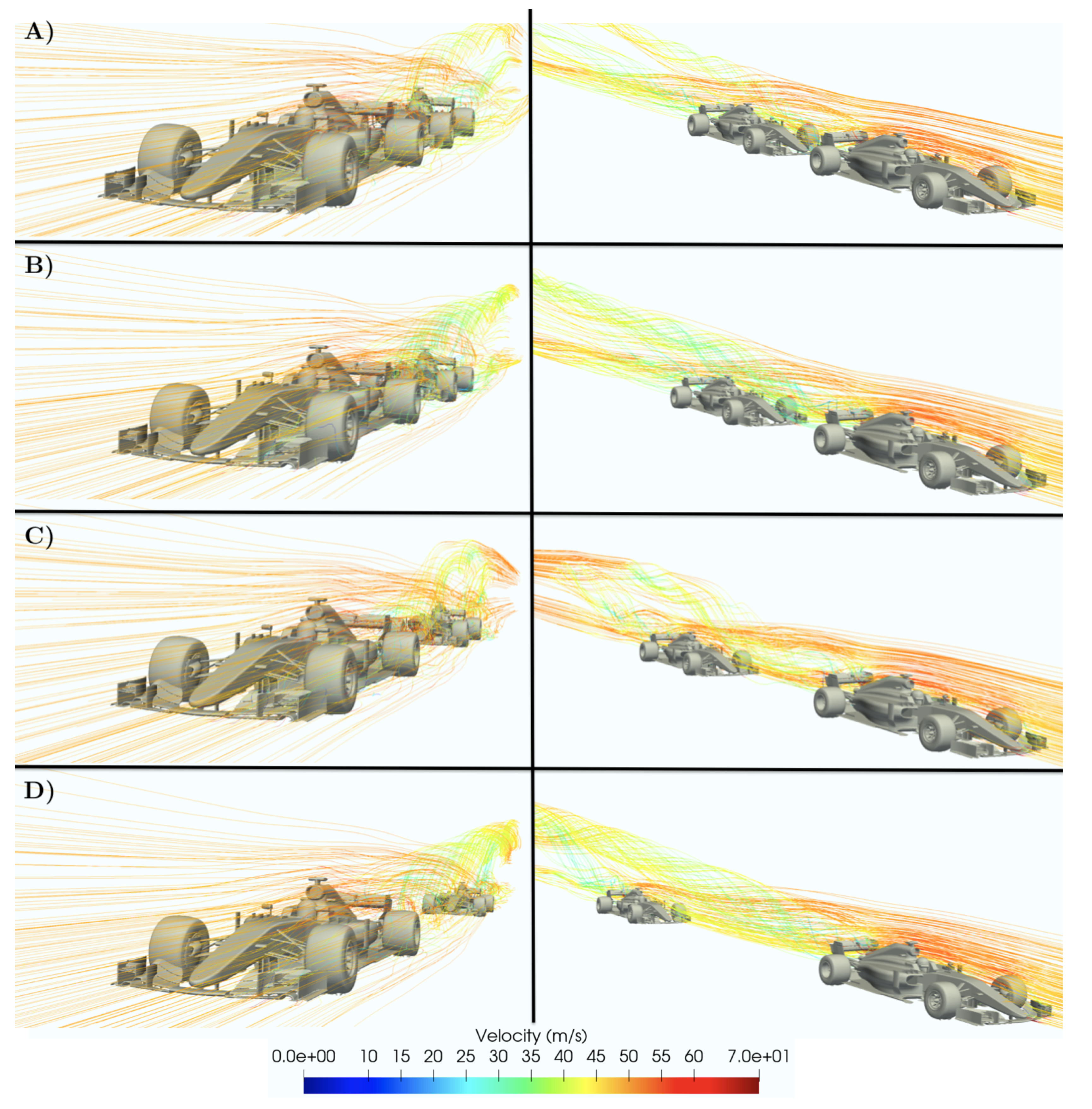
Shifting now to the streamlines of the velocity, Figure 25 displays two different planes for each scenario. The first thing that one may notice is how the airflow is perfectly attached to the first car; from the front wing, going through the sidepods and bodywork and finally exiting the rear wing.
However, it is possible to also see that the exiting airflow on the rear-end of the leading car is somehow divided into two characteristic flows: the first one, located on the superior area, which adopts high-speed values due to being accelerated around the bodywork (low pressure zone and smooth behaviour), and the second one, which exits the diffuser upwards and is mainly a turbulent flow continuously undergoing changes in both magnitude and direction, as reported in [30]. The mixture of the previously mentioned flows is what originates such a chaotic wake region, as it is formed by the combination of multiple flows with various natures and velocities [31].
4. Conclusions
The initial purpose of the present study was to establish whether the current F1 regulations required an urgent aerodynamic change in order to objectively improve the category. In other words, to test and validate, by means of CFD analyses, that the upcoming regulation changes are aerodynamically justified. Accordingly, the results gathered in the present manuscript may be useful to F1 teams, FIA administrations, and to anyone interested in racing aerodynamics.
The obtained results suggest that modern F1 cars are designed and well optimised to run under free stream flows (as the reference data coincides with the numerical results), but they suffer excessively when running under wake flows. Overall, the aerodynamic loads tend to be reduced when running under close proximity, ranging from 23% to a very significant 62% in the closest case.
In regards to the individual focus that is placed on the different aerodynamic devices, it has been found that the front wing experiences a sudden jump on downforce losses only when it enters into the closer wake region. On the other hand, the rear wing massively suffers from long distances, but its losses are way more linear and moderate. As for the diffuser, it is found that it represents the most affected aerodynamic device, as its performance is reduced from a considerable 25% to a huge 70%. This evidences that the conception of the diffuser and vortex management under the floor becomes critically compromised under wake flow conditions.
The modern performance of Ground Effect by means of vortices management represents a very unique and complex way of modelling modern aerodynamics, but, at the same time notably compromise the performance of the cars when an overtaking maneuver is intended. For this reason, it is possible to guarantee that the FIA changes in the current regulations is considered to be adequate, necessary, and justified in terms of aerodynamic necessities.
However, it is essential to comment that the present study presents some research limitations, as CFD methodology always requires an experimental validation. Accordingly, directions in further research point towards experimental validation (involving the use of wind tunnels with movable ground and spinning tires) in order to ensure that the data gathered reflect the reality properly.
Author Contributions
A.G. configured and performed the numerical simulations as well as the analysis of the results and the paper elaboration. R.C. supervised the study and reviewed the final version of the paper. All authors have read and agreed to the published version of the manuscript.
Funding
This research received no external funding.
Conflicts of Interest
The authors declare no conflict of interest.
Abbreviations
The following abbreviations are used in this manuscript:
| CFD | Computational Fluid Dynamics |
| FVM | Finite Volume Method |
| GAMG | Geometric Algebraic Multi Grid |
| GCI | Grid Convergence Index |
| FIA | Federation Internationale de l’Automobile |
| CAD | Computer Aided Design |
| RAM | Random Access Memory |
| L | Vehicle length [m] |
| Reference parameter [] | |
| l | Turbulent length scale [m] |
| I | Turbulent intensity [%] |
| Re | Reynolds Number |
| Cp | Pressure coefficient |
| Fluid density [kg/] | |
| Fluid velocity [m/s] | |
| g | Gravitational acceleration [m/] |
| Dynamic viscosity [kg/m·s] | |
| S | Reference Surface [] |
| Lift coefficient | |
| Drag coefficient | |
| E | Aerodynamic Efficiency |
| FB | Front Balance |
References
- Wilson, M.R.; Dominy, R.G.; Straker, A. The aerodynamic characteristics of a race car wing operating in a wake. SAE Int. J. Passeng. Cars-Mech. Syst. 2008, 1, 552–559. [Google Scholar] [CrossRef]
- Ravelli, U.; Savini, M. Aerodynamic Simulation of a 2017 F1 Car with Open-Source CFD Code. J. Traffic Transp. Eng. 2018, 6. [Google Scholar] [CrossRef]
- Ravelli, U.; Savini, M. Aerodynamic investigation of blunt and slender bodies in ground effect using OpenFOAM. Int. J. Aerodyn. 2019. [Google Scholar] [CrossRef]
- Newbon, J.; Sims-Williams, D.; Dominy, R. Aerodynamic analysis of Grand Prix cars operating in wake flows. SAE Int. J. Passeng. Cars. Mech. Syst. 2017, 10, 318–329. [Google Scholar] [CrossRef] [Green Version]
- Perry, R.; Marshall, D. An Evaluation of Proposed Formula 1 Aerodynamic Regulations Changes Using Computational Fluid Dynamics. In Proceedings of the 26th AIAA Applied Aerodynamics Conference, Honolulu, Hawaii, 18–21 August 2008; p. 6. [Google Scholar] [CrossRef] [Green Version]
- Ogawa, A.; Yano, S.; Mashio, S.; Takiguchi, T.; Nakamura, S.; Shingai, M. Development Methodologies for Formula One Aerodynamics; Honda R&D Technical Review 2009; F1 Special (The third Era Activities): Sakura/Chiba, Japan, 2009. [Google Scholar]
- Senger, S.; Bhardwaj, S.R. Aerodynamic Design of F1 and Normal Cars and Their Effect on Performance. Int. Rev. Appl. Eng. Res. 2014, 2248–9967. [Google Scholar]
- Larsson, T. 2009 Formula One Aerodynamics BMW Sauber F1.09—Fundamentally Different. In Proceedings of the 4th European Automotive Simulation Conference, Munich, Germany, 6–7 July 2009; p. 4. [Google Scholar]
- Reddit. Ferrari SF70H, the 2017 Championship Contender. Available online: https://www.reddit.com/r/formula1/comments/bw9v7z/the_ferrari_sf70h_shark_fin_looks_good/ (accessed on 3 May 2020).
- Newbon, J.; Dominy, R.; Sims-Williams, D. Investigation into the Effect of the Wake from a Generic Formula One Car on a Downstream Vehicle. In Proceedings of the International Vehicle Aerodynamics Conference; Elsevier Science: Amsterdam, The Netherlands, 2014. [Google Scholar]
- Hajdukiewicz, M.; Geron, M.; Keane, M.M. Formal calibration methodology for CFD models of naturally ventilated indoor environments. Build. Environ. 2013, 59, 290–302. [Google Scholar] [CrossRef] [Green Version]
- Williams, J.; Quinlan, W.; Hackett, J.; Thompson, S.; Marinaccio, T.; Robertson, A. A calibration study of CFD for automotive shapes and CD. SAE Trans. 1994, 103, 308–327. [Google Scholar]
- Onshape a PTC Business. Perrinn Limited|Customer. Available online: https://www.onshape.com/customers/perrinn-limited (accessed on 3 May 2020).
- OpenFOAM Foundation. OpenFOAM Resources|Documentation|OpenFOAM. Available online: https://openfoam.org/resources/ (accessed on 2 February 2020).
- Constantin, P.; Foias, C. Navier-Stokes Equations; University of Chicago Press: Chicago, IL, USA, 1988. [Google Scholar]
- Eymard, R.; Gallouët, T.; Herbin, R. Finite volume methods. Handb. Numer. Anal. 2000, 7, 713–1018. [Google Scholar] [CrossRef] [Green Version]
- Menter, F.R.; Kuntz, M.; Langtry, R. Ten years of industrial experience with the SST turbulence model. Turbul. Heat Mass Transf. 2003, 4, 625–632. [Google Scholar]
- Broniszewski, J.; Piechna, J. A fully coupled analysis of unsteady aerodynamics impact on vehicle dynamics during braking. Eng. Appl. Comput. Fluid Mech. 2019, 13, 623–641. [Google Scholar] [CrossRef]
- Moukalled, F.; Mangani, L.; Darwish, M. The Finite Volume Method in Computational Fluid Dynamics; Springer: Berlin/Heidelberg, Germany, 2016; Volume 6. [Google Scholar]
- Celik, I.B.; Ghia, U.; Roache, P.J.; Freitas, C.J.; Coleman, H.; Raad, P.E. Procedure for estimation and reporting of uncertainty due to discretization in CFD applications. J. Fluids Eng. Trans. ASME 2008, 130, 0780011–0780014. [Google Scholar] [CrossRef] [Green Version]
- CFD Online. Turbulence Length Scale-CFD-Wiki, the Free CFD Reference. Available online: https://www.cfd-online.com/Wiki/Turbulence_length_scale (accessed on 1 May 2020).
- CFD Online. Turbulence Intensity-CFD-Wiki, the Free CFD Reference. Available online: https://www.cfd-online.com/Wiki/Turbulence_intensity (accessed on 27 April 2020).
- PERRINN CFD. Available online: https://docs.google.com/spreadsheets/d/1POHSdkdfXeUEeGgh-meufNzVRUycCLvzUfn_TVXs_PE/edit#gid=0 (accessed on 4 March 2020).
- Soso, M.; Wilson, P. Aerodynamics of a wing in ground effect in generic racing car wake flows. Proc. Inst. Mech. Eng. Part D J. Automob. Eng. 2006, 220, 1–13. [Google Scholar] [CrossRef]
- Vargas, R.V. Meteorología Sinóptica—Vorticidad. Available online: https://slideplayer.es/slide/13178976/ (accessed on 9 May 2020).
- Nakagawa, M.; Kallweit, S.; Michaux, F.; Hojo, T. Typical velocity fields and vortical structures around a formula one car, based on experimental investigations using particle image velocimetry. SAE Int. J. Passeng. Cars-Mech. Syst. 2016, 9, 754–771. [Google Scholar] [CrossRef]
- Ehirim, O.; Knowles, K.; Saddington, A. A Review of Ground-Effect Diffuser Aerodynamics. J. Fluids Eng. 2018, 141, 020801. [Google Scholar] [CrossRef]
- Howell, J. Catastrophic lift forces on racing cars. J. Wind. Eng. Ind. Aerodyn. 1981, 9, 145–154. [Google Scholar] [CrossRef]
- McBeath, S. Competition Car Aerodynamics, 3rd ed.; Veloce Publishing: Dorchester/Poundbury, UK, 2017. [Google Scholar]
- Dominy, R. The influence of slipstreaming on the performance of a Grand Prix racing car. Proc. Inst. Mech. Eng. Part D J. Automob. Eng. 1990, 204, 35–40. [Google Scholar] [CrossRef]
- Bleacher Report, Inc. F1 Turbulence: Dumbing It Down|Bleacher Report|. Available online: https://bleacherreport.com/articles/220724-f1-turbulence-dumbing-it-down (accessed on 4 April 2020).
Figure 1.
Ferrari SF70H, a 2017 spec. car. Extracted from Reddit [9].
Figure 1.
Ferrari SF70H, a 2017 spec. car. Extracted from Reddit [9].

Figure 2.
Generic view of the F1 car CAD model used.

Figure 3.
Fluid domain dimensions.

Figure 4.
Overall mesh and refinement enclosures of the free stream case.

Figure 5.
Overall mesh and refinement enclosures under wake effects.

Figure 6.
Mesh (A) front, (B) rear wing, (C) trimetric, and (D) cockpit.

Figure 7.
Residuals of the simulation.

Figure 8.
Evaluated components of a F1.

Figure 9.
Pressure coefficient plot and representation on the upper and under surfaces of the car.

Figure 10.
Several axial vorticity contours: (A) YZ plane at 0.65 m in the X direction, (B) YZ plane at 3.65 m in the X direction, (C) YZ plane at 2.60 m in the X direction, and (D) XY plane at 0 m in the Z direction.
Figure 10.
Several axial vorticity contours: (A) YZ plane at 0.65 m in the X direction, (B) YZ plane at 3.65 m in the X direction, (C) YZ plane at 2.60 m in the X direction, and (D) XY plane at 0 m in the Z direction.

Figure 11.
Streamlines of the axial vorticity.

Figure 12.
Comparison between values of S under wake flows and under free stream conditions.

Figure 13.
Comparison between values of S under wake flows and under free stream conditions.

Figure 14.
Comparison between values of efficiency under wake flows and under free stream conditions.
Figure 14.
Comparison between values of efficiency under wake flows and under free stream conditions.

Figure 15.
Comparison between values of front balance under wake flows and under free stream conditions.
Figure 15.
Comparison between values of front balance under wake flows and under free stream conditions.

Figure 16.
Percentage change of the performance of the second car in respect of the leading car.

Figure 17.
Pressure coefficient distribution on the front wing of the second car at a distance of 0.25 L, 0.5 L, 1 L, and 2 L as compared to the free stream case.
Figure 17.
Pressure coefficient distribution on the front wing of the second car at a distance of 0.25 L, 0.5 L, 1 L, and 2 L as compared to the free stream case.

Figure 18.
Streamlines of the velocity. Front wing of the second car at a distance of 0.25 L, 0.5 L, 1 L, and 2 L as compared to the free stream case.
Figure 18.
Streamlines of the velocity. Front wing of the second car at a distance of 0.25 L, 0.5 L, 1 L, and 2 L as compared to the free stream case.

Figure 19.
Pressure coefficient distribution on the rear wing of the second car at a distance of 0.25 L, 0.5 L, 1 L, and 2 L as compared to the free stream case.
Figure 19.
Pressure coefficient distribution on the rear wing of the second car at a distance of 0.25 L, 0.5 L, 1 L, and 2 L as compared to the free stream case.

Figure 20.
Streamlines of the velocity. Rear wing of the second car at a distance of 0.25 L, 0.5 L, 1 L, and 2 L as compared to the free stream case.
Figure 20.
Streamlines of the velocity. Rear wing of the second car at a distance of 0.25 L, 0.5 L, 1 L, and 2 L as compared to the free stream case.

Figure 21.
Pressure coefficient distribution on the diffuser of the second car at a distance of 0.25 L, 0.5 L, 1 L, and 2 L as compared to the free stream case.
Figure 21.
Pressure coefficient distribution on the diffuser of the second car at a distance of 0.25 L, 0.5 L, 1 L, and 2 L as compared to the free stream case.

Figure 22.
Streamlines of the velocity. Diffuser of the second car at a distance of 0.25 L, 0.5 L, 1 L, and 2 L as compared to the free stream case.
Figure 22.
Streamlines of the velocity. Diffuser of the second car at a distance of 0.25 L, 0.5 L, 1 L, and 2 L as compared to the free stream case.

Figure 23.
Percentage of change on the performance of the second car.

Figure 24.
Velocity contours on a top plane at a distance of (A) 0.25 L, (B) 0.5 L, (C) 1 L, and (D) 2 L.
Figure 24.
Velocity contours on a top plane at a distance of (A) 0.25 L, (B) 0.5 L, (C) 1 L, and (D) 2 L.

Figure 25.
Streamlines of the velocity at a distance of (A) 0.25 L, (B) 0.5 L, (C) 1 L, and (D) 2 L.
Figure 25.
Streamlines of the velocity at a distance of (A) 0.25 L, (B) 0.5 L, (C) 1 L, and (D) 2 L.


Table 1.
Grid Convergence Index result of the meshes studied.
| Mesh Parameters | = S· |
|---|---|
| Number of elements N1, N2, N3 | 18055055, 13793013, 10634551 |
| Refinement ratio | 1.309 |
| Refinement ratio | 1.297 |
| Finest result | −3.43 |
| Intermediate result | −3.40 |
| Coarsest result | −3.28 |
| Order of convergence p | 4.37 |
| Error | 1.1% |
| Error | 3.7% |
Table 2.
Setup of the simulation.
| Variable | Value |
|---|---|
| Free stream velocity | 50 m/s |
| Fluid density () | 1.225 kg/ |
| Turbulent Intensity (I) [22] | 0.15% |
| Turbulent length scale (l) | 3.475 m |
| Reynolds Number (Re) |
Table 3.
Comparison between the simulation and reference data.
| S () | S () | |/| | FB (%) | |
|---|---|---|---|---|
| Reference Data | −3.59 | 1.23 | 2.92 | 44.80 |
| Simulation Results | −3.43 | 1.15 | 2.98 | 41.23 |
| Error (%) | 4.45 | 6.50 | 2.15 | 7.97 |
Table 4.
Relative downforce and drag contributions of the different elements.
| Elements | Downforce Contribution (%) | Drag Contribution (%) |
|---|---|---|
| Bargeboards and vanes | −1.71 | +2.97 |
| Bodywork | +21.10 | +10.7 |
| Front suspension | +2.36 | +2.88 |
| Front Tires | +2.94 | +10.30 |
| Front Wing | −22.84 | +12.69 |
| Rear suspension | −0.40 | +3.93 |
| Rear tires | +1.42 | +20.06 |
| Rear wing | −35.46 | +20.38 |
| Underbody | −61.09 | +15.05 |
| Others | −6.65 | +1 |
Table 5.
Percentage of change of the aerodynamic coefficients of the second car as regards the first car.
Table 5.
Percentage of change of the aerodynamic coefficients of the second car as regards the first car.
| Distance | S () | S () | |/| | FB |
|---|---|---|---|---|
| 0.25 L | −62% | −40% | −37% | +28.5% |
| 0.5 L | −54.1% | −30.7% | −34% | +35.8% |
| 1 L | −42.3% | −21% | −27% | +40.7% |
| 2 L | −23.5% | −14.2% | −11% | +26.1% |
Table 6.
Energetic parameters required to overcome the air resistance.
| Distance | Power Required (kW) | Energy Required (kJ) |
|---|---|---|
| 0.25 L | 33.44 | 668.8 |
| 0.5 L | 40.39 | 807.84 |
| 1 L | 50.77 | 1015.52 |
| 2 L | 67.32 | 1346.4 |
| Free stream | 88 | 1760 |
Table 7.
Percentage of change of the aerodynamic coefficients in the front wing of the second car as regards the first car.
Table 7.
Percentage of change of the aerodynamic coefficients in the front wing of the second car as regards the first car.
| Distance Front Wing | S () | S () |
|---|---|---|
| 0.25 L | −38% | −36.1% |
| 0.5 L | −29% | −19.3% |
| 1 L | −10.7% | −1.1% |
| 2 L | −3.6% | +3% |
Table 8.
Percentage of change of the aerodynamic coefficients in the rear wing of the second car as regards the first car.
Table 8.
Percentage of change of the aerodynamic coefficients in the rear wing of the second car as regards the first car.
| Distance Rear Wing | S () | S () |
|---|---|---|
| 0.25 L | −57.9% | −53.3% |
| 0.5 L | −54.8% | −50.6% |
| 1 L | −52% | −48% |
| 2 L | −40.3% | −36.2% |
Table 9.
Percentage of change of the aerodynamic coefficients in the diffuser of the second car as regards the first car.
Table 9.
Percentage of change of the aerodynamic coefficients in the diffuser of the second car as regards the first car.
| Distance Diffuser | S () | S () |
|---|---|---|
| 0.25 L | −70.2% | −57.2% |
| 0.5 L | −62.8% | −48.7% |
| 1 L | −46.1% | −29% |
| 2 L | −25.3% | −16.9% |
© 2020 by the authors. Licensee MDPI, Basel, Switzerland. This article is an open access article distributed under the terms and conditions of the Creative Commons Attribution (CC BY) license (http://creativecommons.org/licenses/by/4.0/).
Share and Cite
MDPI and ACS Style
Guerrero, A.; Castilla, R. Aerodynamic Study of the Wake Effects on a Formula 1 Car. Energies 2020, 13, 5183. https://0-doi-org.brum.beds.ac.uk/10.3390/en13195183
AMA Style
Guerrero A, Castilla R. Aerodynamic Study of the Wake Effects on a Formula 1 Car. Energies. 2020; 13(19):5183. https://0-doi-org.brum.beds.ac.uk/10.3390/en13195183
Chicago/Turabian StyleGuerrero, Alex, and Robert Castilla. 2020. "Aerodynamic Study of the Wake Effects on a Formula 1 Car" Energies 13, no. 19: 5183. https://0-doi-org.brum.beds.ac.uk/10.3390/en13195183
Note that from the first issue of 2016, this journal uses article numbers instead of page numbers. See further details here.