Conditional-Robust-Profit-Based Optimization Model for Electricity Retailers with Shiftable Demand

Abstract

This paper investigates the problem of how to deploy customers’ shiftable load (SL) for electricity retailers’ risk management under uncertainty of the day-ahead (DA) wholesale market price. The robust profit (RP) and the conditional robust profit (CRP) are introduced for a risk-averse retailer’s risk-reward trade-off analysis in its decision-making of electricity procurement from various options. A CRP-based bi-level optimization model is proposed for the risk-averse retailer to determine its electricity procurement strategy taking into consideration customers’ shiftable load. In the upper problem, the retailer decides its electricity procurement from various options and the SL incentive prices to maximize its CRP under a given confidence level, and in the lower problem, the customers shift their load according to the SL incentive prices to minimize their comprehensive costs including the discomfort cost caused by rescheduling electricity consumption. Finally, a case study is used to verify the effectiveness of this model. It is shown that the retailer can achieve larger profit and less risk by utilizing customers’ SL and the retailer’s risk-aversion level has an important impact on its electricity procurement and SL incentive strategies.

1. Introduction

1.1. Background

In the deregulated electricity market, retailers can acquire electricity through various options, e.g., the day-ahead (DA) wholesale market, bilateral contracts and self-owned distributed generation (DG). Due to the high volatility of the DA market prices [1], retailers need to adopt risk management methods to mitigate the risk arising from market price uncertainty. In addition, with the rapid development of smart grid technologies around the world, customers’ demand response (DR) has received massive attentions and applications. DR programs (DRP) can be classified into two main categories: price-based DRP and incentive-based DRP [2,3]. Specifically, in the price-based DRP, such as time-of-use (TOU) pricing [4] and real time pricing(RTP) [5], customers adjust their demand in response to price changes over time. In the incentive-based DRP, e.g., direct load control, interruptible load (IL), demand bidding and emergency DR, appropriate incentive payments should be given to customers for their participation in the programs [2]. It is recognized that retailers can deploy their customers’ DR capability to manage risk caused by the uncertainty of the DA wholesale market prices [6]. To this end, investigating electricity procurement strategy from various options for retailers with DR capability is of great importance, especially when the DA market price uncertainty is considered.

Risk management has been one of the main concerns of decision makers for many years [7]. As most of decisions to be made are subject to uncertainties, various risk management methods are applied in different areas of the power system such as power distribution operation [8], transmission planning [9] and electricity market [10]. Risk management is one of the most valuable tasks for electricity sector decision makers to protect their benefit while confronting the uncertainties in price, availability of transmission lines and many other factors. Besides, the study results shown in [11] suggest that adopting integrated and comprehensive risk management systems can help non-financial firms such as companies in the electricity sector, to gain a higher firm value.

1.2. Literature Review

Different risk management methods for electricity retailers’ decision-making under uncertainty have been proposed in the literature. According to how uncertain parameters are considered, methods of risk management can be divided into two categories: probabilistic methods and non-probabilistic methods. The decision-making with probabilistic methods is commonly based on risk–reward trade-off analysis when the probability distribution function of uncertain data is known [12]. In such a type of analysis, the risk is quantified by a measure of the loss such as the value-at-risk (VaR) [13] or the conditional value-at-risk (CVaR) [14,15]. In [13], the VaR method is used to determine a retailer’s optimal electricity portfolio strategy under uncertain market price and demand. However, the VaR is only coherent when underlying risk factors are normally distributed and suffers from being intractable when it is calculated using scenarios [16]. Futhermore, the VaR does not indicate the extent of the losses that might be suffered beyond the amount indicated by this measure [17]. The CVaR is an alternative measure to the VaR that provides an estimate of the losses that might be encountered in the tail [17]. It is also considered as a more consistent measure of risk than the VaR [18]. In [14], the problem of designing retailers’ customized pricing strategies for customers is investigated while the CVaR is used to quantify the risk caused by the price fluctuations of the DA and real-time markets.

Non-probabilistic methods are adopted when the uncertain parameters are under severe uncertainty. The robust optimization (RO) is a modeling framework for immunizing against data uncertainties in which we optimize against the worst case that might arises with a min-max objective [19]. The RO does not require specific probability distribution of the uncertain parameter, instead, the uncertain parameter is characterized by an uncertainty set, e.g., box uncertainty set, ellipsoidal uncertainty set and polyhedral uncertainty set. In [20], the robust optimal bidding and offering strategy in the DA market by a retailer is obtained while the polyhedral uncertainty set is used to describe the uncertainty in the DA market prices. Ref. [21] proposes a robust self-scheduling model for power generators while the uncertainty of electricity price is described by the ellipsoidal uncertainty set. However, with different uncertainty sets selected, the RO model may lead to over-conservatism or computational intractability [22]. The information gap decision theory (IGDT) is another widely used non-probabilistic risk management approach that doesn’t need much data for uncertainty modeling. In addition, with two immunity functions namely robustness and opportunity functions, the IGDT informs the decision makers about the negative and positive outcomes resulted from uncertainties so that they can take appropriate decisions that may be safe or risky [23]. In [24], the IGDT method is used to obtain retailers’ optimal bidding and offering curves in the wholesale market in the presence of market price uncertainty. In [25], a robust bi-level decision-making framework for retailers to supply electricity to price-sensitive customers is presented while the IGDT approach is used to evaluate the financial risk arising from uncertain wholesale prices. The main limitation of the IGDT method is that it also suffers from being over-conservative and the degree of conservativeness cannot be controlled by the decision makers [26].

Recently, increasing attention has been devoted to the development of decision-making strategies for electricity retailers taking DRPs into consideration. In [27], the energy procurement and TOU pricing strategies of a retailer are specified while the RO method is used for risk menagement under spot market price uncertainty. In [28], a two-stage two-level model for the energy pricing and procurement problem faced by a retailer is proposed. Specifically, consumers’ DR with respect to the RTP is characterized by a two-level model in the first stage. In the second stage, risk-averse energy procurement of the retailer accounting for market price uncertainty is modeled by a linear RO. In [29], a multi-objective model for a retailer with IL capability is proposed to maximize the retailer’s profit and minimize the peak demand while the uncertainties of market prices and demand are not considered. In [30,31], stochastic optimization models for retailers with reward-based load-reduction DR are proposed while the CVaR is adopted for risk measurement. It is shown that retailers can avoid unfavorable prices in the real-time market and amend imbalances in demand by participating in the reward-based DRP. Retailers’ energy allocation in the wholesale market, contracts market and short-term DR bidding market is investigated in [32] based on the RO to minimize the electricity procurement cost. In [33], a CVaR-based bi-level optimization model for retailers’ trading strategy with multi-segment IL contracts offered to customers is developed. The proposed strategy can help retailers to gain more market share and enhance their competitiveness.

To date, most of the research on retailers’ risk-based decision-making with consideration of the incentive-based DRPs focus on specifying retailers’ DR incentive strategies for customers’ IL. Besides the IL, the shiftable load (SL) is another important DR resource that plays an increasing role in demand side management [34,35]. In addition, simulation results based on historic data in [36] show that shifting customers’ load demand from peak to off-peak periods can reduce retailers’ expenditures and their fluctuations. The SL resources are scheduled by retailers with time varying prices in most literature [14,37]. In [38], the problem of load-shifting in smart grid is formulated as a Stackelberg game in which the energy provider offers price discounts to motivate customers to shift their load from peak periods, but the uncertainty of market prices is neglected. From above literature review we notice that, very few studies address the problem of how to deploy customers’ incentive-based SL for retailers’ risk management in electricity procurement from various options.

1.3. Layout of the Paper

To bridge the gaps of existing research, the problem of how to deploy customers’ incentive-based SL for retailers’ risk management under uncertain DA wholesale market prices is investigated in this paper. The robust profit (RP) and the conditional robust profit (CRP) [39] are introduced for a risk-averse retailer’s profit-risk trade-off analysis in its decision-making of electricity procurement from various options. Then a CRP-based bi-level optimization model is proposed for a risk-averse retailer to determine its electricity procurement strategy taking into consideration customers’ incentive-based SL capability. The bi-level optimization model is reformulated into a mixed-integer nonlinear programming problem. The effectiveness of the model is verified by a case study. The impacts of customers’ load-shifting capability and the retailer’s risk aversion level are also investigated.

The rest of this paper is organized as follows: Section 2 introduces the concepts and formulation of the RP and CRP. The CRP-based bi-level model for a risk-averse retailer with incentive-based SL considering uncertain DA market prices is formulated in Section 3. Simulation results of a case study are presented in Section 4. Finally, conclusions are drawn in Section 5.

2. Concepts and Formulation of RP and CRP

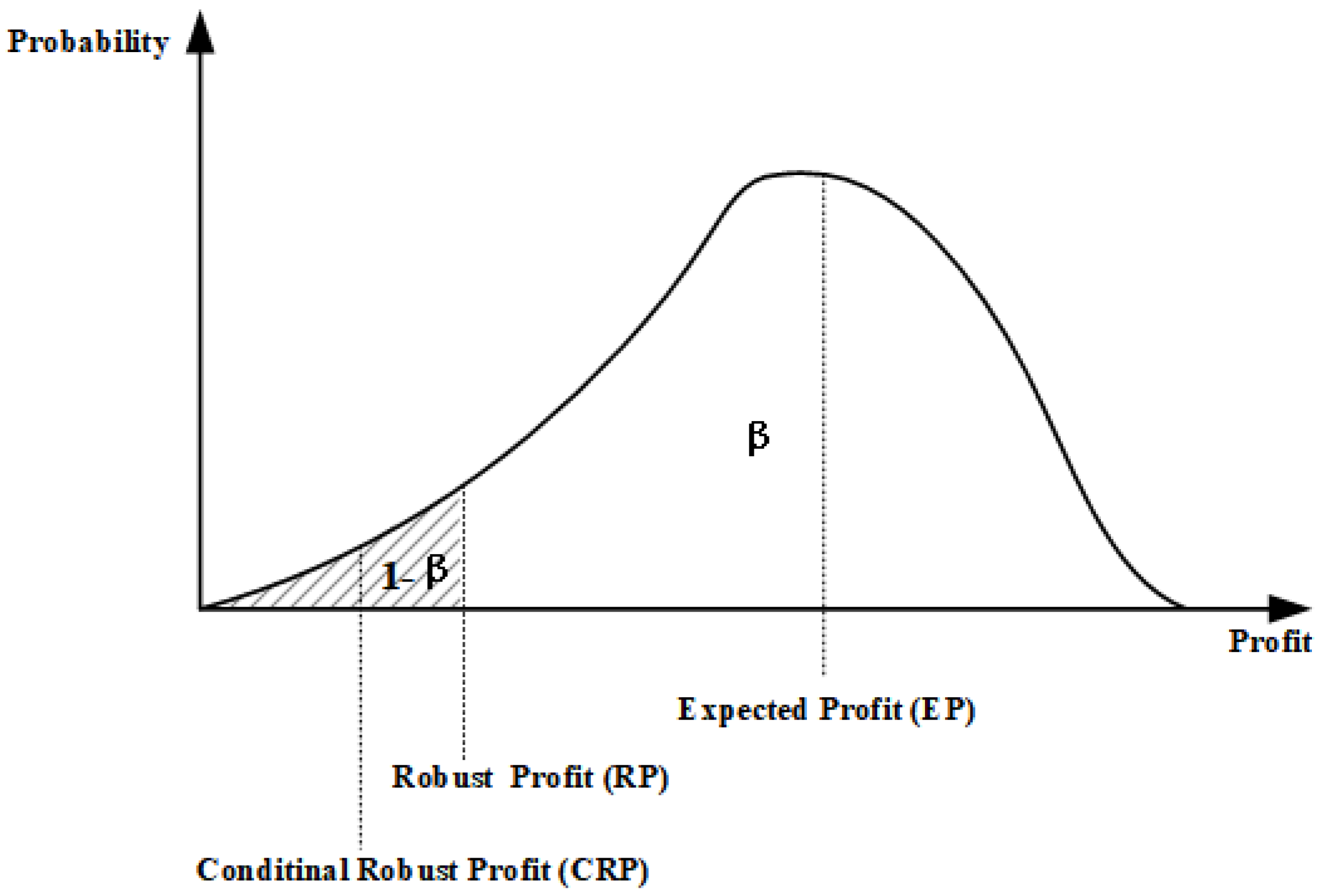
As discussed in [12], the VaR provides the estimation on the monetary loss a decision maker could suffer due to the fluctuations of uncertain parameters for a given probability of occurrence. The probability of occurrence, which can be also denoted as confidence level $\beta$, means that the probability that the loss exceeds $Va{R}_{\beta }$ is (1$-\beta$). Mathematically, $Va{R}_{\beta }$ is the difference between the expected profit and the lower 100(1$-\beta$) percentile of the profit distribution. As an alternative measure of risk to the VaR, the CVaR is defined as the average loss when the loss exceeds $Va{R}_{\beta }$. Mathematically, $CVa{R}_{\beta }$ is the difference between the expected profit and the average value of the 100(1$-\beta$)% of the lowest profit values. Based on the VaR and CVaR, the concepts of the RP and CRP [39] will be introduced in this section.

Let $\pi (X,\lambda )$ denote the profit function of a retailer where X represents the decision variables and $\lambda$ is the random parameter. In this paper, X denotes the volumes of electricity purchased from different options and the SL incentive price offered to the customers, $\lambda$ represents the DA market price. Let $p\left(\lambda \right)$ be the probability density distribution of the random parameter $\lambda$. The probability of the profit not falling below a threshold $\alpha$ is then given by

$$\psi (X,\alpha )=\underset{\pi (X,\lambda )\ge \alpha }{\int }p\left(\lambda \right)d\lambda$$

(1)

For a given confidence level $\beta \in (0,1)$, the RP under confidence level $\beta$ is given by Equation (2).

$$\begin{array}{c}\hfill R{P}_{\beta }\left(X\right)=max\{\alpha \in R:\psi (X,\alpha )\ge \beta \}\end{array}$$

(2)

In (2), $R{P}_{\beta }\left(X\right)$ is the RP of the retailer which comes out as the right endpoint of the nonempty interval consisting of the values of $\alpha$ such that $\psi (X,\alpha )=\beta$ with different X selected. The corresponding $Va{R}_{\beta }\left(X\right)$ would be the expected profit (EP) minus the $R{P}_{\beta }\left(X\right)$ given by (2) [12]. It is evident that $R{P}_{\beta }\left(X\right)$ merely provides the highest bound for profit in the tail of the profit distribution and has insufficient measurement of the tail profit. To overcome the shortage of the RP, the CRP is introduced in Equation (3):

$$\begin{array}{c}\hfill CR{P}_{\beta }\left(X\right)=\frac{1}{1-\beta }\underset{\pi (X,\lambda )\le R{P}_{\beta }\left(X\right)}{\int }\pi (X,\lambda )·p\left(\lambda \right)d\lambda \end{array}$$

(3)

$CR{P}_{\beta }\left(X\right)$ is the conditional expectation of the profit $\pi (X,\lambda )$ associated with X when the profit is not greater than $R{P}_{\beta }\left(X\right)$. The graphical representation of RP and CRP can be seen in Figure 1. And as stated in [39], the $CR{P}_{\beta }\left(X\right)$ given by (3) can also be described as EP minus the $CVa{R}_{\beta }\left(X\right)$. Therefore, the problem of maximizing $CR{P}_{\beta }\left(X\right)$ is equivalent to a multi-objective optimization problem in which equal weights are given to maximizing EP and minimizing $CVa{R}_{\beta }\left(X\right)$. Maximizing (3) with different $\beta$ can be considered as a trade-off between risk and profit. The retailer’s risk aversion level can be easily controlled by setting different values of the confidence level parameter. With increasing $\beta$, the retailer will become more risk-averse and seek a less risky strategy.

It should be noted that $R{P}_{\beta }\left(X\right)$ is an endogenous variable in Equation (3), which brings great difficulties to calculate $CR{P}_{\beta }\left(X\right)$ directly using Equation (3). Ref. [18] shows that $CR{P}_{\beta }\left(X\right)$ can be obtained by solving

$$\begin{array}{c}\hfill CR{P}_{\beta }\left(X\right)=max{G}_{\beta }(X,\alpha )\end{array}$$

(4)

where

$$\begin{array}{c}\hfill G_{\beta }(X,\alpha )=\alpha +\frac{1}{1-\beta }\int {[\pi (X,\lambda )-\alpha ]}^{-}·\left(\lambda \right)d\lambda \end{array}$$

(5)

and ${[\pi (X,\lambda )-\alpha ]}^{-}=min\{\pi (X,\lambda )-\alpha ,0\}$. The integral calculation in Equation (5) is complicated and difficult to solve, to simplify the optimization problem in (4), $G_{\beta }(X,\alpha )$ can be approximated by employing random sampling method to obtain a large number of scenarios of the DA market price according to the probability density distribution $p\left(\lambda \right)$. Assume that there are S scenarios which are denoted by ${\lambda }_{DA}^1,{\lambda }_{DA}^2,\dots ,{\lambda }_{DA}^S$, with the occurrence probability: $Pr\left({\lambda }_s\right)={\rho }_s$, $s=1,2,\dots ,S$ and

$$\begin{array}{c}\hfill \sum _{s=1}^S{\rho }_s=1\end{array}$$

(6)

then the retailer’s profit function in scenario s is denoted by $\pi (X,{\lambda }_{DA}^s)$ and the corresponding approximation to $G_{\beta }(X,\alpha )$ is

$$\begin{array}{c}\hfill {\tilde{G}}_{\beta }(X,\alpha )=\alpha +\frac{1}{1-\beta }\sum _{s=1}^S{\rho }_s·{[\pi (X,{\lambda }_{DA}^s)-\alpha ]}^{-}\end{array}$$

(7)

and the $CR{P}_{\beta }\left(X\right)$ can be calculated as

$$\begin{array}{c}\hfill CR{P}_{\beta }\left(X\right)=max{\tilde{G}}_{\beta }(X,\alpha )\end{array}$$

(8)

3. CRP-Based Bi-Level Decision-Making Model

3.1. Assumption

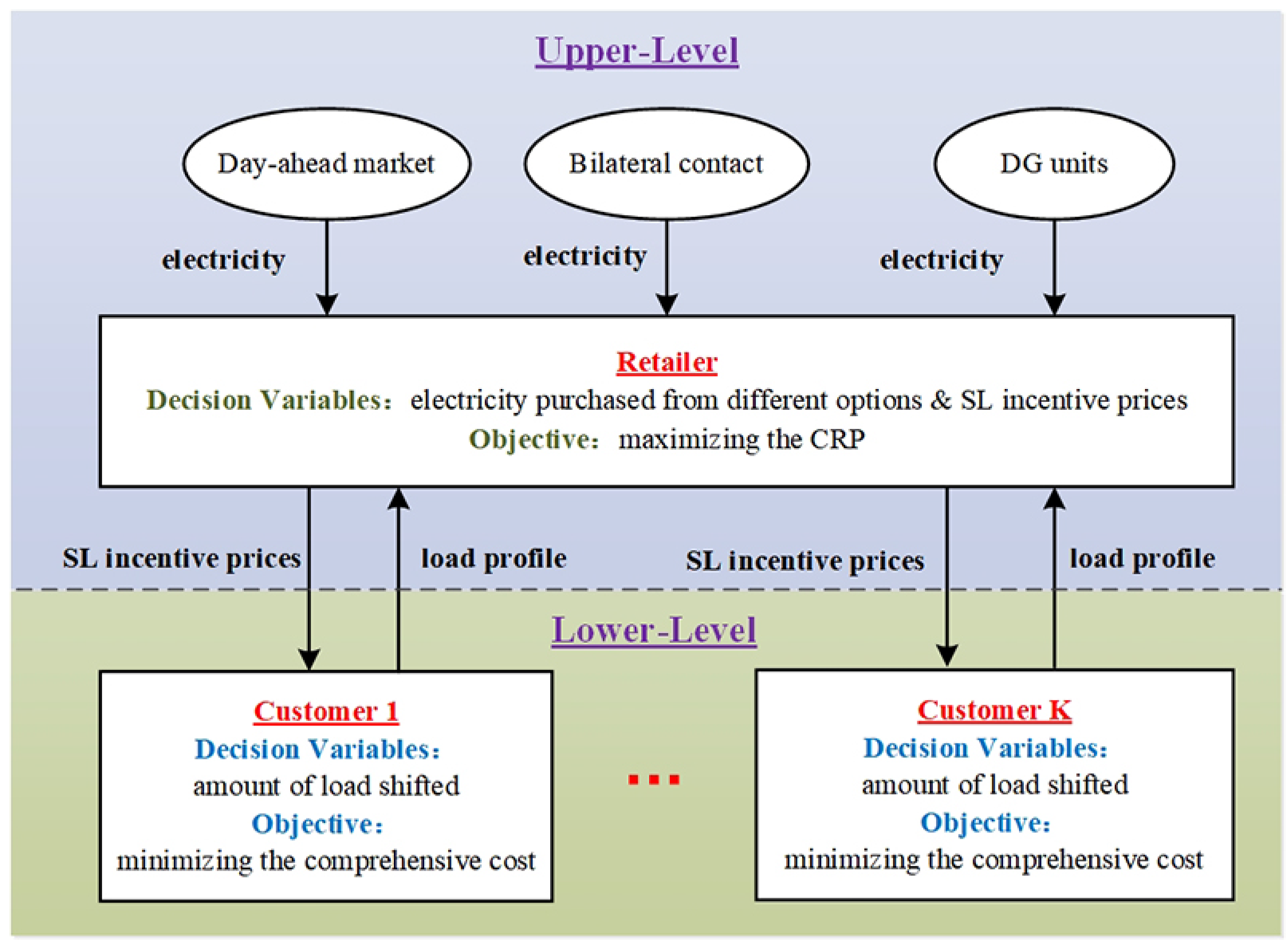
A risk-averse retailer acquires electricity from the DA wholesale market, bilateral contracts and self-owned DG units. Assume that the retailer behaves as a price-taker so that its electricity procurement strategy does not influence the purchased prices. In order to make full use of customers’ SL capability, the retailer not only pays incentive fees for customers’ load reduction during peak periods, but also has the motivation to provide incentive payments for the customers’ load increase during valley periods. Considering the uncertainty of the DA market prices, a CRP-based bi-level decision-making framework for the retailer’s energy procurement and SL incentive strategies are proposed in this paper. The framework of the bi-level model is shown in Figure 2. In the upper problem, the retailer specifies the volume of electricity acquired from each option and SL incentive prices offered to customers in order to maximize its CRP under confidence level $\beta$. In the lower problem, each customer shifts its load according to the incentive prices offered to minimize the comprehensive cost including the discomfort cost of electricity consumption.

3.2. Upper-Level Problem for Retailer’s CRP Maximization

In the upper-level problem, the retailer’s objective is to maximize its CRP under certain confidence level during T time periods. To cope with the uncertainty of the DA market prices, S scenarios of the DA market prices can be generated by a random sampling method based on the joint distribution function of the DA market prices. The scenarios are denoted by ${\lambda }_{DA}^s=[{\lambda }_{1,s}^{DA},{\lambda }_{2,s}^{DA},\dots ,{\lambda }_{T,s}^{DA}],s=1,2,\dots ,S$. ${\lambda }_{DA}^s$ is the set of the DA market prices during all time periods in scenario s, ${\lambda }_{t,s}^{DA}$ is the DA market price in time period t and scenario s. Let N and M denote the numbers of the bilateral contracts and the retailer’s self-owned DG units, respectively. There are K customers purchasing electricity from the retailer. Then the objective function of the retailer can be obtained as follows:

$$\begin{array}{c}max{\tilde{G}}_{\beta }(X,\alpha )=max\{\alpha +\frac{1}{1-\beta }\sum _{s=1}^S{\rho }_s·{[\pi (X,{\lambda }_{DA}^s)-\alpha ]}^{-}\}\end{array}$$

(9)

$$\begin{array}{c}\pi (X,{\lambda }_{DA}^s)=\sum _{t=1}^T\sum _{k=1}^K{\lambda }^{sell}·P_{k,t}^{real}-C_{DA}^s-C_{BC}-C_{DG}-C_{SL}\end{array}$$

(10)

$$\begin{array}{c}{C}_{DA}^s=\sum _{t=1}^T{\lambda }_{t,s}^{DA}·P_t^{DA}\end{array}$$

(11)

$$\begin{array}{c}{C}_{BC}=\sum _{t=1}^T\sum _{n=1}^N{\lambda }_{n,t}^{BC}·P_{n,t}^{BC}\end{array}$$

(12)

$$\begin{array}{c}{C}_{DG}=\sum _{t=1}^T\sum _{m=1}^M[a_m·{\left(P_{m,t}^{DG}\right)}^2+b_m·P_{m,t}^{DG}+c_m^{SU}·v_{m,t}+c_m^{SD}·w_{m,t}]\end{array}$$

(13)

$$\begin{array}{c}{C}_{SL}=\sum _{t\in T_{peak}}\sum _{k=1}^K{\lambda }_{k,t}^{SL}·(P_{k,t}^D-P_{k,t}^{real})+\sum _{t\in T_{valley}}\sum _{k=1}^K{\lambda }_{k,t}^{SL}·(P_{k,t}^{real}-P_{k,t}^D)\end{array}$$

(14)

In the objective function (9), the retailer aims to maximize its CRP under confidence level $\beta$. The retailer’s profit in scenario s is listed in Equation (10). The first term in Equation (10) denotes the revenue of the retailer where $p_{k,t}^{real}$ is the actual electricity demand of customer k in time period t and ${\lambda }^{sell}$ is the predetermined fixed selling price of the retailer. The terms $C_{DA}^s$, $C_{BC}$, $C_{DG}$ and $C_{SL}$ represent the costs of electricity purchasing in the DA wholesale market, bilateral contracts, DG units and the payments for customers’ load shifting, respectively. Equation (11) shows the total cost of electricity purchasing in the DA markets in scenario s. Equation (12) shows the total cost of electricity purchasing from bilateral contracts. Equation (13) shows the total cost of the DG units including quadratic generation cost, startup cost and shutdown cost. The payments for customers’ load shifting is expressed in Equation (14). The retailer offers incentive payments to motivate customers to shift their electricity consumptions from peak periods to valley periods as the deviation of actual demand from the desired demand will cause discomfort to customers. ${\lambda }_{k,t}^{SL}$ is the SL incentive price paid for per unit load of customer k deviated from his baseline load $P_{k,t}^D$ in time period t.

In the upper problem, the following constraints should be considered:

$$\begin{array}{c}{p}_{n,min}^{BC}·s_{n,t}\le P_{n,t}^{BC}\le p_{n,max}^{BC}·s_{n,t}\end{array}$$

(15)

$$\begin{array}{c}{p}_{m,min}^{DG}·u_{m,t}\le P_{m,t}^{DG}\le p_{m,max}^{DG}·u_{m,t}\end{array}$$

(16)

$$\begin{array}{c}{v}_{m,t}-w_{m,t}=u_{m,t}-u_{m.t-1}\end{array}$$

(17)

$$\begin{array}{c}\sum _{t^{\prime }=t-U{T}_m+1}^t{v}_{m,t^{\prime }}\le u_{m,t},\forall m,t\in U{T}_m,\dots ,24\end{array}$$

(18)

$$\begin{array}{c}\sum _{t^{\prime }=t-D{T}_m+1}^t{w}_{m,t^{\prime }}\le 1-u_{m,t},\forall m,t\in D{T}_m,\dots ,24\end{array}$$

(19)

$$\begin{array}{c}{P}_{m,t}^{DG}-P_{m,t-1}^{DG}\le R_m^{Up}·u_{m,t}\end{array}$$

(20)

$$\begin{array}{c}{P}_{m,t-1}^{DG}-P_{m,t}^{DG}\le R_m^{Down}·u_{m,t-1}\end{array}$$

(21)

$$\begin{array}{c}{P}_t^{DA}+\sum _{n=1}^N{P}_{n,t}^{BC}+\sum _{m=1}^M{P}_{m,t}^{DG}=\sum _{k=1}^K{P}_{k,t}^{real}\end{array}$$

(22)

The minimum and maximum volumes of electricity purchased from contract n in time period t are shown in constraint (15). The minimum and maximum outputs of the DG units are presented in constraint (16) and DG units’ startup and shutdown status are represented by Equation (17). Constraints (18) and (19) describe the minimum up/down time of DG units. Finally, the ramp up/down rate limits are expressed in constraints (20) and (21). The power balance constraint for the retailer in time period t is presented in Equation (22).

For calculation convenience, auxiliary variables $z_s(s=1,2,\dots ,S)$ are introduced to replace the term ${[\pi (X,{\lambda }_{DA}^s)-\alpha ]}^{-}$ in objective function (9). The above model then can be transformed into the model shown in (23)–(26) where the retailer’s decision variables are expressed by $X=[P_t^{DA},P_{n,t}^{BC},P_{m,t}^{DG},{\lambda }_{k,t}^{SL}]$.

$$\begin{array}{c}\hfill max[\alpha +\frac{1}{1-\beta }\sum _{s=1}^S{\rho }_s·z_s]\end{array}$$

(23)

Subject to:

$$\begin{array}{c}{z}_s\le \pi (X,{\lambda }_{DA}^s)-\alpha \end{array}$$

(24)

$$\begin{array}{c}{z}_s\le 0\end{array}$$

(25)

$$\begin{array}{c}\mathrm{Constraints} \left(10\right)-\left(22\right)\end{array}$$

(26)

3.3. Lower-Level Problems for Customers’ Cost Minimization

The comprehensive cost function $C_k$ of customer k is shown in objective function (27) which includes the cost of purchasing electricity from the retailer, discomfort cost caused by load shifting and the SL payments received from the retailer. Each customer aims to minimize his comprehensive cost $C_k$ after load shifting. The decision variable of customer k is the actual load demand $P_{k,t}^{real}$. In the lower-level problem, each customer’s decision-making model can be formulated as follows:

$$\begin{array}{c}\hfill min{C}_k=min[\sum _{t=1}^T{z}_{k,t}\left(P_{k,t}^{real}\right)+\sum _{t=1}^T{\lambda }^{sell}{P}_{k,t}^{real}-C_{SL}]\end{array}$$

(27)

Subject to:

$$\begin{array}{c}{z}_{k,t}(P_{k,t}^{real})=d_k·{(P_{k,t}^D-P_{k,t}^{real})}^2\end{array}$$

(28)

$$\begin{array}{c}(1-\epsilon )·P_{k,t}^D\le P_{k,t}^{real}\le P_{k,t}^D\hspace{1em}\hspace{1em}t\in T_{peak}\end{array}$$

(29)

$$\begin{array}{c}{P}_{k,t}^D\le P_{k,t}^{real}\le (1+\epsilon )·P_{k,t}^D\hspace{1em}\hspace{1em}t\in T_{valley}\end{array}$$

(30)

$$\begin{array}{c}\sum _{t=1}^T{P}_{k,t}^{real}=\sum _{t=1}^T{P}_{k,t}^D\end{array}$$

(31)

$z_{k,t}(P_{k,t}^{real})$ in Equation (28) denotes customer k’s discomfort cost function where $d_k$ is the positive parameter which transforms customer k’s discomfort caused by rescheduling his electricity consumption into cost. Shifting the same amount of electricity will bring larger discomfort cost to the customer with a larger $d_k$, so customer with larger $d_k$ is less willing to shift his load. The upper and lower limits of actual demand of customer k in peak periods and valley periods are shown in constraints (29) and (30) respectively. Equation (31) indicates that after load shifting, the total load demand of the customer during T periods cannot be changed.

3.4. Mathematical Reformulation of the Bi-Level Model

Because the lower-level problems are convex when the incentive prices are fixed, their Karush-Kuhn-Tucker (KKT) conditions are both necessary and sufficient for optimality. Therefore, the bi-level model can be transformed into a non-linear complementarity model by replacing the lower-level problems with their KKT conditions. The KKT conditions of the lower-level model are derived as (32)–(34) where ${\mu }_{k,nt},{\gamma }_k$ are Lagrange multipliers introduced during the reformulation.

$$\begin{array}{c}\left\{\begin{array}{c}\hfill 2d_k·(P_{k,t}^{real}-P_{k,t}^D)+{\lambda }^{sell}+{\lambda }_{k,t}^{SL}-{\mu }_{k,1t}+{\mu }_{k,2t}+{\gamma }_k=0,t\in T_{peak}\\ \hfill 2d_k·(P_{k,t}^{real}-P_{k,t}^D)+{\lambda }^{sell}-{\lambda }_{k,t}^{SL}-{\mu }_{k,3t}+{\mu }_{k,4t}+{\gamma }_k=0,t\in T_{valley}\end{array}\right.\end{array}$$

(32)

$$\begin{array}{c}\left\{\begin{array}{c}\hfill {\mu }_{k,1t}·(P_{k,t}^{real}-(1-\epsilon )P_{k,t}^D)=0\\ \hfill {\mu }_{k,2t}·(P_{k,t}^D-P_{k,t}^{real})=0\\ \hfill {\mu }_{k,3t}·(P_{k,t}^{real}-P_{k,t}^D)=0\\ \hfill {\mu }_{k,4t}·((1+\epsilon )P_{k,t}^D-P_{k,t}^{real})=0\\ \hfill {\mu }_{k,1t},{\mu }_{k,2t},{\mu }_{k,3t},{\mu }_{k,4t}\ge 0\end{array}\right.\end{array}$$

(33)

$$\begin{array}{c}\sum _{t=1}^T{P}_{k,t}^{real}-\sum _{t=1}^T{P}_{k,t}^D=0\end{array}$$

(34)

The bi-level model after reformulation can be expressed as follows:

$$\begin{array}{c}max[\alpha +\frac{1}{1-\beta }\sum _{s=1}^S{\rho }_s·z_s]\end{array}$$

(35)

$$\begin{array}{c}\mathrm{Subject} \mathrm{to} \left(24\right)-\left(26\right),\left(32\right)-\left(34\right)\end{array}$$

(36)

Since constraints in (33) are non-linear complementary constraints, the Fortuny-Amat McCarl linearization method in [40] is adopted to transform these constraints into linear constraints for calculation convenience. The model after reformulation is a mixed-integer non-linear programming (MINLP) problem that can be solved using SBB solver under GAMS optimization software.

4. Case Study

4.1. Data Assumption

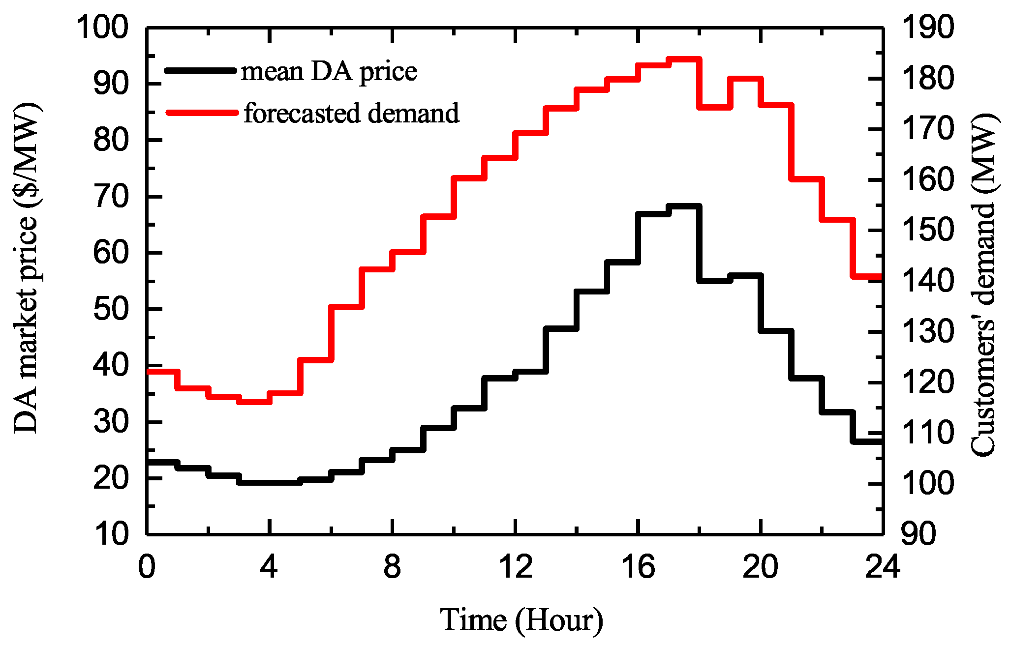
For the DA market price uncertainty modeling, we use the observed DA market prices ${\lambda }_t^{ave}$ of PJM market as mean values for the scenarios which is shown in Figure 3 [41]. Scenarios of the DA market prices are generated based on ${\lambda }_t^{ave}$ by simulating a multivariate Gaussian process with an exponentially decreasing covariance structure [42], i.e., the (i, j)-th element of the covariance matrix is given by

$$\begin{array}{c}C(i,j)={\sigma }_i·{\sigma }_j·e^{-|i-j|/\tau }\end{array}$$

(37)

$$\begin{array}{c}{\sigma }_t=\kappa ·{\lambda }_t^{ave}\end{array}$$

(38)

where ${\sigma }_t$ is the standard deviation in time period t which is proportional to the observed mean price. The parameter $\tau$ sets the exponential decay of correlation with respect to the time lag. As the $\tau$ increases, the decay of correlation with respect to the time lag slows down. In (38), parameter $\kappa$ is used to denote the degree of uncertainty of the DA market prices, the greater the parameter $\kappa$, the larger the DA market price uncertainty. In this case study, $\kappa$ and $\tau$ is set as 0.1 and 5, respectively. 1000 scenarios of the DA market prices are generated by Monte Carlo method, and the occurrence probability of each scenario is the same.

The customers are divided into two categories, i.e., industrial customers and commercial customers, and each category of customers has the same baseline load profile. The aggregated base demand of all customers is also shown in Figure 3. Parameter $\epsilon$ of all customers is set as 10%. It is considered that load-shifting has less negative impact on the industrial customers, as such the discomfort cost coefficients $d_k$ for the industrial and commercial customers are set as 0.8 and 1, respectively. The parameters of bilateral contracts and DG units are shown in

Table 1. Parameters of bilateral contracts.

Contract No.	Min (MWh)	Max (MWh)	Price ($/MWh)
1	6	20	45
2	5	20	25
3	4	25	30
4	5	20	42

and

Table 2. Parameters of distributed generation (DG) units.

	DG Unit 1	DG Unit 2
Min.Output (MWh)	0.5	0.5
Max.Output (MWh)	25	25
$a_m$ ($/${\left(\mathrm{MW}\right)}^2$h)	0.015	0.02
$b_m$ ($/MWh)	38	45
Ramp Up Rate (MWh)	4	3
Ramp Down Rate (MWh)	4	3
Startup Cost ($)	50	40
Shutdown Cost ($)	100	200

respectively. The customers are encouraged to reduce load demand during peak periods, i.e., hours 11–22, and shift the reduced load to valley periods, i.e., hours 1–10 and hours 23–24.

4.2. Simulation Results

4.2.1. Strategies under Different Confidence Levels

Table 3. RP, CRP, average profit and standard deviation under different confidence levels.

	$\mathit{\beta }=0.89$	$\mathit{\beta }=0.91$	$\mathit{\beta }=0.93$	$\mathit{\beta }=0.95$	$\mathit{\beta }=0.97$	$\mathit{\beta }=0.99$
RP($)	168,939.1	168,384.7	167,862.4	167,429.8	166,726.8	165,665.1
CRP($)	167,367.8	167,085.1	166,784.6	166,434.3	165,970.4	165,288.5
Average profit($)	173,347.8	173,334.4	173,284.0	173,278.9	173,188.6	172,842.87
Standard deviation($)	111.77	111.52	110.66	110.59	109.03	104.23

shows the retailer’s optimal RP, CRP, average profit and standard deviation of its profit distribution under different confidence level $\beta$. It is shown that the retailer’s RP and CRP decrease when its confidence level $\beta$ increases. A retailer with higher confidence level aims to reduce the occurrence probability that its profit falls below the RP, so a smaller RP will be obtained by the retailer and the CRP also decreases at the same time. For instance, the RP obtained by the retailer is USD 167,429.8 when $\beta =0.95$, which means that the probability that the retailer’s profit is lower than USD 167,429.8 is 5%; the CRP equals to USD 166,434.3, so the expected profit of the retailer when its profit falls below the RP is USD 166,434.3. It can be seen from Table 3 that the retailer will obtain a smaller average profit with a smaller standard deviation of profit as the confidence level increases. In other word, when the retailer chooses a more conservative strategy, the risk exposed to the retailer decreases, but at the expense of its average profit. The above results demonstrate that by maximizing the CRP under different confidence levels, the retailer can achieve a reasonable tradeoff between reward and risk.

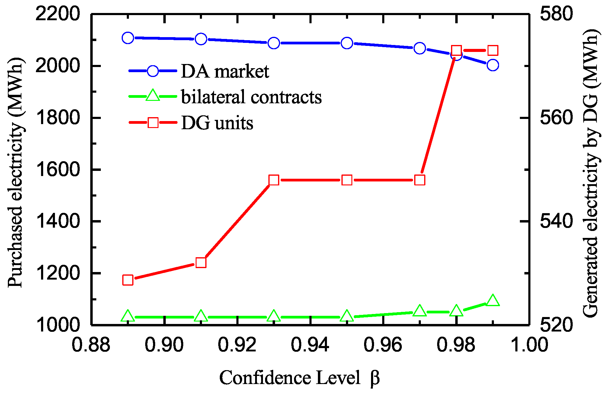
Figure 4 shows the volumes of electricity procured by the retailer from different options during all time periods under different confidence levels. As shown in Figure 4, with increasing $\beta$, the volume of electricity procured from the DA market decreases while the volumes of electricity purchased from bilateral contracts and DG units increase. The volatility of the DA market prices makes it riskier to purchase electricity from the DA market than from other options. As such, when the retailer is more risk-averse, it will reduce the electricity purchased in the DA market.

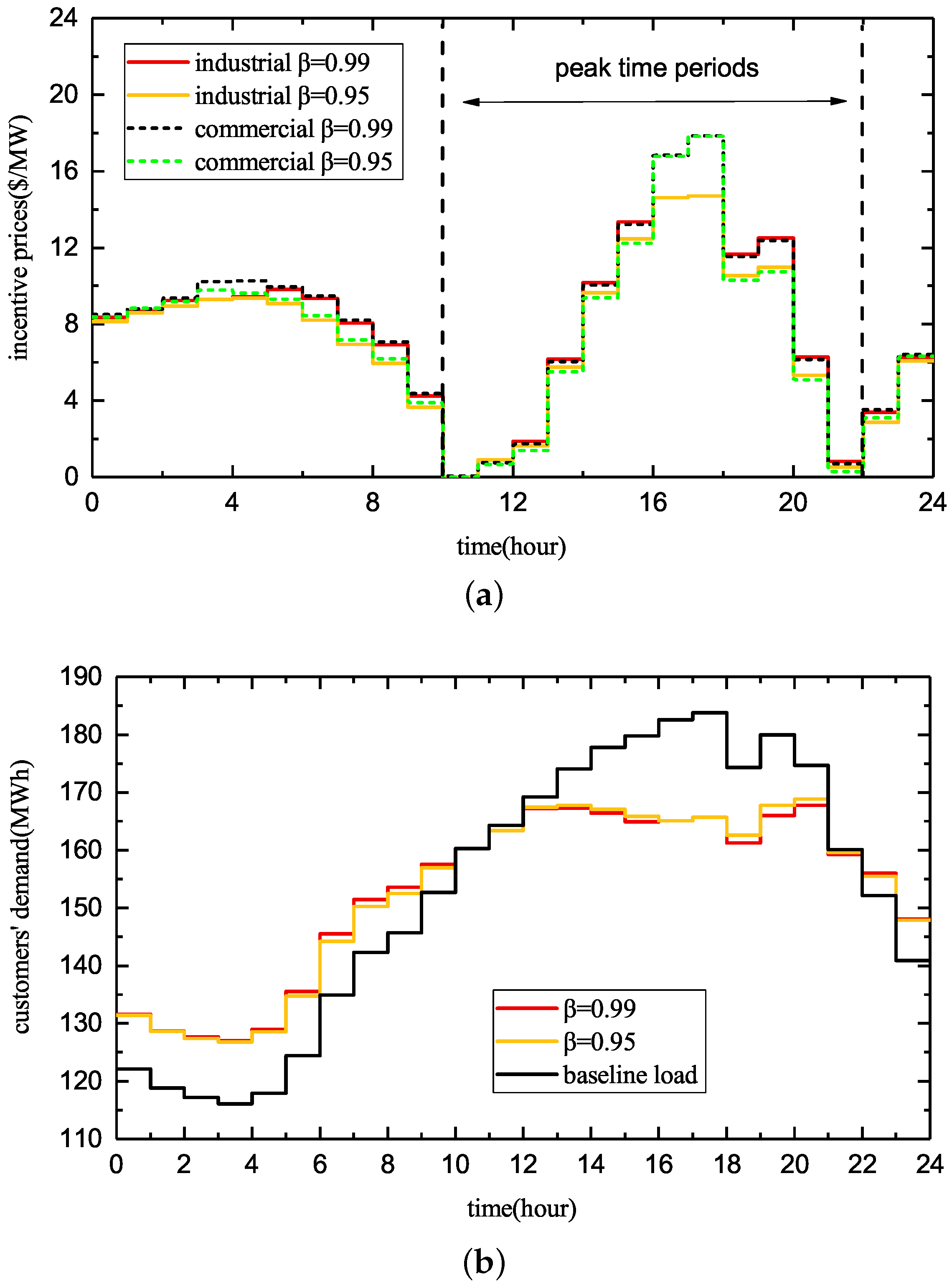
The retailer’s SL incentive prices and its customers’ actual load demand under different confidence levels are illustrated in Figure 5. For a given $\beta$, during the peak periods, the retailer offers higher incentive prices for the customers in order to encourage customers to reduce more load in the time period with higher mean DA market price. Contrarily, during the valley periods, the retailer offers higher SL incentive prices to encourage customers to shift more load to the time period with lower mean DA market price, thus decreases the electricity procurement cost.

It can be also seen in Figure 5 that with increasing confidence level, the SL incentive prices offered to customers increase during some time periods so that the customers shift more load from peak periods to valley periods. It can be noted from Equations (37) and (38) that a higher mean market price will lead to larger fluctuation of the market price which brings more risk to the retailer. When the customers shift more load from peak periods to valley periods, the risk caused by the fluctuation of the DA market prices decreases. The total SL incentive payments of the retailer and the total amount of customers’ shifted load under different confidence level $\beta$ are presented in

Table 4. SL incentive payments of the retailer and the amount of customers’ shifted load under different confidence levels.

	$\mathit{\beta }=0.91$	$\mathit{\beta }=0.93$	$\mathit{\beta }=0.95$	$\mathit{\beta }=0.97$	$\mathit{\beta }=0.99$
SL incentive payments ($)	1891.43	1920.54	1963.46	1993.38	2195.44
Amount of load shifted (MW)	97.61	98.51	99.56	100.47	104.23

. The results demonstrate that with increasing the retailer’s risk-aversion level, more incentive fees are paid to encourage customers to shift more load, thereby reducing the retailer’s risk.

4.2.2. Strategies for Different Uncertainty of Market Prices

The degree of uncertainty of the DA market prices is represented by the parameter $\kappa$ in (38). In this section, the confidence level $\beta$ is set as 0.97.

Table 5. RP, CRP, average profit and standard deviation under different $\kappa$.

	$\mathit{\kappa }=0.05$	$\mathit{\kappa }=0.075$	$\mathit{\kappa }=0.1$	$\mathit{\kappa }=0.125$	$\mathit{\kappa }=0.15$
RP ($)	169,916.0	168,453.9	166,726.8	164,976.2	163,016.5
CRP ($)	169,024.8	167,270.5	165,970.4	163,752.0	161,525.4
Average profit ($)	173,531.2	173,451.4	173,188.6	172,874.3	171,882.6
Standard deviation ($)	57.94	86.36	109.03	131.54	145.53

shows the retailer’s optimal RP, CRP, average profit and standard deviation of its profit distribution under different $\kappa$. The larger the DA market price uncertainty, the less profit the retailer may achieve and the more risk the retailer faces. It can also be seen from Table 5 that with increasing DA market price uncertainty, both the optimal RP and CRP decrease. The volumes of electricity procured by the retailer from different options during all time periods under different $\kappa$ are shown in Figure 6. With increasing $\kappa$, the volume of electricity purchased in the DA market decreases while the volumes of electricity procured from the bilateral contracts and self-owned DG units increase.

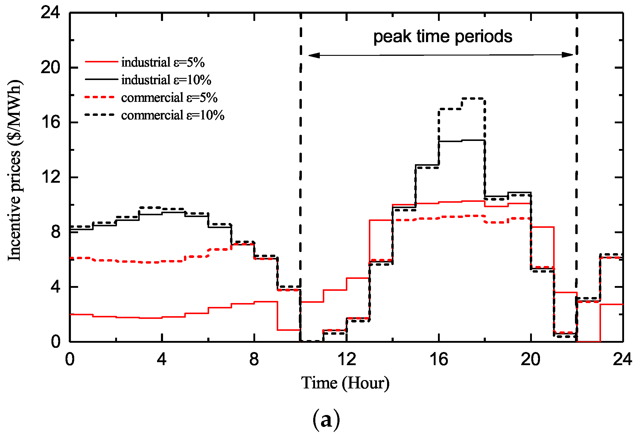
Figure 7 depicts the SL incentive prices of the retailer and customers’ actual load demand under different $\kappa$.

Table 6. SL incentive payments of the retailer and the amount of customers’shifted load under different $\kappa$.

	$\mathit{\kappa }=0.05$	$\mathit{\kappa }=0.075$	$\mathit{\kappa }=0.1$	$\mathit{\kappa }=0.125$	$\mathit{\kappa }=0.15$
SL incentive payments ($)	1829.23	1929.15	1993.38	2055.88	2119.29
Amount of load shifted (MW)	95.90	98.40	100.47	102.19	104.03

shows the SL incentive payments of the retailer and the amount of customers’ shifted load under different $\kappa$. With increasing $\kappa$, the SL incentive payments offered to the customers increase to encourage customers to shift more load from peak periods to valley periods. It can be seen from Figure 7 that during peak time periods, the SL incentive price increases more in the time period with higher mean DA market price; during valley time periods, the SL incentive price increases more in the time period with lower mean DA market price.

4.2.3. Strategies for Different Load-Shift Capability of Customers

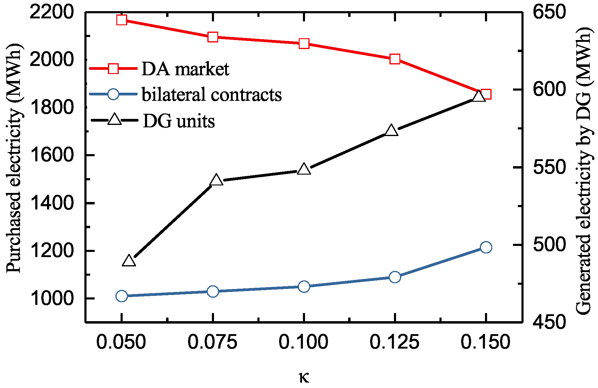
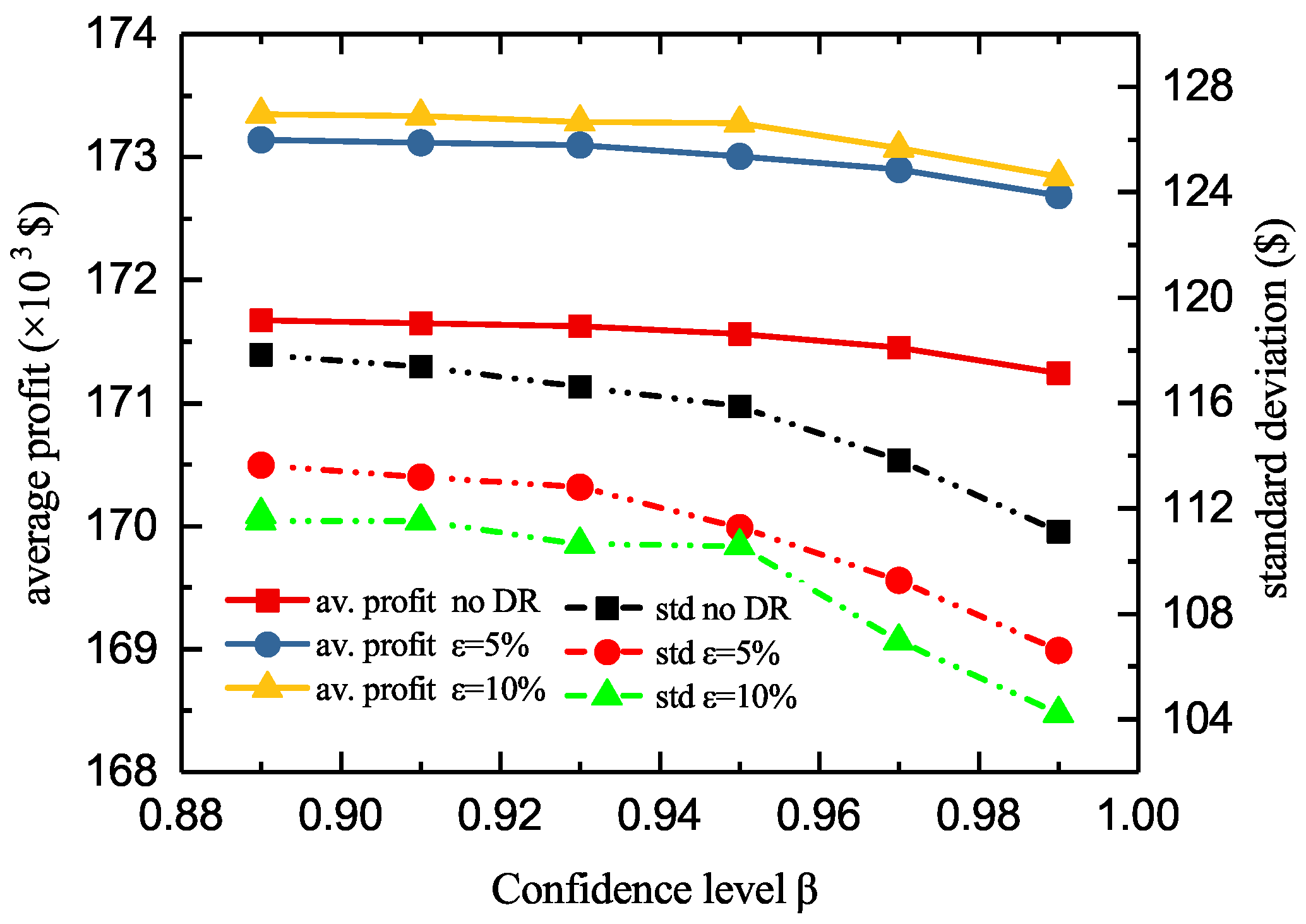
The customers’ load-shift capability is represented by the parameter $\epsilon$ and increases as the parameter $\epsilon$ increases. Figure 8 depicts the optimal CRP obtained by the retailer under different $\epsilon$. As shown in Figure 8, compared with the CRP obtained when customers’ SL capability is not considered, the retailer can obtain larger CRP under the same confidence level by deploying customers’ capability. And as the customers’ load-shift capability increases, the optimal CRP obtained also increases. Figure 9 depicts the the retailer’s average profit and the standard deviation of its profit distribution under different $\epsilon$. It is shown that with increasing customers’ load-shift capability, the retailer can obtain a larger average profit and a lower standard deviation under the same confidence level.

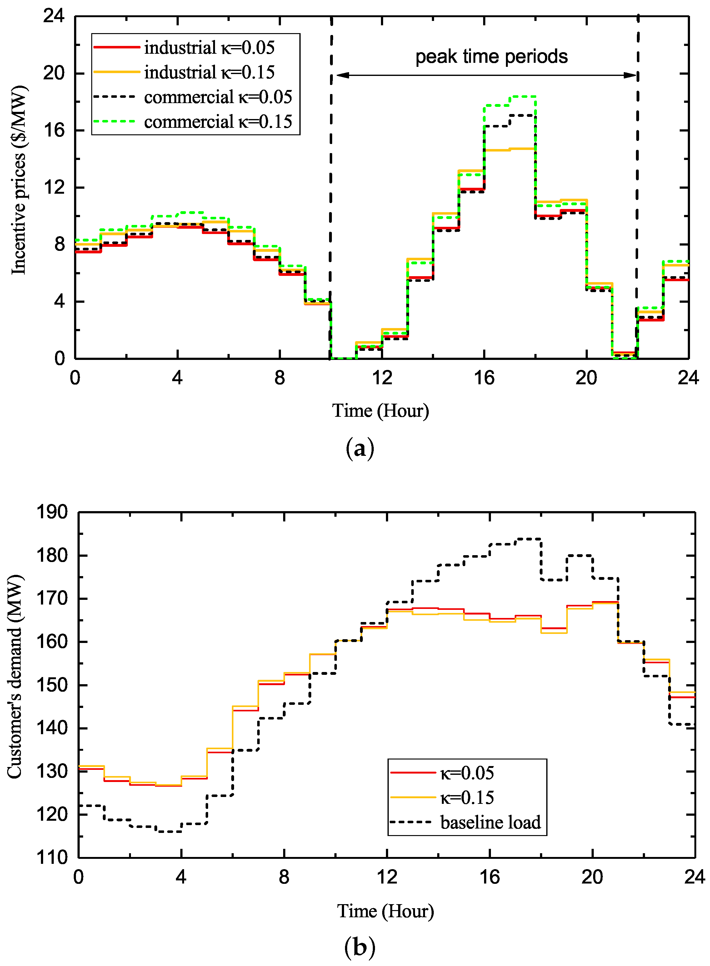
The retailer’s incentive prices and customers’ actual load demand under different $\epsilon$ when $\beta =0.97$ are shown in Figure 10. It can be found that with decreasing customers’ load-shift capability, the retailer will reduce the SL incentive prices offered to the customers and the total amount of load shifted by the customers decreases.

4.3. Discussions

The above results show that the retailer can achieve a trade-off between risk and reward by maximizing its CRP according to its risk aversion level. With increasing confidence level, the retailer becomes more risk-averse and specifies more conservative strategies to reduce the risk arising from the DA market price uncertainty. Specially, as the confidence level increases, the retailer will decrease the volume of electricity procured in the DA market and increases the SL incentive prices to encourage customers to shift more load from peak periods to valley periods. Besides, the larger the DA market price uncertainty, the more SL incentive payments the retailer will pay to encourage customers to shift more load. In addition, the retailer’s profit increases and the risk exposed to the retailer decreases as the load-shift capability of customers increases.

The main differences and advantages of our work compared to the related work are discussed as follows. In this paper, the retailer offers incentive payments for customers’ SL resources instead of the IL resources investigated in [30,31,32,34], and the case study results suggest that the SL is another important DR resource the retailer can deploy to improve its profit and reduce the risk caused by the market price uncertainty. In [31,32,33], the retailer’s incentive prices for DR resources are specified according to predetermined stepwise reward-based DR curves, however, in this paper the SL incentive prices are specified by solving a bi-level model which can better model the characteristics of customers, e.g., customers’ load-shift capability and customers’ willingness to participate in the DRP. In addition, in [33], a RO-based decision-making model is proposed to maximize retailer’s benefit in the worst case, however, over-conservative strategies may be obtained if the uncertainty set is not constructed properly. In [37], incentive strategies for the SL resources are studied but the market price uncertainty is neglected. In this paper, the CRP is introduced to help the risk-averse retailer achieve a trade-off between risk and reward by setting different confidence levels. Moreover, the approach proposed in this paper is also applicable for uncertainty models based on historical observations or scenarios and the analytical expression of the price distribution is not necessarily needed.

5. Conclusions

This paper investigates the problem of how to deploy customers’ SL for retailers’ risk management. The RP and CRP are used for a risk-averse retailer’s risk-reward trade-off analysis in its electricity procurement from various options. A CRP-based bi-level optimization model is proposed for the retailer to specify its electricity procurement strategy while taking customers’ incentive-based SL capability into consideration. In the upper problem, the retailer’s electricity procurement and SL incentive prices are specified to maximize its CRP under a given confidence level. The confidence level parameter can be used to examine the retailer’s energy procurement and SL incentive strategies under different risk-aversion levels. In the lower problem, customers shift load according to the SL incentive prices offered by the retailer so as to minimize their comprehensive costs including the discomfort cost of electricity consumption.

The validity of the model is verified by a case study. It is shown that the retailer can obtain larger profit and suffer less risk by deploying customers’ incentive-based SL capability. As such, it’s of great significance for retailers to design appropriate SL incentive program to make full use of customers’ SL resources. Furthermore, the model proposed in this paper is an effective risk-reward trade-off tool to help retailers with different risk aversion levels to specify electricity procurement and SL incentive strategies.

This paper only introduces the basic model of SL as the per-time-slot consumption limits or ramp constraints of SL are not considered, so a more complex and accurate model of SL should be introduced in future work. Besides, the uncertainty modeling of customers’ demand should also be taken into consideration in future research studies.

References

- Roncoroni, A.; Brik, R.I. Hedging size risk: Theory and application to the US gas market. Energy Econ. 2017, 64, 415–437. [Google Scholar] [CrossRef]
- Albadi, M.H.; El-Saadany, E.F. A summary of demand response in electricity markets. Electr. Power Syst. Res. 2008, 78, 1989–1996. [Google Scholar] [CrossRef]
- Huang, W.; Zhang, N.; Kang, C.; Li, M.; Huo, M. From demand response to integrated demand response: Review and prospect of research and application. Prot. Control Mod. Power Syst. 2019, 4, 12:1–12:13. [Google Scholar] [CrossRef] [Green Version]
- Hatami, A.; Seifi, H.; Sheikh-El-Eslami, M.K. A stochastic-based decision-making framework for an electricity retailer: Time-of-use pricing and electricity portfolio optimization. IEEE Trans. Power Syst. 2011, 26, 1808–1816. [Google Scholar] [CrossRef]
- Ma, T.; Wu, J.; Hao, L.; Yan, H.; Li, D. A real-time pricing scheme for energy management in integrated energy systems: A Stackelberg game approach. Energies 2018, 11, 2858. [Google Scholar] [CrossRef] [Green Version]
- Nojavan, S.; Mohammadi-Ivatloo, B.; Zare, K. Optimal bidding strategy of electricity retailers using robust optimisation approach considering time-of-use rate demand response programs under market price uncertainties. IET Gener. Transm. Distrib. 2015, 9, 328–338. [Google Scholar] [CrossRef]
- Attoh-Okine, N.O.; Ayyub, B.M. Applied Research in Uncertainty Modeling and Analysis; Springer: New York, NY, USA, 2005; ISBN 978-0-387-23535-6. [Google Scholar]
- Carvalho, P.M.S.; Ferreira, L.A.F.M.; Lobo, F.G.; Barruncho, L.M.F. Distribution network expansion planning under uncertainty: A hedging algorithm in an evolutionary approach. IEEE Trans. Power Deliv. 2000, 15, 412–416. [Google Scholar] [CrossRef]
- Kazerooni, A.K.; Mutale, J. Transmission network planning under security and environmental constraints. IEEE Trans. Power Syst. 2010, 25, 1169–1178. [Google Scholar] [CrossRef]
- Dueñas, P.; Reneses, J.; Barquin, J. Dealing with multi-factor uncertainty in electricity markets by combining Monte Carlo simulation with spatial interpolation techniques. IET Gener. Transm. Distrib. 2011, 5, 323–331. [Google Scholar] [CrossRef]
- Anton, S.G. The impact of enterprise risk management on firm value: Empirical evidence from romanian non-financial firms. Inz. Ekon. 2018, 29, 151–157. [Google Scholar] [CrossRef] [Green Version]
- Jabr, R.A. Generation self-scheduling with partial information on the probability distribution of prices. IET Gener. Transm. Distrib. 2010, 4, 138–149. [Google Scholar] [CrossRef]
- Boroumand, R.H.; Goutte, S.; Porcher, S.; Porcher, T. Hedging strategies in energy markets: The case of electricity retailers. Energy Econ. 2015, 51, 503–509. [Google Scholar] [CrossRef]
- Yang, J.; Zhao, J.; Wen, F.; Dong, Z.Y. A framework of customizing electricity retail prices. IEEE Trans. Power Syst. 2018, 33, 2415–2428. [Google Scholar] [CrossRef]
- Carrión, M.; Arroyo, J.M.; Conejo, A.J. A bilevel stochastic programming approach for retailer futures market trading. IEEE Trans. Power Syst. 2009, 24, 1446–1456. [Google Scholar] [CrossRef]
- Krokhmal, P.; Palmquist, J.; Uryasev, S. Portfolio optimization with conditional value-at-risk objective and constraints. J. Risk 2002, 4, 43–68. [Google Scholar] [CrossRef] [Green Version]
- Rockafellar, R.T.; Uryasev, S. Conditional value-at-risk for general loss distributions. J. Bank Financ. 2002, 26, 1443–1471. [Google Scholar] [CrossRef]
- Rockafellar, R.T.; Uryasev, S. Optimization of conditional value-at-risk. J. Risk 2000, 2, 21–42. [Google Scholar] [CrossRef] [Green Version]
- Ben-Tal, A.; Nemirovski, A. Robust optimization—Methodology and applications. Math. Program. 2002, 92, 453–480. [Google Scholar] [CrossRef]
- Nojavan, S.; Zare, K.; Mohammadi-Ivatloo, B. Robust bidding and offering strategies of electricity retailer under multi-tariff pricing. Energy Econ. 2017, 68, 359–372. [Google Scholar] [CrossRef]
- Liu, S.; Jian, J.; Wang, Y.; Liang, J. A robust optimization approach to wind farm diversification. Int. J. Electr. Power Energy Syst. 2013, 53, 409–415. [Google Scholar] [CrossRef]
- Bertsimas, D.; Sim, M. The price of robustness. Oper. Res. 2004, 52, 35–53. [Google Scholar] [CrossRef]
- Majidi, M.; Mohammadi-Ivatloo, B.; Soroudi, A. Application of information gap decision theory in practical energy problems: A comprehensive review. Appl. Energy 2019, 249, 157–165. [Google Scholar] [CrossRef] [Green Version]
- Nojavan, S.; Zare, K.; Mohammadi-Ivatloo, B. Risk-based framework for supplying electricity from renewable generation-owning retailers to price-sensitive customers using information gap decision theory. Int. J. Electr. Power Energy Syst. 2017, 93, 156–170. [Google Scholar] [CrossRef]
- Khojasteh, M.; Jadid, S. Decision-making framework for supplying electricity from distributed generation-owning retailers to price-sensitive customers. Util. Policy 2015, 37, 1–12. [Google Scholar] [CrossRef]
- Soroudi, A. Smart self-scheduling of Gencos with thermal and energy storage units under price uncertainty. Int. Trans. Electr. Energy Syst. 2014, 24, 1401–1418. [Google Scholar] [CrossRef] [Green Version]
- Hu, F.; Feng, X.; Cao, H. A short-term decision model for electricity retailers: Electricity procurement and time-of-use pricing. Energies 2018, 11, 3258. [Google Scholar] [CrossRef] [Green Version]
- Wei, W.; Liu, F.; Mei, S. Energy pricing and dispatch for smart grid retailers under demand response and market price uncertainty. IEEE Trans. Smart Grid 2015, 6, 1364–1374. [Google Scholar] [CrossRef]
- Ghazvini, M.A.F.; Soares, J.; Horta, N.; Neves, R.; Castro, R.; Vale, Z. A multi-objective model for scheduling of short-term incentive-based demand response programs offered by electricity retailers. Appl. Energy 2015, 151, 102–118. [Google Scholar] [CrossRef]
- Do Prado, J.C.; Qiao, W. A stochastic decision-making model for an electricity retailer with intermittent renewable energy and short-term demand response. IEEE Trans. Smart Grid 2019, 10, 2581–2592. [Google Scholar] [CrossRef]
- Mahmoudi, N.; Saha, T.K.; Eghbal, M. Developing a scenario-based demand response for short-term decisions of electricity retailers. In Proceedings of the 2013 IEEE Power & Energy Society General Meeting, Vancouver, BC, Canada, 21–25 July 2013. [Google Scholar]
- Nojavan, S.; Nourollahi, R.; Pashaei-Didani, H.; Zare, K. Uncertainty-based electricity procurement by retailer using robust optimization approach in the presence of demand response exchange. Int. J. Electr. Power Energy Syst. 2019, 105, 237–248. [Google Scholar] [CrossRef]
- Yu, X.; Lyu, X.; Luo, S.; Zhao, X.; Wang, X.; Yang, M. Power trading strategy and risk management for electricity retailers considering interruptible load. In Proceedings of the 2018 IEEE International Power Electronics and Application Conference and Exposition (PEAC), Shenzhen, China, 4–7 November 2018. [Google Scholar]
- Mohsenian-Rad, H. Optimal demand bidding for time-shiftable loads. IEEE Trans. Power Syst. 2015, 30, 939–951. [Google Scholar] [CrossRef]
- Ma, J.; Zhang, S.; Li, X.; Du, D. Integrating base-load cycling capacity margin in generation capacity planning of power systems with high share of renewables. Trans. Inst. Meas. Control 2020, 42, 31–41. [Google Scholar] [CrossRef]
- Feuerriegel, S.; Neumann, D. Measuring the financial impact of demand response for electricity retailers. Energy Policy 2014, 65, 359–368. [Google Scholar] [CrossRef] [Green Version]
- Sekizaki, S.; Nishizaki, I.; Hayashida, T. Electricity retail market model with flexible price settings and elastic price-based demand responses by consumers in distribution network. Int. J. Electr. Power Energy Syst. 2016, 81, 371–386. [Google Scholar] [CrossRef]
- Erkoc, M.; Al-Ahmadi, E.; Celik, N.; Saad, W. A game theoretic approach for load-shifting in the smart grid. In Proceedings of the 2015 IEEE International Conference on Smart Grid Communications (SmartGridComm), Miami, FL, USA, 2–5 November 2015; pp. 187–192. [Google Scholar]
- Jabr, R.A. Robust self-scheduling under price uncertainty using conditional value-at-risk. IEEE Trans. Power Syst. 2005, 20, 1852–1858. [Google Scholar] [CrossRef]
- Fortuny-Amat, J.; McCarl, B. A representation and economic interpretation of a two-level programming problem. J. Oper. Res. Soc. 1981, 32, 783–792. [Google Scholar] [CrossRef]
- PJM Markets and Operations. Available online: http://www.pjm.com/markets-and-operations/ (accessed on 13 July 2019).
- Zugno, M.; Morales, J.M.; Pinson, P.; Madsen, H. A bilevel model for electricity retailers’ participation in a demand response market environment. Energy Econ. 2013, 36, 182–197. [Google Scholar] [CrossRef]
Figure 1.
Graphical representation of robust profit (RP) and conditional robust profit (CRP).
Figure 2.
Framework of the bi-level model
Figure 3.
Observed mean day-ahead (DA) market prices and customers’ aggregated base demand.
Figure 4.
Volumes of electricity purchased under different confidence levels.
Figure 5.
(a) Shiftable load (SL) incentive prices under different confidence levels (b) Customers’ demand under different confidence levels.
Figure 6.
Volumes of electricity purchased under different .
Figure 7.
(a) SL incentive prices under different (b) Customers’ demand under different .
Figure 8.
CRP for different load-shift capability.
Figure 9.
Average profit and standard deviation of profit for different load-shift capability.
Figure 10.
(a) SL incentive prices for different load-shift capability (b) Customers’ demand for different load-shift capability.