Article

Impact of Long-Term Water Inflow Uncertainty on Wholesale Electricity Prices in Markets with High Shares of Renewable Energies and Storages

Institute of Energy Economics and Rational Energy Use (IER), University of Stuttgart, Heßbrühlstraße 49a, 70565 Stuttgart, Germany
*
Author to whom correspondence should be addressed.
Current address: Heßbrühlstraße 49a, 70565 Stuttgart, Germany.
Submission received: 28 February 2020 / Revised: 1 May 2020 / Accepted: 2 May 2020 / Published: 8 May 2020
(This article belongs to the Special Issue Uncertainties and Risk Management in Competitive Energy Markets)

Abstract

:
Renewable energy shares in electricity markets are increasing and therefore also require an increase in flexibility options. Conventional electricity price modelling with optimisation models in thermally dominated markets is not appropriate in markets with high shares of renewable energies and storages because price structures are not adequately represented. Previous research has already identified the impact of uncertainty in renewable energy feed-in on investment and dispatch decisions. However, we are not aware of any work that investigates the influence of uncertainties on price structures by means of optimisation models. Appropriate modelling of electricity price structures is important for investment and policy decisions. We have investigated the influence of uncertainty concerning water inflow by applying a second stage stochastic dual dynamic programming approach in a linear optimisation model using Norway as an example. We found that the influence of uncertainty concerning water inflow combined with high shares of storages has a strong impact on the electricity price structures. The identified structures are highly influenced by seasonal water inflow, electricity demand, wind, and export profiles. Additionally, they are reinforced by seasonal primary energy source prices and import prices. Incorporating uncertainties in linear optimisation models improves the price modelling and provides, to a large extent, an explanation for the seasonal patterns of Norwegian electricity market prices. The paper explains the basic pricing mechanisms in markets with high shares of storages and renewable energies which are subject to uncertainty. To identify these fundamental mechanisms, we focused on uncertainty regarding water inflow, but the basic results hold true for uncertainties regarding other renewable energies as well.

1. Introduction

Electricity markets today are increasingly moving towards systems based on renewable energies. This results in the additional need for flexibility options. If renewable energies should provide most of the power, seasonal storages or similar flexibility options become more relevant. For example, the expansion of flexibility options in Germany is, among other things, reflected by the construction of transmission capacities to Norway, to utilize existing storage capacities. As renewable energies depend upon uncertain factors like water inflow, wind or solar irradiation, long-term uncertainty regarding these factors will become more important.
As electricity markets are changing, it is likely that electricity market price structures will also change. Predicting electricity market prices is important for estimating investment decisions and retail prices as well as supporting policy decision regarding, e.g., subsidies. Hence, it is important to be able to at least roughly model electricity market prices in markets with high shares of renewable energies and storages. To date, most countries had a thermally dominated power plant park and the focus of price modelling was not on markets with high shares of renewable energies and storages.
In contrast, Norway is a country which already has a high share of renewable energies and storages. In addition, 96.3% of Norway’s electricity production comes from hydro power plants and 1.4% from wind power (2017) [1]. It has a storage capacity of 88 TWh, which means that 2 / 3 of the yearly Norwegian electricity demand can be stored (2017) [1]. The Norwegian electricity market is therefore well suited for testing price modelling methods in markets with a high share of renewable energies and storages.
There are several types of models to model prices, e.g., statistical models, optimisation models, simulation models or hybrids. Every type of model has its strengths and weaknesses, but we believe that getting prices right in optimisation models is especially important for forecasting long-term electricity prices. This has two main reasons. First, optimisation models are used in energy economics to calculate cost-optimal pathways towards a decarbonized electricity system or to analyse the impact of certain policies (e.g., CO 2 taxes, price zones, etc.). Subsequently, these pathways or policies are often analysed with regard to contribution margins of certain technologies and customer prices. Modelled electricity prices can be directly linked to a certain pathway or policy. Second, optimisation models are suited to investigate structural changes in the energy system, which is difficult for statistical models as they rely on historical data. Therefore, optimisation models can provide an insight on how electricity prices will develop under different conditions.
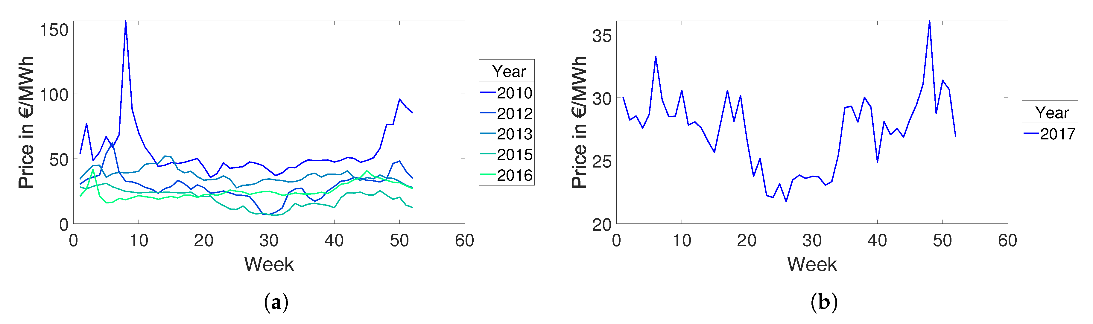
However, optimisation models should be able to capture the right trends and structure of electricity market prices. Under the assumption of an ideal market, in a thermally dominated power plant fleet, the marginal costs of production of the most expensive power plant are price-setting if the start-up and shut-down costs are neglected. With an increasing share of renewable energies, this would lead to a drop in prices for the majority of hours in the year. However, in markets with a high ratio of storage facilities, opportunity costs must also be taken into account and opportunity costs depend on expectations for the future. The average annual electricity market prices in Norway are about 36 €/MWh and clearly show seasonal structures (considered years: 2008–2017) [1]. These seasonal structures are not adequately captured by deterministic models. We believe that long-term uncertainty has an impact on the modelled price structure in markets with high shares of renewable energies and storages. Therefore, it is also becoming more relevant for countries like Germany.
There is some literature on electricity spot price modelling with optimisation models, e.g., [2,3,4,5]. In [2], both the day-ahead and the reserve market are modelled, while the other papers mentioned focus on the day ahead or intraday market. In [3,4,5], an attempt is made to better meet price structures, as the price curves modelled with optimisation models are often too flat. In [3], bidding mark-ups, e.g., start-up costs and risk premiums are added to the model. In [5], the factors for price formation that cannot be explained by a fundamental optimisation model are explained with the help of a regression model, where the “main differences can be attributed to (avoided) start up-costs, market states and trading behavior” [5]. The authors of [4] analyse the impact of too narrow margins in modelled electricity prices on storages. In their model, the authors allow bids under and over the marginal production costs. For modelling purposes, however, historical storage production is subtracted from demand as a fixed hydrograph. However, these papers focus more on short-term modelling than on seasonal price variations. Therefore, they do not examine the influence of uncertainty on intra-year price structures. Additionally, the above-mentioned papers do not focus on markets with high shares of renewable energies and storages.
The importance of modelling uncertainty of intermittent renewable energies in hydro-thermal power plant parks for flexibility investments as well as (hydro) power plant scheduling is shown by several authors (e.g., [6,7]). Research on and use of stochastic modelling in markets with high shares of renewable energies and storages is widespread (e.g., [8,9,10,11,12,13,14,15,16]). However, these papers do not deal with the influence of uncertainty on electricity market prices.
We found the following papers that examine the relationship between long-term uncertainty and electricity market prices. In [17], the authors name the most important factors for modelling Norwegian electricity market prices. One of them is uncertainty regarding water inflow. They examine the effects of aggregated hydro power and temperature-dependent demand on electricity prices in case studies. Although the authors include uncertainty regarding water inflow into their model with a stochastic dual programming (SDP) approach, they do not analyse the impact of modelling uncertain water inflow on electricity prices. The authors of [18] use a stochastic dual dynamic programming (SDDP) approach to address uncertainty. Their model is, among other things, used to model electricity market prices. However, they do not investigate the influence of modelling uncertainty on electricity prices. The authors of [19] use a model similar to the one used in [18]. Both models are based on the SDDP approach presented by [20]. In [19], the authors compare the SDP approach of [17] with two SDDP approaches regarding electricity price modelling. The first one uses a statistical model to generate water inflow scenarios for the optimisation as well as the simulation. We denote this model with SDDP-1. The second approach uses the statistical model for the optimisation, but for the simulation historical inflow series are used (SDDP-2). When comparing the SDP approach to the SDDP-1 approach, they found out that the prices modelled with the SDP model are more volatile and higher than in the compared model. In contrast to that, the modelled prices of the SDDP-2 model are higher and more volatile than those of the SDP model. The authors of [21] point out that those statistical models tend to underestimate the variance of the error term and thus underestimate extreme events. It is therefore likely that the SDDP-2 model has higher and more volatile prices than the SDDP-1 model for the following reason: The optimisation has not taken into account these more extreme water inflows, but the model still had to cope with them when the historic water inflow series realized in the simulation. The authors of [21] propose a two stage SDDP model where both the water inflow series for the optimisation and the simulation are historical. The main objective of the paper was to develop a model that can deal with uncertainty as well as possible. As prices with this approach are less volatile and lower than those of the SDDP-2 model in [19], the authors conclude that their model is better, as it can cope better with realistic water inflow series.
The literature review shows that modelling long-term uncertainty definitely has an impact on electricity prices in a market with a high share of renewable energies and storages. Different modelling approaches regarding uncertainty lead to different electricity prices. However, it is still open how uncertainty influences price structures within a year. Moreover, it is open which error occurs in not modelling uncertainty and thus it is not possible to deduce the importance of modelling uncertainty. Furthermore, if uncertainty affects electricity prices, there is a lack in understanding why it does affect electricity prices and which factors change the impact of uncertainty.
Our main findings are that uncertainty regarding water inflow combined with high shares of storages has a major influence on the structure of modelled electricity market prices. Water inflow, demand, and export profiles lead to a seasonal price structure when considering uncertainty of water inflow. Seasonal prices for primary energy sources and import intensify this effect. The higher the uncertainty of water inflow, the higher is the effect on the structure of electricity prices. Uncertainty has a significant influence in markets with a high share of renewable energies and storages because of two reasons. First, the inflow of water is afflicted with relatively high uncertainty. Second, the value of the energy in storages depends on the expected value of the future price scenarios. By modelling uncertainty, we recognise the seasonal price structures that exist in Norway. We conclude that the modelling of uncertainty concerning water inflow is an important factor for modelling prices with optimisation models in markets with high shares of storage. The principle price building mechanisms and effects shown in this paper also hold true for other uncertainties that have seasonal profiles like wind, sun or demand uncertainty. The impact of such other uncertainties depend on the height of uncertainty and in case of renewable energies on the shares in the system. As wind energy capacity is growing e.g., in Denmark and Germany, as well as transmission capacities to Norway, we think that the importance of modeling those uncertainties is also growing.

2. Applied Power Market Model, Data and General Approach

In this section, we explain the models and data used for analysing the effect of uncertainty on electricity prices. In addition, the basic approach of this paper on how to analyse and explain the effects of the inflow uncertainty is presented. We start with the linear optimisation model as it serves as a basis for the stochastic model. We proceed to describe the stochastic linear optimisation model and outline how we use this model to model electricity prices and to analyse the effects of inflow uncertainty.
To understand the effect of long-term uncertainty on electricity prices, we used a rather streamlined linear optimisation model. We present the simplifications made below and discuss them in Section 4. The model minimizes operating costs, which include variable operation and maintenance costs, fuel costs, CO 2 costs and import costs. The model is restricted by
  • a demand restriction,
  • capacity restrictions for all power plants,
  • import restrictions,
  • run of river restrictions,
  • storage balance restrictions,
  • initial and end fill levels and
  • fill level restrictions.
For a mathematical formulation of the model, see Appendix A. The basic structure of the model is similar to widely used electricity market models (e.g., E 2 M 2 , P E R S E U S , E M M A ).
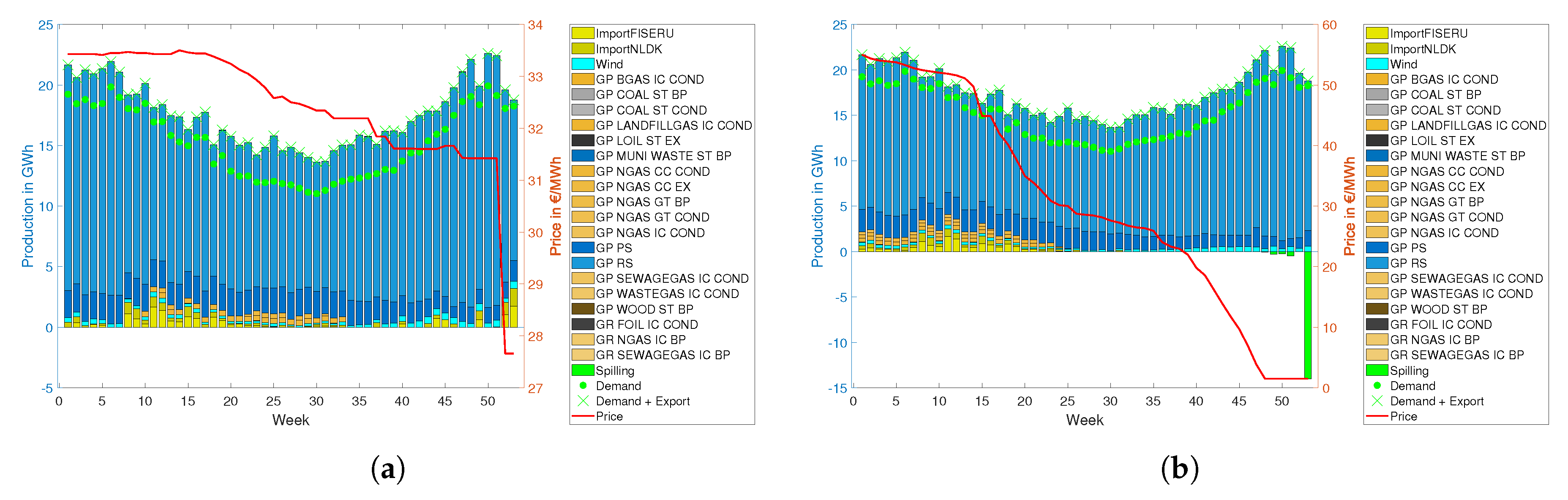
To keep the model comprehensible and fast, we took the following decisions. First of all, we aggregated all hours of the year into weekly representative time steps, as we want to analyse seasonal effects. All profiles (demand, wind, import, export, inflow) were averaged. The modelling horizon is one year. Furthermore, we aggregated the thermal power plants in terms of primary energy sources and power plant type. Moreover, all hydro power plants are aggregated into one reservoir power plant and one pumped storage power plant. We disregarded that Norway consists of five price zones and modelled Norway as one market area. Imports are modelled like power plants. Historical capacity limitations serve to restrict electricity imports and historical electricity prices in adjacent price zones represent the import costs. To obtain two representative import regions, we merged all price zones of Sweden, Finland and Russia into one representative import region as well as the Netherlands and the western price zone of Denmark into another one. For export, we decided to model it as a fixed curve added to the electricity demand curve instead. As there are only a few cogeneration of heat and power plants in Norway, we disregarded the heating market. In contrast, the reserve market in the Nordic countries is quite large, but we still neglect it here for simplicity reasons.
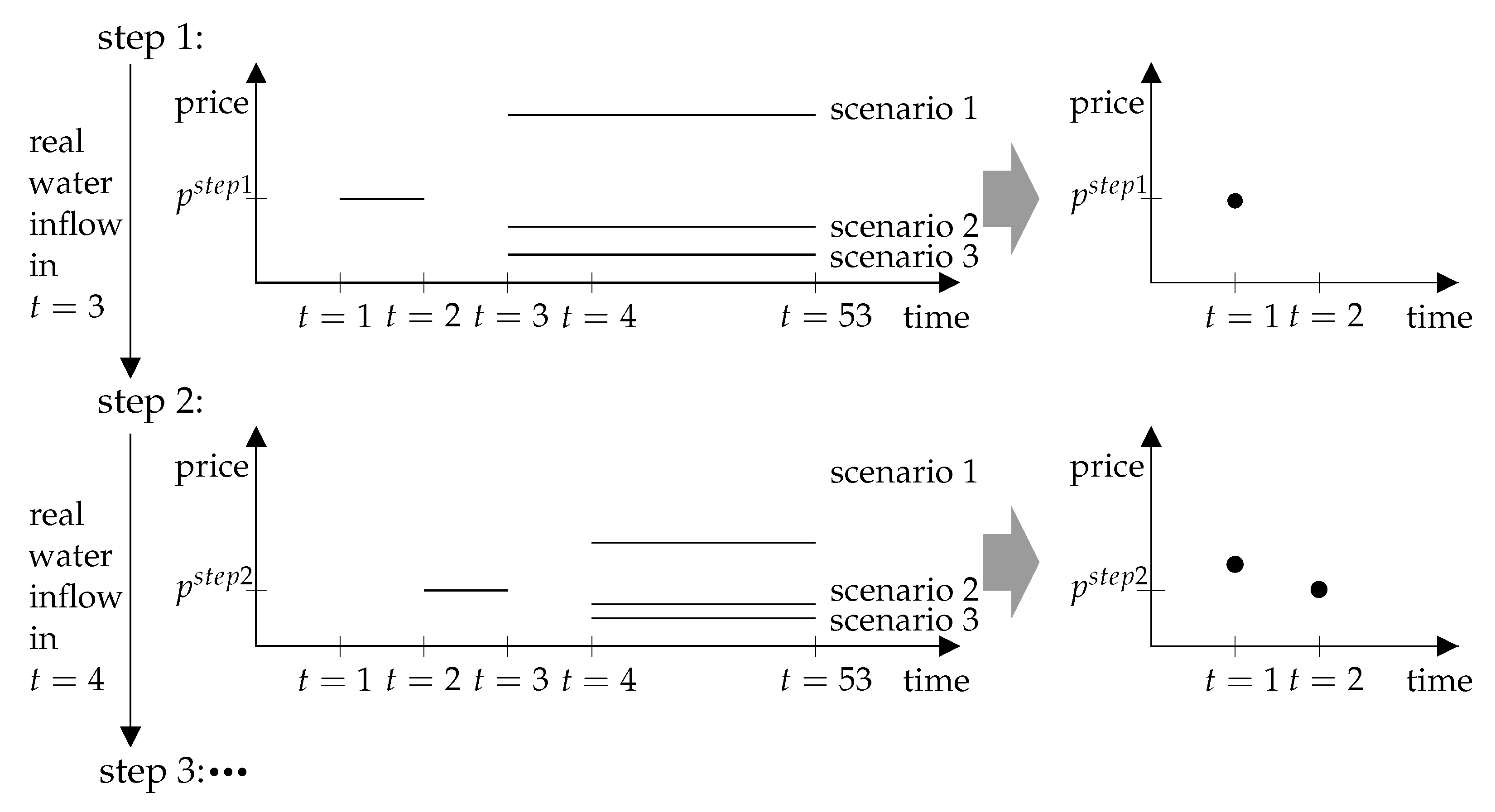
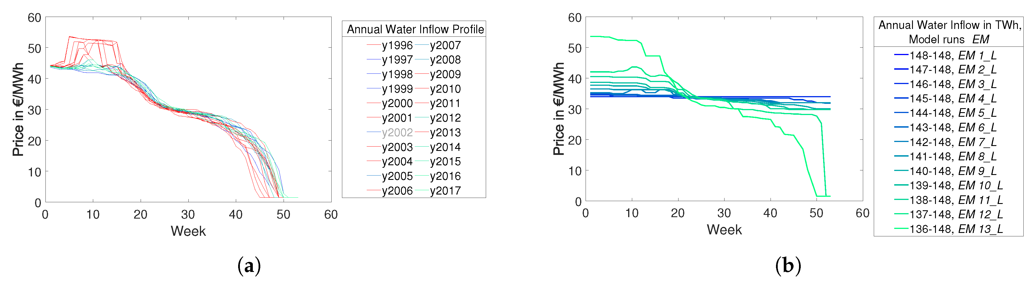
To include uncertainty regarding water inflow into the optimisation model, we used a second stage SDDP approach, with historic water inflow series for the optimisation scenarios and the simulation, based on the approach of [21,22]. The inflow can be predicted accurately for about one week [
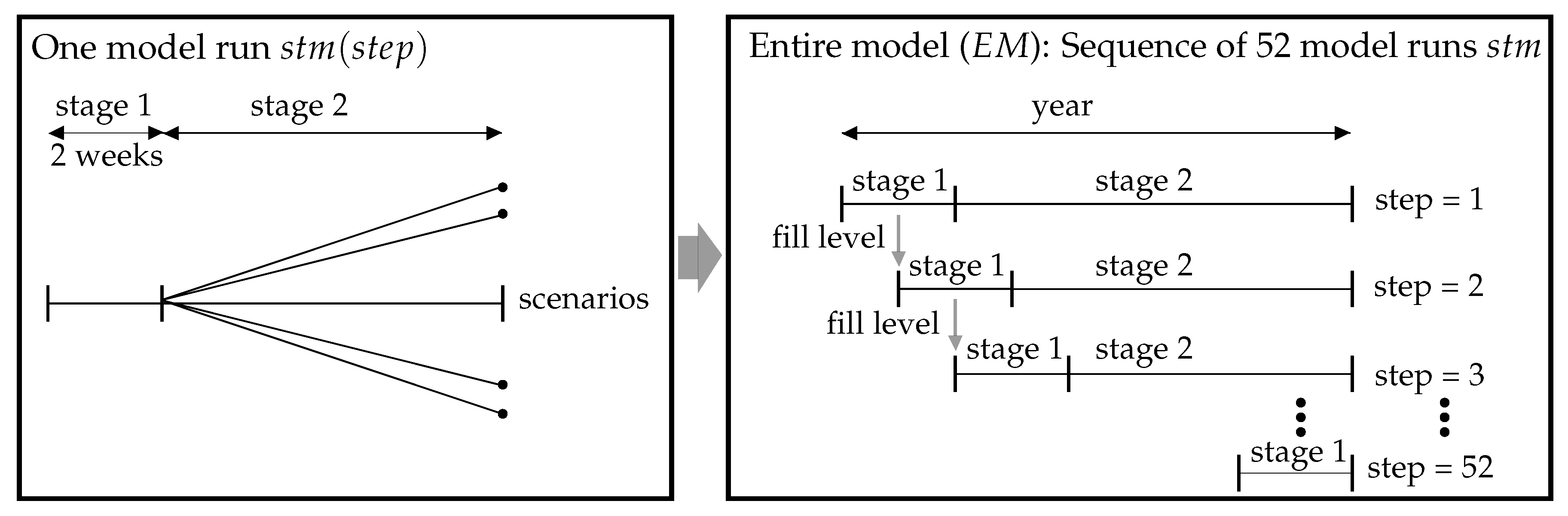
7]. As our model is based on weekly time steps, we need two weeks of stage one to get a unique dual variable (see below). Therefore, the first two weeks of a stochastic model run s t m correspond to stage one, whereas the following weeks of uncertain water inflow correspond to stage two (see Figure 1). With this approach, we underestimate at most the influence of uncertainty. Since we want to model a whole year and receive new information about the water inflow every week, we use a rolling horizon framework and therefore go successively through the year (see Figure 1).
As a result, our entire model E M consists of 52 stochastic model runs s t m . These model runs are determined by their starting week and are thus denoted with s t m ( s t e p ) where s t e p { 1 , , 52 } . For the first model run s t m ( s t e p = 1 ) , the initial fill levels are exogenously given. In contrast, the initial fill levels of all other model runs s t m are determined by the fill levels of the previous model runs. In a first approach, only the annual water inflow quantity is uncertain and we assume the water inflow profile to be known. The water inflow of stage 2 for every scenario ω Ω in a model run s t m ( s t e p ) is calculated as the product of a historic water inflow profile and a yearly amount of water inflow depending on the scenario ω :
WaterInflow ( t , ω ) = WaterInflowProfile ( t ) · AnnualWaterInflow ( ω )
for every time step t { s t e p + 2 , , 53 } . We specify the water inflow scenarios ω and their probabilities in Section 3. The water inflow of stage 1 for time steps t { s t e p , s t e p + 1 } is calculated in the same way, except that the annual water inflow does not depend on any scenario, but corresponds to the annual inflow of the realisation.
A more detailed and mathematical description of the stochastic model will be found in Appendix B.
For a standard linear optimisation problem without degeneracy and an existing, finite solution, we can interpret the dual variables as shadow prices. We will briefly discuss this in the following. Following the typical nomenclature, c denotes the cost vector, x the variables that are optimised (e.g., production, fill level) and A x b represents the linear restrictions (e.g., demand restriction, capacity restrictions). For more details, see Appendix A. The formulation of the primal problem of a linear optimisation model is:
min x c T x , s . t . A x b , x 0 ,
with x R k , c R k , b R m and A R m × k . The associated dual problem looks as follows:
max y b T y , s . t . A T y c , y 0 ,
with y R m . We define the optimum value depending on b as
z ( b ) : = min { c T x | A x b , x 0 } .
According to [23], the following equation holds in case of non-degeneracy:
z b i ( b ) = ( y * ) i ,
with y * signifying the optimal solution to the dual problem, and 1 i m denoting the i-th component of the corresponding vector. For a more detailed proof, see [23].
In the deterministic model, the dual variable of the demand restriction for each time step represents the electricity market price. The dual variable shows how the costs of the model change, when the electricity demand is marginally varied. Under the assumption of a market with perfect competition, the market participants will bid on the short-run marginal costs [24], which includes marginal opportunity costs for storages. The most expensive bid of the market participants corresponds to the dual variable in each time step. For the stochastic model E M , we always use the dual variable of week one of the demand equation of the model runs s t m . As we go in weekly steps through the year, we obtain an electricity price for each time step of the year.
All data are based on the Norwegian electricity market in 2017 (see Appendix C).
The general approach to analyse the effects of inflow uncertainty in this paper is outlined in the following. First, pricing in a deterministic model in a market with high shares of renewable energies is discussed. This forms the basis for understanding the price formation in the stochastic model and for comparing the results of both approaches. Then, the principle of price formation in a stochastic model is explained.
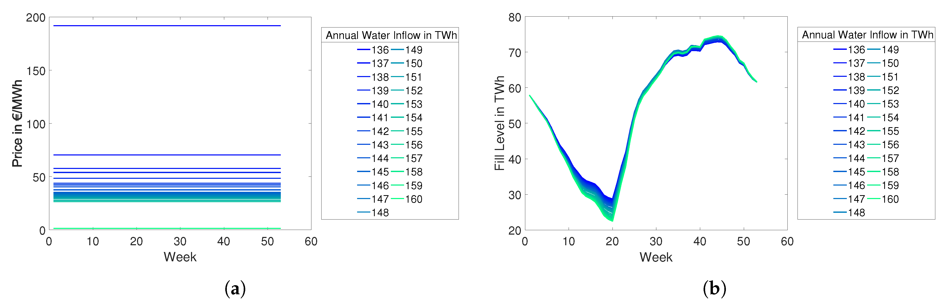
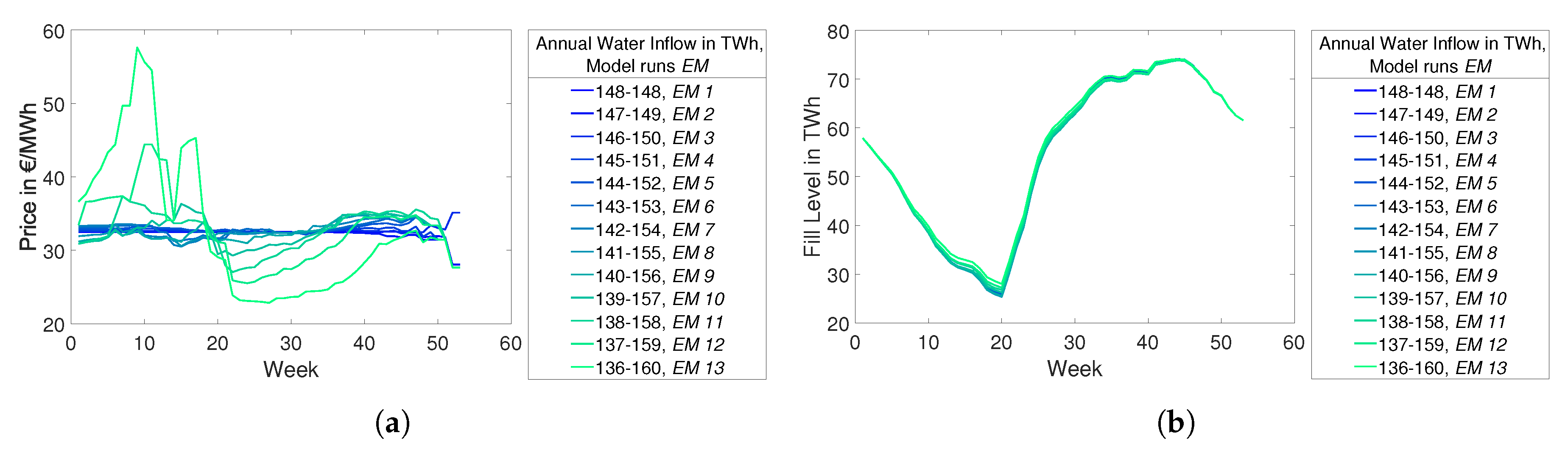
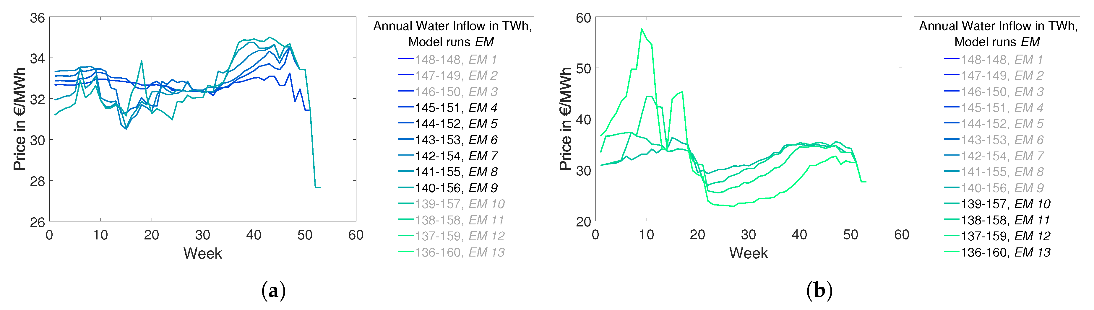
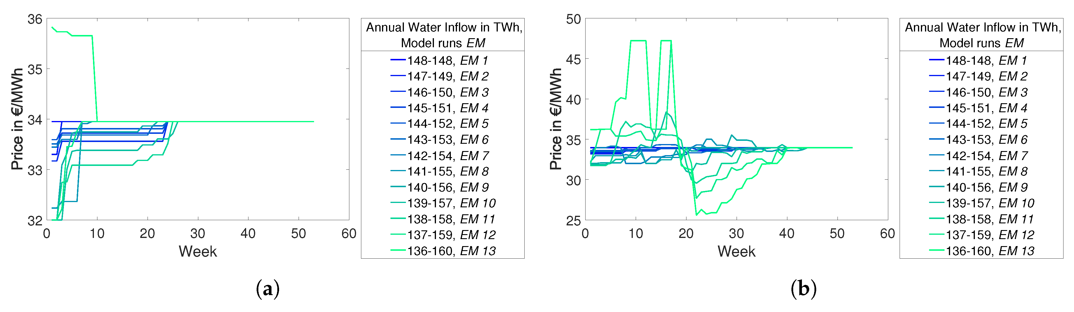
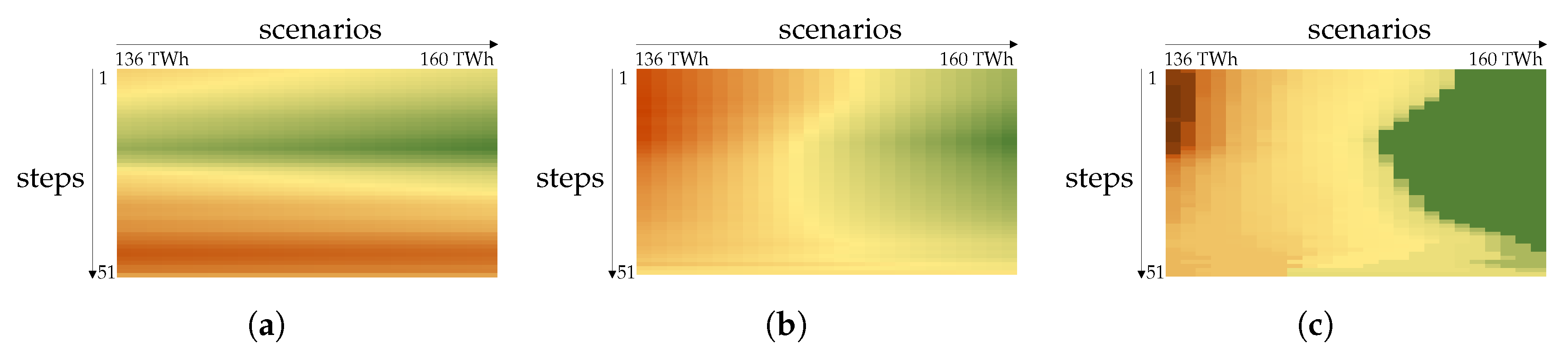
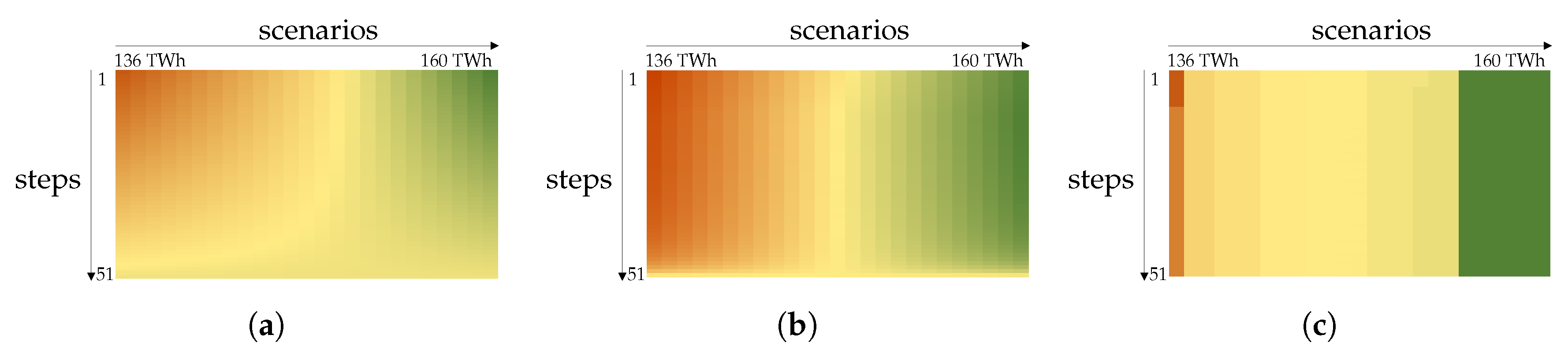
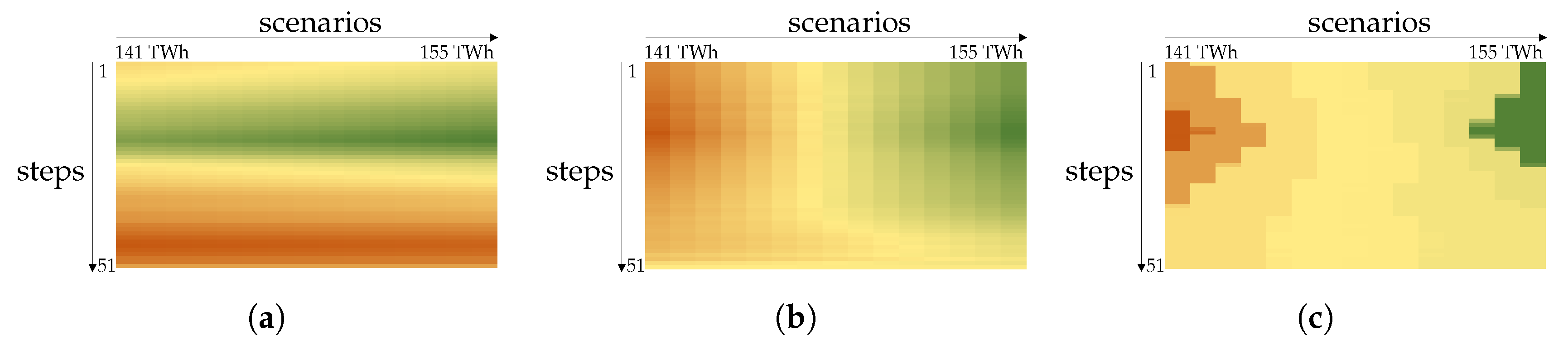
Subsequently, the influence of the inflow uncertainty is examined using the presented model. For this purpose, model runs with a different degree of uncertainty are compared. More precisely, this means that successively more scenarios are added to each model run E M , thus increasing the uncertainty. Hence, it can be determined what changes with increasing uncertainty and the reasons for this can be investigated. Three basic scenarios are defined for this purpose: (1) Less water is expected than inflows; (2) More water is expected than inflows; (3) The same amount of water is expected as inflow, i.e., the expected value of the water inflow of the scenarios corresponds to the real water inflow. In these three contrasting settings, the different modes of action and effects of uncertainty can be analysed well. In the first setting, we start with a model run E M that has only one inflow scenario and is therefore deterministic. Then, we add a second inflow scenario where the annual inflow is 1 TWh lower. In a third model run E M , a third scenario is added, where the annual water inflow is 1 TWh lower than the second scenario and so on. For the second setting, analogous inflow scenarios are added, which are each 1 TWh higher than the previous inflow scenario. In the third setting, two scenarios are successively added to each model run E M , each with 1 TWh less and 1 TWh more than the scenarios before. For all model runs, we assumed the probability of the inflow scenarios to be equally distributed.
Furthermore, for each of the settings, it is examined which previously made assumptions about profiles and costs in the model change the influence of uncertainty. These are in particular water inflow profiles, other profiles (demand, export and wind), and cost assumptions of power plants and import.
Finally, we compare our results to the actual Norwegian electricity price structure to evaluate them.

3. Results

The structure of this chapter follows the approach described in the methods section. The chapter starts with the explanation of price building mechanisms in deterministic and stochastic models. We then move on to analyse the effects of uncertainty using the presented model and approach.

3.1. Price Building in a Deterministic Model and Market with High Shares of Storages and Renewable Energies

For this subsection, we assume the water inflow to be known. If the market has a high share of renewable energies and the storage volume as well as the storage production capacity is very high, all prices in a modelled time segment are the same and equal to the marginal production costs or import of the most expensive production unit. Figure 2 shows an example that explains this phenomenon.
For simplicity, we assume that there are only four time steps and the demand can be met with three power plants. Each box in Figure 2 symbolises one unit of demand. There is one hydro power plant, one coal and one gas power plant, with associated marginal costs of 1 €/MWh, 20 €/MWh and 30 €/MWh (see Figure 2). In total, there are ten units of demand and hydro production is restricted to nine units of water (given in MWh). The hydro power storage has enough volume to contain all water units, which are given directly at the beginning of the year. Under these assumptions, a cost minimization with a demand restriction, a capacity and a storage balance restriction leads to an infinite number of solutions. Three of these optimal power plant commitment solutions are shown in Figure 2. In all three examples, the electricity prices are equal to 20 €/MWh, no matter when the coal power production takes place. This result makes sense for the following reasons. First, in case of non-degeneracy, the dual variable is unique and therefore the same in all three examples. Second, assuming the demand would marginally increase at any given time, this would in any case result in the need of more electricity production from the coal power plant. Therefore, the dual variable in each time step corresponds to the marginal costs of the coal-fired power plant. If the model had only five water units available, the gas-fired power plant would be needed to cover the entire demand. This would lead to a price of 30 €/MWh in each time step.
These findings also hold true with a more complex model (e.g., the deterministic model described in Section 2). This is clearly shown in Figure 3a. Prices are constant for each water inflow scenario, but differ in the absolute value. It is apparent that the price level is not linearly dependent on the annual water inflow. If the flexibility of the system is large enough, the price is determined by the (here yearly) energy gap, which must be covered by thermal power plants or imports. The storages are large enough and have enough production capacity to distribute the water wherever it is needed. Therefore, the opportunity costs of water, i.e., water values, always correspond to the marginal production costs of the most expensive power plant in the modelled time period minus the own (negligibly small) marginal production costs in all time steps.
As the storage operation also greatly influences the stochastic outcome, it is important to understand the storage operation for different annual inflow scenarios. Figure 3b shows that the storage fill levels follow a relatively similar course, but differ in altitude. This means that in deterministic model runs with high annual water inflows the reservoirs are emptier before the large water inflows in spring and then filled to a higher level than in model runs with low annual inflows. We want to emphasise that we only varied the amount of yearly inflow and left the inflow profile unmodified: WaterInflow ( t ) = WaterInflowProfile ( t ) · AnnualWaterInflow( s c e n a r i o s ).
If either capacity bounds or volume bounds of the storage are reached, prices no longer follow a constant course. It is not possible to produce “any” amount of electricity from water at all times. The water values therefore do not always correspond to the marginal production costs of the most expensive power plant or import at every time step. We will not cover this topic in this paper. In our case, with an aggregated hydro system, there are no availability factors for power plants, no reserve market and no additional restrictions for the fill levels of the storages (see Section 2 and Appendix A). The deterministic model prices are constant, regardless of the water inflow profile. We tested the impact of water inflow profiles on years 1996–2017. Only the water inflow profile of the year 2002 has an impact on the modelled electricity prices. An explanation will be found in Appendix D. Since price building mechanisms are different here, this year is not suited for the investigation of the impact and the comparison of profiles on electricity prices under uncertainty in the framework of this paper.

3.2. Principle Price Building Mechanisms in a Stochastic Model and Market with High Shares of Storages and Renewable Energies

To explain the general price building mechanisms, we use a generic example with three inflow scenarios (see Figure 4). Scenario 1 is the scenario with the lowest annual water inflow, scenario 2 has a higher inflow and scenario 3 is the one with the highest annual water inflow. The water inflow that realises successively from one s t e p to the next is the water inflow of scenario 3. The electricity price in each time step t = s t e p corresponds to the dual value of the demand restriction in time step t = s t e p in a model run s t m ( s t e p ) . As we go successively through the year, there is a price for each time step t { 1 , , 53 } . The dual variables of the demand restrictions in t = s t e p and t = s t e p + 1 (stage 1) corresponds to the expected value of the dual variables of the demand restrictions of the scenarios. For each stochastic scenario of a model run s t m ( s t e p ) , the prices are the same for all time steps t { s t e p + 2 , , 53 } and follow the price building mechanisms from Section 3.1. The level of the prices of the stochastic scenarios can differ for each model run s t m ( s t e p ) because of new information about the water inflow. This can result in different prices for each time step.

3.3. Impact of Long-Term Uncertainty on Electricity Prices

In this section, we analyse the impact of uncertainty on electricity prices. Although the same assumptions apply to the reservoirs in the deterministic and stochastic model, we obtain price trends that are not constant, if taking into account uncertainty. In the following, we show price curves obtained using uncertainty and explain the reasons for their structures.

3.3.1. Expectations of Less Water Inflow Than the One That Materializes

First of all, when comparing different model runs E M with different inflow scenarios, it is apparent that the impact of uncertainty on prices increases when more scenarios with less inflow are included into the optimisation (see Figure 5a).
It is prominent that the price in the first time step is not linearly dependent on the enclosure of inflow scenarios, which increase linearly. This is due to the fact that the dual variables of the demand restrictions in stage one corresponds to the expected value of the dual variables of the demand restrictions of the scenarios. The dual variables of each scenario are not linearly dependent on water inflow (see Figure 3). The main effect is that the prices are no longer constant, but decrease over the year. This is due to the fact that the expected water inflow increases over the year. This means that prices fall in all scenarios of a model run s t m ( s t e p ) and thus also in stage one. As typical water inflow profiles have their peak in summer weeks, the gradient of the price course is higher in summer weeks. This reasoning explains the higher starting points and the fall in prices, but not why they fall below the prices of the deterministic model run. Figure 5b shows that with increasing uncertainty the fill levels are higher. In expectation of dry years, more water is stored at the beginning of the year and therefore there is more electricity production from thermal power plants at the beginning of the year (see Figure 6). As a consequence, there is too much water left in the end of the year. In some of the more extreme model runs (e.g., model run 13), water spills over at the very end of the year.
Unlike in deterministic model runs, the underlying water inflow profile plays a role in stochastic model runs. One reason has already been mentioned, namely that the expected value of the inflow changes depending on the time step and the inflow in this time step. A second reason is that the main uncertainty dissolves in different time periods. For inflow profiles where the main water inflow comes late in the year, there is a longer period of (high) uncertainty. In that case, the difference of storage operation in stochastic model runs and deterministic model runs is higher compared to profiles where the main water inflow comes early in the year. This is due to the fact that even more water is stored at the beginning of the year in stochastic models if the main inflow comes late in the year. As a result, there is more water left at the end of the year in these cases, which leads to lower electricity prices towards the end of the year. Another effect is that the prices for some underlying water inflow profiles increase at the beginning of the year. This is unintuitive at first because the expected water inflow in this stetting increases at every time step (see Figure 7a). All profiles to which this applies are extremely low at the beginning of the year. This effect is caused by iterating successively through the year. In the extreme assumption that the profile is zero in some time steps, there is only one difference from s t m ( s t e p ) to s t m ( s t e p + 1 ) . In s t m ( s t e p ) , the fill level can be chosen individually for each scenario for the time step t = s t e p + 2 , whereas one uniform fill level must be chosen for all scenarios in time step t = s t e p + 2 in model run s t m ( s t e p + 1 ) . Therefore, a fill level “somewhere in the middle” is chosen for that time step in model run s t m ( s t e p + 1 ) . As a consequence, the dual variables of the scenarios with less inflow increase, whereas the scenarios with more inflow decrease slightly. In total, the mean value increases.
Additionally, the underlying structure of primary energy prices influences the course of electricity prices in a stochastic model. In Figure 5a, we assumed (historical) seasonal primary energy price structures. That means primary energy prices are lower in summer and higher in winter. To analyse the impact of detailed seasonal primary energy prices, we made the same calculations as in Figure 5a, but now with constant primary energy prices over the year (see Figure 7b). When comparing both figures, it is noticeable that electricity prices in Figure 5a fall more strongly towards the end of the year. If seasonal primary energy prices serve as data basis, the model produces more electricity from thermal power plants in summer, despite the inflow uncertainty. Hence, more water is available towards the end and electricity prices fall during this period.

3.3.2. Expectations of More Water Inflow Than the One That Materializes

If all water inflow scenarios are above the realizable water quantity, inverse price curves are obtained. The explanations are basically the same.

3.3.3. The Expected Value of Water Inflow Corresponds to the One That Materializes

If the realizing water inflow corresponds exactly to the expected value of all inflow scenarios, the electricity price profile is clearly seasonal for all model runs E M with higher uncertainty (see Figure 8a). The seasonal structure becomes more pronounced the higher the uncertainty.
In the first three model runs E M , where the first run is deterministic, there is hardly any price variation. Conversely, the model runs E M 4–9 (see Figure 9a) and 10–13 (see Figure 9a,b) definitely differ from the deterministic model run. The model runs E M 4–9 show a higher elevation at the end of the year, whereas the highest elevation of the model runs E M 10–13 is located at the beginning of the year. In the following, we explain the seasonal shape of electricity prices and the differences between the model runs shown in Figure 9a,b.
One aspect is that the prices do not depend linearly on the water inflow (see Section 3.1). This is the reason for all starting points in Figure 8b to differ from each other.
The seasonal price shape strongly depends on the seasonal water inflow profile, demand profile and export profile as well as seasonal primary energy prices and import prices. Without these seasonal profiles, there is no seasonality in electricity prices (see Figure 10a).
We begin to analyse the reason for seasonal price trends by means of a slightly simpler problem. Water inflow, demand, export and wind are still modelled via seasonal profiles but primary energy prices and import are assumed to be constant (see Figure 10b).
As stated in Section 3.1, prices are the same in each time step t { s t e p + 2 , , 53 } for a scenario in one model run s t m ( s t e p ) . The price level is dependent on the ratio of demand, export, wind, water inflow as well as start and end fill levels for each time frame of s t m ( s t e p ) . This means prices are dependent on the energy gap in the modelled time frame, which has to be met by thermal power plants and import. Since we model different thermal power plants with different costs, prices also depend on the capacity from thermal power plants and import which is available for the time period to be modelled. We define two ratios which help to explain the observed effects. The first one is independent of any model output and represents the ratio of demand, export, wind, water inflow and thermal capacity and import for the modelled time frame:
ratio 1 ( s t e p , s c e n a r i o ) = DemandRestYear ( s t e p , s c e n a r i o ) + ExportRestYear ( s t e p , s c e n a r i o ) ThermalCapacityAndImportRestYear ( s t e p ) + WindRestYear ( s t e p , s c e n a r i o ) WaterInflowRestYear ( s t e p , s c e n a r i o ) ThermalCapacityAndImportRestYear ( s t e p ) .
Figure 11a shows a heat map for r a t i o 1 for all scenarios, which are plotted on the horizontal axis and (model) steps, which are plotted on the vertical axis. We can clearly identify that with a seasonal shape of demand, export, wind and water inflow r a t i o 1 changes in a (different) seasonal curve over the year for each scenario.
In a second ratio ( r a t i o 2 ), we take the results of the model runs s t m ( s t e p ) into account and include the start and end fill levels for each model run s t m ( s t e p ) :
ratio 2 ( s t e p , s c e n a r i o ) = ratio 1 ( s t e p , s c e n a r i o ) + startfilllevel ( s t e p ) + endfilllevel ( s t e p ) ThermalCapacityAndImportRestYear ( s t e p ) .
In addition, including the storage operation, the seasonal shape of Figure 11a is levelled out, especially for the middle scenarios (see Figure 11b). Towards the end, all ratios equalize, as uncertainty resolves. However, a clear difference can now be seen between the individual scenarios. In addition, there is still a subdued seasonal structure of r a t i o 2 in each column, although the seasonal structure is a little more pronounced in the more extreme scenarios.
We assume for a moment that we had deterministic model runs with the corresponding annual water inflows of the scenarios. This would lead to higher values for r a t i o 2 in low inflow scenarios and lower values for r a t i o 2 in high inflow scenarios. Still, there would be the same value for r a t i o 2 in every column. In the deterministic model, the storage can balance the seasonality of a year completely for each separate scenario. In contrast, in the stochastic model E M , the storage is not able to balance equally each different seasonal structure of r a t i o 1 of each scenario. This is due to the fact that the model has to find unique fill levels for the first two weeks for all scenarios. In contrast, with constant profiles and prices, the reservoirs do not need to compensate for seasonal structures (see Appendix E.1). If there are no seasonal structures in r a t i o 1 , they do not need to be balanced and therefore no seasonal structures exist in r a t i o 2 . As a consequence, there are also no seasonal price structures for the individual scenarios and as a result there is also no seasonal price structure in the modelled electricity prices (see Figure 10a).
Depending on the chosen scenarios and the cost structure, the uniform fill level will tend to either side (see Figure 8b). The fill level of the model runs E M 4–9 is lower than the fill levels of the model runs E M 10–13 before the main water inflow in spring. In that time period, the impact of scenarios with high water inflow is stronger than scenarios with low water inflow for the model runs E M 4–9. For model runs E M 10–13, this is the other way round.
The prices of the stochastic scenarios correspond to r a t i o 2 (see Figure 11c). Together, the mean values of the rows in Figure 11c result in the price curve of model run E M 13 in Figure 10b. It is obvious that the high prices at the beginning of the year are determined by the first scenarios with low water inflow. In contrast, low prices in the middle of the year are caused through the dominance of the last scenarios with high water inflow. This provides the explanation for the price curve of model run E M 13 in Figure 10b as well as the principle price elevation at the beginning of the year and deepening in the middle of the year of model run E M 13 in Figure 9b. We have already mentioned that the storage operation is different for all 13 model runs E M of Figure 8b. Therefore, also r a t i o 2 and the prices for each scenario differ from Figure 11b,c. However, they do not differ much (see Appendix E.2). Hence, conclusions for other model runs can be drawn from Figure 11c. Leaving aside the four outer scenarios, the low prices of scenarios 16–21 are getting dominant and cause the deepening of prices in Figure 9b and Figure 10b between weeks 15 and 35.
Seasonal primary energy prices intensify the seasonal structure of electricity prices when uncertainty is included into the modelling. The same r a t i o 2 for model runs E M with and without seasonal primary energy prices would still lead to different electricity prices. Primary energy prices are more expensive in winter weeks. Therefore, the same ratio leads to higher prices in the winter time and lower prices in the summer. In fact, the ratios are not the same because more electricity is produced from thermal power plants in summer when prices for primary energy sources are more favourable (see also Section 3.3.1). Nevertheless, the structure of r a t i o 2 is similar.
As r a t i o 1 has an impact on the prices, so do the underlying water inflow profiles. All historical water inflow profiles are seasonal and therefore cause seasonal electricity price shapes. According to their own specific inflow profiles, the resulting price profiles differ from the ones shown here.
If the actual water inflow does not correspond exactly to the mean value of the inflow scenarios, seasonal price trends are still apparent. This is also the case if all scenarios are either rather dry or wet, whereas the seasonal structure is less pronounced for wet water inflow scenarios.

3.3.4. Comparison to Norwegian Price Pattern

Looking at historical Norwegian price trends between the years 2008 and 2017, the similarity to the price trends presented in this paper becomes apparent (see Figure 12 and Figure 13). Figure 12a shows similar price curves as in Section 3.3.1 and Figure 12b and Figure 13a resemble the modelled price curves of Section 3.3.3. Comparing the model results to the price curve of the year 2017 which defines the basic setting of the presented model, it becomes visible that the first price peaks as well as the plunge of prices during the weeks 20 and 30 can be captured (see Figure 13b). The model is not made for realistic price forecasts for several reasons which will be discussed in Section 4. However, it is suitable to show the importance and impact of including uncertainty into the optimisation when modelling prices with optimisation models in markets with a high share of renewable energies and storages.

4. Discussion

In Section 3.3.4, we have shown that the model is suitable to explain general seasonal price structures in the Norwegian market, but not to forecast prices in a realistic way. This has several reasons. For a more detailed and realistic price forecast, a more complex model, including, e.g., a detailed hydro system, a temperature-dependent demand and more differentiated costs structures including costs for demand response (see [17]) is necessary. Moreover, the assumption that the water inflow can be perfectly predicted for two weeks and is completely uncertain for the following weeks is probably not very realistic. However, the chosen simplifications help to better understand principle price building mechanisms and the impact of selected factors on the modelled prices under uncertainty. The analyses made here serve to identify principal effects and roughly quantify their magnitude.
Still, the question remains whether the basic results of this paper remain true when using a more complex model. Including a detailed hydro system as well as availabilities for hydro power plants and a reserve market into the modelling leads to a slightly different price building mechanism. However, this is not subject of this paper but would be interesting for future work. Nevertheless, we expect the effects shown in this paper to remain roughly the same even if the above factors are taken into account.
The fact that we only modelled one year with fixed end fill levels will probably strongly influence the last modelled weeks of the year. Therefore, we made some exemplary calculations on a longer modelling horizon. We used the same method as in Section 2 but extended the time horizon. For the longer time horizon, we used the data of the same year in succession. This results in a subdued seasonal pattern for the first modelled years. This outcome is caused by the fact that the change in inflow is smaller in relation to the total energy quantities and therefore has a smaller impact. We also made an approach for a longer time horizon for model runs E M where in each model run s t m ( s t e p ) the modelling horizon is one year. In this setting, the seasonal structures were not subdued, but were different from the ones shown here. This is due to the fact that in each model run s t m ( s t e p ) there is not only new information about the water inflow, but also about the last modeled time step (e.g., demand, end fill level) which change the ratio of energy quantities. Further research should be done on this subject.
The modelling approach with fixed start and end fill levels also leads to the problem that not all historical water inflows that have occurred can be modelled. We therefore chose a more generic approach and considered all annual water inflows that are feasible.
We assumed the amount of annual water inflow to be linearly distributed, which is approximately true except for the lower limit. Hence, we rather underestimate the effect of uncertainty in this point.
The influence of different underlying water inflow profiles is, in reality, probably less pronounced, as they can be balanced by the export profile, which is fixed in our modelling approach.
On the other hand, including uncertainty regarding water inflow profiles into the modelling would affect our results. It is reasonable to assume that this increases the influence of uncertainty, but further research should be done to understand in which way.
Although some research questions remain open, we believe that the basic mechanisms and effects remain correct and provide a good basis for further investigations.

5. Conclusions

We have shown that electricity market prices modelled with a deterministic optimisation model are constant in markets with high shares of renewable energies and storages. Including uncertainty into the modelling results in price structures that significantly differ from constant prices. The price structures become more pronounced the more uncertain the renewable energy feed-in is. Most price structures observed are clearly seasonal, except for those where the realised inflow is at the margin of expected annual water inflow. Uncertainty has an impact on electricity market prices even with constant inflow, demand, export and wind profiles. However, seasonal electricity price structures are caused by seasonal inflow, demand, export and wind profiles. These effects are reinforced by seasonal primary energy source prices and import prices.
We see similar price structures also in the historical Norwegian prices. Therefore, we conclude that taking into account uncertainty improves the price modelling with optimisation models.
Based on the analyses made, we conclude that the basic pricing mechanisms also apply to other uncertainties regarding wind, sun or demand. These uncertainties also have seasonal profiles and generate non-constant price structures depending on their share in the system and the size of the uncertainty. We believe that the influence of these uncertainties, especially wind in connection with Norway’s storage facilities, will play an increasingly important role. To estimate the magnitude of the influence, further investigations would have to be made.

Author Contributions

Conceptualization, H.S.; methodology, H.S.; software, H.S.; validation, H.S.; formal analysis, H.S.; investigation, H.S.; resources, H.S.; data curation, H.S.; writing—original draft preparation, H.S.; writing—review and editing, H.S., N.K. and K.H.; visualization, H.S.; supervision, N.K. and K.H. All authors have read and agreed to the published version of the manuscript.

Funding

This research was funded by German Federal Ministry of Education and Research (BMBF) within the Kopernikus project: Energy Transition Navigation System (ENavi) Grant No. 03SFK4M1.

Conflicts of Interest

The authors declare no conflict of interest.

Appendix A. Deterministic Model

We describe the mathematical formulation of the deterministic model in the following. The objective function looks as follows:
min x R + n c T x ,
where x R + n is a vector with
x = ( x P , x I , x P u m p , x F , x S )
and c R + n a vector with
c = ( c P , c I , c P u m p , 0 , 0 ) .
Table A1. Indices and sets.
IndicesSets
n T number of all time steps T : = { 1 , , 53 } set of all time steps
n P P number of all power plants P P set of all power plants
n C number of all import countriesC - set of all import countries
n H P P number of all hydro power plants H P P set of all hydro power plants
n : = n P P · n T + n C · n T + 3 · n H P P · n T
Table A2. Variables.
Vectors of VariablesVariables (Vector Entries)
x p R + n P P · n T electricity production x p ( p p , t ) R + electricity production of a specific power plant p p P P in time step t T
x I R + n C · n T electricity import x I ( c , t ) R + electricity import of a specific country c C in time step t T
x P u m p R + n H P P · n T pumped electricity x P u m p ( h p p , t ) R + electricity production of a specific hydro power plant h p p H P P in time step t T
x F R + n H P P · n T storage fill levels x F ( h p p , t ) R + storage fill level of a specific hydro power plant h p p H P P in time step t T
x S R + n H P P · n T spilling x S ( h p p , t ) R + spilling a specific hydro power plant h p p H P P in time step t T
Table A3. Costs.
Table A3. Costs.
Vectors of CostsCosts (Vector Entries)
c p R + n P P · n T costs for production c p ( p p , t ) R + electricity production costs of a specific power plant p p P P in time step t T
c I R + n C · n T electricity import costs c I ( c , t ) R + electricity import costs of a specific country c C in time step t T
c P u m p R + n H P P · n T costs of pumped electricity c P u m p ( h p p , t ) R + costs of electricity production of a specific hydro power plant h p p H P P in time step t T
In our case, production costs include variable operation and maintenance costs ( c V O a M ( p p ) ), fuel costs ( c F u e l ( p p , t ) ) and CO2 costs ( c C O 2 ( p p , t ) ) for the electricity production:
c P ( p p , t ) = c V O a M ( p p ) + c F u e l ( p p , t ) + c C O 2 ( p p , t ) p p P P , t T
with
c F u e l ( p p , t ) = TimeWeight ( t ) · PrimaryEnergyPrice ( p p , t ) MaxEfficiency ( p p )
and
c C O 2 ( p p , t ) = TimeWeight ( t ) · CO 2 Factor ( p p ) · CO 2 Price ( t ) MaxEfficiency ( p p ) .
We use the parameter T i m e W e i g h t as a weight because of the representative weekly time steps. The weight is chosen as follows: T i m e W e i g h t ( t ) = 168 t { 1 , , 52 } and T i m e W e i g h t ( t ) = 24 for t = 53 . Moreover, the parameter P r i m a r y E n e r g y P r i c e is based on historical prices (see Table A4 for the source) and M a x E f f i c i e n c y ( p p ) is the linearized efficiency for each power plant. The CO2 factor ( C O 2 F a c t o r ( p p ) ) denotes the emission intensity. The costs of import correspond to the historical wholesale power prices in the modelled countries (see Table A4). Additionally, we gave pumping little costs ( c P u m p ( h p p , t ) ) to avoid synchronous turbining and pumping instead of spilling.
The minimization problem is subject to the following restrictions:
  • Demand restriction:
    x P ( p p , t ) + x I ( c , t ) = Demand ( t ) + Export ( t ) Windproduction ( t ) p p P P , c C and t T ,
  • Capacity restrictions:
    x P ( p p , t ) Capacity ( p p ) p p P P , t T ,
  • Import restrictions:
    x I ( c , t ) AmountImport ( c , t ) c C , t T ,
  • Storage restrictions:
    x F ( h p p , t + 1 ) = x F ( h p p , t ) x P ( h p p , t ) + x P u m p ( h p p , t ) x S ( h p p , t ) + WaterInflow ( t ) h p p H P P , t { 1 , , 52 } ,
  • Initial fill level:
    x F ( h p p , t = 1 ) = Filllevelbegin ( h p p ) h p p H P P ,
  • End fill level:
    FilllevelEnd ( h p p ) = x F ( h p p , t = 53 ) x P ( h p p , t = 53 ) + x P u m p ( h p p , t = 53 ) x S ( h p p , t = 53 ) + WaterInflow ( t = 53 ) h p p H P P ,
  • Fill level restrictions
    x F ( h p p , t ) Filllevelboundary ( h p p ) h p p H P P , t T .

Appendix B. Stochastic Model

To model the uncertainty, we can use the extensive form of a second stage optimisation problem because the number of annual inflow scenarios is finite and therefore the support of the random vector is also finite [25].
In the following, we describe the mathematical formulation of a model run s t m ( s t e p ) , where s t e p { 1 , , 52 } .
The objective function for the stochastic model looks as follows:
min x s t a g e 1 , x s t a g e 2 { c T x s t a g e 1 + ω p ( ω ) c T x s t a g e 2 ( ω ) } ,
where ω Ω is a random event and Ω the event space. The factor p ( ω ) denotes the probability of a random event ω . The vector x s t a g e 1 corresponds to the vector x from the deterministic model (see Appendix A) except that, in contrast to the deterministic model, it only contains variables that are dependent on the two representative time steps t s t a g e 1 = s t e p and t s t a g e 1 = s t e p + 1 . In the same way, the vector x s t a g e 2 also corresponds in principle to the vector x from the deterministic model. However, the vector x s t a g e 2 only contains variables depending on representative time steps t s t a g e 2 { s t e p + 2 , , 53 } . Additionally, the variables are dependent on the random event/scenario ω . The cost vector c T does not change in comparison to the deterministic case and remains the same for stage one variables and stage two variables.
The restrictions of the first stage are the same as in Section 2. The only differences are that the equations here only apply to the time steps t s t a g e 1 { s t e p , s t e p + 1 } and that the initial fill levels for all model runs s t m with s t e p { 2 , , 52 } depend on the previous model run:
x F s t a g e 1 ( h p p , t = s t e p ) = x F F i l l L e v e l F r o m _ s t m ( s t e p 1 ) s t a g e 1 ( h p p , t = s t e p ) h p p H P P .
The storage restriction is the only cross-time equation between stage 1 and stage 2:
x F ( h p p , t s t a g e 2 , ω ) = x F ( h p p , t s t a g e 1 ) x P ( h p p , t s t a g e 1 ) + x P u m p ( h p p , t s t a g e 1 ) x S ( h p p , t s t a g e 1 ) + WaterInflow ( t s t a g e 1 ) h p p H P P , t s t a g e 1 = s t e p + 1 , t s t a g e 2 = s t e p + 2 and ω Ω .
The restrictions for stage two look as follows:
  • Demand restriction:
    x P s t a g e 2 ( p p , t s t a g e 2 , ω ) + x I s t a g e 2 ( c , t s t a g e 2 , ω ) = Demand ( t s t a g e 2 ) + Export ( t s t a g e 2 ) Windproduction ( t s t a g e 2 ) , p p P P , c C , t s t a g e 2 { s t e p + 2 , , 53 } and ω Ω
  • Capacity restrictions:
    x P s t a g e 2 ( p p , t s t a g e 2 , ω ) Capacity ( p p ) p p P P , t s t a g e 2 { s t e p + 2 , , 53 } and ω Ω ,
  • Import restrictions:
    x I s t a g e 2 ( c , t s t a g e 2 , ω ) AmountImport ( t s t a g e 2 ) c C , t s t a g e 2 { s t e p + 2 , , 53 } and ω Ω ,
  • Storage restrictions:
    x F s t a g e 2 ( h p p , t + 1 , ω ) = x F S t a g e 2 ( h p p , t s t a g e 2 , ω ) x P s t a g e 2 ( h p p , t s t a g e 2 , ω ) + x P u m p s t a g e 2 ( h p p , t s t a g e 2 , ω ) x S s t a g e 2 ( h p p , t s t a g e 2 , ω ) + WaterInflow ( t s t a g e 2 , ω ) h p p H P P , t s t a g e 2 { s t e p + 2 , , 53 } and ω Ω ,
  • End fill level:
    FilllevelEnd ( h p p ) = x F s t a g e 2 ( h p p , t = 53 , ω ) x P s t a g e 2 ( h p p , t = 53 , ω ) + x P u m p s t a g e 2 ( h p p , t = 53 , ω ) x S s t a g e 2 ( h p p , t = 53 , ω ) + WaterInflow ( t = 53 , ω ) h p p H P P and ω Ω
  • Fill level restrictions
    x F s t a g e 2 ( h p p , t s t a g e 2 , ω ) Filllevelboundary ( h p p ) h p p H P P , t s t a g e 2 { s t e p + 2 , , 53 } and ω Ω .

Appendix C. Data

Table A4. Data.
Table A4. Data.
DataSourceProcessing
electricity demandNord Pool Spotweekly average, sum of Norwegian price areas
exportNord Pool Spotweekly average, sum of all export from Norwegian price areas into external price areas/ countries
wind productionNVEweekly average, sum of all wind power plant production
water inflow NorwayNord Pool Spotgiven in calendar weeks, weekly average of the model weeks
water inflow power plantNVEaverage yearly water inflow recalculated into a ratio and multiplied with the Norwegian water inflow
start and end fill levelNord Pool Spotnone
import amount and pricesNord Pool Spotweekly average and average over the cumulated areas described above
hydro power plant dataNVEaggregated into a pump storage power plant and a reservoir power plant
thermal power plantsPlatts 2014categorized/aggregated after primary energy carrier and technology type
maximal electrical efficiency[26]averaged over age categories
primary energy prices[26]weekly average if not already in yearly or weekly form
Variable OaM costs[26]none
CO2 priceEEXweekly average
CO2 factor[27]none

Appendix D. Impact of the Profile of the Year 2002

The profile of the year 2002 has an extremely low inflow at the end of the year (see Figure A1a). The modelled reservoir was not able to store the spring inflow for the end of the year (see Figure A1b). This can be explained in particular by reservoir capacity and the assumption about fixed initial and end fill levels as well as export, which are based on the data of 2017.
Figure A1. Reasons for special prices under the water inflow profile of the year 2002. (a) inflow profiles; (b) storage operation and electricity price.
Energies 13 02347 g0a1

Appendix E. Ratios and Prices

Appendix E.1. All Profiles and Primary Energy Source Prices and Import Prices Are Constant

Figure A2. Ratios and prices for Figure 10a, model run EM 13 (Scenarios: 136 TWh–160 TWh), where all profiles and prices are constant. (a) ratio 1; (b) ratio 2; (c) scenario prices.
Energies 13 02347 g0a2

Appendix E.2. Historic Profiles and Constant Primary Energy Source Prices and Import Prices

Figure A3. Ratios and prices for Figure 10b for model run EM 8 (Scenarios: 141 TWh–155 TWh). (a) ratio 1; (b) ratio 2; (c) scenario prices.
Energies 13 02347 g0a3

References

  1. Nord Pool. Available online: ftp://ftp.nordpoolgroup.com/ (accessed on 1 March 2019).
  2. Helseth, A.; Haugen, M.; Jaehnert, S.; Mo, B.; Farahmand, H.; Naversen, C. (Eds.) Multi-Market Price Forecasting in Hydro-Thermal Power Systems; IEEE: New York, NY, USA, 2018. [Google Scholar]
  3. Grote, F.; Maaz, A.; Drees, T.; Moser, A. Modeling of electricity pricing in European market simulations. In Proceedings of the IEEE 2015 12th International Conference on the European Energy Market (EEM), Lisbon, Portugal, 19–22 May 2015; pp. 1–5. [Google Scholar] [CrossRef]
  4. Ward, K.R.; Green, R.; Staffell, I. Getting prices right in structural electricity market models. Energy Policy 2019, 129, 1190–1206. [Google Scholar] [CrossRef]
  5. Pape, C.; Hagemann, S.; Weber, C. Are fundamentals enough? Explaining price variations in the German day-ahead and intraday power market. Energy Econ. 2016, 54, 376–387. [Google Scholar] [CrossRef] [Green Version]
  6. Spiecker, S.; Vogel, P.; Weber, C. Evaluating interconnector investments in the north European electricity system considering fluctuating wind power penetration. Energy Econ. 2013, 37, 114–127. [Google Scholar] [CrossRef]
  7. Wallace, S.W.; Fleten, S.E. Stochastic Programming Models in Energy. In Stochastic Programming; Handbooks in Operations Research and Management Science; Elsevier: Amsterdam, The Netherlands, 2003; Volume 10, pp. 637–677. [Google Scholar] [CrossRef]
  8. Gjelsvik, A.; Mo, B.; Haugstad, A. Handbook of Power Systems I: Long- and Medium-term Operations Planning and Stochastic Modelling in Hydro-dominated Power Systems Based on Stochastic Dual Dynamic Programming; Springer: Berlin/Heidelberg, Germany, 2010. [Google Scholar] [CrossRef]
  9. Iliadis, N.A.; Tilmant, A.; Chabar, R.; Granville, S.; Pereira, M. Optimal operation of hydro-dominated multireservoir systems in deregulated electricity markets. In Proceedings of the International Conference for Reservoir Operation and River Management, Guanghzou, China, 17–23 September 2005. [Google Scholar]
  10. Jaehnert, S.; Doorman, G.L. Assessing the benefits of regulating power market integration in Northern Europe. Int. J. Electr. Power Energy Syst. 2012, 43, 70–79. [Google Scholar] [CrossRef]
  11. Flatabo, N.; Haugstad, A.; Mo, B.; Fosso, O.B. Short-term and Medium-term Generation Scheduling in the Norwegian Hydro System under a Competitive Power market Structure. In Proceedings of the International Conference on Electrical Power Systems Operation and Management, ETH Zürich, Switzerland, 23–25 September 1998. [Google Scholar]
  12. Botnen, O.J.; Johannesen, A.; Haugstad, A.; Kroken, S.; Froysteil, O. Modelling of hydropower scheduling in a national/ international context. In Hydropower ’92; CRC Press: Boca Raton, FL, USA, June 1992. [Google Scholar]
  13. Pereira, M.V.F. Optimal Scheduling of Hydrothermal Systems—An Overview. IFAC Proc. Vol. 1985, 18, 1–9. [Google Scholar] [CrossRef]
  14. Pereira, M. Long-term Hydro Scheduling based on Stochastic Models. In Proceedings of the International Conference on Electrical Power Systems Operation and Management, ETH Zürich, Switzerland, 23–25 September 1998; Available online: https://scholar.google.de/scholar?q=pereira+Long-term+Hydro+Scheduling+based+on+Stochastic+Models&hl=en&as_sdt=0&as_vis=1&oi=scholart (accessed on 7 May 2020).
  15. Wolfgang, O.; Haugstad, A.; Mo, B.; Gjelsvik, A.; Wangensteen, I.; Doorman, G. Hydro reservoir handling in Norway before and after deregulation. Energy 2009, 34, 1642–1651. [Google Scholar] [CrossRef]
  16. Aouam, T.; Yu, Z. Multistage Stochastic hydrothermal scheduling. In Proceedings of the 2008 IEEE International Conference on Electro/Information Technology, Ames, IA, USA, 18–22 May 2008; pp. 66–71. [Google Scholar]
  17. Haugstad, A.; Rismark, O. Price Forecasting in an Open Electricity Market based on System Simulation. In Proceedings of the International Conference on Electrical Power Systems Operation and Management, ETH Zürich, Switzerland, 23–25 September 1998. [Google Scholar]
  18. Maceira, M.; Duarte, V.; Penna, D.; Moraes, L.; Melo, A. Ten years of application of stochastic dual dynamic programming in official and agent studies in Brazil—Description of the NEWAVE program. In Proceedings of the 16th Power Systems Computation Conference, Glasgow, Scotland, 14–18 July 2008. [Google Scholar]
  19. Gjerden, K.S.; Helseth, A.; Mo, B.; Warland, G. (Eds.) Hydrothermal Scheduling in Norway Using Stochastic Dual Dynamic Programming; A Large-Scale Case Study; IEEE: New York, NY, USA, 2015. [Google Scholar]
  20. Pereira, M.V.F.; Pinto, L.M.V.G. Multi-stage stochastic optimization applied to energy planning. Math. Program. 1991, 52, 359–375. [Google Scholar] [CrossRef]
  21. Helseth, A.; Mo, B.; Warland, G. Long-term scheduling of hydro-thermal power systems using scenario fans. Energy Syst. 2010, 1, 377–391. [Google Scholar] [CrossRef]
  22. Helseth, A.; Mo, B.; Lote Henden, A.; Warland, G. Detailed long-term hydro-thermal scheduling for expansion planning in the Nordic power system. IET Gener. Transm. Distrib. 2018, 12, 441–447. [Google Scholar] [CrossRef] [Green Version]
  23. Burkard, R.E.; Zimmermann, U.T. Einführung in die Mathematische Optimierung; Springer: Berlin/Heidelberg, Germany, 2012; Volume 5045. [Google Scholar] [CrossRef]
  24. Fundamental Market Models. In Managing Energy Risk; John Wiley & Sons, Ltd.: Hoboken, NJ, USA, 2014; pp. 301–391. [CrossRef]
  25. Birge, J.R.; Louveaux, F. Introduction to Stochastic Programming; Springer New York: New York, NY, USA, 2011. [Google Scholar] [CrossRef]
  26. Scholl, L.E. Auswirkungen von Unsicheren Stromgestehungskosten Thermischer Kraftwerke auf Strommarktpreise am Beispiel Norwegens—Eine Sensitivitätsanalyse. Master’s Thesis, University of Stuttgart, Stuttgart, Germany, 2019. [Google Scholar]
  27. Climate Change 2016: CO2-Emissionsfaktoren für Fossile Brennstoffe. Available online: https://www.umweltbundesamt.de/sites/default/files/medien/1968/publikationen/co2-emissionsfaktoren_fur_fossile_brennstoffe_korrektur.pdf. (accessed on 28 February 2020).
Figure 1. Stochastic model with a 2-stage stochastic dual dynamic programming (SDDP) approach.
Energies 13 02347 g001
Figure 2. Price building in a deterministic optimisation model.
Energies 13 02347 g002
Figure 3. Impact of different yearly water inflows in a deterministic model. (a) price alteration in a deterministic model with different amounts of water inflow; (b) fill level alteration in a deterministic model with different amounts of water inflow.
Energies 13 02347 g003
Figure 4. Example: price building in a stochastic optimisation model.
Energies 13 02347 g004
Figure 5. Impact of the expectation of less water inflow than the one that materializes. (a) electricity prices with different model runs regarding uncertain water inflow; (b) fill level with different model runs regarding uncertain water inflow.
Energies 13 02347 g005
Figure 6. Impact of the expectation of less water inflow than the one that materializes. (a) production for model run EM 3_L; (b) production for model run EM 13_L.
Energies 13 02347 g006
Figure 7. Impact of profiles and constant primary energy prices. (a) impact of water inflow profiles (example: model run EM 12_L); (b) impact of primary energy prices.
Energies 13 02347 g007
Figure 8. Impact of uncertainty on electricity prices: Realizing water inflow is the expectation value of the inflow scenarios. (a) impact of uncertainty on electricity prices; (b) impact of uncertainty on storage fill levels.
Energies 13 02347 g008
Figure 9. Impact of uncertainty on electricity prices: Realizing water inflow is the expectation value of the inflow scenarios. (a) impact of uncertainty on electricity prices: Model Runs EM 4–9; (b) impact of uncertainty on electricity prices: Model Runs EM 10–13.
Energies 13 02347 g009
Figure 10. Reasons for seasonal price structures. (a) impact of uncertainty on electricity prices: constant profiles (water inflow, demand, export, wind, import/primary energy prices); (b) impact of uncertainty on electricity prices: constant primary energy price profiles.
Energies 13 02347 g010
Figure 11. Ratios of energy quantities for model run EM 13 of Figure 10b. (a) ratio 1 of energy quantities for each stm(step); (b) ratio 2 of energy quantities for each stm(step); (c) prices of stochastic scenarios for each stm(step).
Energies 13 02347 g011
Figure 12. Weekly historical Norwegian power market prices. (a) Years 2009 and 2011; (b) Years 2008 and 2014.
Energies 13 02347 g012
Figure 13. Weekly historical Norwegian power market prices. (a) Years 2010, 2012, 2013, 2015 and 2016; (b) Year 2017.
Energies 13 02347 g013

