Use of Available Daylight to Improve Short-Term Load Forecasting Accuracy


Department of Mechanic Engineering and Energy, Universidad Miguel Hernández, 03202 Elche, Spain
*
Author to whom correspondence should be addressed.
Energies 2021, 14(1), 95; https://0-doi-org.brum.beds.ac.uk/10.3390/en14010095
Submission received: 5 November 2020
/
Revised: 18 December 2020
/
Accepted: 21 December 2020
/
Published: 26 December 2020
(This article belongs to the Special Issue Load Modelling of Power Systems)
Abstract
:This paper introduces a new methodology to include daylight information in short-term load forecasting (STLF) models. The relation between daylight and power consumption is obvious due to the use of electricity in lighting in general. Nevertheless, very few STLF systems include this variable as an input. In addition, an analysis of one of the current STLF models at the Spanish Transmission System Operator (TSO), shows two humps in its error profile, occurring at sunrise and sunset times. The new methodology includes properly treated daylight information in STLF models in order to reduce the forecasting error during sunrise and sunset, especially when daylight savings time (DST) one-hour time shifts occur. This paper describes the raw information and the linearization method needed. The forecasting model used as the benchmark is currently used at the TSO’s headquarters and it uses both autoregressive (AR) and neural network (NN) components. The method has been designed with data from the Spanish electric system from 2011 to 2017 and tested over 2018 data. The results include a justification to use the proposed linearization over other techniques as well as a thorough analysis of the forecast results yielding an error reduction in sunset hours from 1.56% to 1.38% for the AR model and from 1.37% to 1.30% for the combined forecast. In addition, during the weeks in which DST shifts are implemented, sunset error drops from 2.53% to 2.09%.
1. Introduction
Short-term load forecasting (STLF) is one of the key functions of a Transmission System Operator (TSO) in maintaining technical viability of the system with low operational costs. STLF includes forecasts made from one hour to several days ahead. It provides useful information for system operators to guarantee the reliability of the system, for generators to optimize schedules [1] and for market participants to generate market biddings on both sides of the market.
STLF has been a subject of research for several decades. However, its relevancy has not decayed [2,3,4,5]. Several techniques are used as forecasting engines: linear regressive models [6,7,8], neural networks [6,9,10] and other sorts of artificial intelligence like fuzzy logic [9,11], or evolutionary algorithms [11,12,13,14], and recurrent neural networks [15,16]. Recent advances in technology have freed the use of neural networks with more than the typical three layers [17]. These deep neural networks (DNNs) have been applied to load forecasting [18,19,20] and they have allowed researchers to reduce the workload of hand-designed feature inputs, which makes them good candidates for smart grid applications [21]. However, when forecasting large systems, the most relevant factor or innovation may not be the forecasting engine but rather the selection and treatment of the input information fed to these engines. Therefore, for a 40 GW system like Spain’s inland network, it is still worth designing these stages specifically for the system.
There are several stages in input treatment and selection. The following paragraphs review different techniques used to address this issue.
Almost all models include temperature from one or more locations linearized either piecewise or through another function like a 3rd degree polynomial. Several examples can be found in [6,8,22,23,24,25,26]. Long term trends are usually captured by linear or quadratic polynomials of time [10], but also can be modeled by a moving function of previous loads [6] and it can even ignored for shorter period of time. The type of day and other calendar factors (month, season…) are normally included as dummy variables but its definition can be as simplistic as using two or three categories [27], classifying by day of the week and holidays [28] or as complex as using multiple categories depicting every feature of many special day categories [6]. A thorough review of different special day forecast approaches can be found in [29].
The relevance of electric lighting in the daily load profile is well established in numerous studies about the effect of daylight savings time (DST) policies [30,31,32,33]. Nevertheless, its use in STLF models is less documented than that of temperature. In [22], daylight duration is used to determine two activity states (“active” and “rest”) and these states are used to estimate the effect of temperature discriminating by this factor. However, the model proposed does not include a long-term trend because it only uses two years of training data and it only differentiates between working and non-working days. In addition, the thresholds for each state seem to be fixed throughout the year, therefore, they do not take into account daylight variation. In [34], daylight information is included to forecast week-ahead load daily peaks. The number of hours from sunrise to sunset is used as an input but the effect of daylight on each hour’s load is not analyzed, because only peak load is forecasted. The duration of daylight as a variable is also presented in [35,36] as part of a thorough analysis of the modeling of France and Germany’s load. The French research dismisses the use of daylight variables due to its high correlation with temperature. Nevertheless, the German study does find the variable significant. However, as both of them use duration of daylight as variables, it is not possible for their models to capture the effect of DST policies, which alter the times of sunrise and sunset but do not affect duration.
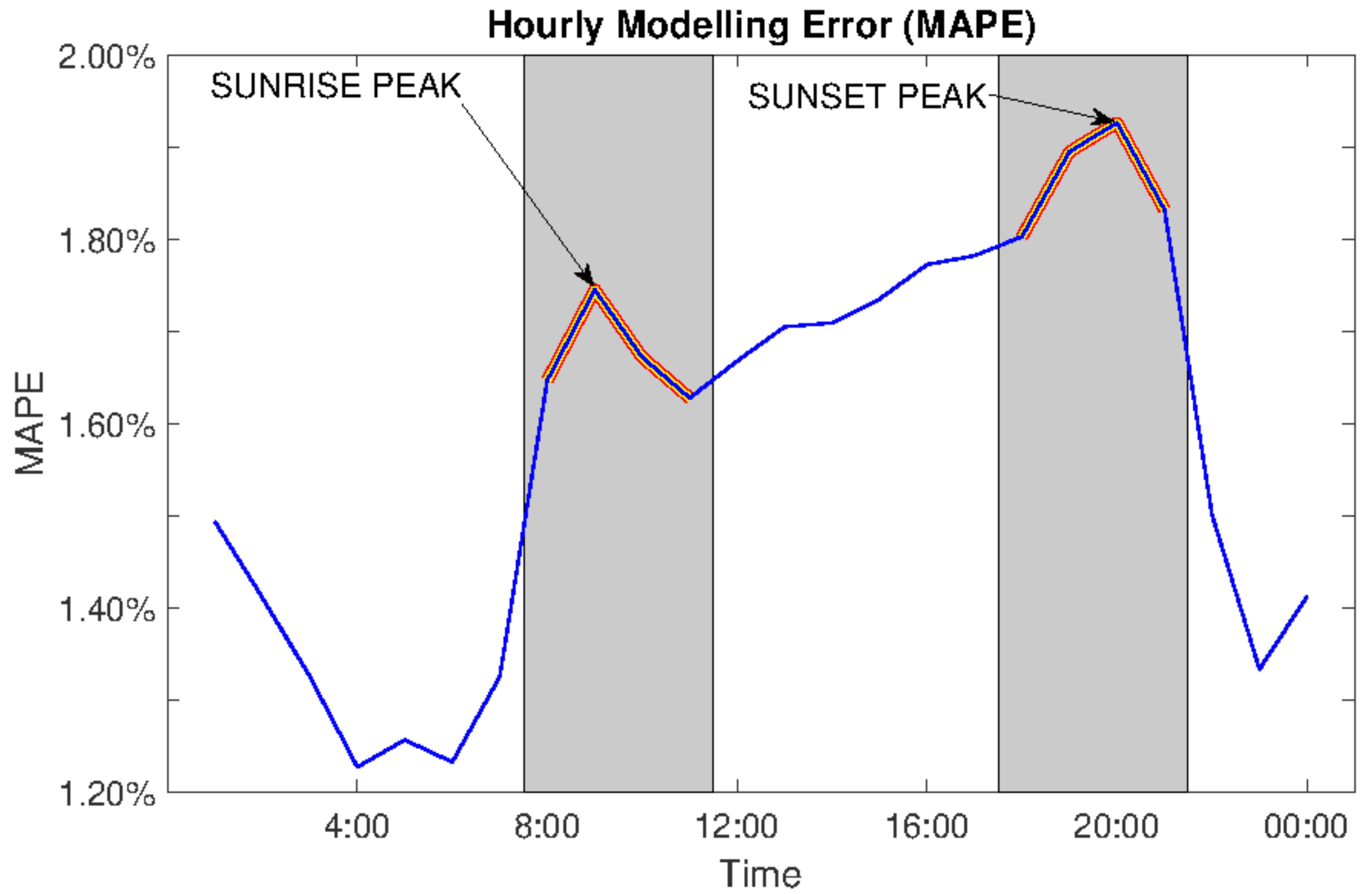
As part of the Spanish TSO’s plan to improve load forecasting, there have been several attempts to improve accuracy by using a different focus of attention: In [37], the authors analyzed the forecasting models working at REE (Red Eléctrica de España) in 2008 and compared them to two external models built by an external organization. They concluded that the existing models outperformed the challengers. In [6], a new model was proposed and this time daylight information was included in the system. The new model focused on days with extreme temperatures and holidays and special days. In [22], a first approach to including daylight information is presented but only for modeling the load, not to forecast it. More recently, in [38] another effort to improve the modeling of the non-linear effect of temperature is proposed. The results from this last research are analyzed in the results section as a benchmark. The latest analysis of the current forecasting system reveals that, as can be seen in Figure 1, the error profile has two peaks near the sunrise and sunset times. Furthermore, in the case of sunset, this error peak coincides with one of the load peaks and, therefore, its accurate forecast is especially relevant.
This paper proposes a new methodology to include available daylight into STLF models. The main contributions of this research work to the field are:
- -
- The relation between sunrise and sunset times and hourly load is modeled.
- -
- A valid linearization for this relation is presented so that it can be included in both linear or non-linear models is presented.
- -
- This new input is included in both types of models to reduce the forecasting error on sunrise and sunset times, especially when sunrise and sunset times vary faster and when DST time-shifts are implemented.
This paper is organized as follows. Section 2 describes the mathematical models tested, the data used and a detailed description and justification of the linearization proposed. It also includes a description of the different tests carried out in the design and assessment phases. In Section 3, the results of each test are detailed, to guide the reader through the design decisions and the assessment conclusions. Section 4 includes the conclusions and a recommendation to roll-out this methodology into the current forecasting system at the Spanish TSO.
2. Materials and Methods
The main objective of this paper is to reduce forecasting error on hours near sunrise and sunset times. To this end, the starting point for this research will be the forecasting model currently at use by the Spanish TSO, which was designed by our team and is thoroughly described in [6]. The most relevant characteristics of the data used by this model and its mathematical features are explained in the following section to provide a proper background to the reader. Nevertheless, the section will focus on the new additions to this model: characteristics of the daylight variables, treatment and linearization of these variables and modifications to the existing model. Further details about the input data treatment, configuration of forecasting engines, combination of output and general data flow in the original model, can be found in [6].
2.1. Model Structure
The model employs a hybrid technique in which two forecasting engines are used to provide hourly forecasts for the day in course and the next 9 days. This paper will focus on the forecast for the next day, as most papers do in order to provide a more comparable result. One of the forecasting engines uses an autoregressive neural network (NARX) while the other one uses a linear autoregressive model with errors (AR). The input analysis carried out in this paper will focus on the autoregressive (AR) model because it allows interpreting the effect of each variable. Still, the effect of the new input will be tested on both engines.
The models consider each hour of the day individually. This means that to forecast a full day, 24 models are used, each one having the same input structure. This allows for a variation of each variable’s coefficient throughout the day but causes each hour to be forecasted independently from the adjacent values.
The autoregressive part of the model significantly reduces the forecasting error by using previous errors to capture effects that are not modeled by the predictors used. This feature is beneficial in forecasting, but in modeling it may cover up the effect of the predictors—both used and missing.
In order to overcome the issues described, the AR model is modified to better suit our purposes. Firstly, the AR components are removed for the analysis of the input variables. Nevertheless, the full model with AR components will be tested at the end, once the variables are properly defined. Secondly, in order to understand how daylight affects load, it is not possible to limit each model to one hour because the variation of daylight within one hour throughout the year is too short. Therefore, the daylight variables need to be considered as global variables. The proposed model is, therefore, a linear regression with exogenous variables that affect differently each hour but also with common variables regarding daylight. It is described in (1):
where Yh is a vector with the natural logarithm of the load values at hour h each day, Xh is a matrix with the values of all exogenous variables for hour h each day, ϴh is the vector of coefficients for each variable (the same variable has a different coefficient for each hour), εh is a vector containing the residuals, Dup and Ddown are the matrices containing the piecewise variables and φup and φdown are the vectors of coefficients for the daylight variables linearization. The model described in (1) will be used to analyze the effect of the daylight variables and design their proper pre-treatment. However, once these variables have been designed, they will be introduced into the initial AR and NARX models.
2.2. Data Analysis
2.2.1. Load Data
The load data are used both as an input and as an output in the model. For this research, hourly data from the Spanish inland system from 2011 to 2018 [39] have been used. The use of large databases is important when using variables that repeat over long periods of time (temperature, daylight or holidays). Otherwise, the modeled behavior may be partial. In addition, databases may differ in predictability which increases the difficulty of comparing and analyzing accuracy results [3,40]. To avoid this issue, Table 1 includes a measure of approximate entropy (ApEn) as a measure of unpredictability. More details about this metric and its parameters can be found in [41].
Load data are used as an input in two ways:
- -
- Long-term trend: Economic growth is the main driver for long-term trends in electricity demand in Spain. The base model uses a quadratic polynomial of time to model these trends, but when larger periods of data are used for training this approach is no longer valid. In order to use more training years, the linear and quadratic terms are substituted by a 52-week moving average of the load.
- -
- Recent trend: Load series are highly autocorrelated. Therefore, even if the most relevant predictors are used, a recent value of the series has hidden information from which accuracy of the model may benefit. To this end, the base model includes the most recent known value at the time of the forecast as an input. Nevertheless, this value will not be used in the design stage of our model because it may cover up part of the effect of the variables to be analyzed.
Finally, as in most other models, the output of the model is calculated as the natural logarithm of the load.
2.2.2. Temperature Data
The temperature database that was used contains daily minimum and maximum values for the same 2011–2018 period from 59 weather stations scattered throughout the country [42]. Data series from each station are highly correlated to each other and carry very similar information. The selection of the relevant stations, linearization of the variables using the concept of heating degree days (HDD) and cooling degree days (CDD) and the determination of the lags to use is done by empiric procedure described in [6]. The results for location (Madrid-MAD, Barcelona-BCN, Seville-SEV, Zaragoza-ZAR and Bilbao-BIL) and lags used that were significant at a 0.05 level are described in Table 2:
2.2.3. Calendar Data
The type of day is a very important aspect that determines the load profile. The classification system used is very complex and it is thoroughly defined in [29]. It uses binary variables to categorize days considering the many different circumstances that affect special days in Spain.
2.2.4. Daylight
In order to include variables that represent how the consumers’ behavior is affected by available daylight at any given hour, literature suggests [43,44,45] that some hours are affected by sunset time while others are affected by sunrise. Midnight and midday hours are normally considered unaffected. In [46], sunrise and sunset time was used to quantify the effect of daylight savings time in the Spanish systems. The following paragraphs present a similar approach to include these variables in STLF models. Two raw variables are considered to capture the influence of daylight: number of hours to sunrise and number of hours to sunset, as described in (2).
where DLup and DLdown are the morning and evening variables, d is the date, h is the hour, tsunrise(d) and tsunset(d) is the sunrise and sunset times for day d in Madrid and L1 and L2 are the first and last hours of the morning interval.
The model will consider that all hours can be affected by one event, therefore all hours are assigned one variable. The threshold that splits which hours are assigned to sunrise and which are assigned to sunset will be determined empirically. In any case, it should not be a critical parameter because hours adjacent to such threshold should not be affected by either event. Sunrise and sunset times are calculated for the coordinates of Madrid.
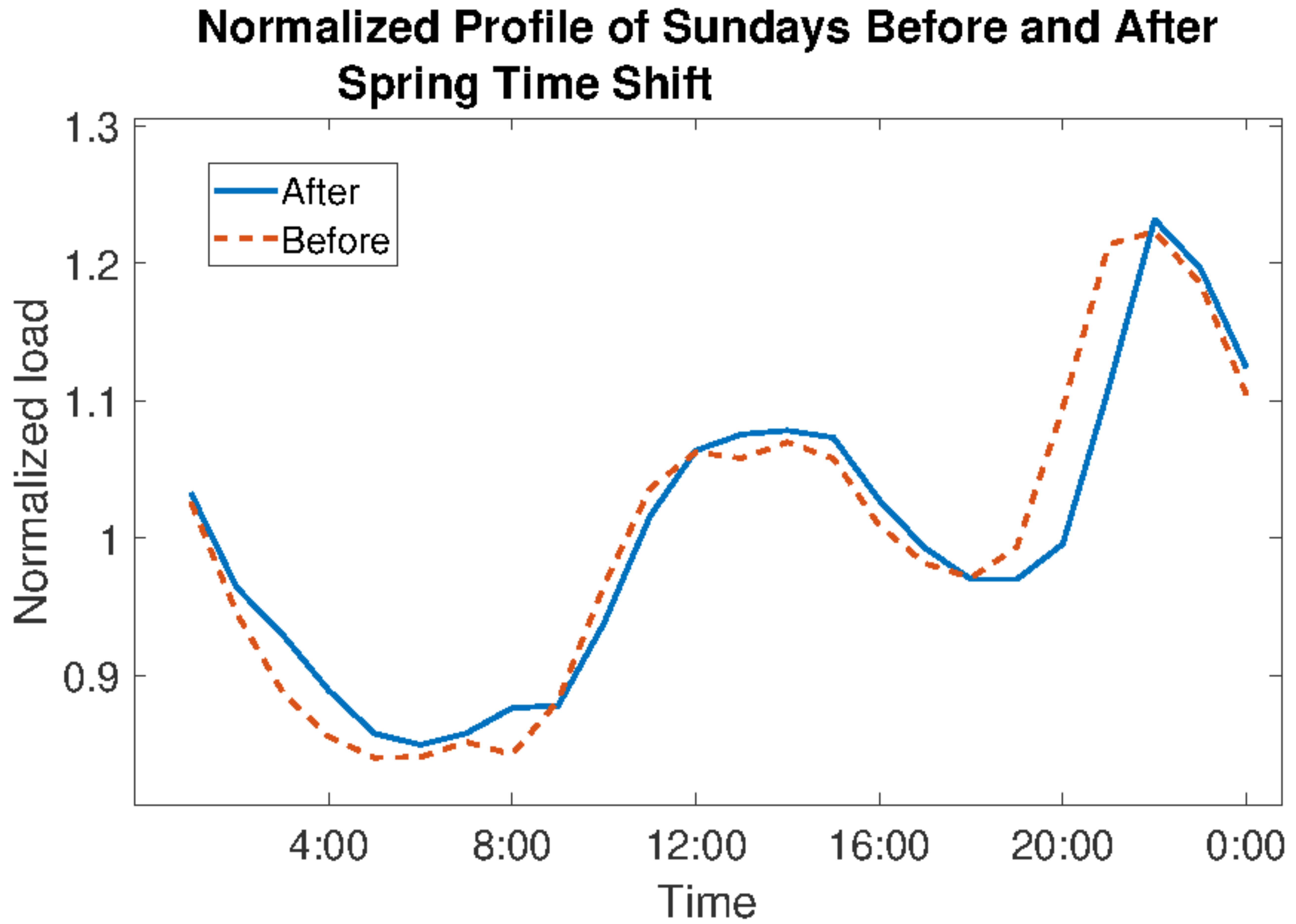
In order to understand how the daylight information should be introduced in the model, it is important to understand how it affects the load profile. The clock changes that happen when DST is set on and off are a good opportunity to visualize this. Figure 2 shows how load profile changes on a Sunday before and after the spring time shift. The evening change is much more noticeable than the morning change and midday and midnight hours seem to be unaffected. This means that the relation between load at a given hour and the number of hours to sunrise or sunset is not linear. Therefore, it is necessary to linearize the variables before entering the model.
2.3. Linearization of Daylight Variables
In order to linearize the relation between load and our daylight variables, we need to visualize the effect that they have on the load. To this end, a piecewise linearization is a good starting point to understand the relation among variables:
2.3.1. Piecewise Linearization
Piecewise linearization is used to separate each variable in intervals in which the relation between variables could be assumed to be linear and continuous among intervals. The span of sunset and sunrise intervals is separated into n intervals (INT1…n) defined by n + 1 thresholds (TH0…n). The number of intervals is set empirically to an interval length of 60 min after testing 15-, 30-, 60- and 120-min long intervals. Longer intervals caused larger fitting errors while shorter intervals provoked overfitting.
The linearization is realized by creating two new variables (slope and intercept) for each interval. Both initial variables DLup and DLdown are linearized so a total of 2 × n × 2 = 4n variables are created. These variables are described in (3):
where Mup/dw,i Kup/dw,i are the slope and intercepts variables for the ith interval for either the morning or evening function, respectively, and DLup/dw(d,h) is either the morning or evening function.
These 2 times 2n variables provide a slope and an intercept for each of the intervals defined. However, this does not imply continuity of the response. In order to force continuity in the domain of the variables, it is necessary to introduce a series of restrictions forcing each adjacent interval to have the same value at the shared threshold. These restrictions are described in (4):
where mi and ki are the slope and intercept coefficients for the ith interval.
These restrictions reduce the number of variables because they restrict the value of the coefficient. Each restriction subtracts one variable, so the new number of variables is 2 × (2n − (n − 1)) = 2 (n +1). These new variables are described in (5):
where Vup/dw,i(d,h) is the ith variable of either the sunrise or sunset group. Each variable takes a value of zero if the hour h does not belong to the corresponding group.
The model described in (1) allows us to interpret the effect that the daylight variables have on electricity consumption. By isolating the part of the model that deals with daylight variables it is possible to obtain the corresponding coefficient for each instant. These coefficients are the response of the load to variations in available daylight and they are described in (6):
2.3.2. Sigmoid Linearization
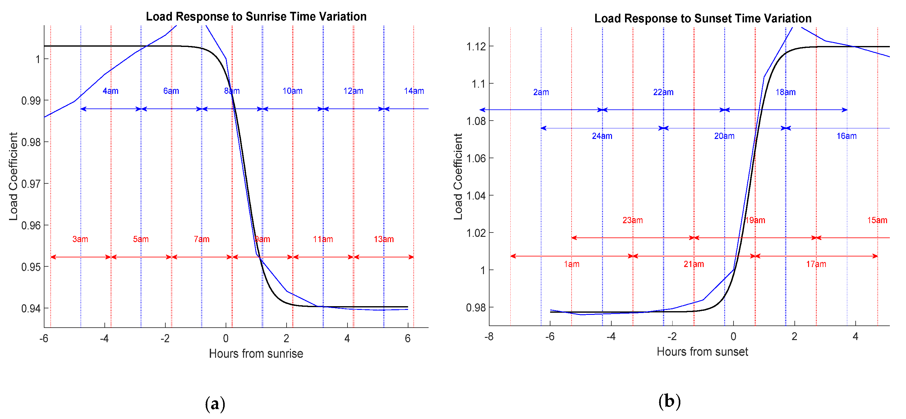
The curves seen in Figure 3 show a stable coefficient for hours far before sunrise or sunset; there is a steep change around each event and again a constant coefficient for hours long after. This behavior can be approximated by the sigmoid function described in (7):
where b, L, k and DL0 are the parameters that determine the size of the step, its position on both axes and the slope in the transition. These parameters have different values for the sunrise and sunset linearizations and can be obtained from fitting the sigmoid response to the piecewise response. The results are shown in (8):
where Rt(−∞) is the natural logarithm of the average value of the right side of the curve, Rt(∞) is the natural logarithm of the average value of the left side and R’t represents the slope.
Figure 3 shows the comparison of both linearizations. The curves include the intervals in which each hour may vary throughout the year. Due to the current DST policy, the time to sunrise for any hour varies only two hours from winter to summer while the time to sunset varies four hours throughout the year.
2.3.3. Validation of Linearized Variables
Both linearizations show a similar behavior but the sigmoid linearization requires less variables. In order to assess the quality of each linearization, the modeling error of each model will be compared. As a base reference, a third model without any information regarding daylight will also be tested.
The test consists on an out-of-sample test using data from 2011 to 2017 in which data from every other year is used to model each year. The results are shown in Table 3. Other modeling and forecasting errors from the same database can be found in [6,37] for context.
The results show that both linearizations provide a very similar result and that, as expected, their use drastically reduces the modeling error at sunrise and sunset hours. Considering that the sigmoid linearization matches the piecewise accuracy with a fraction of the variables, the sigmoid linearization is chosen.
2.3.4. Other Modeling Improvements
The variations in load as available daylight changes is due to consumers’ behavior. Still, it is arguable that their behavior will change in the same way, regardless of the day of the week. In order to allow for this variation for different types of days, the model includes a different set of daylight variables as described in (7) for each type of day. The categories considered after testing other combinations are Mondays, Sundays and holidays, Saturdays, and the rest of the weekdays.
2.4. Description of Tests
As it was aforementioned, the aim of the paper is to provide a methodology that improves forecasting accuracy through the use of available daylight information. In order to assess the different possibilities considered, several changes have been made from the original forecasting model in the design and testing stages.
The metric used to compare results is the mean average percentage error (MAPE) as described in (9). The simulation conditions are day-ahead predictions cast at 10 a.m. the day before. For the design phase, the data used is from 2011 to 2017, and the model used corresponds to the AR model stripped from its autoregressive components as described in (1). In order to obtain out-of-sample results, each year is simulated using a model estimated with the rest of the years. In that way, we obtain a 7-year-long period of results. The design phase allows us to determine the best model, which is then tested in the assessment phase.
where MAPEd is the MAPE for day d, Fd,h is the forecast for day d at hour h and Ld,h is the actual load on day d and hour h.
In the assessment phase, both the AR and neural network (NN) models are used, including all of their designed features. The testing data is a 1-year-long period of 2018, and the model is estimated with the previous data (2011–2017).
3. Results
This section presents the results not only for the final model but also for the design phase, as a justification of the design decisions and a guide to the application of this methodology to other databases. The benchmark used to compare the results of the model is the current forecast used by the system TSO, as our proposed model is held to the same computational restrictions and deals with the same database. Comparison across techniques applied to different databases may hide differences in the predictability of each data series and may lead to wrong conclusions about the quality of each technique [3]. The computational burden of the proposed model is the same as that of the previous system.
3.1. Design Results
Six different input configurations were tested in this stage. The details of each configuration are included in Table 4.
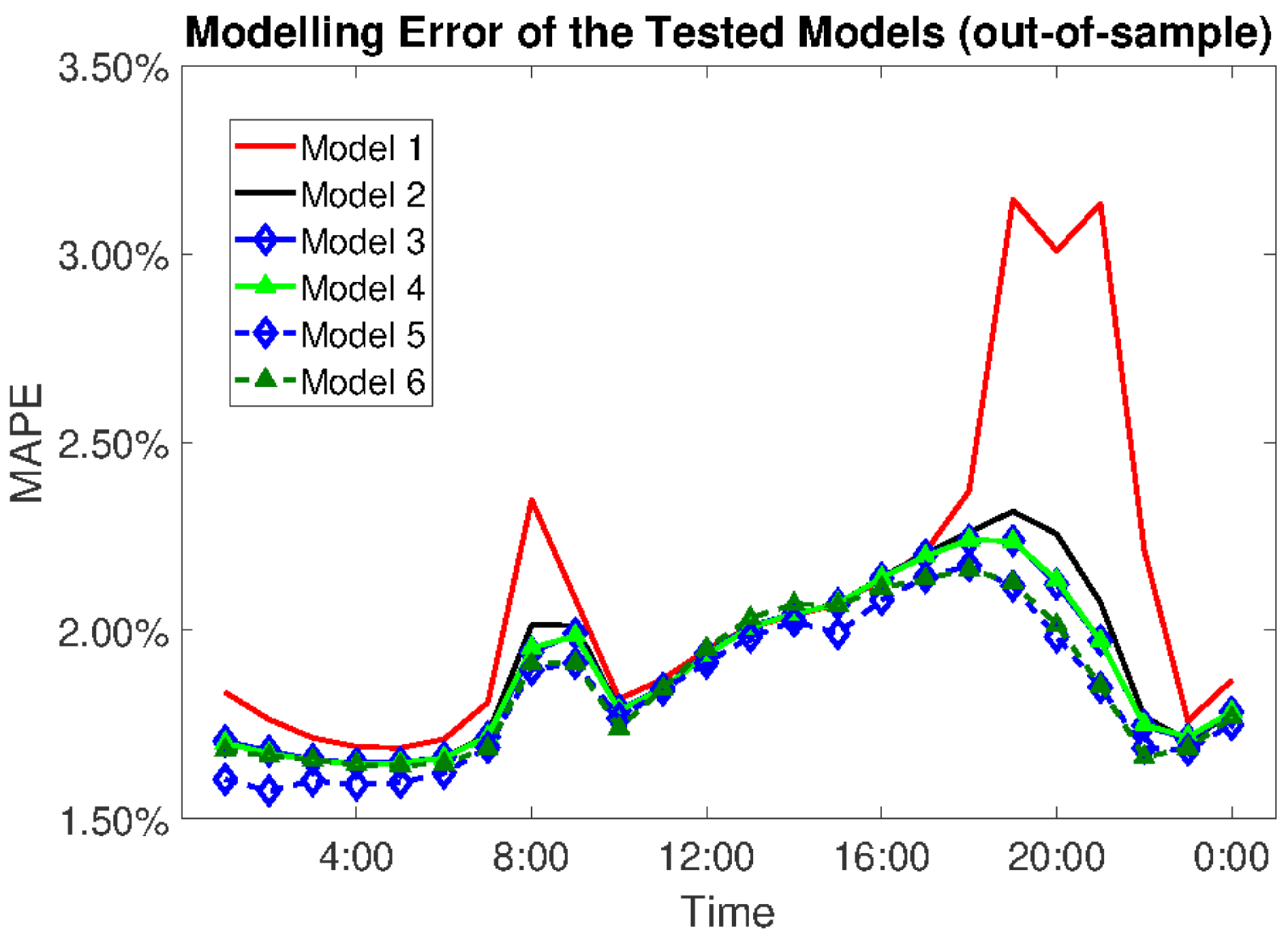
The results for the out-of-sample tests are shown in Figure 4. Table 5 also shows the results by grouping the different periods: sunrise, sunset, mid-day and mid-night.
The results allow drawing similar conclusions:
- -
- Midday and midnight hours are not improved significantly by the addition of available daylight information other than the month information. Midday and midnight modeling errors vary in a range of barely 0.07 percentage points.
- -
- Sunrise hours are improved from 1.92% to 1.83%.
- -
- Sunset hours are more significantly improved, going from 2.14% to 1.96% in out-of-sample test.
From Figure 4 it can be seen that in the sunrise and sunset intervals both linearizations (traces 3 and 4) are essentially equivalent and that the first improvement comes from using either one of them and then, a second increase in accuracy is obtained by discriminating by type of day.
Considering that the model 5 uses 35 more variables than model 6, the piecewise linearization is discarded for the assessment phase and the type of day discrimination is found to be significant.
3.2. Assessment Results
The previous section presented the results that led to the selection of a sigmoid linearization with type-of-day discrimination due to its accuracy and low number of variables used. The errors presented were out-of-sample modeling errors. Nonetheless, the actual assessment of this paper’s contribution is to compare the original forecasting model used by the TSO with the proposed one in real conditions. To this end, the AR model is restored to its original configuration and the new variables are added as input. The two configurations are compared using new data from 2018.
Table 6 presents the forecasting errors of both models along with the forecasting error of the NN model also used in the TSO’s ensemble. This NN model does not include any information regarding daylight other than what was already included in the original model. Table 6 also includes the results of the week after DST is implemented. This particular week is especially sensitive to the modeled phenomenon and, therefore it is a good reference value:
The results show that the inclusion of available daylight information causes a reduction of the forecasting error in sunrise and sunset times of 0.12 and 0.18 percentage points respectively. As expected, midday and midnight hours remain unaffected. This accuracy improvement turns the AR model into the best performing model during sunset hours. The overall result indicates that the new AR model is nearly as accurate as the NN model. All these conclusions are even more obvious from the DST week results.
Proposed Model vs. NN
The new variables have been introduced in the AR model in order to obtain a significant improvement on sunrise and sunset hours. Table 6 includes results from the original NN model as a comparison for both AR models. However, the question of whether the NN can be improved remains.
Several attempts to include available daylight information into the NN model were carried out. Considering the NN inherent ability to model non-linear behavior, the original variables of the number of hours to sunrise and sunset were included. Also, on a separate attempt, the linearized variables were also tested, yet, none of these tests yielded any improvement in accuracy of the NN model.
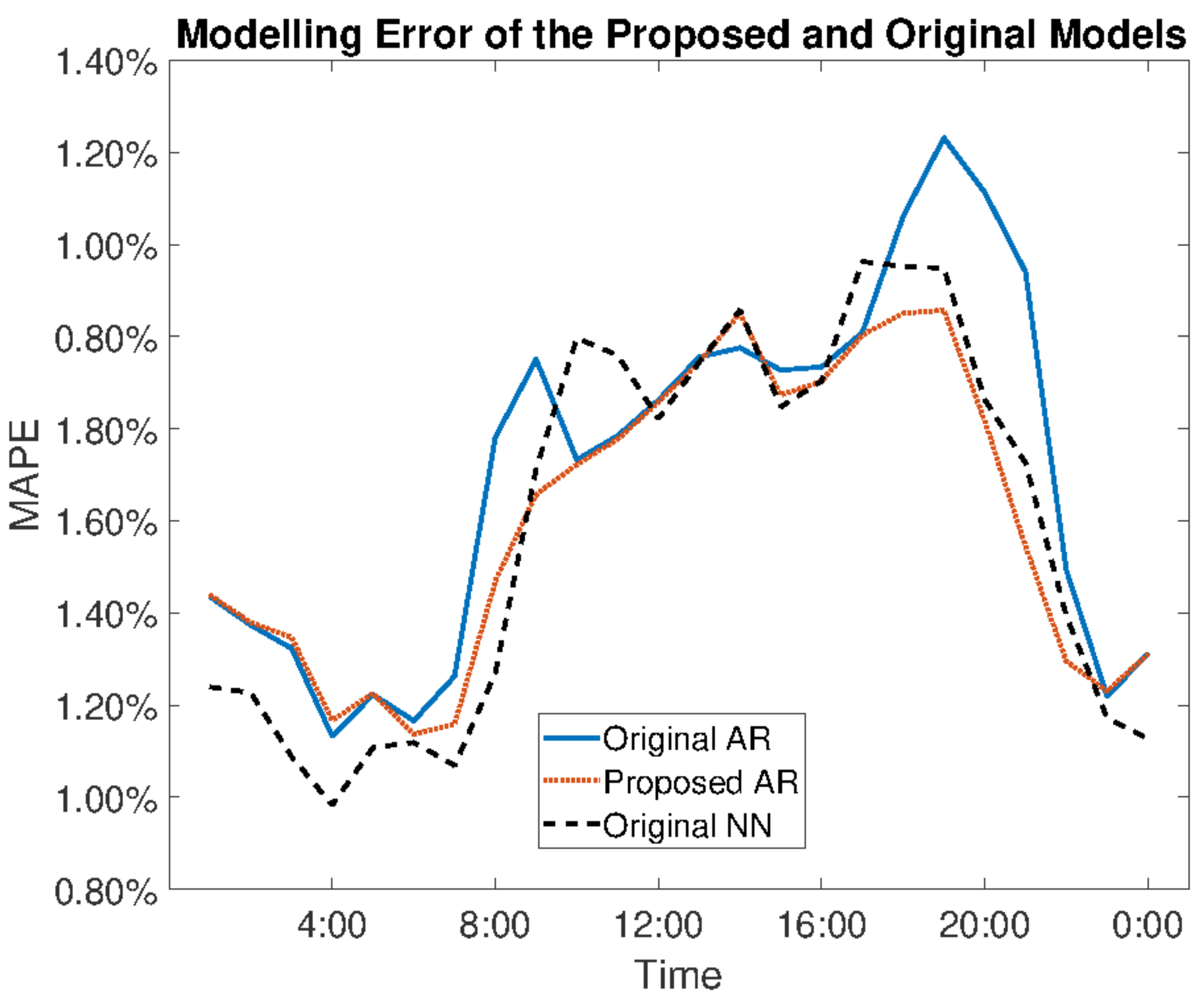
Figure 5 shows the NN model’s result on 2018 compared to the AR models. It shows how the NN model does not show the sunrise and sunset error humps that this paper addresses. This behavior could be explained through the non-linear behavior of the NN model and the high correlation between temperature (already in the model) and daylight. The fact that the AR model became so much more similar to the NN model when the available daylight information was introduced that it leads to thinking that while the NN was able to model this behavior from its original variables, the AR model needed the linearization provided to increase its accuracy.
The final forecast emitted by the system is a linear combination of both the AR and NN models. Table 7 shows how the weight in the combination has shifted towards the AR model and the final improvement of the overall system. Such combination is the result of an algorithm implemented to minimize error based on the last 30 days. Further details of this process can be found in [6].
The results of Table 7 include other references as context for the provided results. All the references used refer to the same electric system because comparing accuracy using different databases can be misleading, as some systems are more predictable than others. Nevertheless, the proposed model presents a clear advantage during sunrise and sunset hours over all reported results.
All these results were obtained on an i7 2.2GHz PC with 16Gb of RAM under real-time conditions. A ten-day forecast is emitted every hour with a computing time of 5.3 min on average that includes reading input files, processing the forecast and writing output files.
4. Conclusions
The possible inputs for STLF models include previous loads, calendar variables, and environmental variables like temperature, humidity or daylight. However, even though the use of electric lighting depends directly on available daylight, its use is scarce in the literature as its own variable.
This paper proposes a methodology for including available daylight information into STLF models to achieve the goal of reducing forecasting error during sunrise and sunset hours. It uses as raw variables the number of hours until sunrise and sunset, it describes how sunrise and sunset hours are affected differently and how the non-linear relation between load and the raw variables should be linearized through sigmoid functions without over-complicating the model.
The methodology has been tested using out-of-sample data from 2018. The full-year results are compared with other models currently running at the National Transmission System Operator in Spain, proving that the followed approach leads to significant increase in short-term load forecasting accuracy, especially focused on sunrise (1.33% to 1.21%) and sunset (1.56% to 1.38%). The improvement is even more relevant on the weeks in which DST is implemented and daylight changes suddenly: sunrise error falls from 1.90% to 1.37% and sunset error drops from 2.53% to 2.09%. The inclusion of this variables did not cause any improvements in the forecasting model based on neural networks. However, the linear combination of both models used reflected the sunrise and sunset improvement (1.09% vs. 1.12% and 1.30% vs. 1.37%, respectively) and increased the weight of the new AR model (from 37% to 59%).
The methodology described in this paper will be rolled out into the TSO’s forecasting system in 2020 as it will help reduce forecasting error especially at peak hours like sunset, in which inaccuracies are particularly costly to the system.
Author Contributions
Conceptualization, M.L.; methodology, M.L.; software, M.L.; and C.S. (Carlos Sans); validation, C.S. (Carlos Sans), C.S. (Carolina Senabre); formal analysis, M.L.; investigation, M.L.; resources, C.S. (Carlos Sans); data curation, C.S. (Carolina Senabre); writing—original draft preparation, M.L.; writing—review and editing, C.S. (Carolina Senabre); supervision, S.V.; project administration, S.V.; funding acquisition, S.V. All authors have read and agreed to the published version of the manuscript.
Funding
This research received no external funding.
Institutional Review Board Statement
Not applicable.
Informed Consent Statement
Not applicable.
Data Availability Statement
Restrictions apply to the availability of these data. Data was obtained from REE and AEMET and are available at https://www.esios.ree.es/es and http://www.aemet.es/es/datos_abiertos.
Acknowledgments
This research is a byproduct of a collaboration project between Red Eléctrica de España and Universidad Miguel Hernández. Open access costs will be funded by this project.
Conflicts of Interest
The authors declare no conflict of interest. The funding sponsors had no role in the design of the study; in the collection, analyses, or interpretation of data; in the writing of the manuscript, and in the decision to publish the results.
References
- Chamandoust, H.; Derakhshan, G.; Hakimi, S.M.; Bahramara, S. Tri-Objective Optimal Scheduling of Smart Energy Hub System with Schedulable Loads. J. Clean. Prod. 2019, 236, 117584. [Google Scholar] [CrossRef]
- Hippert, H.S.; Pedreira, C.E.; Souza, R.C. Neural Networks for Short-Term Load Forecasting: A Review and Evaluation. IEEE Trans. Power Syst. 2001, 16, 44–55. [Google Scholar] [CrossRef]
- Lopez Garcia, M.; Valero, S.; Senabre, C.; Gabaldon Marin, A. Short-Term Predictability of Load Series: Characterization of Load Data Bases. IEEE Trans. Power Syst. 2013, 28, 2466–2474. [Google Scholar] [CrossRef]
- Hernandez, L.; Baladron, C.; Aguiar, J.M.; Carro, B.; Sanchez-Esguevillas, A.J.; Lloret, J.; Massana, J. A Survey on Electric Power Demand Forecasting: Future Trends in Smart Grids, Microgrids and Smart Buildings. IEEE Commun. Surv. Tutor. 2014, 16, 1460–1495. [Google Scholar] [CrossRef]
- Kuster, C.; Rezgui, Y.; Mourshed, M. Electrical Load Forecasting Models: A Critical Systematic Review. Sustain. Cities Soc. 2017, 35, 257–270. [Google Scholar] [CrossRef]
- López, M.; Valero, S.; Rodriguez, A.; Veiras, I.; Senabre, C. New Online Load Forecasting System for the Spanish Transport System Operator. Electr. Power Syst. Res. 2018, 154, 401–412. [Google Scholar] [CrossRef]
- Charlton, N.; Singleton, C. A Refined Parametric Model for Short Term Load Forecasting. Int. J. Forecast. 2014, 30, 364–368. [Google Scholar] [CrossRef] [Green Version]
- Wang, P.; Liu, B.; Hong, T. Electric Load Forecasting with Recency Effect: A Big Data Approach. Int. J. Forecast. 2016, 32, 585–597. [Google Scholar] [CrossRef] [Green Version]
- Yun, Z.; Quan, Z.; Caixin, S.; Shaolan, L.; Yuming, L.; Yang, S. RBF Neural Network and ANFIS-Based Short-Term Load Forecasting Approach in Real-Time Price Environment. IEEE Trans. Power Syst. 2008, 23, 853–858. [Google Scholar] [CrossRef]
- López, M.; Valero, S.; Senabre, C.; Aparicio, J.; Gabaldon, A. Application of SOM Neural Networks to Short-Term Load Forecasting: The Spanish Electricity Market Case Study. Electr. Power Syst. Res. 2012, 91, 18–27. [Google Scholar] [CrossRef]
- Hinojosa, V.H.; Hoese, A. Short-Term Load Forecasting Using Fuzzy Inductive Reasoning and Evolutionary Algorithms. IEEE Trans. Power Syst. 2010, 25, 565–574. [Google Scholar] [CrossRef]
- Wang, J.; Jin, S.; Qin, S.; Jiang, H. Swarm Intelligence-Based Hybrid Models for Short-Term Power Load Prediction. Math. Probl. Eng. 2014, 2014, 17. [Google Scholar] [CrossRef] [Green Version]
- Bashir, Z.A.; El-Hawary, M.E. Applying Wavelets to Short-Term Load Forecasting Using PSO-Based Neural Networks. IEEE Trans. Power Syst. 2009, 24, 20–27. [Google Scholar] [CrossRef]
- Amjady, N.; Keynia, F. Short-Term Load Forecasting of Power Systems by Combination of Wavelet Transform and Neuro-Evolutionary Algorithm. Energy 2009, 34, 46–57. [Google Scholar] [CrossRef]
- Ghadimi, N.; Akbarimajd, A.; Shayeghi, H.; Abedinia, O. Two Stage Forecast Engine with Feature Selection Technique and Improved Meta-Heuristic Algorithm for Electricity Load Forecasting. Energy 2018, 161, 130–142. [Google Scholar] [CrossRef]
- Gao, W.; Darvishan, A.; Toghani, M.; Mohammadi, M.; Abedinia, O.; Ghadimi, N. Different States of Multi-Block Based Forecast Engine for Price and Load Prediction. Int. J. Electr. Power Energy Syst. 2019, 104, 423–435. [Google Scholar] [CrossRef]
- Motepe, S.; Hasan, A.N.; Stopforth, R. Improving Load Forecasting Process for a Power Distribution Network Using Hybrid AI and Deep Learning Algorithms. IEEE Access 2019, 7, 82584–82598. [Google Scholar] [CrossRef]
- Ryu, S.; Noh, J.; Kim, H. Deep Neural Network Based Demand Side Short Term Load Forecasting. Energies 2016, 10, 3. [Google Scholar] [CrossRef]
- Yin, L.; Sun, Z.; Gao, F.; Liu, H. Deep Forest Regression for Short-Term Load Forecasting of Power Systems. IEEE Access 2020, 8, 49090–49099. [Google Scholar] [CrossRef]
- Kong, W.; Dong, Z.Y.; Jia, Y.; Hill, D.J.; Xu, Y.; Zhang, Y. Short-Term Residential Load Forecasting Based on LSTM Recurrent Neural Network. IEEE Trans. Smart Grid 2019, 10, 841–851. [Google Scholar] [CrossRef]
- Chen, K.; Chen, K.; Wang, Q.; He, Z.; Hu, J.; He, J. Short-Term Load Forecasting With Deep Residual Networks. IEEE Trans. Smart Grid 2019, 10, 3943–3952. [Google Scholar] [CrossRef] [Green Version]
- Moral-Carcedo, J.; Pérez-García, J. Time of Day Effects of Temperature and Daylight on Short Term Electricity Load. Energy 2019, 174, 169–183. [Google Scholar] [CrossRef]
- Zhang, N.; Li, Z.; Zou, X.; Quiring, S.M. Comparison of Three Short-Term Load Forecast Models in Southern California. Energy 2019, 189, 116358. [Google Scholar] [CrossRef]
- Haben, S.; Giasemidis, G.; Ziel, F.; Arora, S. Short Term Load Forecasting and the Effect of Temperature at the Low Voltage Level. Int. J. Forecast. 2019, 35, 1469–1484. [Google Scholar] [CrossRef] [Green Version]
- Wang, Y.; Bielicki, J.M. Acclimation and the Response of Hourly Electricity Loads to Meteorological Variables. Energy 2018, 142, 473–485. [Google Scholar] [CrossRef]
- López, M.; Valero, S.; Senabre, C.; Gabaldón, A. Analysis of the Influence of Meteorological Variables on Real-Time Short-Term Load Forecasting in Balearic Islands. In Proceedings of the 2017 11th IEEE International Conference on Compatibility, Power Electronics and Power Engineering (CPE-POWERENG), Cadiz, Spain, 1 May 2017; pp. 10–15. [Google Scholar]
- Fan, S.; Chen, L. Short-Term Load Forecasting Based on an Adaptive Hybrid Method. IEEE Trans. Power Syst. 2006, 21, 392–401. [Google Scholar] [CrossRef]
- Arora, S.; Taylor, J.W. Short-Term Forecasting of Anomalous Load Using Rule-Based Triple Seasonal Methods. IEEE Trans. Power Syst. 2013, 28, 3235–3242. [Google Scholar] [CrossRef] [Green Version]
- López, M.; Sans, C.; Valero, S.; Senabre, C. Classification of Special Days in Short-Term Load Forecasting: The Spanish Case Study. Energies 2019, 12, 1253. [Google Scholar] [CrossRef] [Green Version]
- Rivers, N. Does Daylight Savings Time Save Energy? Evidence from Ontario. Environ. Resour. Econ. 2017. [Google Scholar] [CrossRef]
- Choi, S.; Pellen, A.; Masson, V. How Does Daylight Saving Time Affect Electricity Demand? An Answer Using Aggregate Data from a Natural Experiment in Western Australia. Energy Econ. 2017, 66, 247–260. [Google Scholar] [CrossRef]
- Verdejo, H.; Becker, C.; Echiburu, D.; Escudero, W.; Fucks, E. Impact of Daylight Saving Time on the Chilean Residential Consumption. Energy Policy 2016, 88, 456–464. [Google Scholar] [CrossRef]
- Hill, S.I.; Desobry, F.; Garnsey, E.W.; Chong, Y.-F. The Impact on Energy Consumption of Daylight Saving Clock Changes. Energy Policy 2010, 38, 4955–4965. [Google Scholar] [CrossRef]
- Afshin, M.; Sadeghian, A. PCA-Based Least Squares Support Vector Machines in Week-Ahead Load Forecasting. In Proceedings of the 2007 IEEE/IAS Industrial & Commercial Power Systems Technical Conference, Edmonton, AB, Canada, 6–11 May 2007; pp. 1–6. [Google Scholar]
- Bessec, M.; Fouquau, J. Short-Run Electricity Load Forecasting with Combinations of Stationary Wavelet Transforms. Eur. J. Oper. Res. 2018, 264, 149–164. [Google Scholar] [CrossRef]
- Do, L.P.C.; Lin, K.-H.; Molnár, P. Electricity Consumption Modelling: A Case of Germany. Econ. Model. 2016, 55, 92–101. [Google Scholar] [CrossRef]
- Cancelo, J.R.; Espasa, A.; Grafe, R. Forecasting the Electricity Load from One Day to One Week Ahead for the Spanish System Operator. Int. J. Forecast. 2008, 24, 588–602. [Google Scholar] [CrossRef] [Green Version]
- Caro, E.; Juan, J.; Cara, J. Periodically Correlated Models for Short-Term Electricity Load Forecasting. Appl. Math. Comput. 2020, 364, 124642. [Google Scholar] [CrossRef]
- ESIOS REE-Information System for the Electric System Operator. Available online: https://www.esios.ree.es/es2019 (accessed on 7 July 2019).
- Peng, Y.; Wang, Y.; Lu, X.; Li, H.; Shi, D.; Wang, Z.; Li, J. Short-Term Load Forecasting at Different Aggregation Levels with Predictability Analysis. In Proceedings of the 2019 IEEE Innovative Smart Grid Technologies-Asia (ISGT Asia), Chengdu, China, 21–24 May 2019; pp. 3385–3390. [Google Scholar]
- Pincus, S.M. Approximate Entropy: A Complexity Measure for Biological Time Series Data. In Proceedings of the Proceedings of the 1991 IEEE Seventeenth Annual Northeast Bioengineering Conference, Hartford, CT, USA, 4–5 April 1991; pp. 35–36. [Google Scholar]
- AEMET OpenData. 2019. Available online: http://www.aemet.es/es/datos_abiertos (accessed on 15 July 2019).
- Kotchen, M.J.; Grant, L.E. Does Daylight Saving Time Save Energy? Evidence from a Natural Experiment in Indiana. Rev. Econ. Stat. 2011, 93, 1172–1185. [Google Scholar] [CrossRef] [Green Version]
- Kellogg, R.; Wolff, H. Daylight Time and Energy: Evidence from an Australian Experiment. J. Environ. Econ. Manag. 2008, 56, 207–220. [Google Scholar] [CrossRef]
- Mirza, F.M.; Bergland, O. The Impact of Daylight Saving Time on Electricity Consumption: Evidence from Southern Norway and Sweden. Energy Policy 2011, 39, 3558–3571. [Google Scholar] [CrossRef]
- López, M. Daylight Effect on the Electricity Demand in Spain and Assessment of Daylight Saving Time Policies. Energy Policy 2020, 140, 111419. [Google Scholar] [CrossRef]
Figure 1.
Average hourly error of the autoregressive model currently running at REE headquarters. The figure shows two humps from 7 a.m. to 10 a.m. and from 6 p.m. to 10 p.m.
Figure 1.
Average hourly error of the autoregressive model currently running at REE headquarters. The figure shows two humps from 7 a.m. to 10 a.m. and from 6 p.m. to 10 p.m.

Figure 2.
Normalized profiles of the Sunday before and after the daylight savings time (DST) time shift in March.
Figure 2.
Normalized profiles of the Sunday before and after the daylight savings time (DST) time shift in March.

Figure 3.
Response to daylight as a coefficient for the expected load. Both piece-wise and sigmoidal linearizations are represented to show a good fit between them. (a) sunrise and (b) sunset.
Figure 3.
Response to daylight as a coefficient for the expected load. Both piece-wise and sigmoidal linearizations are represented to show a good fit between them. (a) sunrise and (b) sunset.

Figure 4.
Average modeling error by time of day with out-of-sample testing.

Figure 5.
Forecasting error by time of day of the original and proposed autoregressive (AR) models and the neural network (NN) model.
Figure 5.
Forecasting error by time of day of the original and proposed autoregressive (AR) models and the neural network (NN) model.


Table 1.
Approximate entropy.
| Embedded Dimension | 1 | 4 | 8 | 12 | 16 | 20 | 24 |
|---|---|---|---|---|---|---|---|
| ApEn | 1.038 | 0.553 | 0.266 | 0.125 | 0.078 | 0.058 | 0.034 |
| Time delay = 1; radius = 0.2 times the standard deviation of the load series | |||||||
Table 2.
Temperature variables significant at a 0.05 level.
| Lag | MAD | BCN | SEV | ZAR | BIL |
|---|---|---|---|---|---|
| 0 | HDD/CDD | HDD/CDD | HDD/CDD | HDD/CDD | ---/CDD |
| 1 | ---/--- | HDD/CDD | ---/--- | ---/--- | ---/--- |
| 2 | ---/--- | ---/--- | ---/--- | ---/--- | ---/--- |
Table 3.
Modeling error for each time of day for out-of-sample tests.
| Out-of-Sample | 7 a.m. | 8 a.m. | 9 a.m. | Avg. Sunrise | 4 p.m. | 5 p.m. | 6 p.m. | 7 p.m. | 8 p.m. | 9 p.m. | 10 p.m. | Avg. Sunset | Avg. Rest |
|---|---|---|---|---|---|---|---|---|---|---|---|---|---|
| w/o daylight | 2.23% | 2.91% | 2.76% | 2.63% | 2.47% | 2.50% | 2.68% | 3.65% | 3.61% | 3.55% | 2.51% | 2.86% | 2.30% |
| piecewise | 2.21% | 2.52% | 2.62% | 2.45% | 2.47% | 2.49% | 2.50% | 2.44% | 2.37% | 2.24% | 2.09% | 2.40% | 2.30% |
| sigmoid | 2.21% | 2.55% | 2.61% | 2.46% | 2.47% | 2.50% | 2.51% | 2.43% | 2.35% | 2.24% | 2.08% | 2.40% | 2.30% |
Table 4.
Description of the models tested in the design phase.
| # | Name | Description | Vars. Per Hour | Period |
|---|---|---|---|---|
| 1 | Base w/o month | Original model in which eleven binary variables coding the month are removed. | 87 | 2011–2017 |
| 2 | Base | Original model | 98 | |
| 3 | Base + piecewise | Original model with piecewise linearization (n = 10) | 108 | |
| 4 | Base + sigmoid | Original model with sigmoid linearization | 99 | |
| 5 | Base + piecewise by type of day | Original model with piecewise linearization for each type of day (n = 10). | 138 | |
| 6 | Base + sigmoid by type of day | Original model with sigmoid linearization for each type of day. | 103 |
Table 5.
Modeling error for each time of day for 2018.
| Model Nr. | Sunrise (7 a.m.–9 a.m.) | Mid-Day (10 a.m.–5 p.m.) | Sunset (6 p.m.–10 p.m.) | Mid-Night (11 p.m.–6 a.m.) | All Day |
|---|---|---|---|---|---|
| 1 | 2.08% | 2.01% | 2.77% | 1.81% | 2.09% |
| 2 | 1.92% | 2.00% | 2.14% | 1.72% | 1.91% |
| 3 | 1.88% | 2.00% | 2.06% | 1.72% | 1.90% |
| 4 | 1.89% | 2.00% | 2.07% | 1.72% | 1.90% |
| 5 | 1.83% | 1.97% | 1.96% | 1.65% | 1.84% |
| 6 | 1.84% | 1.99% | 1.96% | 1.70% | 1.86% |
Table 6.
Forecasting error for each time of day for 2018.
| Model | Sunrise (7 a.m.–9 a.m.) | Mid-Day | Sunset (6 p.m.–10 p.m.) | Mid-Night | All Day | |
|---|---|---|---|---|---|---|
| OVERALL | Original AR | 1.33% | 1.45% | 1.56% | 1.17% | 1.35% |
| Proposed AR | 1.21% | 1.45% | 1.38% | 1.17% | 1.30% | |
| Original NN | 1.18% | 1.48% | 1.43% | 1.10% | 1.29% | |
| DST WEEK | Original AR | 1.90% | 1.85% | 2.53% | 1.44% | 1.85% |
| Proposed AR | 1.37% | 1.80% | 2.09% | 1.42% | 1.67% | |
| Original NN[M1] | 1.35% | 1.83% | 2.14% | 1.38% | 1.68% |
Table 7.
Forecasting error of the benchmark and AR and NN models combined.
| Model | Sunrise (7 a.m.–9 a.m.) | Mid-Day | Sunset (6 p.m.–10 p.m.) | Mid-Night | All Day |
|---|---|---|---|---|---|
| Persistent (7-days) | 4.64% | 5.10% | 5.18% | 3.68% | 4.58% |
| * Cancelo et Al [37] | 1.48% | 1.67% | 1.70% | 1.38% | 1.56% |
| Original AR 37% + NN 63% | 1.12% | 1.36% | 1.37% | 1.04% | 1.21% |
| * Caro et Al [38] | 1.26% | 1.33% | 1.44% | 1.06% | 1.25% |
| Proposed AR 59% + NN 41% | 1.09% | 1.34% | 1.30% | 1.05% | 1.20% |
* Results refer to a forecast of data from 2006.
Publisher’s Note: MDPI stays neutral with regard to jurisdictional claims in published maps and institutional affiliations. |
© 2020 by the authors. Licensee MDPI, Basel, Switzerland. This article is an open access article distributed under the terms and conditions of the Creative Commons Attribution (CC BY) license (http://creativecommons.org/licenses/by/4.0/).
Share and Cite
MDPI and ACS Style
López, M.; Valero, S.; Sans, C.; Senabre, C. Use of Available Daylight to Improve Short-Term Load Forecasting Accuracy. Energies 2021, 14, 95. https://0-doi-org.brum.beds.ac.uk/10.3390/en14010095
AMA Style
López M, Valero S, Sans C, Senabre C. Use of Available Daylight to Improve Short-Term Load Forecasting Accuracy. Energies. 2021; 14(1):95. https://0-doi-org.brum.beds.ac.uk/10.3390/en14010095
Chicago/Turabian StyleLópez, Miguel, Sergio Valero, Carlos Sans, and Carolina Senabre. 2021. "Use of Available Daylight to Improve Short-Term Load Forecasting Accuracy" Energies 14, no. 1: 95. https://0-doi-org.brum.beds.ac.uk/10.3390/en14010095
Note that from the first issue of 2016, this journal uses article numbers instead of page numbers. See further details here.