Deep Convolutional Feature-Based Probabilistic SVDD Method for Monitoring Incipient Faults of Batch Process

Abstract

Support vector data description (SVDD) has been widely applied to batch process fault detection. However, it often performs poorly, especially when incipient faults occur, because it only considers the shallow data feature and omits the probabilistic information of features. In order to provide better monitoring performance on incipient faults in batch processes, an improved SVDD method, called deep probabilistic SVDD (DPSVDD), is proposed in this work by integrating the convolutional autoencoder and the probability-related monitoring indices. For mining the hidden data features effectively, a deep convolutional features extraction network is designed by a convolutional autoencoder, where the encoder outputs and the reconstruction errors are used as the monitor features. Furthermore, the probability distribution changes of these features are evaluated by the Kullback-Leibler (KL) divergence so that the probability-related monitoring indices are developed for indicating the process status. The applications to the benchmark penicillin fermentation process demonstrate that the proposed method has a better monitoring performance on the incipient faults in comparison to the traditional SVDD methods.

1. Introduction

Due to the huge market demand for small-batch and high-added-value products, the batch process has been important means of production in modern industrial systems. Typical batch processes can be seen in the pharmaceutical industry, fine chemical engineering, food production, and semiconductors, etc. Compared with the traditional continuous process, the batch process is more complicated due to the significant process nonlinearity and its non-stationary property. In order to ensure good production quality and maximize the factory profits, real-time fault detection and process monitoring technology has been extensively studied in recent years [1,2].

The present fault detection methods can be categorized into model-based and data-based. Because there exists great difficulty in building mechanism models, model-based methods are rarely applied in batch process monitoring. On the contrary, as the advanced computer control systems bring a large amount of process data, data-driven fault detection methods have become a topic of major interest [3,4]. These data-driven methods apply machine learning and multivariate statistical analysis tools to extract data features, and they then build the statistical monitoring models to describe the process behaviors. Some classical data-driven methods include principal component analysis (PCA), slow feature analysis (SFA), canonical variate analysis (CVA) and support vector data description (SVDD), etc. [5,6,7]. As the process data of multiple batches constitute a multiway matrix involving the batch, variable and time, these methods used in batch process monitoring are often called multiway methods, e.g., multiway PCA (MPCA), multiway SFA (MSFA), multiway CVA (MCVA) and multiway SVDD (MSVDD). For convenience, the word multiway is omitted in this paper since all the discussed methods are multiway-related.

PCA extracts the data features by seeking for the maximal data variations, and it has been a popular method in the data-driven process monitoring field due to its simplicity and effectiveness. Aiming at the future value estimation problem in one batch, Ge and Song [8] studied the adaptive substatistical PCA method and tested its performance on the semiconductor batch process. To alleviate the influence of the growing variable number in the batch process, Pimentel et al. [9] designed a PVS-PCA method by applying Pareto variable selection (PVS) to select the important variables. PCA is a linear transformation in nature, while the real industries are often nonlinear. Therefore, some nonlinear PCA versions, such as kernel PCA and autoencoder, have been put forward. Kernel PCA is the combination of PCA and kernel trick, which avoids the explicit nonlinear transformation by kernel function mapping. By introducing the concept of additive kernel, Yao and Wang [10] discussed an online monitoring method based on generalized additive kernel PCA. An autoencoder builds the neural networks to extract the nonlinear principal components. Considering the local data structure, Gao et al. [11] discussed the Laplacian autoencoder method for batch process monitoring by integrating the Laplacian regularization into the autoencoder loss function. SFA is an emerging dynamic data analytical method for extracting the slowly varying features. Zhang and Zhao [12] applied SFA to monitor the dynamics and steady states of batch processes, while Zhang et al. [13] developed a global preserving kernel SFA for batch process fault detection. CVA identifies the subspace models by maximizing the covariance between the historical and future observations. Cao et al. [14] built a multiway muti-subspace CVA method to distinguish if the process faults influence the quality variables.

Different to the above-mentioned methods with the strict Gaussian distribution assumption, SVDD can deal with non-Gaussian and nonlinear data simultaneously. As a one-class classification method, SVDD recognizes the anomaly points by establishing the spherical boundary of the normal batch data. Ge et al. [15] firstly introduced SVDD to batch process monitoring and demonstrated its monitoring superiority. By treating the variable’s trajectory as a function, the functional data analysis is combined by Yao et al. [16] with SVDD-based batch process monitoring. For identifying the variation behaviors of the batch process, Lv and Yan [17] proposed a hierarchical SVDD for batch process monitoring by integrating univariate monitoring, subspace monitoring and whole-space monitoring. Wang et al. [18] firstly applied the unsupervised multiscale sequential partitioning method to divide the operation phases and then used the SVDD to build multiple local SVDD models. In order to monitor the time-varying batch process effectively, Lv et al. [19] presented a just-in-time learning SVDD method. Aiming at the unreasonable detection threshold of the traditional boundary SVDD, Zhang et al. [20] proposed a multi-boundary SVDD model for batch process monitoring, which sets the second control limit to describe the normal batch data variations. Considering the process’ local and dynamic property, Wang et al. [21] designed an improved SVDD method by combining local data segmentation and slow feature analysis.

Although SVDD has achieved many successful applications in the batch process monitoring field, its performance is often unsatisfactory when an incipient fault occurs. An incipient fault is a fault with a small fault amplitude and inapparent influences. For many serious faults, their early stages can be considered incipient faults. If these serious faults can be considered incipient, it is possible to take measures to avoid their destructive effects. In order to prompt the incipient fault detection capability of SVDD, PCA-SVDD has been put forward by Li et al. [22], where PCA is used to perform the data subspace decomposition and SVDD is applied to build the monitoring statistics. Its application to a centrifugal chiller system demonstrate that PCA-SVDD is more effective in incipient fault detection than the basic SVDD method. Similarly, Zhang and Li [23] built a TS-SVDD method by combining TS-PCA for process dynamic feature extraction, and Wang et al. [24] constructed a MIC-PCA-SVDD method and validated it on the polyethylene industrial process. These studies demonstrate that PCA-SVDD can achieve better detection of incipient faults. However, PCA-SVDD still belongs to the group of shallow learning methods, which cannot mine the intrinsic data features sufficiently. In recent years, deep learning methods have shown great success in many big data processing fields, including image recognition, natural language processing and genetic data analysis [25,26,27]. Deep learning neural networks utilize the mutiple stacked hidden layers to mine the intrinsic data features, which is helpful to improve the pattern recognition performance.

Motivated by the above analysis, the aim of this paper is to design a deep SVDD model for better incipient fault monitoring. In order to achieve this goal, a deep convolutional feature-based probabilistic SVDD method is proposed for monitoring incipient faults in batch processes. Different to the traditional shallow feature extraction, this method applies a convolutional autoencoder network to extract the deep data features. The extracted features include two parts: the encoder output and the reconstruction error. In order to make use of the probability information of these features, the Kullback-Leibler divergence is applied to measure their probability distribution changes so that the original deep features are transformed into probability-related features. Further, SVDD modeling is performed on these probability-related features to build the monitoring indices for sensitive incipient fault detection. Finally, we use a penicillin fermentation process to validate the proposed method.

2. Preliminaries

2.1. Batch Process Data Preprocessing

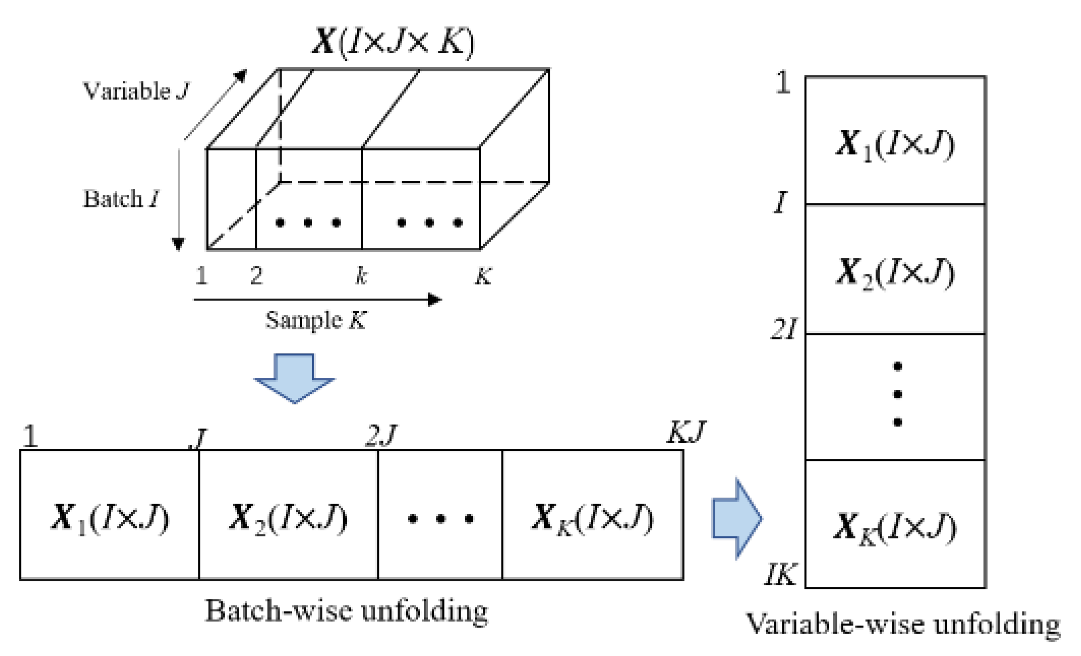
Batch processes produce the same products by the batch-by-batch mode. As one batch operation brings a two-dimensional matrix involving the variable and sample dimension, the training data from multiple batches constitute a three-dimensional matrix $\mathit{X}(I\times J\times K)$, where $I,J,K$ represent the number of batches, variables and samples. This kind of multiway dataset is not directly analyzed because most of the present statistical modeling methods can only deal with a two-dimensional data matrix. Therefore, we need to unfold the three-dimensional data into a two-dimensional matrix and perform the corresponding normalization in the preprocessing stage.

The typical preprocessing method is batch-variable unfolding [13]. Its details are demonstrated in Figure 1. Firstly, the original three-dimensional data matrix $\mathit{X}(I\times J\times K)$ is unfolded along the batch direction into $\mathit{X}(I\times KJ)$. After the batch unfolding, the data are scaled to zero-mean and unit-variance in this direction. Secondly, data are rearranged along the variable direction into $\mathit{X}(IK\times J)$ to highlight the variation of the variables. After these two steps, a two-dimensional matrix is available for the following statistical modeling.

2.2. Overview of SVDD Principle

SVDD is a well-known one-class classification algorithm and has been widely applied to different kinds of anomaly detection tasks [7,28]. Its main idea is to find a minimal hypersphere to enclose as many training samples as possible.

Given the training dataset $\{{\mathit{x}}_i,i=1,2,\cdots ,n\}$, the SVDD optimization objective can be described as [28]

$$\underset{R,\mathit{c},{ϵ}_i}{min}{R}^2+\gamma \sum _{i=1}^n{ϵ}_i$$

(1)

$$s.t.\left|\right|{\mathit{x}}_i-\mathit{c}\left|\right|\le R^2+{ϵ}_i,{ϵ}_i>0,i=1,2,\cdots ,n$$

(2)

where $\mathit{c}$ is the center of the hypersphere, R is the radius of the hypersphere, ${ϵ}_i$ is the slack variable, and $\gamma$ is the trade-off parameter.

The above optimization is under the linear assumption. However, the real process data often have nonlinear relationships. Therefore, a nonlinear mapping function $\mathsf{\Phi }(.)$ is introduced to transform the original data space into a high-dimensional feature space, where the data are linearly related. In this case, the SVDD optimization constraint Equation (2) should be rewritten as

$$s.t.\left|\right|\mathsf{\Phi }\left({\mathit{x}}_i\right)-\mathit{c}\left|\right|\le R^2+{ϵ}_i,{ϵ}_i>0,i=1,2,\cdots ,n$$

(3)

By introducing the Lagrange multiplier, the dual optimization problem is given by [28]

$$\underset{{\alpha }_i,{\alpha }_j}{min}\sum _{i=1}^n{\alpha }_i\mathsf{\Phi }{\left({\mathit{x}}_i\right)}^{\mathrm{T}}\mathsf{\Phi }\left({\mathit{x}}_i\right)-\sum _{i=1}^n\sum _{j=1}^n{\alpha }_i{\alpha }_j\mathsf{\Phi }{\left({\mathit{x}}_i\right)}^{\mathrm{T}}\mathsf{\Phi }\left({\mathit{x}}_j\right)$$

(4)

$$s.t.0\le {\alpha }_i\le \gamma ,\sum _{i=1}^n{\alpha }_i=1.$$

(5)

where ${\alpha }_i,{\alpha }_j$ are the Lagrange multipliers. As the real nonlinear mapping is often unknown, the kernel trick is utilized to deal with the inner production of two nonlinear vectors. This means that

$$\mathsf{\Phi }{\left(\mathit{x}\right)}_i^{\mathrm{T}}\mathsf{\Phi }\left({\mathit{x}}_j\right)=K({\mathit{x}}_i,{\mathit{x}}_j)$$

(6)

where $K(.)$ represents the kernel function operation. In this paper, the common Gaussian kernel function is applied.

To solve the quadratic programming problem in Equations (4) and (5), the hypersphere center is

$$\mathit{c}=\sum _{i=1}^n{\alpha }_i\mathsf{\Phi }\left({\mathit{x}}_i\right)$$

(7)

and the hypersphere radius is

$$R=\left|\right|\mathsf{\Phi }\left({\mathit{x}}_i^{*}\right)-\mathit{c}\left|\right|=\left|\right|\mathsf{\Phi }\left({\mathit{x}}_i^{*}\right)-\sum _{i=1}^n{\alpha }_i\mathsf{\Phi }\left({\mathit{x}}_i\right)\left|\right|$$

(8)

where ${\mathit{x}}_i^{*}$ is any sample corresponding to the $0<{\alpha }_i<C$, which is the so-called support vector.

Given the new testing vector ${\mathit{x}}_t$, its squared distance to the hyphersphere center is used to construct the monitoring index D as [21]

$$D=\left|\right|\mathsf{\Phi }\left({\mathit{x}}_t\right)-\mathit{c}{\left|\right|}^2=K({\mathit{x}}_t,{\mathit{x}}_t)-2\sum _{i=1}^n{\alpha }_{i}K({\mathit{x}}_t,{\mathit{x}}_i)+\sum _{i=1}^n\sum _{j=1}^n{\alpha }_i{\alpha }_{j}K({\mathit{x}}_i,{\mathit{x}}_j)$$

(9)

In the anomaly detection scenario, the monitoring index of normal samples should be smaller than $R^2$. The samples with $D>R^2$ are usually thought to be anomaly points. However, the hypersphere radius R lacks clear statistical significance. By referring to the common practice in data-driven fault diagnosis fields, this paper applies the kernel density estimation technique to determine the 99% confidence limit as the detection threshold $D_{lim}$ [21]. This means that the normal samples have the $D<D_{lim}$ with a 99% confidence level.

2.3. PCA-SVDD Method

Considering that the original process data are correlated and the intrinsic fault features may be covered by noise, PCA is often used to capture the uncorrelated data features [7]. Given the training data matrix $\mathit{X}={[{\mathit{x}}_1{\mathit{x}}_2\cdots {\mathit{x}}_n]}^{\mathrm{T}}\in {\mathcal{R}}^{n\times m}$, it can be decomposed into two parts, namely the principal component matrix $\mathit{T}$ and the residual matrix $\mathit{E}$. The PCA decomposition procedure is formulated as

$$\mathit{X}=\mathit{T}{\mathit{P}}^{\mathrm{T}}+\mathit{E}$$

(10)

where $\mathit{P}\in {\mathcal{R}}^{m\times k}$ is the loading matrix, describing the project directions of the first k principal components.

PCA is integrated with SVDD for the enhanced SVDD model, called PCA-SVDD. In this model, PCA is firstly used to analyze the original training data and then SVDD modeling is carried out on the matrices $\mathit{T}$ and $\mathit{E}$, respectively. For the testing vector ${\mathit{x}}_t$, its principal component vector and residual vector are denoted by ${\mathit{t}}_t$ and ${\mathit{e}}_t$, respectively, which are computed by

$${\mathit{t}}_t={\mathit{x}}_t\mathit{P}$$

(11)

$${\mathit{e}}_t={\mathit{x}}_t-{\mathit{x}}_t\mathit{P}{\mathit{P}}^{\mathrm{T}}$$

(12)

The corresponding two SVDD monitoring indices $D^{\left(t\right)}$ and $D^{\left(e\right)}$ are built as [22]

$$D^{\left(t\right)}=\left|\right|\mathsf{\Phi }\left({\mathit{t}}_t\right)-{\mathit{c}}^{\left(t\right)}{\left|\right|}^2$$

(13)

$$D^{\left(e\right)}=\left|\right|\mathsf{\Phi }\left({\mathit{e}}_t\right)-{\mathit{c}}^{\left(e\right)}{\left|\right|}^2$$

(14)

Different to the basic SVDD method with only one monitoring index on the original data, PCA-SVDD has two monitoring indices for the principal components and residual components, respectively. Their detection thresholds $D_{lim}^{\left(t\right)}$ and $D_{lim}^{\left(e\right)}$ are determined by the kernel density estimation technique. As two uncorrelated subspaces are monitored, PCA-SVDD can investigate the process changes more elaborately.

3. The Proposed DPSVDD Method

3.1. Method Framework

When the traditional SVDD and PCA-SVDD methods are applied to monitor complicated industrial processes, they often neglect the early detection of incipient faults because these methods are only able to extract the shallow features. In order to deal with this issue, this paper proposes one deep probabilistic SVDD (DPSVDD) method by combining the deep learning technology. On the one hand, a typical deep neural network, the convolutional autoencoder, is introduced to mine the deep data features in order to reflect the incipient faulty information more sensitively. On the other, considering that the incipient faults do not lead to a significant fault amplitude but may lead to local probability changes in the data features, this paper applies the Kullback-Leibler (KL) divergence to transform the deep features into probability-related features.

The improved SVDD method has the following framework, shown in Figure 2. According to this figure, the DPSVDD method involves four steps: data preprocessing, deep features extraction, probability analysis and SVDD modeling. After preprocessing, the batch process training data are input into the convolutional autoencoder for the mining of deep features, including the encoder output and reconstruction error. Then, the Kullback-Leibler divergence is applied to extract probability features. Lastly, the SVDD modeling is performed to build the monitoring index.

3.2. Deep Convolutional Feature Extraction

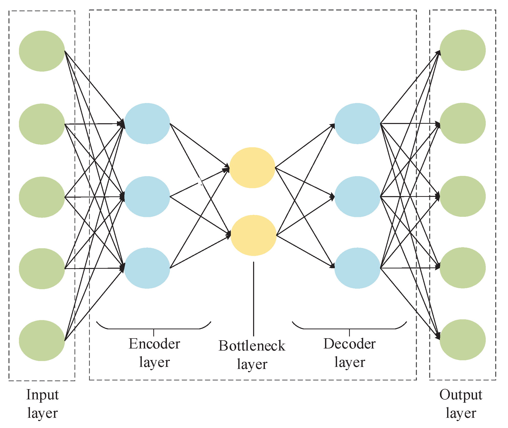
This paper applies the convolutional autoencoder to extract the hidden data representations. The autoencoder is firstly introduced. An autoencoder is a specific unsupervised neural network where the expected outputs are set to be the same as the inputs [29,30]. As shown in Figure 3, usually, one autoencoder network includes five kinds of layers: input layer, encoder layer, bottleneck layer, decoder layer and output layer. The first three parts construct the encoder, which compresses the input data to obtain the main data variations. In some sense, the encoder can be viewed as one nonlinear PCA. The last three parts constitute the decoder, which tries to recover the original input from the extracted features at the bottleneck layer. The optimization objective of the autoencoder is to minimize the reconstruction error between the inputs and the outputs [30]. In the training process, the network parameters are adjusted based on the back propagation of the reconstruction errors.

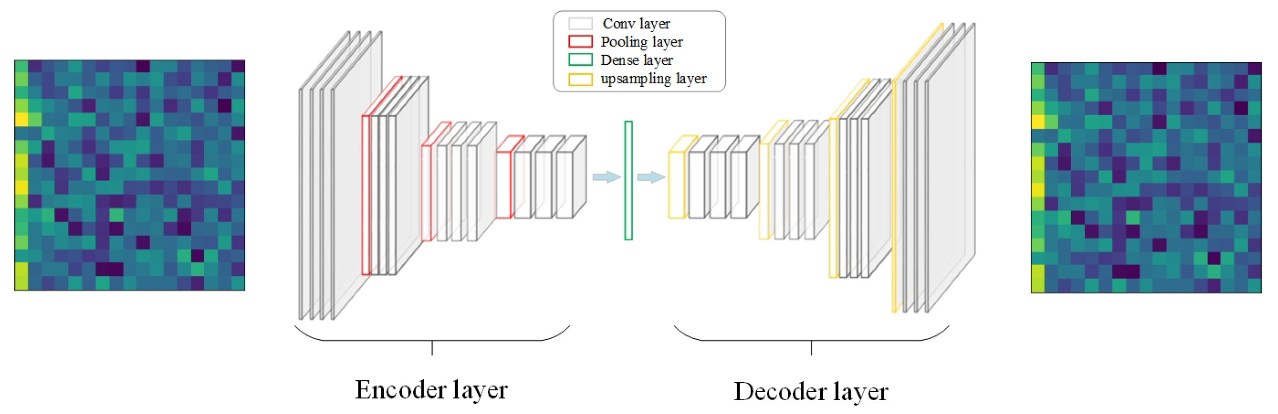
A convolutional autoencoder inherits the feature extraction idea of the basic autoencoder, but it uses the convolutional operation to replace the fully connected operation in the encoder and decoder layers [31]. Due to the use of multiple convolutional layers, the network node number is enlarged. Therefore, the pooling layers are often designed after the convolutional layers. Similarly, the upsampling layers are inserted after the deconvolutional layers. The common convolutional autoencoders include the 1D type and 2D type [31,32]. The 2D convolutional autoencoder preserves the temporal and spatial locality effectively. A typical 2D convolutional autoencoder is shown in Figure 4.

Two main operations in a convolutional autoencoder are convolution and pooling. The convolutional operation applies the convolutional kernel to extract the local features, which can be expressed by

$${\mathit{T}}^{\left(l\right)}=f^{\left(l\right)}(\sum \mathit{X}⨂{\mathit{W}}^{\left(l\right)}+{\mathit{b}}^{\left(l\right)})$$

(15)

where $\mathit{X}$, ${\mathit{T}}^{\left(l\right)}$ stand for the input matrix and the convoluted output matrix, respectively, ⨂ denotes the convolution operation, ${\mathit{W}}^{\left(l\right)}$ stands for the lth convolution kernel, ${\mathit{b}}^{\left(l\right)}$ is the bias corresponding to the ${\mathit{W}}^{\left(l\right)}$. $f^{\left(l\right)}(.)$ is the activation function at the l-th layer. In this paper, the commonly used the Rectified Linear Unit (RELU) function is used.

The pooling operation compresses the data dimension for efficient computation. The pooling layer, also called the subsampling layer, is usually used after the convolutional layer. There are two common types of pooling: max pooling and average pooling. In this paper, average pooling is applied.

Based on a series of convolution and pooling operations, the encoder output, i.e., the bottleneck layer, can be obtained

$$\mathit{T}=encoder(\mathit{X},{\mathit{W}}^{\left(1\right)},\cdots ,{\mathit{W}}^{\left(L_E\right)},{\mathit{b}}^{\left(1\right)},\cdots ,{\mathit{b}}^{\left(L_E\right)})$$

(16)

where $L_E$ is the number of convolutional operations in the encoder.

Similarly, the output of the decoder is obtained based on the deconvolutions and up-samplings by

$$\hat{\mathit{X}}=decoder(\mathit{T},{\tilde{\mathit{W}}}^{\left(1\right)},\cdots ,{\tilde{\mathit{W}}}^{\left(L_D\right)},{\tilde{\mathit{b}}}^{\left(1\right)},\cdots ,{\tilde{\mathit{b}}}^{\left(L_D\right)})$$

(17)

where $\hat{\mathit{X}}$ is the reconstructed input, and $L_D$ is the number of the deconvolutional operations in the decoder.

The mean square error between the original input data and the reconstructed data can be used as the cost function

$$minL=\frac{1}{n}\sum _{k=1}^n\left|\right|\mathit{X}\left(k\right)-\hat{\mathit{X}}\left(k\right){\left|\right|}_F^2$$

(18)

where $\mathit{X}\left(k\right)$, $\hat{\mathit{X}}\left(k\right)$ represent the k-th input image and the corresponding reconstruction image. During the training, the reconstruction error is minimized through optimizing the network weights so that the final weights are optimal as ${\mathit{W}}^{*\left(1\right)},\cdots ,{\mathit{W}}^{*\left(L_E\right)},{\mathit{b}}^{*\left(1\right)},\cdots ,{\mathit{b}}^{*\left(L_E\right)}$, ${\tilde{\mathit{W}}}^{*\left(1\right)},\cdots ,{\tilde{\mathit{W}}}^{*\left(L_D\right)},{\tilde{\mathit{b}}}^{*\left(1\right)},\cdots ,{\tilde{\mathit{b}}}^{*\left(L_D\right)}$.

Based on the CAE, two kinds of features can be obtained for process monitoring. One is the bottleneck layer, also the encoder output, which represents the compressed data variations, while another is the reconstruction error, which represents the remaining residual information.

For the test image data ${\mathit{X}}_t$, the encoder output vector is denoted as ${\mathit{t}}_t$, and the reconstruction error vector is expressed by ${\mathit{e}}_t$. They are expressed by

$${\mathit{t}}_t=encoder({\mathit{X}}_t,{\mathit{W}}^{*\left(1\right)},\cdots ,{\mathit{W}}^{*\left(L_E\right)},{\mathit{b}}^{*\left(1\right)},\cdots ,{\mathit{b}}^{*\left(L_E\right)})$$

(19)

$${\mathit{e}}_t=\frac{1}{d}\sum _{i=1}^d{\mathit{X}}_t(i,:)-{\hat{\mathit{X}}}_t(i,:)$$

(20)

where d is the width size of testing image data, and ${\hat{\mathit{X}}}_t$ is the reconstructed input data as

$${\hat{\mathit{X}}}_t=decoder({\mathit{t}}_t,{\tilde{\mathit{W}}}^{*\left(1\right)},\cdots ,{\tilde{\mathit{W}}}^{*\left(L_D\right)},{\tilde{\mathit{b}}}^{*\left(1\right)},\cdots ,{\tilde{\mathit{b}}}^{*\left(L_D\right)})$$

(21)

By applying SVDD modeling, we can obtain the corresponding CAE-SVDD monitoring indices $D^{\left(t\right)}$ and $D^{\left(e\right)}$. Their detection thresholds are also determined by the kernel density estimation on the training data.

3.3. Probabilistic Monitoring Index Construction

As a deep learning technique, CAE provides more effective features for SVDD modeling. This factually prompts the traditional shallow SVDD model to the deep SVDD model. However, the deep SVDD model based on CAE feature extraction still omits the probability information of the monitored features, which may be helpful in the incipient fault detection. In some incipient fault cases, the probability distribution of features is affected although the amplitude is not significantly changed.

To evaluate the changes in the probability distribution of features, Kullback-Leibler divergence (KLD) is often used. KLD, also called relative entropy, measures the difference in two given probability distributions. For a random variable x, its two continuous probability distribution functions are denoted as $P\left(x\right)$ and $Q\left(x\right)$. The KLD of $P\left(x\right)$ over $Q\left(x\right)$ is expressed by

$$KLD\left(P\right|\left|Q\right)={\int }_{-\infty }^{\infty }P\left(x\right)ln\frac{P\left(x\right)}{Q\left(x\right)}dx$$

(22)

It should be noted that KLD is not a symmetric metric. In other words, the KLD from $P\left(x\right)$ to $Q\left(x\right)$ is not the same as the KLD from $Q\left(x\right)$ to $P\left(x\right)$. In practice, a modified symmetric KLD version is defined as

$$KLD(P,Q)={\int }_{-\infty }^{\infty }P\left(x\right)ln\frac{P\left(x\right)}{Q\left(x\right)}dx+{\int }_{-\infty }^{\infty }Q\left(x\right)ln\frac{Q\left(x\right)}{P\left(x\right)}dx$$

(23)

Under the assumption of Gaussian distribution, the expressions of $P\left(x\right)$ and $Q\left(x\right)$ can be given as

$$P\left(x\right)=\frac{1}{\sqrt{2\pi }\sigma }exp(-\frac{{(x-\mu )}^2}{2{\sigma }^2})$$

(24)

$$Q\left(x\right)=\frac{1}{\sqrt{2\pi }\tilde{\sigma }}exp(-\frac{{(x-\tilde{\mu })}^2}{2{\tilde{\sigma }}^2})$$

(25)

where ${\mu }_j$, ${\sigma }_j$ are the mean and the standard variance of $P\left(x\right)$, and ${\tilde{\mu }}_j$, ${\tilde{\sigma }}_j$ are the mean and the standard variance of $Q\left(x\right)$.

Furthermore, the KLD can be computed as

$$KLD(P\left(x\right),Q\left(x\right))=\frac{1}{2}\left[\frac{{\sigma }_j}{{\tilde{\sigma }}_j}+\frac{{\tilde{\sigma }}_j}{{\sigma }_j}+{({\mu }_j-{\tilde{\mu }}_j)}^2(\frac{1}{\widetilde{{\sigma }_j}}+\frac{1}{{\sigma }_j})-2\right]$$

(26)

In the fault detection scenario, we can utilize $Q\left(x\right)$ as the reference probability distribution, while applying the $P\left(x\right)$ as the tested probability distribution. If these two probability distributions are the same, i.e., $P\left(x\right)=Q\left(x\right)$, there exists $KLD\left(P\right|\left|Q\right)=0$. Otherwise, $KLD\left(P\right|\left|Q\right)>0$. Therefore, KLD can be used to investigate the deviations of monitored variables. In this paper, we apply the KLD to measure the probability changes of the deep features ${\mathit{t}}_t=[t_{t,1},t_{t,2},\cdots ,]$ and ${\mathit{e}}_t=[e_{t,1},e_{t,2},\cdots ]$, so that the probability-related features are expressed by

$$t_i^{KLD}=KLD(P\left(t_{t,i}\right),Q\left(t_{t,i}\right))$$

(27)

$$e_i^{KLD}=KLD(P\left(e_{t,i}\right),Q\left(e_{t,i}\right))$$

(28)

where $t_i^{KLD}$, $e_i^{KLD}$ are the probability-related features corresponding to the encoder output $t_i$ and the reconstruction error $e_i$. Further, building the SVDD models based on these probability-related features will yield deep probabilistic SVDD models.

4. Batch Process Monitoring Procedure

The monitoring procedure based on DPSVDD includes two phases: offline modeling and online monitoring. In the first phase, process training data of multiple batches are collected to build the DPSVDD model, while the online new data are projected onto the developed model in the second phase. The monitoring indices are compared with their threshold to indicate whether a fault occurs. The whole procedure is detailed below.

Offline modeling phase:

• Collect the offline training data from the batch process and perform the preprocessing using the batch-variable mode.
• Apply the deep convolutional autoecoder to extract the encoder output and the reconstruction errors as the process deep features.
• Compute the probability-related features by the KL divergence corresponding to the training data.
• Build SVDD models based on the probability-related features of training data.
• Compute the detection threshold of monitoring indices.

Online detection phase:

• Collect the online new data vector and preprocess it based on the training data.
• Project the preprocessed data onto CAE and obtain the corresponding features.
• Compute the probability-related features by the KL divergence for the new data.
• Calculate the monitoring indices of the new data vector.
• Compare the monitoring indices with the corresponding detection threshold and judge the process status.

It should be noted that the above procedure does not consider the model updating. In real applications, when the engineers judge that the current model cannot reflect the normal operations, so that high rates of missing detection or false alarms occur, the monitoring model should be updated.

5. Case Study

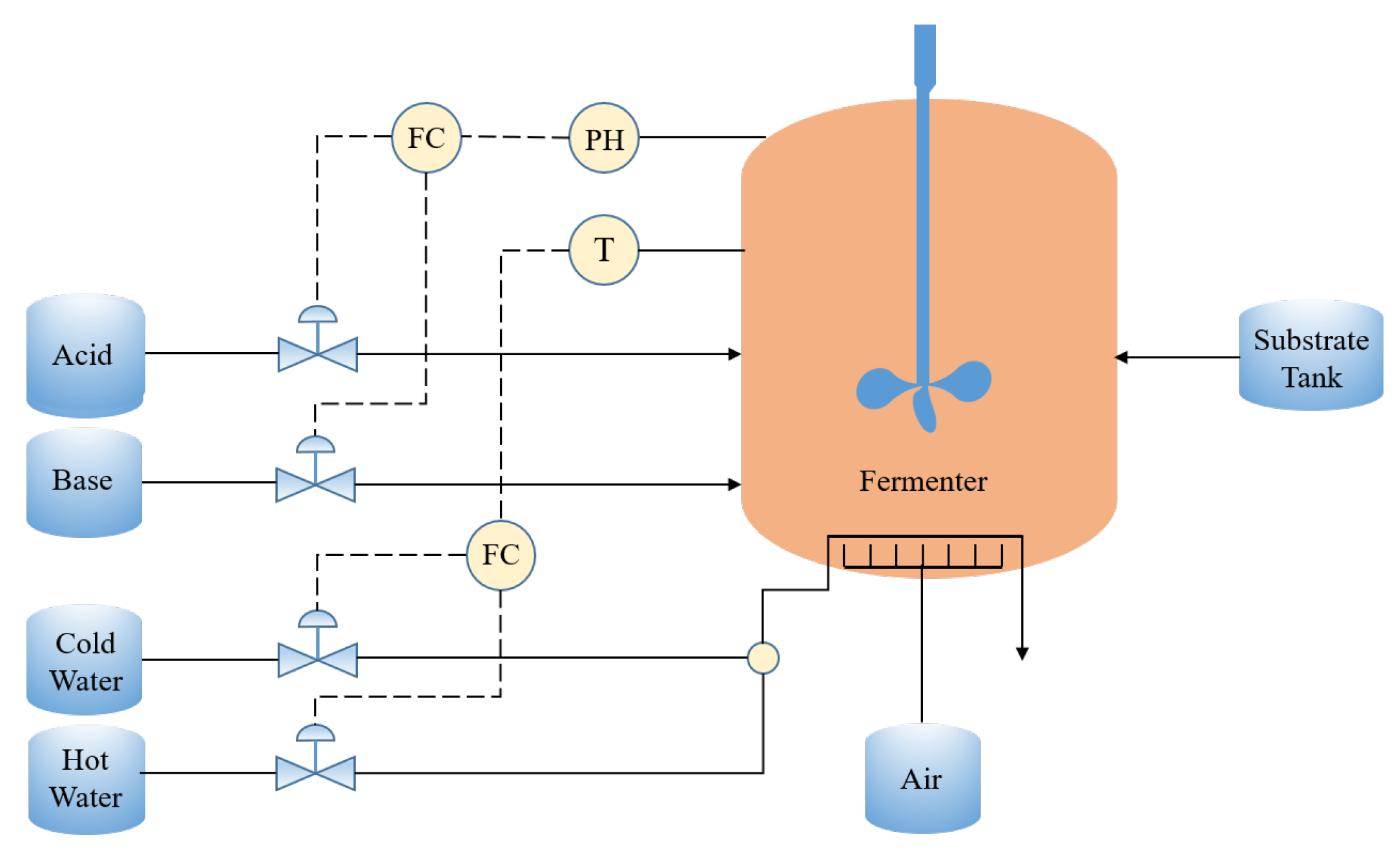
A case study on the penicillin fermentation process is given in this section. The penicillin fermentation process is a complex biochemical reaction system with batch operations and has been widely used as the benchmark objective for testing different batch process monitoring methods [11,33,34]. A diagram of a penicillin fermentation reactor is shown in Figure 5. This process consists of two main operating stages: the pre-culture stage and batch feeding stage. During the initial pre-culture phase, a large number of the nutrients necessary for cells are produced and penicillin cells appear during the period of exponential growth. In order to maintain a high yield of penicillin in the batch feeding stage, a continuous supply of glucose to the fermentation process is needed to keep the biomass growth rate constant. In order to provide the best conditions for the production of penicillin, the temperature and pH of the fermenter are controlled in two closed control loops.

The process simulation is performed based on the software Pensim V2.0 [35]. In the simulation procedure, we collect 17 measurements as monitoring variables. Gaussian noises are added in the variable collection procedure. Thirty batches of normal operation data are collected to form the modeling data set, where each batch consists of 400 h with a sampling time of 0.5 h. This means that each dataset has 800 samples. In this paper, the simulated normal operation data belong to the same operation mode. It is assumed that all the used 30 batches are enough to describe the normal data changes sufficiently. Besides the normal operation case, we also simulate six batches of faulty operations. The detailed fault cases are listed in

Table 1. Six fault patterns in the penicillin fermentation process.

No.	Fault Variable	Fault Type	Fault Amplitude	Lasting Time (h)
F1	Aeration rate	Step	5%	101–400
F2	Aeration rate	Ramp	0.5	101–400
F3	Agitator rate	Step	1%	101–400
F4	Agitator rate	Ramp	0.45	101–400
F5	Substrate feed rate	Step	6%	101–400
F6	Substrate feed rate	Ramp	0.003	101–400

, which includes the step change and slope change in the aeration rate, agitator power and substrate feeding rate.

The proposed method is compared with the other four methods: SVDD, PCA-SVDD, AE-SVDD, CAE-SVDD. Among these methods, SVDD is the basic method. In the other methods of PCA-SVDD, AE-SVDD, CAE-SVDD, different feature extraction layers are designed. The proposed method not only considers the deep feature extraction, but also utilizes the probability information to enhance the incipient fault detection. For the SVDD method, the Gaussian kernel width is used and the trade-off parameter $\gamma$ is set to 0.05. When PCA is applied, the retained principal component number is determined by the rule of 85% cumulative percentage of variance. In the AE-SVDD, the node number of the bottleneck layer is set to 5. The CAE-SVDD is slightly complicated. As 2D-CAE is used, the moving window $17\times 17$ is used to construct the 2D data image. The detailed CAE network structure parameters are listed in

Table 2. Network structure parameters in CAE-SVDD.

No.	Parameters	Value
1	input patch size	17×17
2	filter number and size in 1st convolution Layer	8, $3\times 1$
3	size in 1st average pooling layer	$2\times 1$
4	filter number and size in 2nd convolution Layer	4, $3\times 1$
5	size in 2nd average pooling layer	$2\times 1$
6	filter number and size in 3rd convolution Layer	1, $1\times 3$
7	size in 3rd average pooling layer	$1\times 2$
8	filter number and size in 1st deconvolution Layer	4, $1\times 3$
9	size in 1st upsampling layer	$1\times 2$
10	filter number and size in 2nd deconvolution Layer	2, $1\times 3$
11	size in 2nd upsampling layer	$2\times 1$
12	filter number and size in 3rd deconvolution Layer	8, $1\times 3$
13	size in 3rd upsampling layer	$2\times 1$
14	filter number and size in 4th deconvolution Layer	16, $3\times 1$
15	filter number and size in 5th deconvolution Layer	1, $2\times 2$

.

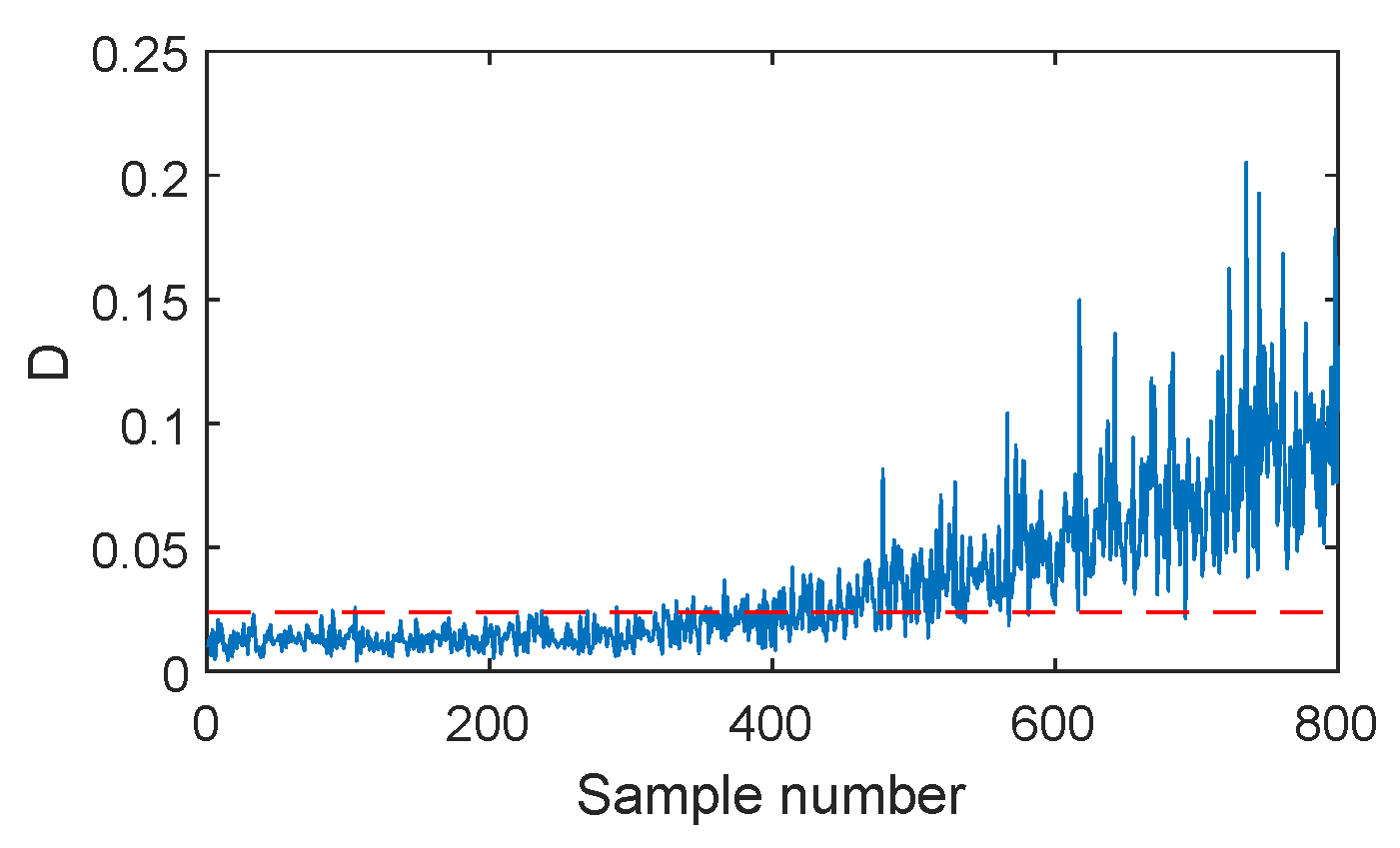
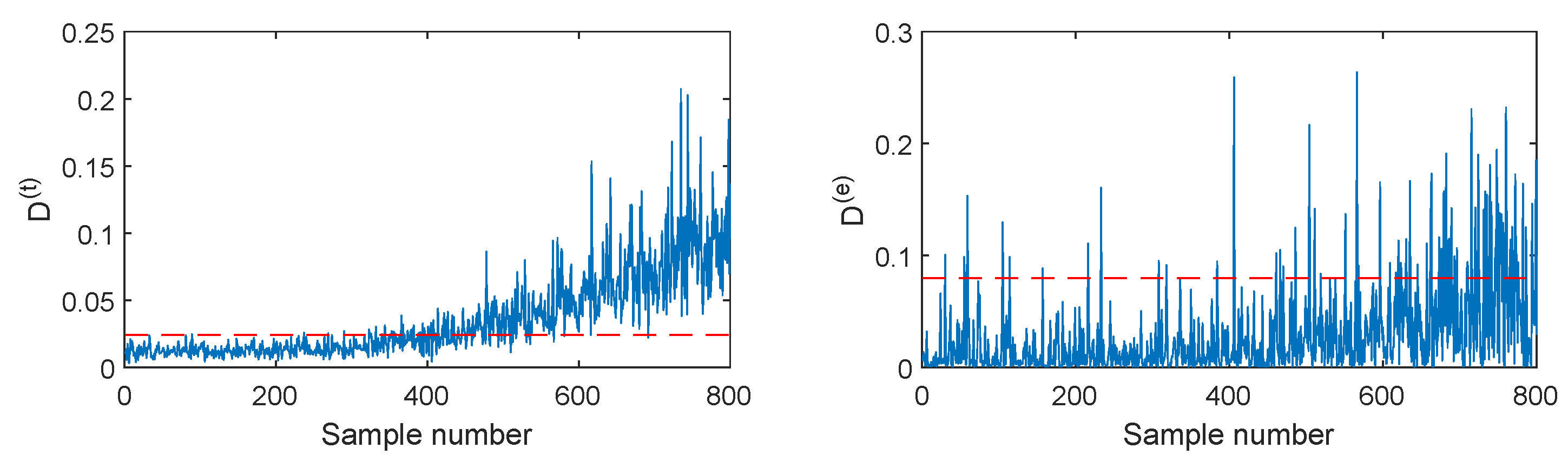
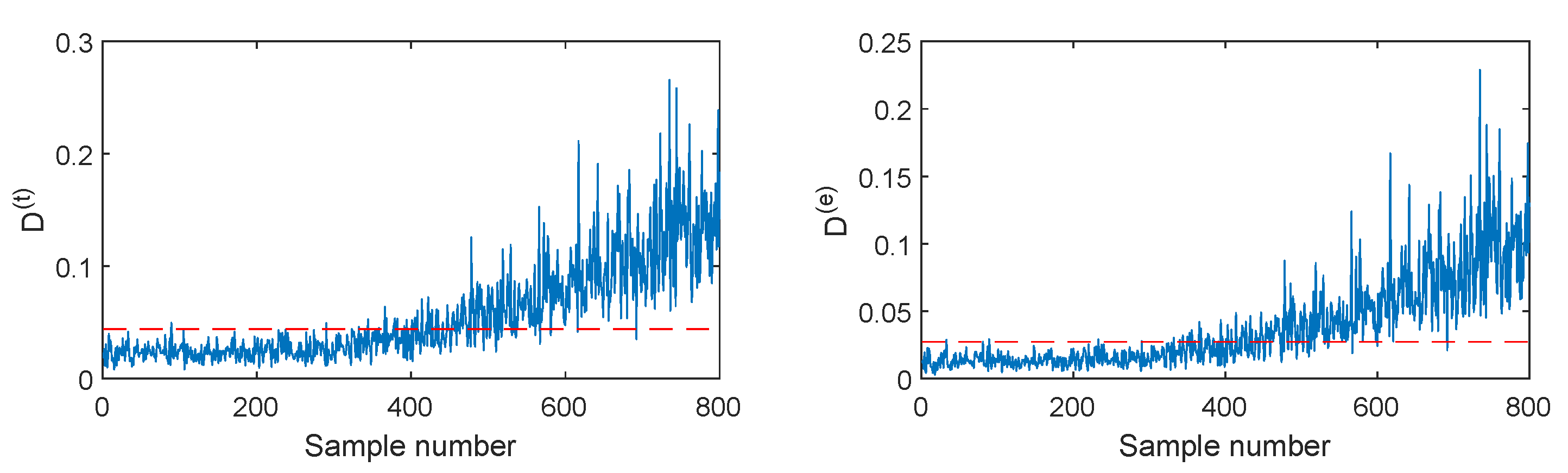
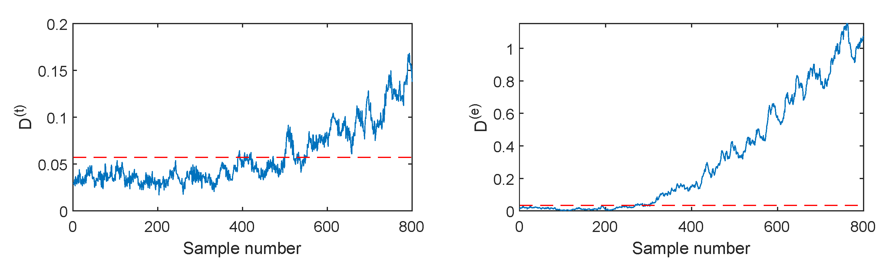
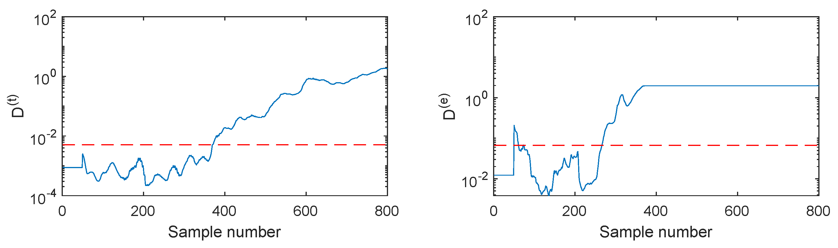
The fault F2 is firstly illustrated, which is the ramp change in the aeration rate with the slope of +(0.5 L/h)/100 h. The monitoring results of different methods are listed in Figure 6, Figure 7, Figure 8, Figure 9 and Figure 10. When SVDD is applied to monitor this fault, its monitoring chart is shown in Figure 6, where the monitoring index D alarms until the 400-th sample with the fault detection rate of 61%. Due to the strong noise and the slow speed of the incipient fault, SVDD cannot detect this fault sensitively. By applying PCA for feature extraction, the PCA-SVDD monitoring chart in Figure 7 gives a fault detection rate of 62% and 12% for the monitoring indices $D^{\left(t\right)}$ and $D^{\left(e\right)}$, respectively. This result is slightly superior to the SVDD’s. Further, using the autoencoder for nonlinear principal component extraction, AE-SVDD achieves fault detection rates of 58.5% and 61.67% for the two monitoring indices, respectively. Compared to PCA-SVDD, AE-SVDD improves the monitoring results of $D^{\left(e\right)}$ significantly. Although these three methods have a slight performance difference, none of them can detect this fault effectively. With the strong aid of the convolutional autoencoder in mining deep features, CAE shows a clear improvement, as shown in Figure 9. In particular, the index $D^{\left(e\right)}$ of CAE-SVDD detects the fault at the 270-th sample. Its fault detection rate reaches 87.17%. However, its $D^{\left(t\right)}$ index gives a poor fault detection rate of 48.5%, which is even lower than the basic SVDD’s. By further considering the probability information of deep features, as shown in Figure 10, the $D^{\left(t\right)}$ index of DPSVDD enhances the detection performance to 71.83%, while the $D^{\left(e\right)}$ retains a high fault detection rate of 89.17%. The testing results on the fault F2 demonstrate that the CAE-SVDD can improve the monitoring performance of incipient faults effectively, and the proposed DPSVDD can lead to a further enhancement.

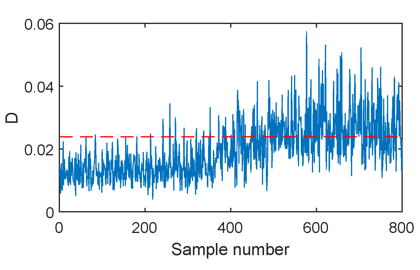
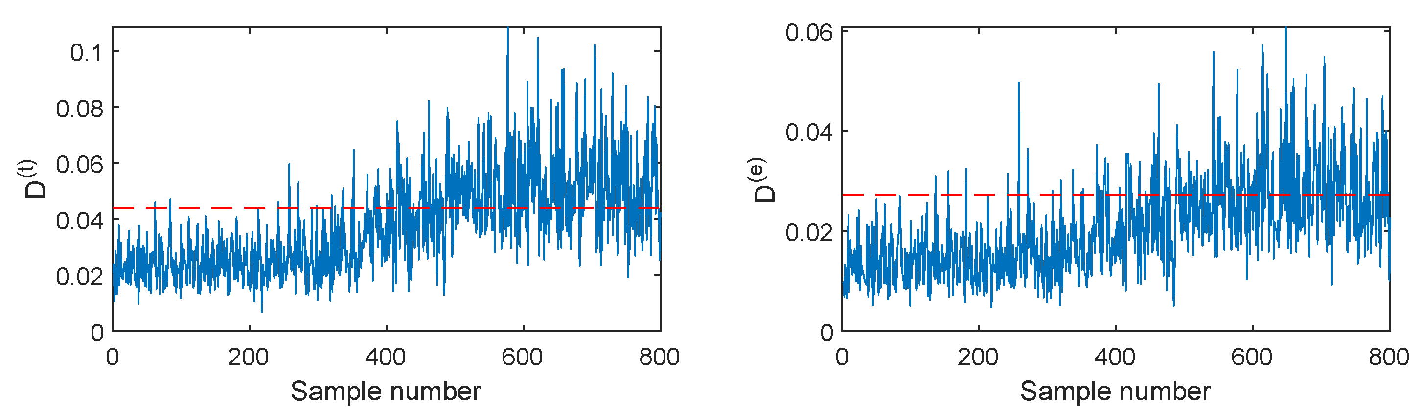
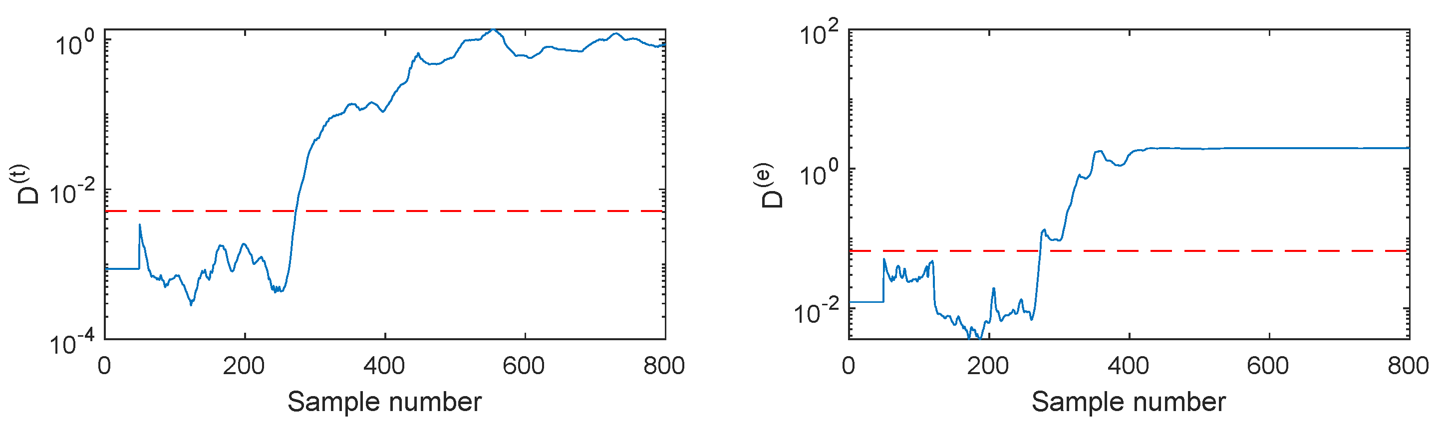
Another illustrated case is fault F5, which involves a 6% step change in the substrate feed rate. When this fault occurs, the SVDD D index in Figure 11 fluctuates around the detection threshold and cannot indicate the fault clearly. Its fault detection rate is only 37.5%. When using PCA-SVDD in Figure 12, the detection results are still unsatisfactory because its fault detection rates are 37% and 3.67%, respectively. Therefore, the linear features cannot reflect this incipient fault effectively. By utilizing the autoencoder for the capture of nonlinear features, the AE-SVDD monitoring charts in Figure 13 obtain a slight performance improvement, with fault detection rates of 40.5% and 28.33% for $D^{\left(t\right)}$ and $D^{\left(e\right)}$, respectively. With further mining of the deep convolutional features, CAE-SVDD can detect this fault clearly, as shown in Figure 14, where the $D^{\left(t\right)}$’s detection rate is 79.5%, while the $D^{\left(e\right)}$’s detection rate is 88.5%. The CAE-SVDD gives around a 40% and 60% increment in terms of the fault detection rate, which shows the advantage of convolutional features. When DPSVDD is applied in Figure 15, its $D^{\left(e\right)}$ index displays a similar performance to that of CAE-SVDD. However, the $D^{\left(t\right)}$ index of DPSVDD achieves an 88% detection rate, which is 8.5% higher than the CAE-SVDD $D^{\left(t\right)}$’s. In general, the proposed DPSVDD method has the best monitoring performance in terms of the monitoring of fault F5.

All the fault monitoring results on the six faults are summarized in

Table 3. Fault detection rates (FDRs)(%) of the six tested faults by the five compared methods.

Method	SVDD	PCA-SVDD		AE-SVDD		CAE-SVDD		DPSVDD
Index	$\mathit{D}$	${\mathit{D}}^{\left(\mathit{t}\right)}$	${\mathit{D}}^{\left(\mathit{e}\right)}$	${\mathit{D}}^{\left(\mathit{t}\right)}$	${\mathit{D}}^{\left(\mathit{e}\right)}$	${\mathit{D}}^{\left(\mathit{t}\right)}$	${\mathit{D}}^{\left(\mathit{e}\right)}$	${\mathit{D}}^{\left(\mathit{t}\right)}$	${\mathit{D}}^{\left(\mathit{e}\right)}$
F1	27.50	30.33	3.50	22.33	26.50	17.17	98.83	91.33	96.83
F2	61.00	62.00	12.00	58.50	61.67	48.50	87.17	71.83	89.17
F3	8.83	8.17	4.17	8.00	7.83	85.17	92.83	96.17	93.50
F4	57.17	55.17	24.50	56.17	55.33	81.83	82.83	89.50	82.67
F5	37.50	37.00	3.67	40.50	28.33	79.50	88.50	88.00	87.83
F6	53.50	54.17	7.33	55.50	50.00	66.83	72.33	76.67	72.33
Mean	40.92	41.14	9.19	40.17	38.28	63.17	87.08	85.58	87.06

and

Table 4. False alarm rates (FARs)(%) of the six tested faults by the five compared methods.

Method	SVDD	PCA-SVDD		AE-SVDD		CAE-SVDD		DPSVDD
Index	$\mathit{D}$	${\mathit{D}}^{\left(\mathit{t}\right)}$	${\mathit{D}}^{\left(\mathit{e}\right)}$	${\mathit{D}}^{\left(\mathit{t}\right)}$	${\mathit{D}}^{\left(\mathit{e}\right)}$	${\mathit{D}}^{\left(\mathit{t}\right)}$	${\mathit{D}}^{\left(\mathit{e}\right)}$	${\mathit{D}}^{\left(\mathit{t}\right)}$	${\mathit{D}}^{\left(\mathit{e}\right)}$
FAR	1.25	1.17	1.08	1.25	1.00	1.33	0.42	0.92	3.0

. In Table 3, it can be observed that the mean fault detection rates of SVDD D and PCA-SVDD $D^{\left(t\right)}$ are both around 40%. However, the PCA-SVDD $D^{\left(e\right)}$ index can provide a good supplement for incipient monitoring, although its monitoring performance is not satisfactory, with a low mean fault detection rate of 9.19%. As AE-SVDD is used, the $D^{\left(e\right)}$ index is strengthened so that the mean fault detection rate reaches 38.28%. For CAE-SVDD, its mean fault detection rates of the two monitoring indices are 63.17% and 87.08%, respectively, which are obviously higher than those of other methods. With the consideration of probability information, the DPSVDD further improves the mean detection rate of $D^{\left(t\right)}$ so that both indices provide higher mean fault detection rates of over than 80%. As for each testing dataset, the first 200 samples represent the normal operation status. In the ideal case, there should be no alarms when monitoring the normal samples. To evaluate the false alarm rates of the different methods, the results are listed in Table 4. From this table, we can see that all the FARs are around 1%. This is consistent with the use of the 99% confidence limit. However, it should be noted that the false alarm rate of DPSVDD $D^{\left(e\right)}$ is slightly higher than the other methods. Further, considering that no significant improvement can be found in terms of the fault detection rate, in practice, we can only perform the probability analysis on the $D^{\left(t\right)}$ index.

In the above discussion, the proposed method is only applied to detect whether a fault occurs. However, it cannot identify the type of fault that occurs. In fact, a complete fault diagnosis system contains two features, namely fault detection and fault pattern recognition. This paper only focuses on the former. The latter is also a valuable task that deserves future study because it is important in carrying out fault recovery actions.

6. Conclusions

Timely fault detection is important to the safe running of batch processes. In order to detect incipient faults sensitively, this paper developed an improved SVDD monitoring method by integrating deep convolutional feature extraction and probability analysis. The contributions include two aspects. On the one hand, a deep SVDD model is built based on the convolutional autoencoder for mining the temporal-spatial data features sufficiently. On the other hand, based on the extracted deep features, probability distribution differences between the real-time data and the modeling data are measured by KL divergence so that the probability-related deep features are obtained for the following SVDD monitoring indices’ construction. The validation on the penicillin fermentation process shows that the proposed method can provide more sensitive detection of incipient faults.

Although a significant performance improvement is achieved by the proposed method, it still encounters some challenges. The first is the issue of how to deal with the multimode and multistage properties of batch processes. In this paper, a single global SVDD model is built, which may be not sufficient for some complicated batch processes. In the future, it is necessary to study the sub-model techniques for effectively handling the mutlimode and multistage characteristics. Another problem is the deep network parameter optimization. In this paper, the deep network structure and parameters are determined by user experience. The question of how to optimize them is deserving of further discussion.

References

- Yu, W.; Zhao, C.; Huang, B. Stationary subspace analysis-based hierarchical model for batch processes monitoring. IEEE Trans. Control Syst. Technol. 2021, 29, 444–453. [Google Scholar] [CrossRef]
- Zhang, H.; Deng, X.; Zhang, Y.; Hou, C.; Li, C. Dynamic nonlinear batch process fault detection and identification based on two-directional dynamic kernel slow feature analysis. Can. J. Chem. Eng. 2021, 99, 306–333. [Google Scholar] [CrossRef]
- Rendall, R.; Chiang, L.H.; Reis, M.S. Data-driven methods for batch data analysis–A critical overview and mapping on the complexity scale. Comput. Chem. Eng. 2019, 124, 1–13. [Google Scholar] [CrossRef]
- Jiang, Q.; Yan, S.; Yan, X.; Yi, H.; Gao, F. Data-driven two-dimensional deep correlated representation learning for nonlinear batch process monitoring. IEEE Trans. Ind. Inform. 2020, 16, 2839–2848. [Google Scholar] [CrossRef]
- Taqvi, S.A.A.; Zabiri, H.; Tufa, L.D.; Uddin, F.; Fatima, S.A.; Maulud, A.S. A review on data-driven learning approaches for fault detection and diagnosis in chemical processes. ChemBioEng Rev. 2021. [Google Scholar] [CrossRef]
- Zhang, Z.; Deng, X. Anomaly detection using improved deep SVDD model with data structure preservation. Pattern Recognit. Lett. 2021, 148, 1–6. [Google Scholar] [CrossRef]
- Deng, X.; Zhang, Z. Nonlinear chemical process fault diagnosis using ensemble deep support vector data description. Sensors 2020, 20, 4599. [Google Scholar] [CrossRef] [PubMed]
- Ge, Z.; Song, Z. Semiconductor manufacturing process monitoring based on adaptive substatistical pca. IEEE Trans. Semicond. Manuf. 2010, 23, 99–108. [Google Scholar]
- Pimentel, P.; Fern, A.; Peres, T.N.; Anzanello, M.J. Fault detection in batch processes through variable selection integrated to multiway principal component analysis. J. Process Control 2019, 80, 223–234. [Google Scholar]
- Yao, M.; Wang, H. On-line monitoring of batch processes using generalized additive kernel principal component analysis. J. Process Control 2015, 28, 56–72. [Google Scholar] [CrossRef]
- Gao, X.; Xu, Z.; Li, Z.; Wang, P. Batch process monitoring using multiway Laplacian autoencoders. Can. J. Chem. Eng. 2020, 98, 1269–1279. [Google Scholar] [CrossRef]
- Zhang, S.; Zhao, C. Slow-feature-analysis-based batch process monitoring with comprehensive interpretation of operation condition deviation and dynamic anomaly. IEEE Trans. Ind. Electron. 2019, 66, 3773–3783. [Google Scholar] [CrossRef]
- Zhang, H.; Tian, X.; Deng, X.; Cao, Y. Batch process fault detection and identification based on discriminant global preserving kernel slow feature analysis. ISA Trans. 2018, 79, 108–126. [Google Scholar] [CrossRef]
- Cao, Y.; Hu, Y.; Deng, X.; Tian, X. Quality-relevant batch process fault detection using a multiway multi-subspace cva method. IEEE Access 2017, 5, 23256–23265. [Google Scholar] [CrossRef]
- Ge, Z.; Gao, F.; Song, Z. Batch process monitoring based on support vector data description method. J. Process Control 2011, 21, 949–959. [Google Scholar] [CrossRef]
- Yao, M.; Wang, H.; Xu, W. Batch process monitoring based on functional data analysis and support vector data description. J. Process Control 2014, 24, 1085–1097. [Google Scholar] [CrossRef]
- Lv, Z.; Yan, X. Hierarchical support vector data description for batch process monitoring. Ind. Eng. Chem. Res. 2016, 55, 9205–9214. [Google Scholar] [CrossRef]
- Wang, J.; Qiu, K.; Liu, W.; Yu, T.; Zhao, L. Unsupervised-multiscale-sequential-partitioning and multiple-svdd-model-based process-monitoring method for multiphase batch processes. Ind. Eng. Chem. Res. 2018, 57, 17437–17451. [Google Scholar] [CrossRef]
- Lv, Z.; Yan, X.; Jiang, Q.; Li, N. Just-in-time learning-multiple subspace support vector data description used for non-Gaussian dynamic batch process monitoring. J. Chemom. 2019, 33, e3134. [Google Scholar] [CrossRef]
- Zhang, M.; Yi, Y.; Chen, W. Multistage condition monitoring of batch process based on multi-boundary hypersphere svdd with modifed bat algorithm. Arab. J. Sci. Eng. 2021, 46, 1647–1661. [Google Scholar] [CrossRef]
- Wang, X.; Wang, Y.; Deng, X.; Cao, Y. A batch process monitoring method using two-dimensional localized dynamic support vector data description. IEEE Access 2020, 8, 181192–181204. [Google Scholar] [CrossRef]
- Li, G.; Hu, Y.; Chen, H.; Shen, L.; Li, H.; Hu, M.; Liu, J.; Sun, K. An improved fault detection method for incipient centrifugal chiller faults using the PCA-R-SVDD algorithm. Energy Build. 2016, 116, 104–113. [Google Scholar] [CrossRef]
- Zhang, Y.; Li, X. Two-step support vector data description for dynamic, non-linear, and non-Gaussian processes monitoring. Can. J. Chem. Eng. 2020, 98, 2109–2124. [Google Scholar] [CrossRef]
- Wang, Z.; Li, S.; Song, H.; Zhou, X. Monitoring based on MIC-PCA and SVDD for industrial process. In Proceedings of the 2017 IEEE 2nd Advanced Information Technology, Electronic and Automation Control Conference, Chongqing, China, 25–26 March 2017; pp. 1210–1214. [Google Scholar]
- Wang, H.; Liu, C.; Jiang, D.; Jiang, Z. Collaborative deep learning framework for fault diagnosis in distributed complex systems. Mech. Syst. Signal Process. 2021, 156, 107650. [Google Scholar] [CrossRef]
- Otter, D.W.; Medina, J.R.; Kalita, J.K. A survey of the usages of deep learning for natural language processing. IEEE Trans. Neural Netw. Learn. Syst. 2021, 32, 604–624. [Google Scholar] [CrossRef] [Green Version]
- Sengupta, S.; Basak, S.; Saikia, P.; Paul, S.; Tsalavoutis, V.; Atiah, F.; Ravi, V.; Peters, A. A review of deep learning with special emphasis on architectures, applications and recent trends. Knowl. Based Syst. 2020, 194, 105596. [Google Scholar] [CrossRef] [Green Version]
- Tax, D.M.J.; Duin, R.P.W. Support vector data description. Mach. Learn. 2004, 54, 45–66. [Google Scholar] [CrossRef] [Green Version]
- Majumdar, A. Kernelized linear autoencoder. Neural Process. Lett. 2021, 53, 1597–1614. [Google Scholar] [CrossRef]
- Lin, G.; Fan, C.; Chen, W.; Chen, Y.; Zhao, F. Class label autoenocoder with structure refinement for zero-shot learning. Neurocomputing 2021, 428, 54–64. [Google Scholar] [CrossRef]
- Palsson, B.; Ulfarsson, M.O.; Sveinsson, J.R. Convolutional autoencoder for spectral spatial hyperspectral unmixing. IEEE Trans. Geosci. Remote Sens. 2021, 59, 535–549. [Google Scholar] [CrossRef]
- Yu, J.; Zhou, X. One-dimensional residual convolutional autoencoder based feature learning for gearbox fault diagnosis. IEEE Trans. Ind. Inform. 2020, 16, 6347–6358. [Google Scholar] [CrossRef]
- Zhou, Y.; Xu, K.; He, F.; He, D. Nonlinear fault detection for batch process via improved chordal kernel tensor locality preserving projections. Control Eng. Pract. 2020, 101, 104514. [Google Scholar] [CrossRef]
- Chang, P.; Ding, C.; Zhao, Q. Fault diagnosis of microbial pharmaceutical fermentation process with non-Gaussian and nonlinear coexistence. Chemom. Intell. Lab. Syst. 2020, 199, 103931. [Google Scholar]
- Birol, G.; Undey, C.; Cinar, A. A modular simulation package for fed-batch fermentation: Penicillin production. Comput. Chem. Eng. 2002, 26, 1553–1565. [Google Scholar] [CrossRef]
Figure 1.
Batch-variable unfolding procedure.
Figure 2.
The proposed method framework.
Figure 3.
The autoencoder structure.
Figure 4.
The convolutional autoencoder structure.
Figure 5.
The penicillin fermentation reactor diagram.
Figure 6.
SVDD monitoring charts for fault F2.
Figure 7.
PCA-SVDD monitoring charts for fault F2.
Figure 8.
AE-SVDD monitoring charts for fault F2.
Figure 9.
CAE-SVDD monitoring charts for fault F2.
Figure 10.
DPSVDD monitoring charts for fault F2.
Figure 11.
SVDD monitoring charts for fault F5.
Figure 12.
PCA-SVDD monitoring charts for fault F5.
Figure 13.
AE-SVDD monitoring charts for fault F5.
Figure 14.
CAE-SVDD monitoring charts for fault F5.
Figure 15.
DPSVDD monitoring charts for fault F5.