A Sequential Optimization-Simulation Approach for Planning the Transition to the Low Carbon Freight System with Case Study in the North Island of New Zealand

Abstract

Freight movement has always been, and always will be an essential activity. Freight transport is one of the most challenging sectors to transition to net-zero carbon. Traffic assignment, mode allocation, network planning, hub location, train scheduling and terminal design problem-solving have previously been used to address cost and operation efficiencies. In this study, the interdisciplinary transition innovation, management and engineering (InTIME) methodology was used for the conceptualization, redesign and redevelopment of the existing freight systems to achieve a downshift in fossil energy consumption. The fourth step of the InTIME methodology is the conceptualization of a long-term future intermodal transport system that can serve the current freight task. The novelty of our approach stands in considering the full range of freight supply chain factors as a whole, using an optimization-simulation approach as if we were designing the low-carbon system of 2121. For the optimization, ArcGIS software was used to set up a multimodal network model. Route and mode selection were delivered through the optimization of energy use within the network. Complementarily, Anylogic software was used to build a GIS-based discrete event simulation model and set up different experiments to enhance the solution offered by the network analysis. The results outline the resources needed (i.e., number of railway tracks, train speed, size of railyards, number of cranes and forklifts at terminals) to serve the freight task. The results can be backcast to reveal the most efficient investments in the near term. In the case of New Zealand’s North Island, the implementation of strategic terminals, with corresponding handling resources and railyards, could deliver 47% emissions reduction from the sector by 2030, ahead of longer lead-time upgrades like electrification of the railway infrastructure.

1. Introduction

In 2017, world primary energy consumption reached 9718 Mtoe (million tons of oil equivalent) and the transportation sector was responsible for 27.9% of the total energy demand [1]. Greenhouse gas (GHG) emissions from the transport sector have been increasing at a faster pace than in any other sector, and if current trends are maintained, it is expected that emissions will be double the current levels (7 Gt CO₂eq in 2010) by 2050 [2].

The energy transition of the transport sector is critical since almost all means of transport are heavily dependent on fossil fuels. The strong reliance that the transport sector has on the oil market poses a threat to the future accessibility of essential activities and commodities, due to the finite nature of this resource, its environmental implications and high price volatility [3]. Transitioning the freight transport system is likely to involve a reconfiguration of the broader supply chain. The elaboration of the whole system reconfiguration would require a conceptualization phase that encompasses multiple change mechanisms rather than isolated disruptive niche innovations [4]. Whole-system analysis of freight transportation includes multiple transport regimes (modal shift to greener modes) as well as niche innovations (vehicle technologies, substitution of energy carriers, relaxation of just-in-time deliveries and localized sourcing) [4,5].

Current freight intermodal systems have developed organically without a high-level master plan for low carbon. GHG emissions are to a large extent dependent on the choice and design of infrastructure [6], yet policy actions on freight infrastructure investment still prioritize travel time and reliability attributes [7], advantaging truck transportation over alternative modes. Road freight is very difficult to decarbonize without a complete redevelopment of the vehicles, infrastructure, and energy supply [6]. A dramatic reduction of carbon emissions as part of affordable long-term national supply chains will require near-term investments and interventions by the government and firms. The methods for identifying these investments and delivering freight transport policies are mainly based on perspectives from economic geography, transport engineering and operations research disciplines. Linkages amongst these disciplines are developing, yet there is not a widely accepted unifying theoretical framework [8]. Recent freight modeling approaches have complemented the conventional 4-step model [9] with logistic decision-making aspects [10,11]. Decision-making involves logistic models [12] that are often calibrated through transport surveys reflecting the status quo, which prioritize cost and transit time over environmental considerations. Conventional energy planning is informed by scenario-based approaches that consider a portfolio of interventions against business-as-usual trajectories [13]. Investment risk is associated with high capital expenditure requirements. Furthermore, decisions are challenged by the uncertainty of future environmental, technological, socio-economic, and political conditions. Urgent infrastructure investments are needed to decarbonize freight transport [6]. Planners and investors need new decision support tools that deliver freight efficiency and low GHG emissions through infrastructure development. Our work aims to fill the gap in long-term decision support through transition engineering.

Transition engineering is emerging in response to complex global problems like climate change and resource depletion. The approach is similar to the design thinking employed for product innovation but uses a very long-term perspective to trigger insight into projects with the potential to change the business-as-usual trajectory. The seven steps of the interdisciplinary transition innovation, management and engineering (InTIME) methodology [14] are described in Appendix A. The InTIME methodology has previously led to an innovative personal transport audit and survey of adaptive capacity of personal car trips in cities [15]. The focus of the methodology on the disruption of existing travel demand patterns led to insights into risk assessment for essential activities to fuel supply shocks as a function of urban form [16]. Changes in land use, options for infrastructure, property development and technology investment incentives have been shown to have the potential to downshift the oil dependency of a city and build resilience [15,16,17].

The foremost challenge in the InTIME methodology is developing a “path-break concept” of how the zero net carbon freight supply chain system of 2121 will work (Step 4 in Figure A1). The purpose of a path-break concept for freight transport systems is to facilitate engineers to explore the configuration, capacity and resources needed by a system to meet the essential freight duty, while achieving fossil-fuel reduction targets. The path-break concept is not merely a scenario. It is an engineering system design of a specific freight supply chain under the COP21 Paris Agreement conditions, primarily that there be no fossil oil available for trucks on the road. Developing a path-break concept is challenging for several reasons. There is no reliable data about 2021 other than geographical base data, the current freight demand, and the possible longevity of existing infrastructure. There is limited experience in the long-term design and engineering of complex systems like freight transportation. The path-break freight transportation system can integrate alternative modes and technologies in ways that we currently do not consider. The 2121 path-break concept requirement is to serve the current freight duty within the emissions constraints.

The primary research question is: how do we determine the freight infrastructure and technology developments today that improve our freight supply chain efficiencies while downshifting fossil fuel demand, and provide adaptive capacity to net zero in the freight system of a region? The contribution of this work is the transition engineering method to determine just how to achieve the shift of freight to low carbon modes through infrastructure and technology development projects. The method combines optimization with simulation to enhance the multiple objective strategic analysis of the complex freight system. The GIS-based multimodal planning model (optimization side) uses the architecture of the model’s algorithm, which enhances multifold functionality. The optimization results deliver locations for intermodal terminals and a database with optimal shipping plans to be tested during simulation. A discrete event simulation model was complementarily utilized to interrogate the capacity of the analytic solution delivered through the previous optimization component. Potential 2121 freight systems were tested by different simulation experiments. An economic assessment was also carried out to identify the most cost-effective infrastructure investments. In this work, the method for developing the path-break 2121 concept was developed and applied to the freight supply chain of the North Island of New Zealand, and the results are both surprising and obvious. Strategically located intermodal terminals unlock the potential for the low-carbon mode shift of substantial volumes of freight, and improved freight efficiency.

This paper reports the development of a framework for whole freight system design, which integrates multimodal transportation planning with simulation to delineate long-term cost-effective interventions in the national freight infrastructure and to connect the perspectives and inputs from engineers and policymakers. The framework connects long-term vision with the lessons from the past and delineates next-step developments strongly driven by climate change mitigation and freight supply chain efficiency. Section 2 describes the methodological framework, with a special emphasis on the multimodal network design and simulation components. Section 3 describes the implementation of the modeling framework using New Zealand as a case study. Section 4 presents the results associated with different scenarios and simulation experiments. Section 5 presents the concluding remarks and discussion on the relevance and limitations of the approach.

2. Methods and Tools

The method for elucidating path-break concepts of the zero-carbon freight supply chain in 2121 must use knowledge of the local current freight task, actual network layout, realistic technology and energy systems. Components from the field of multimodal transportation planning will be used, specifically from the subset of strategic studies that relate to long-term decisions on significant investments to improve the reliability of the network, overcome capacity constraints and improve infrastructure [18]. Multimodal transportation planning emerged from the exercise of operations research in delivering optimal location of terminals, network design and configuration, terminal and drayage operations [19]. For example, location models involve the selection of facilities (denoted as vertices of a network) that facilitate the optimal movement of goods throughout the network; the objective function represents the sum of fixed facility costs and transportation costs, and the feasibility region is bounded by demand and capacity constraints [20]. Network design models are a generalization of location models. In these problems, fixed costs are associated with the edges of a network, so that the aim is to select the edges that enable goods to flow at the lowest possible cost [20].

Geographic information system (GIS) technology has opened new possibilities and facilitated the modeling of large multimodal networks [19]. GIS-based network models use the concept of a “virtual network”, which enhances the possibility of systematically disassembling the operations involved in multimodal transport and effectively allocating the corresponding costs or attributes [21,22]. Winebrake, et al. [23] developed a GIS-based model to calculate optimal freight routes regarding user-defined objectives. ArcGIS models calculate the shortest path between two points by testing a variety of potential alternatives and selecting the one that delivers the minimum generalized cost. The model was used to assist transportation planning and policy formulation for the Great Lakes region [23]. Asuncion, et al. [24] reported the development of the New Zealand Intermodal Freight Network (NZIFN) model. NZIFN follows the hub-and-spoke approach proposed by Winebrake, Corbett, Falzarano, Hawker, Korfmacher, Ketha and Zilora [23], so that artificial connections were generated between mode nodes and transfer hubs [24]. Macharis and Pekin [25] presented the features of a location analysis model for Belgian intermodal terminals (LAMBIT). Intermodal and unimodal road transport modes were compared in terms of the market prices associated with each mode, and showcased the model’s capability to assess different policy measures, including the introduction of new terminals, an unsubsidized rail system, and subsidies on inland waterways transport [25]. The location and layout of network infrastructure can enhance market accessibility to intermodal services and improve the efficiency of logistic operations. However, the overall performance of the whole freight transportation system can also be affected by operational aspects within terminal and storage facilities. Specifically, the availability and performance of handling resources dictate terminal inventory and queuing levels. Inventory and queues are not static, and they demand continuous monitoring to avoid disruptions that can cascade through the entire system. Moreover, the coordination of train operations adds a level of dynamic complexity. The appropriate consolidation of network and operational planning is particularly important in countries like New Zealand, where the irregular geography can make solutions that remediate bottlenecks very expensive.

Simulation-based modeling is a recent approach that builds upon inherited structural components from multi-agent supply chain dynamic models [26,27,28,29]. Recent approaches have coupled simulation models with GIS features to reliably estimate cost and supply chain performance parameters [30]. Particularly, agent-based modeling (ABM) is gaining attention, as it enhances communication, collaboration and negotiation protocols amongst agents from different supply chains [31,32]. Several studies are taking advantage of this feature to evaluate the implementation of a universal web of logistics services, also known as the physical internet, allowing retailers and manufacturers to access open warehouses and distribution centers instead of dedicated facilities [33,34]. Studies in the field have also used ABM to conceptualize communication amongst agents in the form of contracts, accounting for the impact of market dynamics on agent behavior [26,28,35]. These latter studies commonly use a logit model to process attributes from contractual data and enhance the mode choice process of freight forwarder agents. For long-term system analysis, modeling future decision behavior would be quite challenging and even unsuitable, as market dynamics are constantly evolving and model calibration is based on surveys where the users’ responses are mostly concerned with the status quo, and where cost and transit time are prioritized over environmental considerations [36]. The simulation model presented in this study departs from the stochastic decision-making approach and is, rather, used complementarily to an optimization-based assessment. The approach still addresses some limitations from conventional freight models [37], by capturing logistics and effectively characterizing the heterogeneity of actors and objects in freight chains.

Optimization-based network models allow analysts to identify the “best” trade-offs within a space delimited by cost, quality of service, social and environmental constraints. Optimization and simulation have traditionally been considered separately, but recent developments in computational power have allowed researchers to take a step further and combine optimization with simulation [38,39]. Within the freight and logistics domain, Caris, et al. [40] proposed a methodology to analyze the impact of cooperation between terminals on turnaround times and port performance. A service network design model was applied to identify opportunities for cooperation between terminals, which were later simulated by means of a discrete event simulation (DES) model [40]. Ambrosino and Sciomachen [41] used a heuristic method to identify the best modal change nodes for a set of routes, and the best location of hubs in a transportation network. The optimization side combined the plant location and shortest path problems. The analytic solution was validated by means of a DES model implemented in Witness 2008 [41]. Anghinolfi, et al. [42] proposed a heuristic procedure in the form of a simulation-optimization approach to arrange shipping plans, including routing selection, train sequences and wagon allocation. Binary and integer variables are randomly selected, and a mixed integer programming solver is called on each iteration until an optimal solution is found [42]. In [43], a combination of a multiple-assignment-hub-network design with a simulation is proposed to address the problem of optimally locating intermodal freight terminals in Serbia. The p-hub location model was used to select terminal locations from a set of possible candidate locations, while a simulation evaluated the economic, time, and environmental effects of intermodal terminal development [43]. Miller-Hooks, et al. [44] proposed a method to deliver an optimal investment plan comprising preparedness and recovery actions, aiming to maximize network resilience. The method takes the form of a two-stage stochastic program (integer L-shaped method) with an embedded Monte Carlo simulation module that generates scenarios based on the assumed probability distributions related to disaster events [44].

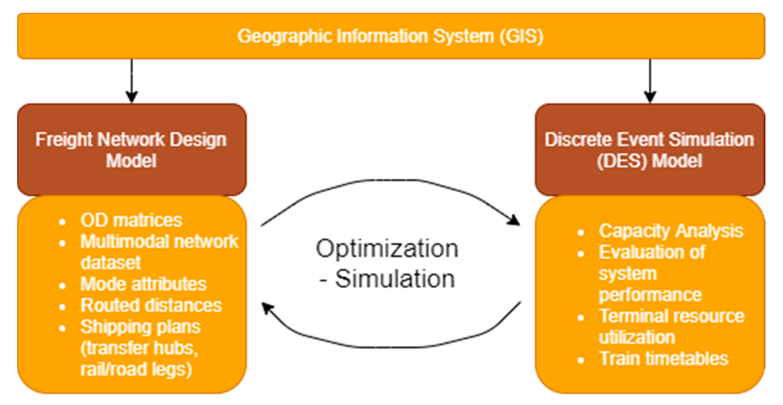
2.1. Sequential Optimization Simulation Framework

There are numerous combination possibilities with regard to the hierarchical structure and purpose of the simulation [38]. The hierarchical structure of the approach presented in this paper is based on a sequential optimization-simulation approach as outlined in Figure 1. The optimization side takes the form of a GIS-based network model. The network model allows analysts to generate optimal shipping plans for several commodity-specific origin–destination (OD) pairs, delivery routes, allocate transport modes to every leg of the transport chains, quantify traffic through the network, and select intermodal hubs. The counterpart comprises a GIS-based DES model. Simulation allows a step beyond the solution from the network analysis, evaluating different infrastructure arrangements to deliver satisfactory system performance in terms of shipping time, resource utilization, train frequency and queuing time at terminals. The method endorses a whole-system approach addressing traffic assignment, mode allocation, network planning, hub location, train scheduling, and terminal design.

The novelty of the method described in Figure 1 is in considering all these components together, as part of a strategic planning framework to assist the generation of a future concept for the freight system. Moreover, the interconnection between optimization and simulation provides the versatility needed to connect network and terminal planning perspectives, as the method contemplates geographic accessibility and terminal performance, allowing the streamlining of terminal location and logistics resources.

According to recent reviews on the simulation of intermodal freight transportation systems, the framework proposed in this paper falls under the category of sequential optimization—simulation approaches [38,39]. The optimization side is represented by a network design model that takes a set of OD matrices and multimodal network datasets as inputs. The solution delivered from the network model contains information on traffic through every arc of the network. Specifically, the model delivers shipping plans that are arranged into a database. The counterpart is based on a DES model that enhances the analytical solution provided in the optimization step. Agents within a GIS space interact with each other in response to shipping orders generated as discrete events. Shipping plans are based on the optimal paths queried from a database. The simulation accounts for truck and train trips, loading and unloading operations. The architecture of the simulation model allows analysts to set up different experiments, defined by the availability of resources, network configuration and agent attributes. The integrated model delivers the utilization of railyard tracks, train timetables, queue size at ports, and energy use for different scenarios. The following Section 2.1.1 and Section 2.1.2 provide more details on each module from the framework.

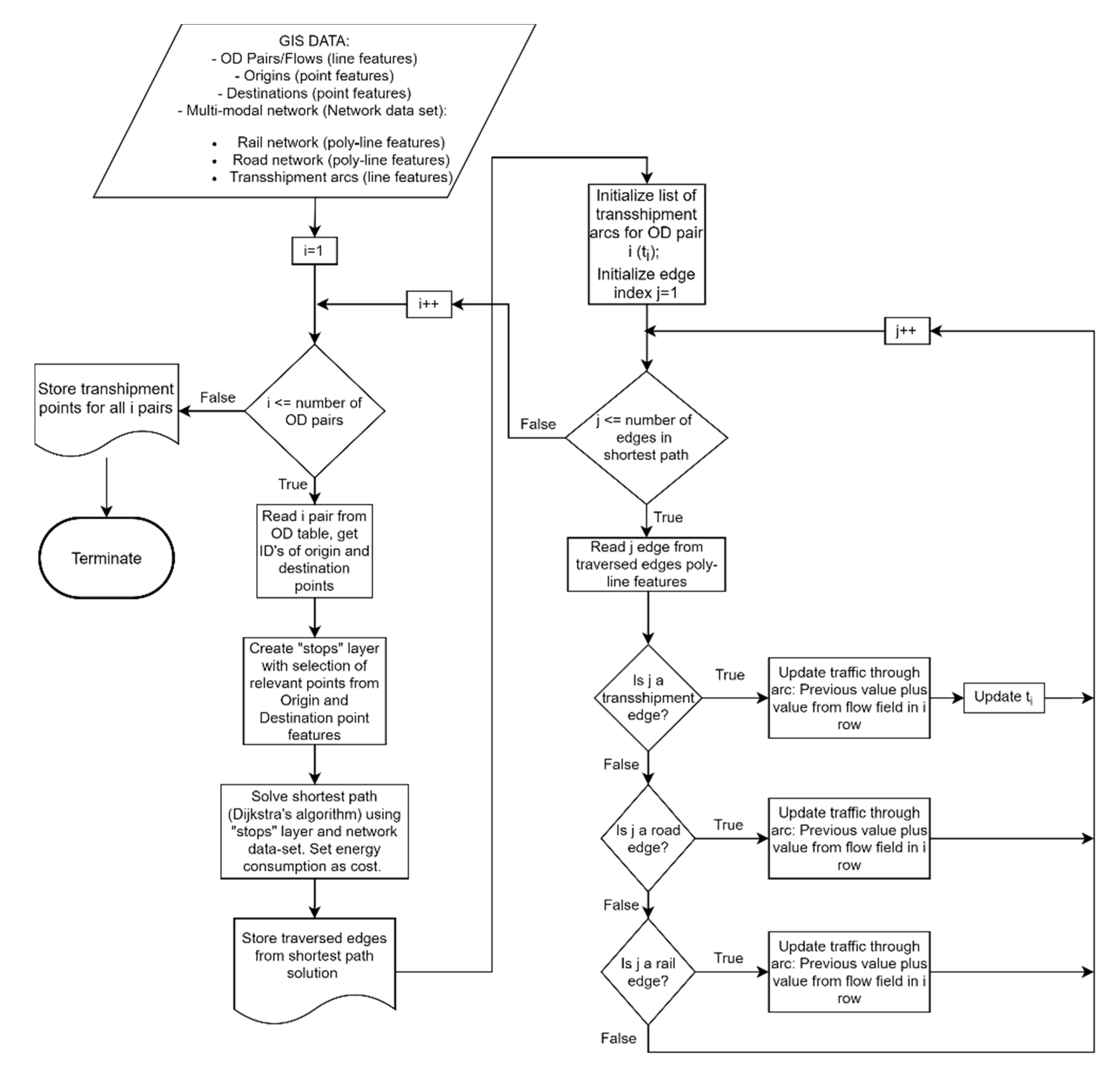
2.1.1. GIS-Based Network Model

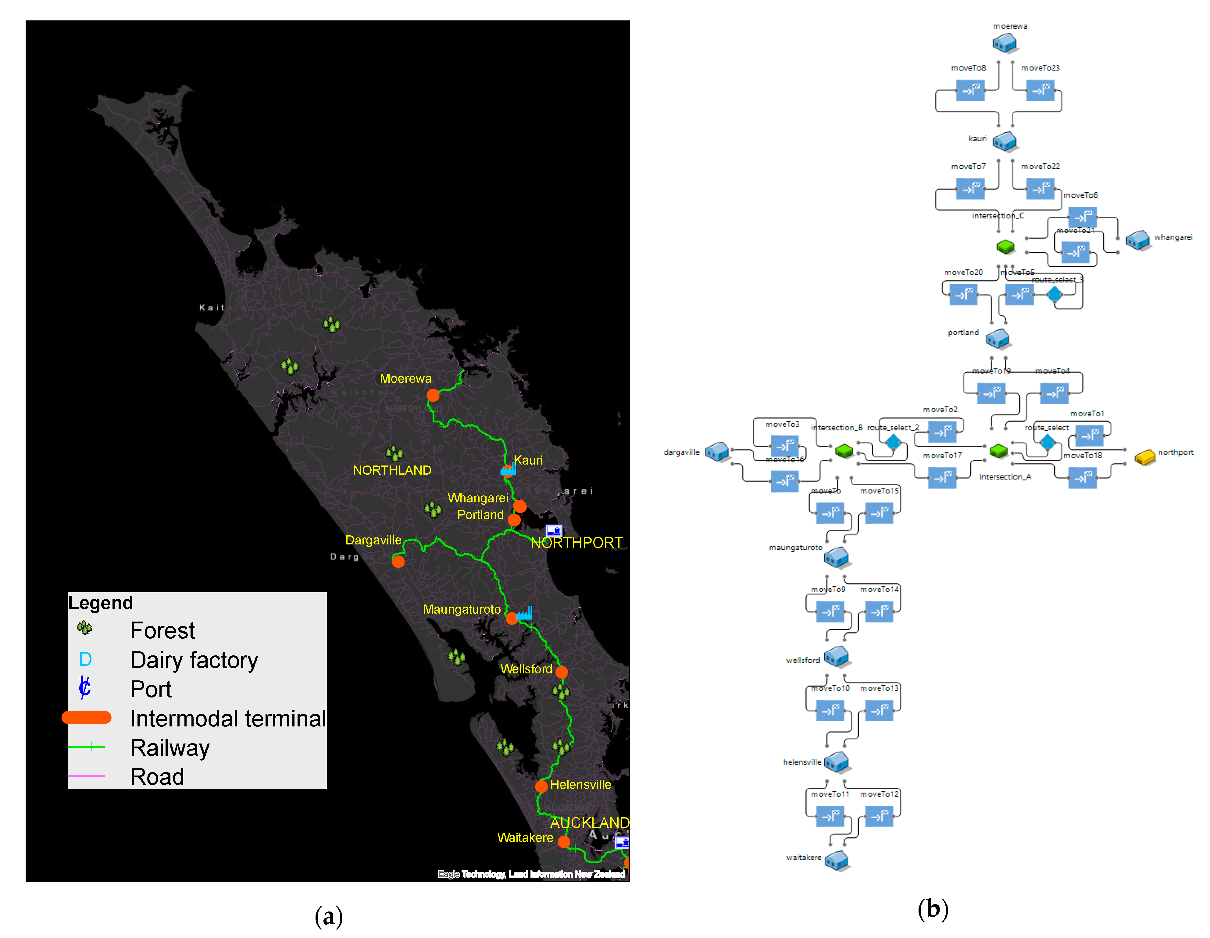
Figure 2 shows the algorithm for a network design model with an embedded shortest-path solver based on Dijkstra’s algorithm [45]. The network model takes a set of line feature classes (OD matrices), point feature classes (origins and destinations) and multimodal network datasets as inputs. Before actual model execution, a multimodal network dataset is constructed. During the building process, network elements are created, connectivity is established, and attributes are assigned to every type of link. Links are made up of roads, rail spurs and transshipment edges, with the corresponding distance, time and energy use attributes associated with each transportation mode. Nodes are made up of ports, terminals, factories, warehouses and material-extraction facilities.

For every OD pair, Dijkstra’s shortest path is executed using either energy use or travel time as cost attributes. Time was estimated to be a function of routed distance and mode-specific cruise speeds. The links (road, rail and transshipment arcs) that integrate every solution or shortest route are assigned the corresponding traffic volumes. The model output is integrated by three line feature classes representing road, rail and transshipment edges respectively. Every edge in the solution has a traffic attribute associated with it, representing annual flow under the optimal scenario. Moreover, for every OD pair, a shipping plan is generated and recorded, containing information on origins, destinations, mode allocation and transfer nodes. The model output also allows the identification of train stations that can become intermodal hubs and road arcs with enough traffic to justify spur extensions from the railway network. Train routes and frequencies are arranged based upon the traffic estimates, and tested during the simulation. The algorithm was coded in Python 2, using network analysis functionality from the arcpy library.

2.1.2. Discrete Event Simulation Model

The model was created in the simulation platform Anylogic 8.5.2. Anylogic was particularly useful, as it integrates GIS maps and allows researchers to build networks from shapefiles. The software offers a multimethod environment that combines discrete event agent-based modeling (ABM) and system dynamics methods. Moreover, it has specific libraries that allow the simulation and visualization of precise operations of railway systems, manufacturing and warehouse workflows. This model is concerned with a long-term vision that fully embraces multimodality as a strategic pathway to support national commitments toward climate change mitigation. Accordingly, the network model described in the previous section delivers a deterministic solution and the simulation counterpart allows users to gauge the system configuration and capacity required, through the evaluation of different experimental setups.

The simulation module contemplates transport agents (i.e., trains, trucks), terminal agents (i.e., intermodal terminals and ports) and production agents (i.e., forests, factories) interacting within a GIS space in response to shipping orders defined through rates. Orders are sourced from relevant facilities (i.e., factories, ports). Rate values are obtained from a database through queries requesting information on the origin and destination of the shipment and on the type of commodity to be transported. Once a shipping order is sourced, a transportation service is arranged. Depending on the location of the facility and its accessibility to the railway network, three services are considered: truck-only, intermodal and rail-only services. Shipping plans generally involve intermodal trips, based on optimal paths queried from a database. The assignment of an intermodal hub is carried out through a query, which retrieves information on the location of transshipment points. By default, Anylogic offers routing functionality, allowing agents to move through road and railway networks based on data extracted from OpenStreetMap servers.

Loading and unloading operations take place at intermodal terminals, and their performance is contingent on the operation time and availability of resources (cranes and forklifts). Operations simulated at terminals are limited to the logistics side, capturing the interactions between trucks, trains and loading equipment, and subsequent repercussions on the broad freight system. The scope of the model does not contemplate yard and storage planning as is the case with other simulation models that focus solely on terminal operations [46]. Daily train services are simulated, the routes and frequencies are derived from the traffic estimates of the optimization module. The model allows users to assess used railway capacity, that is, it reflects potential traffic and varies with changes in infrastructure and operating conditions [47]. In particular, railway capacity is ascertained from upgraded double-track network segments, train speed, and terminal performance (stop times).

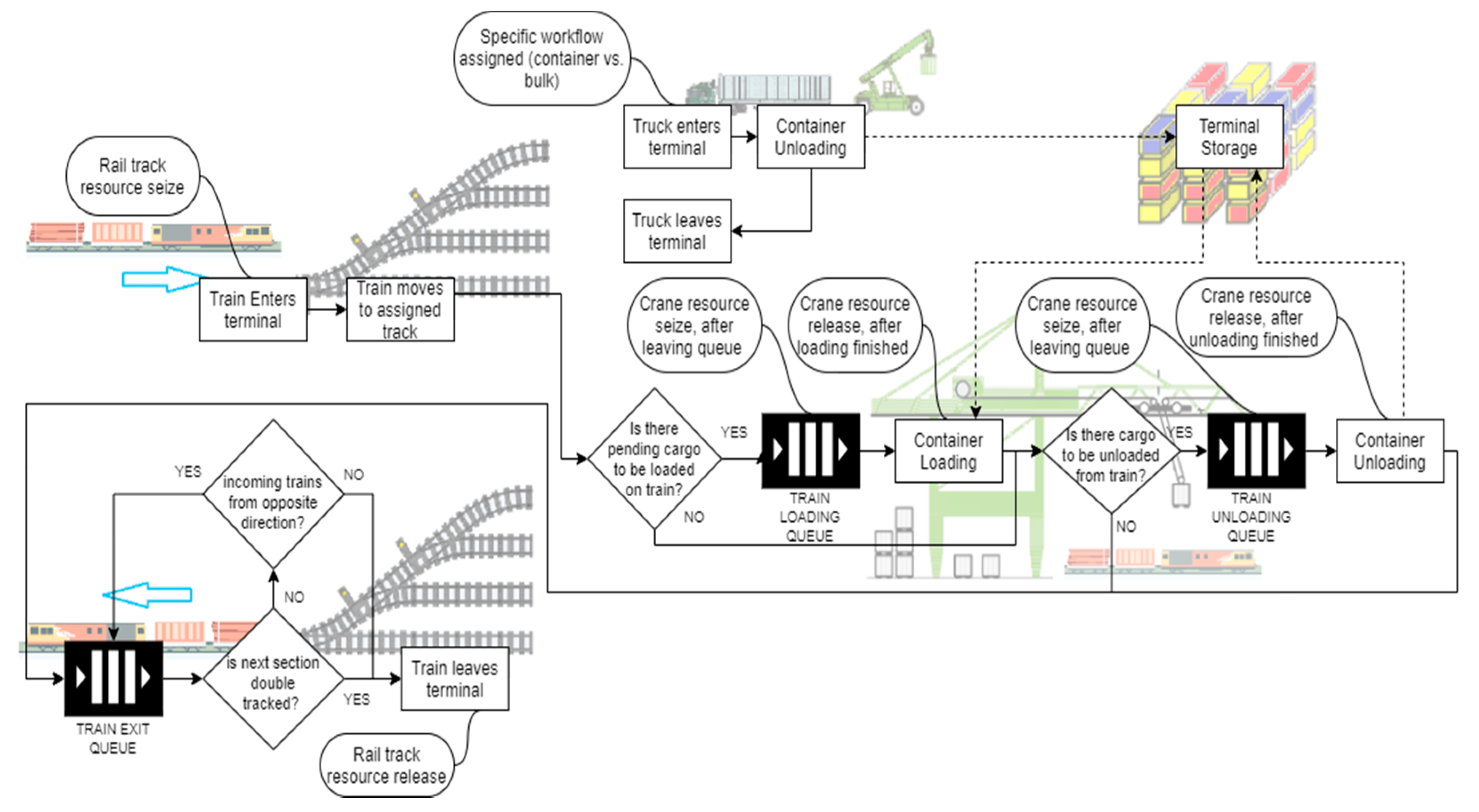
Figure 3 presents a general workflow for a terminal agent. The workflow connects a network of service nodes consisting of queue and server blocks [48]. A train enters a terminal and is assigned a track element from a collection of tracks representing a railyard. The number of tracks at each railyard is exaggerated, as the goal of the simulation is to precisely determine railyard utilization upon the model execution, and to fine-tune the railyard arrangement in order to deliver the number of tracks needed to guarantee the continuous operation of the system.

If cargo needs to be unloaded, a crane is requisitioned from a pool of crane resources. Unloading times are simulated through delay blocks. Cargo is unloaded from the train and placed on a storage queue, where it can be picked up by a truck and delivered to its final destination. Once train unloading is over, the crane resource is released back to the pool and the train is ready to pick up any pending cargo from a second storage queue. Train loading proceeds in a similar manner as before, that is, a crane is requisitioned during train loading. After loading and unloading operations, the train enters a queue. In case there is a train that is not required to drop off or pick up a load, it is also possible for it to directly enter the exit queue. In this situation, auxiliary variables and functions are used to monitor the conditions of trains that enter the railyard, and to manage their movement. Movement between the railyard and the exit track is also modeled with the seize-release approach. The exit track is established as a resource to ensure that only one train exits at a time. A holding block is also considered before a train exits, which is activated when trains are approaching the terminal from a direction opposite to that of the exiting train. For some terminal agents, the actual operations can be more complex and there will be a workflow similar to that of Figure 3 for every line. When a train enters a terminal, a specific workflow is applied, similar to that shown in Figure 3, where every train is monitored and assigned specific loading or unloading instructions. Terminals are programmed to allocate distinct workflows, depending on the type of cargo handled within their premises. 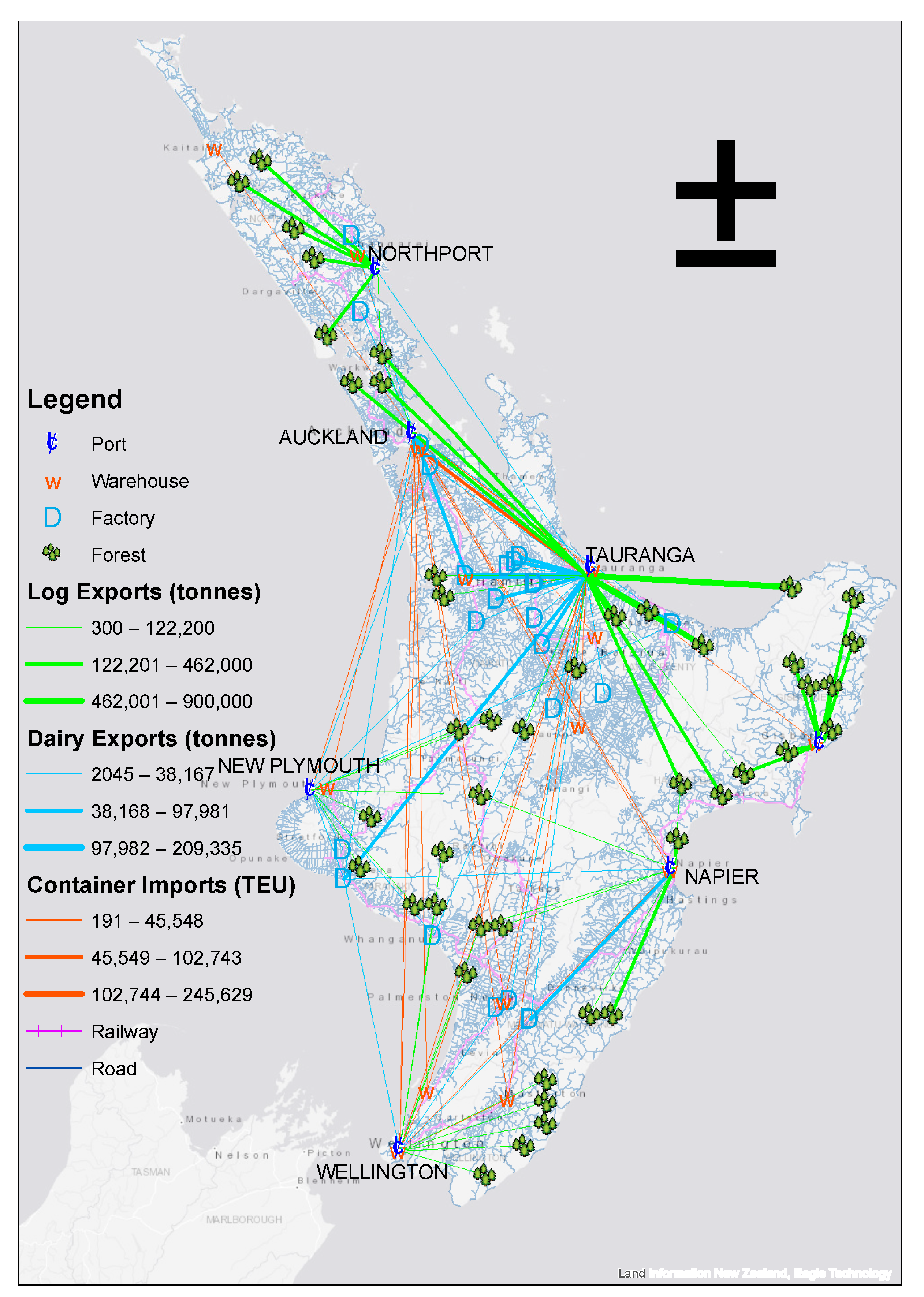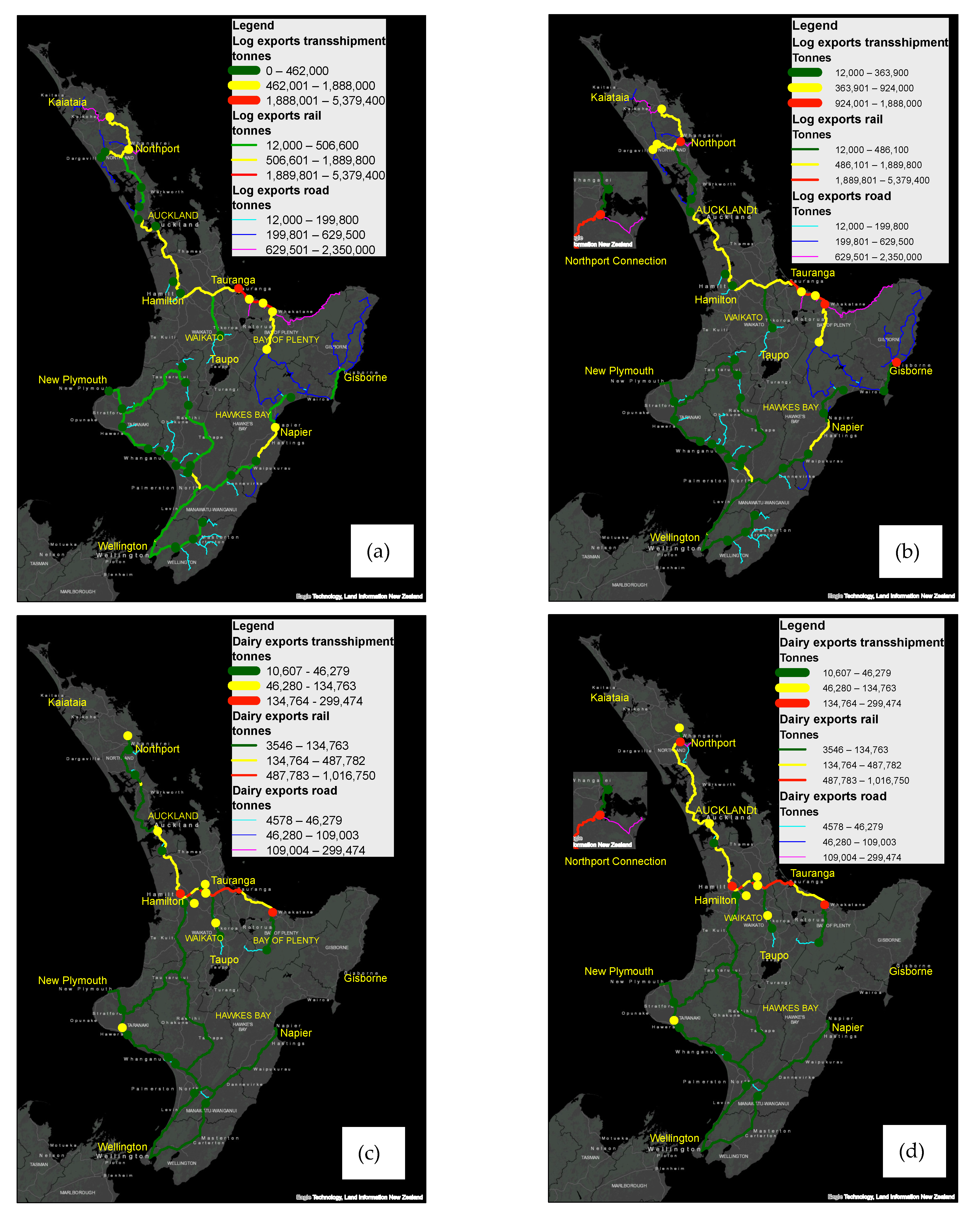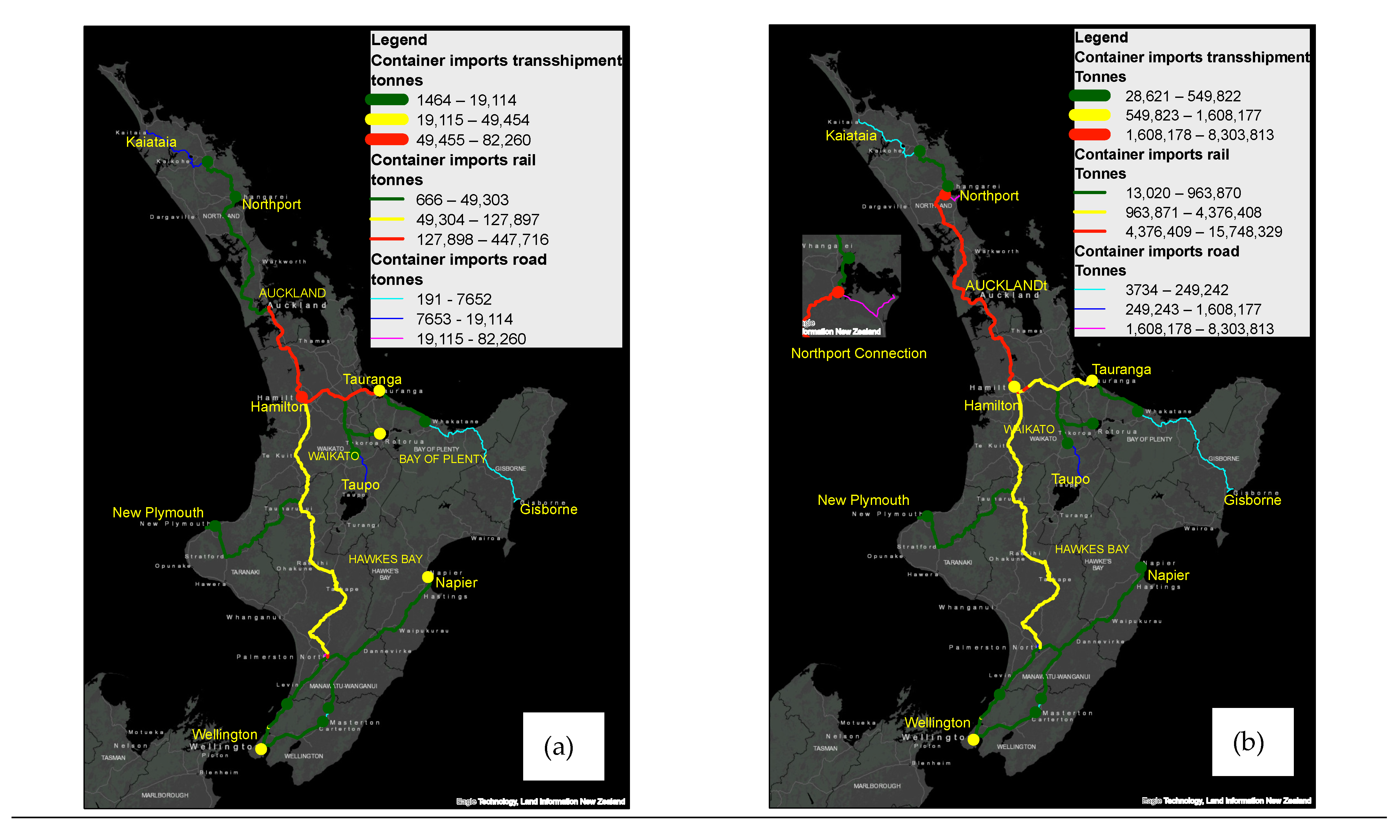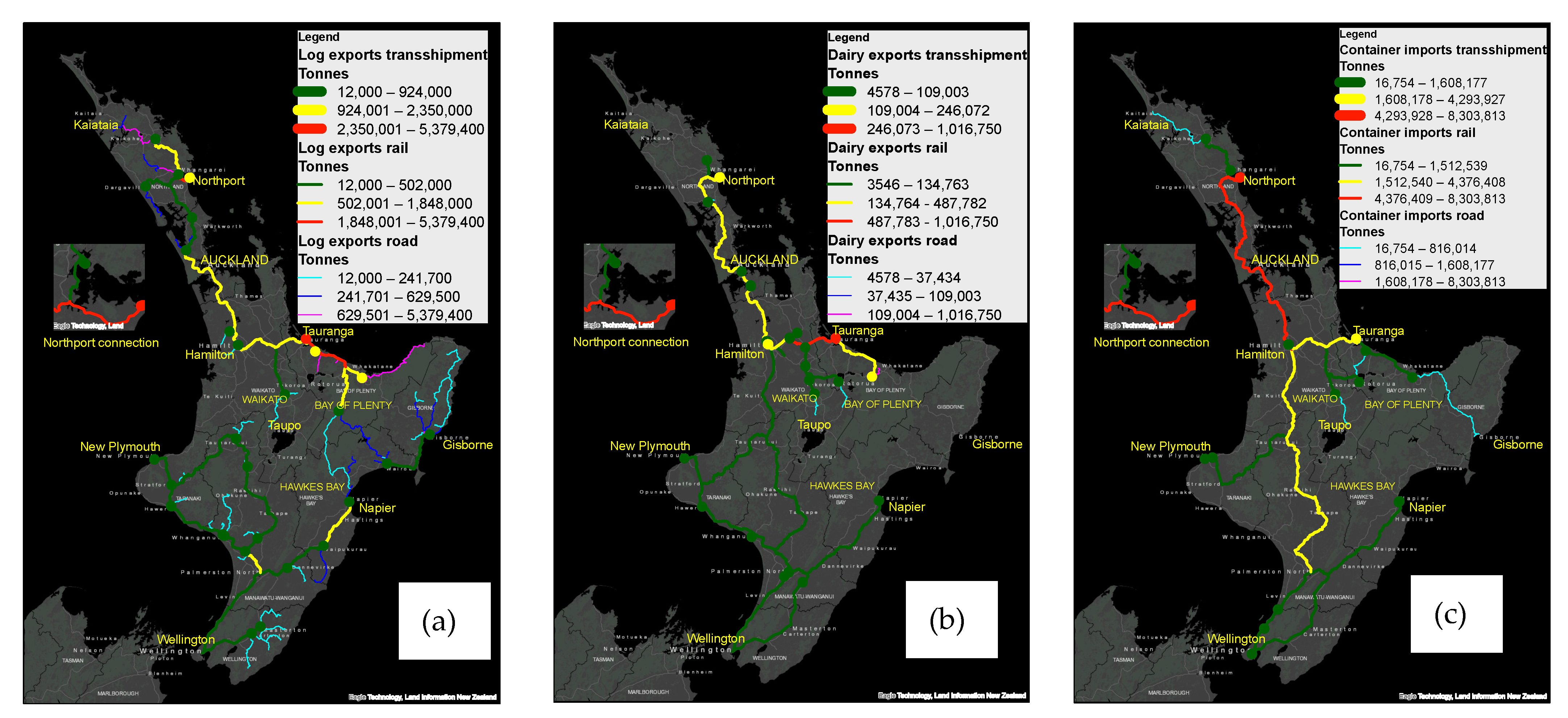For instance, Figure 4 presents OD pairs for bulk and containerized freight moved within the North Island of New Zealand; this information is provided as Supplementary Materials. The programmatic allocation of workflows was enhanced through the implementation of Java interfaces. Interfaces allow users to execute generic functions on different terminals. For instance, a take function instructs a terminal to allow a truck agent to enter and unload a shipment. The interpretation of the function depends on the type of terminal, as there are specific workflows for different commodity types. Moreover, different lines will serve different purposes, including the following cases: trains passing through the terminal on the way to their final destination, trains picking up or dropping off cargo on their way to their final destination, trains that have arrived at their final destination to be unloaded, or trains originating at the terminal and loaded with cargo while waiting for departure. The workflow in Figure 3 provides an overall representation of the model’s logic and can be adapted to specific cases.

3. Model Implementation in the North Island of New Zealand

This section presents a closer look at the method displayed in Figure 1. New Zealand’s North Island is used to deliver a proof of concept. The commodities used to carry out the method are timber and dairy products for export. Containerized freight flows are dominated by import goods destined for the largest city, Auckland. The Northland region was denuded of native bush, and pine plantations were planted more than 40 years ago. The plantations supply logs for local MDF board manufacture and for export as raw logs. The plantations are being replanted as they are clear-cut harvested. While this is not ecologically ideal, the current system can be expected to be supplying some raw log exports into the next century. Intensive dairy production has grown over the past decade, with the main export being dried milk powder. The path-break concept modeling will use the same level of dairy freight as today. However, given the deleterious impacts on water and methane emissions, the path-break concept would actually require much less dairy, and a more diverse mix of products being exported, assuming the same volumes. Government reports continue to estimate growth in import freight into the distant future. Given the forward-operating environment restriction on fossil fuel production, we will use the same level of freight flows as today for the path-break concept.

3.1. Data Sources

Figure 4 gives a representation of the main model input, a set of line-feature classes representing export (dairy, logs) and import (general containerized freight) flows, in tonnes and twenty-foot equivalent units (TEU), within the North Island. Every row of the corresponding attribute tables contains data on a specific OD pair, including identification strings for origins and destinations, and annual flow between them. Flows were derived from a programmatic application of linear programming (LP), iterative proportional fitting procedure (IPFP) and calibration of spatial interaction models; more details on the method are provided in [49]. The geographic coordinates of the nodes involved were extracted through a Google Places API. The process was iterative; queries were composed using elements from lists of city and region names in New Zealand and case-specific keywords including “ports”, “dairy factories” and “warehouses”. The latter key term was also accompanied by the names of major logistic and transport companies in New Zealand.

Figure 4 shows that Ports of Auckland (POA) is currently a strategic gateway for overseas imports. It is through POA that containers enter New Zealand and are subsequently delivered to regions across the country. In the case of log exports, it was assumed that logs are mostly harvested from exotic forests. Representative forest locations were obtained from the New Zealand land cover database (LCDB) [50]. The multimodal network addressed in Section 2.1.1 is made up of roads, rail spurs and transshipment points, with corresponding distance, time and energy use attributes. For rail and road edges, time was estimated to be a function of routed distance, given average speeds of 30 km/h and 70 km/h, respectively. Transshipment time was assumed to be fixed, given a value of 5 min per tonne transferred. Energy use was also estimated as a function of routed distances. Energy intensities were obtained from the Lipasto database, assuming a partially loaded semi-trailer combination for road transport (0.74 MJ/tkm) and a diesel-driven container train for rail transportation (0.24 MJ/tkm) [51]. Energy demand for transshipment operations was assumed to be fixed, with a value of 1.58 MJ per tonne transferred, which was derived from previous studies assuming an average weight of 12.7 tonnes per TEU [23,24]. Road links are based on the NZ Road Centerlines file, available to the public through Land Information New Zealand (LINZ) [52]. Railway links and stations were obtained through KiwiRail’s open-source GIS data platform [53]. Train stations used in the network analysis have been verified to have more than one track, and are considered as candidates for intermodal hub selection. Aside from the geographic representation of the network, Figure 4 also shows a contrast between import and export volumes for POA and Port of Tauranga (POT), respectively. Moreover, Northport appears as a strategic location for log exports.

3.2. Scenario Definition

According to a recent report published by the Ministry of Transport [54], the future operation of POA will be increasingly constrained in its economic or environmental viability, due to landside infrastructure friction. The report also recommends that Northport should be developed to take over much or all of Auckland’s existing and projected future freight business [54]. In line with these recommendations, the network model is executed under different scenarios. With regard to the pattern of flows, two cases were considered, business as usual (BAU) and full shift (FS) of the Ports of Auckland freight to Northport. In the case of BAU, the current pattern of flows is maintained and POA remains operational. In the case of FS, all activity is shifted from POA to Northland. The current railway network does not have a connection to Northport. The model is executed with (WC) and without a railway connection (NC) to Northport. Finally, the execution of the network model considers two attributes for optimization, energy use (E) and travel time (T). The results in Section 4.1 cover a range of six scenarios that are based on a combination of the aforementioned interventions. In summary, the six scenarios are:

• BAU-NC-E—BAU freight landings at Ports of Auckland (POA) with energy optimization
• BAU-NC-T—BAU freight landings at Ports of Auckland (POA) with time optimization
• FS-NC-E—Full shift to Northport (NP) with optimization on energy
• FS-NC-T—Full shift to Northport (NP) with optimization on time
• FS-WC-E—Full shift to Northport (NP) with rail connection (WC); optimization on energy
• FS-WC-T—Full shift to Northport (NP) with rail connection (WC); optimization on time

3.3. Performance Indicators and Cost Estimation

Network capacity and resources are streamlined through the execution of different simulation experiments. Each experiment accounts for different setups and parameters, including train speed, number of wagons per train, number of cranes and forklifts at each terminal, and single or double-tracking sections.

For every experiment, the performance is monitored through resource utilization rates, the number of sidings/tracks used at each terminal, and train timetables. Performance of the system was monitored during each setup, and parameters and resources were adjusted to improve utilization rates, and to ensure that each train performed a round-trip within a period of one day and to guarantee balanced inventories at terminals. Cost estimation is based on the parameters defined for every experiment (see Appendix B for costing categories). Terminal areas were calculated based on the number of loading units exchanged at each terminal, and reference values were based on figures reported in [55].

4. Results

The following sections summarize the main results and findings. Section 4.1 addresses the main findings from the execution of the network design model. Section 4.2 covers the results from the execution of the counterpart simulation.

4.1. Network Design Model Results

Energy use and average travel times for each scenario are reported in Figure 5. Scenarios that show more reliance on road shipping were associated with time-based optimization (BAU-NC-T, FS-NC-T and FS-WC-T), resulting in shorter travel times. On average, scenarios where energy use was optimized were associated with travel times 170% higher than those of time-based optimization scenarios. In contrast, scenarios where travel time was optimized have 86% more energy demand than scenarios based on energy use optimization. Overall, a full shift to Northport would entail longer distances between the port and final destinations, and consequently would lead to higher energy demand. This aspect is reflected in Figure 5, as scenarios that include a full shift to Northport (FS) have a higher total energy consumption than the business-as-usual cases (BAU) where POA is fully operational. If the shift to Northport becomes effective, it is evident that there would be an urgent need to develop an infrastructure that can mitigate the potential increase in energy demand. Figure 5 also provides insights into the plausible impacts of a full shift. If there are no interventions regarding infrastructure, and trucking remains the dominant mode of transportation, energy demand could increase by 86% in the worst-case scenario (FS-NC-T).

Figure 6 shows total emissions for all scenarios. Overall, emissions are proportional to energy demand, as expected. For the Full Shift to Northport (FS) and optimization on time (T) scenarios, trucking remains the dominant mode, and GHG emissions can reach up to 260 thousand tonnes of CO₂eq. In contrast, the best-case scenario (FS-WC-E) shows a 47% reduction in gross emissions, which is feasible but is still not enough to meet the national 2050 target of a 70% reduction. Further reductions could be achieved either through a reduction in transport activity (tkm), through the relocation of factories and warehouses, and by electrification of the rail freight, given New Zealand’s renewable energy capacity.

The main motivations behind the move to Northport are congestion within the city of Auckland, which drives inefficiencies throughout the local supply chains, and the redevelopment of the waterfront in the central business district. It is expected that a shift to Northport will alleviate current congestion levels, and will also enhance land use transformation, potentially allowing port land to achieve higher returns than the current port’s dividends [56].

Figure 7 shows traffic assignment throughout the network for exports where energy was used as a cost attribute. The relocation of POA relieves some of the traffic around Auckland but increases congestion levels on the links connecting to Northport. For the current pattern of flows (BAU), traffic is concentrated across the regions of Auckland, Waikato, and the Bay of Plenty. Hamilton appears as a key location, as it provides a strategic connection point between POA and POT. Moreover, there are road segments with significant traffic where railway tracks could be deployed and take advantage of economies of scale. This is the case with the road segments connecting to Kaitaia in the Northland Region and Taupo in the Waikato Region. Despite the railway connection to Gisborne, the port seems to require an alternative and more direct route to the Bay of Plenty Region.

Given a relocation of the port, Figure 8 shows that the railway segment north of POA can potentially become a bottleneck in the movement of container imports. The capacity of this section can be enhanced through upgrades in railway infrastructure, double-tracking, and the deployment of intermodal railyards. The traffic estimates from the network model output allow identification of the service lines and train frequencies that would be required to meet the freight demand within the region. The train frequencies are confirmed during the simulation step, as the operational capacity of the railway system also depends on the performance of loading and unloading operations at the terminals.

Figure 9 shows the results when including a direct rail connection to Northport. In the long run, the rail route can lower energy demand even further and reduce road congestion in areas in the vicinity of the port. The traffic estimates shown in Figure 9 can be useful when assessing network capacity, as the geographic and topological layout of the simulation model is based upon these estimates. The assessment also allows the identification of the most suitable locations for the development of intermodal hubs. According to the results, 46 out of 109 hub candidates were selected in the best-case scenario (FS-WC-E). The model provides details on the type and volume of freight handled at each hub, hence this information was used during the simulation step to assess the resources that would be required, depending on the type of commodities to be handled at the terminals.

4.2. Capacity Assessment for the Best-Case Scenario

The lowest energy, lowest cost scenario is a full shift in freight activity from Auckland to Northport, with a direct railway connection to the port and shipment routes based on energy use optimization (FS-WC-E). The connecting link between the network analysis and simulation models is a database with optimal shipping plans corresponding to a full move to Northport. The network layout for the simulation accounts for the addition of intermodal terminals. Figure 10 provides the logical representation of the railway network, which corresponds to the upper part of the North Island. The workflow uses Anylogic’s symbology and has embedded functions and auxiliary variables that allow researchers to coordinate train movements within the network. For instance, for every section that is covered between terminals, there is an auxiliary Boolean parameter that, when set to True, blocks the movement of trains in opposite directions when the section is single-tracked.

Nine intermodal terminals were considered from North to South; these are Moerewa, Kauri, Whangarei, Portland, Northport, Dargaville, Maungaturoto, Wellsford, Helensville and Waitakere. They have similar functionality because intermodal operations are allowed on all of them. However, they do not necessarily provide the same services, as some of them only handle a specific type of commodity or serve specific train lines. The traffic assessment represented in Figure 9 allowed us to identify six train services. Line 1 is dedicated to carrying imported containers to Waitakere, which is an inland terminal located on the northern outskirts of Auckland. Trains returning from Waitakere pick up export logs from Helensville and Wellsford, and dairy exports from Maungaturoto. Line 2 is fully dedicated to exporting logs from Dargaville. Lines 3 and 5 are dedicated to carrying imported containers to Moerewa and Whangarei, respectively. On the way back, lines 3 and 5 pick up logs and dairy exports from stations located on the journey to Northport. Line 4 is fully dedicated to exporting logs from Portland. Line 6 picks up dairy exports from Kauri and, on the way back, picks up export logs from intermediate stations.

The model time was set to 50,000 min, and in each experiment, several parameters were tuned, including train speed, number of forklifts, number of cranes, number of wagons per train, and segments with double tracks. Crane and forklift operation times were assumed to remain constant throughout all experiments, with values of 1.3 min and 1.5 min, respectively. These values were timed from operations at local ports, and are in agreement with those values reported in the literature [46].

Table 1. Setup and terminal resource utilization for different simulation experiments.

Description	Exp. 1	Exp. 2	Exp. 3	Exp. 4	Exp. 5	Exp. 6
Train speed (km/h)	35	35	35	50	35	35
Number of forklifts (Utilization %)
Moerewa	5 (2.8%)	3 (4.5%)	3 (4.6%)	3 (4.7%)	3 (4.9%)	3 (4.7%)
Northport	10 (3.8%)	8 (4.7%)	8 (4.8%)	8 (4.8%)	8 (5.1%)	8 (5.0%)
Portland	10 (1.9%)	3 (4.6%)	3 (4.7%)	3 (4.4%)	3 (5.5%)	3 (5.3%)
Dargaville	5 (2.0%)	3 (3.3%)	3 (3.3%)	3 (3.3%)	3 (3.8%)	3 (3.7%)
Wellsford	5 (0.01%)	1 (0.03%)	1 (0.02%)	1 (0.05%)	1 (0.03%)	1 (0.08%)
Helensville	5 (1.6%)	4 (2.1%)	4 (2.1%)	4 (1.9%)	4 (1.9%)	4 (1.9%)
Number of Cranes (Utilization %)
Moerewa	5 (1.9%)	3 (2.5%)	3 (2.5%)	3 (2.5%)	3 (2.3%)	3 (2.4%)
Kauri	5 (0.09%)	1 (0.4%)	1 (0.4%)	1 (0.6%)	1 (0.5%)	1 (0.5%)
Whangarei	5 (0.7%)	1 (3.6%)	1 (3.4%)	1 (3.4%)	1 (3.8%)	1 (3.8%)
Northport	10 (12.4%)	10 (13.0%)	10 (13.5%)	10 (13.4%)	10 (11.5%)	10 (10.5%)
Maungaturoto	5 (0.04%)	1 (0.1%)	1 (0.2%)	1 (0.2%)	1 (0.2%)	1 (0.1%)
Waitakere	10 (10.8%)	10 (11.3%)	10 (11.2%)	10 (11.1%)	10 (12.3%)	10 (12.3%)
Wagons per train	20	20	20	20	25	25
Double-track segments	All single track	All single track	Wellsford– Waitakere	Wellsford– Waitakere	Wellsford– Waitakere	All single track
Total number of railyard tracks	90	91	85	101	84	89

summarizes the setup and resource utilization in each experiment. The overall aim was to evaluate trade-offs amongst parameters on each test, and demonstrate how the model can be used to streamline the arrangement of the conceptual design. The first setup is based on a predefined number of resources at different terminals, and on single-tracked sections throughout the network. During Experiment 2, the number of resources is reduced to improve utilization rates while maintaining smooth operations throughout the network. In this study, utilization is defined as the fraction of time that units were busy. There are terminals that, despite having reduced resources, still show signs of resource underutilization, yet crane and forklift numbers are maintained throughout the remaining experiments, as further reductions are non-feasible. In Experiment 3, double-tracking is implemented in the sections assessed between Wellsford and Waitakere. In this case, the major benefit of double-tracking is the reduction of round-trip travel times.

Figure 11 provides a representation for train timetables corresponding to line 1, which runs from Northport to Waitakere. Comparing Experiments 1 and 3, it is evident that double-tracking cuts round-trip times by 500 min. In Experiment 4, train speeds were increased from 35 km/h to 50 km/h, leading to a further 500-min reduction in round-trip time. This reduction in travel time can be exploited, as more trains could be added in case they were needed. Moreover, these additional time savings can enhance additional clearance for loading/unloading operations at terminals. The timetable for Experiment 6 shows that the addition of 5 wagons per train slightly increases round-trip times if compared to the timetables from Experiment 1. Nevertheless, in Experiment 6 all trains managed to do a round-trip before the end of the day shift, despite low train speeds (i.e., cruise speed) and single tracks throughout the network. It is worth mentioning that the values reported refer to cruise speeds, as the software allowed us to model train acceleration and deceleration within terminals, and speeds vary accordingly.

Table 1 shows that interventions associated with Experiments 2, 3 and 4 do not cause a major impact on resource utilization. Experiments 5 and 6 are the exception; adding additional wagons reduces queues, hence requiring additional resource operation that leads to higher utilization rates in some cases. Figure 12 contrasts the queue levels for Experiments 2 and 6. An accumulative trend of queue levels was observed during the execution of Experiment 2. In Experiment 3, the implementation of double-tracking partially improved the cumulative effect at some terminals. However, long queues were showing signs of accumulation at Dargaville. The addition of extra wagons under Experiments 5 and 6 led to relief in timber volumes from the terminal at Dargaville. Furthermore, additional wagon numbers allowed us to reduce queues in other dairy-handling terminals, leading to additional benefits that can potentially represent cost savings in terms of storage space.

Table 1 includes the total number of railyard tracks required for each experiment. Comparing the number of tracks for Experiments 2 and 3 illustrates the benefit that double-tracking has on railyard size: the number of tracks or sidings is reduced by 6. The increase in train speed affects railyard size as it shifts track numbers from 85 in Experiment 3, to 101 in Experiment 4. An upgrade in train speed (Experiment 4) results in additional track requirements from terminals throughout the network. In general, there are different trade-offs at stake, involving upgrades in rolling stock, railway network and terminal tracks.

A cost analysis was needed in order to identify the most effective interventions. Figure 13 presents the results of the cost analysis. In the worst-case scenario (Experiment 4), the costs can reach a total of 1.2 billion NZD, mainly because a major upgrade of the railway network could allow the movement of faster trains. An investment of such magnitude could be considered if volumes from other commodities led to the adoption of additional train services. An increment in train services could also be enhanced through double-tracking specific sections. If double-tracking was the desired pathway, the setup of Experiment 5 would be the most suitable option, as it not only allows for a coordinated movement of daily train services but also manages to avoid the steady increase in inventory levels at terminals. The results suggest that Experiment 6, with a corresponding total cost of 476 million NZD, would be the most cost-effective setup because it enhances a continuous operation of train services without the need for costly network upgrades and is associated with low inventory levels at terminals. The analysis was based on the transport demand associated with three particular sectors, meaning that the movement of additional freight volumes would require the implementation of double-tracking in order to allow the adoption of additional train services. However, one of the sectors considered is forestry, and according to past trends and recent projections, timber volumes fluctuate over time. It is expected that within the next two decades, activity associated with log transportation will decrease, but will then increase as current plantings mature.

Despite the reduced number of handling resources at Kauri in the north, and Maungaturoto and Wellsford in the south, the utilization rates were extremely low. A further set of simulation experiments could consider fewer terminals, where Moerewa could absorb the activity from Kauri, and Maungaturoto and Wellsford could fuse at an intermediate location. The reduction of terminals would also need to be tested through simulation, as fewer terminals imply a reduction in land costs but also limit the frequency of train services in the network.

5. Discussion and Conclusions

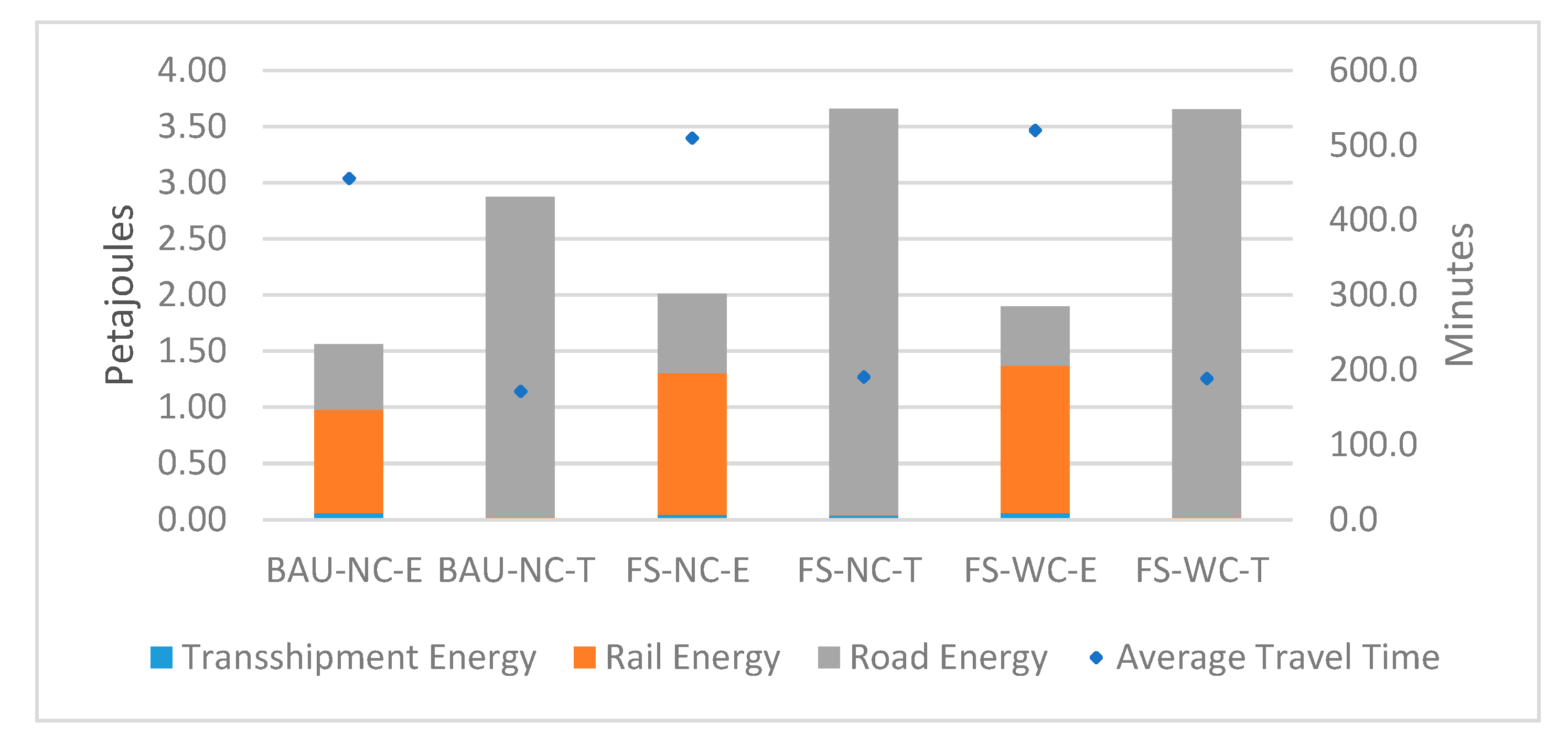
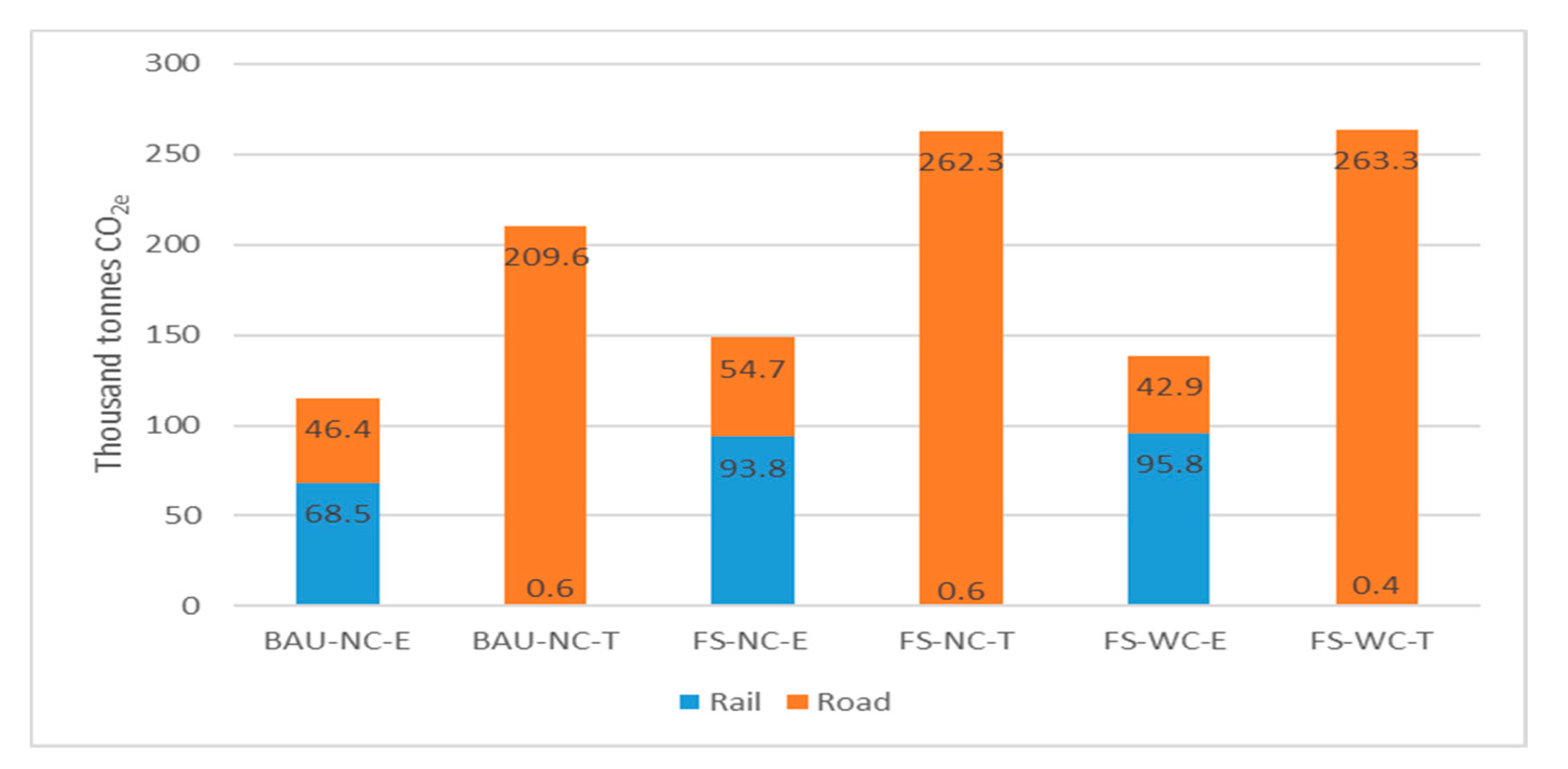
New Zealand has counted on its railway services for over 150 years. Despite the long history of rail in New Zealand, the share of TKMs has been decreasing and is currently bordering 10%, freight trains are still running at relatively low speeds, and network infrastructure has been left to deteriorate as needed upgrades have been postponed or omitted. Despite its present condition, the results from this study suggest that the current railway infrastructure can serve a much higher share of the freight task, given that effective access to the network is provided. Specifically, the availability of intermodal infrastructure guarantees that all stakeholders involved, including shippers and producers, will be able to engage in shipping in the Next Century concept freight network.

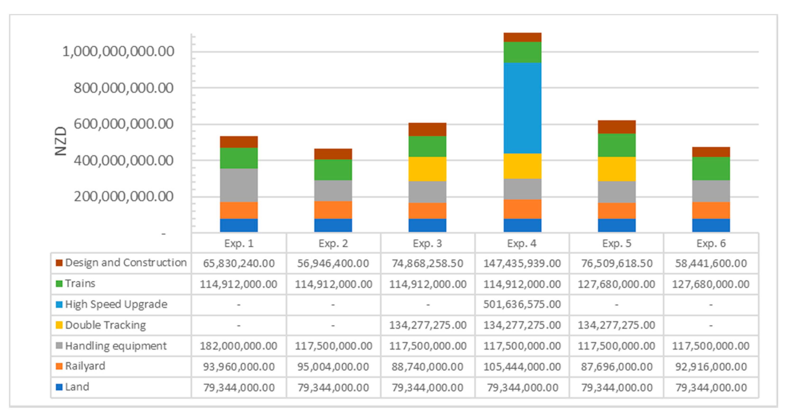
Simulation results were complemented by a costing assessment to identify the most cost-effective setup. The results suggest that costly interventions are not necessarily aligned with the most effective way forward. The setup associated with Experiment 6 did not consider double-tracking or a track upgrade to improve train speed, and yet can potentially foster a drastic reduction of emissions through the adoption of key intermodal terminals. Accordingly, future investments should prioritize the development of intermodal hubs that can improve supply chain accessibility to railway transportation. It is worth clarifying that other line items, like traffic control systems, signals, crossing gates, storing equipment, and handling software were not included in the costing analysis. These items could be accounted for as part of the basic and detailed design stages, where simulation can also take a protagonist role.

New Zealand was used for the proof of concept, and there are elements that will be typical in other geographical contexts, particularly ongoing regional and international trade and the supporting infrastructure, including road and railway networks, terminals and ports. All these elements have been characterized in this study. The interconnection between optimization and simulation provides the versatility needed to connect network and terminal planning perspectives. The framework not only allows analysts to engineer a future concept of the network layout but also interrogates the operational capacity needed to withstand a substantial modal shift to rail in response to national carbon mitigation strategies. These advantages are not only relevant in New Zealand, but also can potentially be used to assist the development of energy and transport policy in other countries and regions. Moreover, countries that currently lack a railway infrastructure can still replicate some features from this study, as the framework can be used to distinguish freight corridors with significant traffic levels that can potentially be considered for the development of a railway network layout.

State-of-the-art agent-based freight models embrace a communication framework that supports negotiation and decision-making amongst cognitive agents. The framework presented in this study accounts for the heterogeneity of actors in the supply chain, although the approach leaned toward a pure discrete event nature. There was no negotiation amongst agents, they only reacted to the presence of other agents, scheduled orders and events. Furthermore, recent models reported in the literature have studied agent behavior within a transportation market. In these models, agent behavior has been calibrated by surveys that reflect the status quo, which prioritizes cost and transit time over environmental considerations. Accordingly, the method presented in this study deviates from these state-of-the-art approaches, as agents are restricted to following optimal shipping plans, minimizing the use of energy resources.

The adoption of DES was relevant because the interaction of agents is not static; freight operations take place within a dynamic environment, where different events are simultaneously taking place at different levels of the system. The simulation allowed the capture of the synergy between train and terminal operations. From the network operator perspective, the movement of trains depended on the network layout (distance between stations and single- vs. double-tracking) and on cruise speed. From the terminal operator side, train arrivals and departures were contingent upon the performance of handling resources at ports and terminals. In some cases, the low utilization of handling equipment at terminals may justify the execution of further iterations based on alternative arrangements. As a complementary component, simulation allowed utilization to be tracked and to streamline a concept that can fulfill the expectations of stakeholders involved during the planning process.

It is difficult, if not impossible, to accurately predict long-term freight transport demand. Current transport demand modeling approaches are based on economic theory that may not be applicable in the long term, making strategic planning highly complex. To some extent, the use of current freight flows as modeling inputs can be taken as a limitation, yet the method and concepts showcased in this paper provide valuable insight into the magnitude of change needed to support our current living standards, while fulfilling environmental constraints. Furthermore, the infrastructure interventions addressed throughout the assessment are grounded by the feasibility of current technology. Other technological innovations have not been considered, as wide scalability and total costs remain uncertain.

References

1. International Energy Agency. World Energy Outlook 2017; IEA: Paris, France, 2017. [Google Scholar] [CrossRef]
2. Sims, R.; Schaeffer, R.; Creutzig, F.; Cruz-Nuñez, X.; D Agosto, M.; Dimitriu, D.; Figueroa, M.; Fulton, L.; Kobayashi, S.; Lah, O.; et al. Transport; Deakin, E., Kahn, S., Eds.; Cambridge University Press: Cambridge, UK, 2014. [Google Scholar]
3. Friedemann, A.J. When Trucks Stop Running: Energy and the Future of Transportation; Springer: Berlin/Heidelberg, Germany, 2015. [Google Scholar]
4. Geels, F.W. Low-carbon transition via system reconfiguration? A socio-technical whole system analysis of passenger mobility in Great Britain (1990–2016). Energy Res. Soc. Sci. 2018, 46, 86–102. [Google Scholar] [CrossRef]
5. Tavasszy, L.; Van Meijeren, J. Modal Shift Target for Freight Transport Above 300 km: An Assessment; ACEA: Brusels, Belgium, 2011. [Google Scholar]
6. Kennedy, C.; Corfee-Morlot, J. Past performance and future needs for low carbon climate resilient infrastructure– An investment perspective. Energy Policy 2013, 59, 773–783. [Google Scholar] [CrossRef]
7. Brogan, J.J.; Aeppli, A.E.; Beagan, D.F.; Brown, A.; Fischer, M.J.; Grenzeback, L.R.; McKenzie, E.; Vimmerstedt, L.; Vyas, A.D.; Witzke, E. Transportation Energy Futures Series: Freight Transportation Modal Shares: Scenarios for a Low-Carbon Future; U.S. Department of Energy: Springfield, VA, USA, 2013. [Google Scholar]
8. Tavasszy, L.; de Jong, G. (Eds.) 1—Introduction. In Modelling Freight Transport; Elsevier: Oxford, UK, 2014; pp. 1–12. [Google Scholar] [CrossRef]
9. De Dios Ortúzar, J.; Willumsen, L.G. Modelling Transport; John Wiley & Sons: Hoboken, NJ, USA, 2011. [Google Scholar]
10. Liedtke, G.T.; Tavasszy, L.A.A.; Wisetjindawat, W. A Comparative Analysis of Behavior-Oriented Commodity Transport Models; TRB: Washington, DC USA, 2009. [Google Scholar]
11. Tavasszy, L.A. Freight Modelling: An Overview of International Experiences; TRB: Washington, DC, USA, 2008. [Google Scholar]
12. Ben-Akiva, M.; Lerman, S.R. Discrete Choice Analysis: Theory and Application to Travel Demand; MIT Press: London, UK, 1985. [Google Scholar]
13. IEA. Energy Technology Perspectives 2020; IEA: Paris, France, 2020. [Google Scholar]
14. Kreith, F. Principles of Sustainable Energy Systems, 2nd ed.; CRC Press: Boca Raton, FL, USA; Taylor & Francis Group: Boca Raton, FL, USA, 2014. [Google Scholar]
15. Watcharasukarn, M.; Page, S.; Krumdieck, S. Virtual reality simulation game approach to investigate transport adaptive capacity for peak oil planning. Transp. Res. Part A Policy Pract. 2012, 46, 348–367. [Google Scholar] [CrossRef]
16. Krumdieck, S.; Page, S.; Dantas, A. Urban form and long-term fuel supply decline: A method to investigate the peak oil risks to essential activities. Transp. Res. Part A Policy Pract. 2010, 44, 306–322. [Google Scholar] [CrossRef]
17. Bai, M.; Krumdieck, S. Transition engineering of transport in megacities with case study on commuting in Beijing. Cities 2020, 96, 102452. [Google Scholar] [CrossRef]
18. SteadieSeifi, M.; Dellaert, N.P.; Nuijten, W.; Van Woensel, T.; Raoufi, R. Multimodal freight transportation planning: A literature review. Eur. J. Oper. Res. 2014, 233, 1–15. [Google Scholar] [CrossRef]
19. Macharis, C.; Bontekoning, Y.M. Opportunities for OR in intermodal freight transport research: A review. Eur. J. Oper. Res. 2004, 153, 400–416. [Google Scholar] [CrossRef]
20. Crainic, T.G.; Laporte, G. Planning models for freight transportation. Eur. J. Oper. Res. 1997, 97, 409–438. [Google Scholar] [CrossRef]
21. Jourquin, B.; Beuthe, M.; Demilie, C.L. Freight bundling network models: Methodology and application. Transp. Plan. Technol. 1999, 23, 157–177. [Google Scholar] [CrossRef]
22. Southworth, F.; Peterson, B.E. Intermodal and international freight network modeling. Transp. Res. Part C Emerg. Technol. 2000, 8, 147–166. [Google Scholar] [CrossRef]
23. Winebrake, J.; Corbett, J.; Falzarano, A.; Hawker, J.; Korfmacher, K.; Ketha, S.; Zilora, S. Assessing energy, environmental, and economic tradeoffs in intermodal freight transportation. J. Air Waste Manag. Assoc. 2008, 58, 1004–1013. [Google Scholar] [CrossRef] [PubMed] [Green Version]
24. Asuncion, J.; Rendall, S.; Murray, R.; Krumdieck, S. New Zealand Intermodal Freight Network and the Potential for Mode Shifting. In Proceedings of the IPENZ Transportation Group Conference, Rotorua, New Zealand, 18–21 March 2012. [Google Scholar]
25. Macharis, C.; Pekin, E. Assessing policy measures for the stimulation of intermodal transport: A GIS-based policy analysis. J. Transp. Geogr. 2009, 17, 500–508. [Google Scholar] [CrossRef]
26. Baindur, D.; Viegas, J.M. An agent based model concept for assessing modal share in inter-regional freight transport markets. J. Transp. Geogr. 2011, 19, 1093–1105. [Google Scholar] [CrossRef]
27. Holmgren, J.; Davidsson, P.; Persson, J.A.; Ramstedt, L. TAPAS: A multi-agent-based model for simulation of transport chains. Simul. Model. Pract. Theory 2012, 23, 1–18. [Google Scholar] [CrossRef] [Green Version]
28. Reis, V. Analysis of mode choice variables in short-distance intermodal freight transport using an agent-based model. Transp. Res. Part A Policy Pract. 2014, 61, 100–120. [Google Scholar] [CrossRef]
29. Swaminathan, J.M.; Smith, S.F.; Sadeh, N.M. Modeling supply chain dynamics: A multiagent approach. Decis. Sci. 1998, 29, 607–632. [Google Scholar] [CrossRef] [Green Version]
30. Sahoo, K.; Mani, S. GIS based discrete event modeling and simulation of biomass supply chain. In Proceedings of the IEEE 2015 Winter Simulation Conference (WSC), Huntington Beach, CA, USA, 6–9 December 2015; pp. 967–978. [Google Scholar]
31. Sarraj, R.; Ballot, E.; Pan, S.; Hakimi, D.; Montreuil, B. Interconnected logistic networks and protocols: Simulation-based efficiency assessment. Int. J. Prod. Res. 2013, 52, 3185–3208. [Google Scholar] [CrossRef]
32. Di Febbraro, A.; Sacco, N.; Saeednia, M. An agent-based framework for cooperative planning of intermodal freight transport chains. Transp. Res. Part C Emerg. Technol. 2016, 64, 72–85. [Google Scholar] [CrossRef]
33. Fazili, M.; Venkatadri, U.; Cyrus, P.; Tajbakhsh, M. Physical Internet, conventional and hybrid logistic systems: A routing optimisation-based comparison using the Eastern Canada road network case study. Int. J. Prod. Res. 2017, 55, 2703–2730. [Google Scholar] [CrossRef]
34. Montreuil, B.; Meller, R.D.; Ballot, E. Physical Internet Foundations. IFAC Proc. Vol. 2012, 45, 26–30. [Google Scholar] [CrossRef]
35. Le Pira, M.; Marcucci, E.; Gatta, V.; Inturri, G.; Ignaccolo, M.; Pluchino, A. Integrating discrete choice models and agent-based models for ex-ante evaluation of stakeholder policy acceptability in urban freight transport. Res. Transp. Econ. 2017, 64, 13–25. [Google Scholar] [CrossRef]
36. De Maeyer, J.; Pauwels, T. Mode Choice Modelling: A Literature Review on the Role of Quality of Service Attributes and Their Monetary Valuation in Freight Demand Models; University of Antwerp, Faculty of Business and Economics: Antwerpen, Belgium, 2003. [Google Scholar]
37. Liedtke, G. Principles of micro-behavior commodity transport modeling. Transp. Res. Part E Logist. Transp. Rev. 2009, 45, 795–809. [Google Scholar] [CrossRef]
38. Figueira, G.; Almada-Lobo, B. Hybrid simulation–optimization methods: A taxonomy and discussion. Simul. Model. Pract. Theory 2014, 46, 118–134. [Google Scholar] [CrossRef] [Green Version]
39. Crainic, T.G.; Perboli, G.; Rosano, M. Simulation of intermodal freight transportation systems: A taxonomy. Eur. J. Oper. Res. 2018, 270, 401–418. [Google Scholar] [CrossRef]
40. Caris, A.; Macharis, C.; Janssens, G.K. Corridor network design in hinterland transportation systems. Flex. Serv. Manuf. J. 2012, 24, 294–319. [Google Scholar] [CrossRef]
41. Ambrosino, D.; Sciomachen, A. Hub Locations in Urban Multimodal Networks. European Transport. 2012, 51, 1–14. [Google Scholar]
42. Anghinolfi, D.; Paolucci, M.; Sacone, S.; Siri, S. Freight transportation in railway networks with automated terminals: A mathematical model and MIP heuristic approaches. Eur. J. Oper. Res. 2011, 214, 588–594. [Google Scholar] [CrossRef]
43. Vidović, M.; Zečević, S.; Kilibarda, M.; Vlajić, J.; Bjelić, N.; Tadić, S. The p-hub model with hub-catchment areas, existing hubs, and simulation: A case study of Serbian intermodal terminals. Netw. Spat. Econ. 2011, 11, 295–314. [Google Scholar] [CrossRef]
44. Miller-Hooks, E.; Zhang, X.; Faturechi, R. Measuring and maximizing resilience of freight transportation networks. Comput. Oper. Res. 2012, 39, 1633–1643. [Google Scholar] [CrossRef]
45. Dijkstra, E.W. A note on two problems in connexion with graphs. Numer. Math. 1959, 1, 269–271. [Google Scholar] [CrossRef] [Green Version]
46. Cartenì, A.; Luca, S.D. Tactical and strategic planning for a container terminal: Modelling issues within a discrete event simulation approach. Simul. Model. Pract. Theory 2012, 21, 123–145. [Google Scholar] [CrossRef]
47. Abril, M.; Barber, F.; Ingolotti, L.; Salido, M.A.; Tormos, P.; Lova, A. An assessment of railway capacity. Transp. Res. Part E Logist. Transp. Rev. 2008, 44, 774–806. [Google Scholar] [CrossRef] [Green Version]
48. Leemis, L.M.; Park, S.K. Discrete-Event Simulation: A First Course; Pearson/Prentice Hall: Upper Saddle River, NJ, USA, 2006. [Google Scholar]
49. Gallardo, P.; Murray, R.; Bishop, D.; Krumdieck, S. A freight distribution exercise. In Proceedings of the ENZ Transportation Group Conference, Christchurch, New Zealand, 10–13 March 2020. [Google Scholar]
50. LRIS. Land Cover Database, 5th ed.; Landcare Research New Zealand Ltd: Lincoln, New Zealand, 2019. [Google Scholar]
51. Lipasto. Traffic Emissions. Available online: http://lipasto.vtt.fi/en/index.htm (accessed on 8 August 2019).
52. LINZ. NZ Road Centrelines (Topo, 1:50 k); Land Information New Zealand: Wellington, New Zealand, 2019. [Google Scholar]
53. KiwiRail. KiwiRail Open Data; KiwiRail: New Zealand, 2018. [Google Scholar]
54. North Island Supply Chain Strategy Working Group. Upper North Island Supply Chain Strategy – Interim Report; Ministry of Transport: Auckland, New Zealand, April, 2019. [Google Scholar]
55. Wiegmans, B.; Behdani, B. A review and analysis of the investment in, and cost structure of, intermodal rail terminals. Transp. Rev. 2018, 38, 33–51. [Google Scholar] [CrossRef]
56. North Island Supply Chain Strategy Working Group. Upper North Island Supply Chain Strategy – Final Report; Ministry of Transport: Auckland, New Zealand, 2019. [Google Scholar]
57. Krumdieck, S. Transition Engineering: Building a Sustainable Future; CRC Press: Boca Raton, FL, USA, 2019. [Google Scholar]
58. Marketbook. Log Loaders Forestry Equipment for Sale. Available online: https://www.marketbook.co.nz/listings/construction-equipment/for-sale/list/category/1074/forestry-equipment-log-loaders?ST=british+columbia&CTRY=canada&DSAconstruction_GooglePaid&gclid=EAIaIQobChMIjoOIuvPc6gIVzRErCh0Sfw0UEAAYASAAEgIrL_D_BwE (accessed on 22 July 2020).
59. WorldWide Rails. How Much Do Locomotives Cost? Available online: https://worldwiderails.com/how-much-do-locomotives-cost/ (accessed on 22 July 2020).
60. Made-in-China. Rail Wagon Price. Available online: https://www.made-in-china.com/products-search/hot-china-products/Railway_Wagon_Price.html (accessed on 22 July 2020).
61. Compass International Inc. 2017 Railroad Engineering & Construction Cost Benchmarks. Available online: https://compassinternational.net/railroad-engineering-construction-cost-benchmarks/ (accessed on 22 July 2020).
Figure 1. Sequential optimization simulation framework.
Energies 14 03339 g001
Figure 2. GIS-based network model algorithm.
Energies 14 03339 g002
Figure 3. General workflow for terminal logic.
Energies 14 03339 g003
Figure 4. Data sources and freight distribution.
Energies 14 03339 g004
Figure 5. Energy demand and average trip time for different scenarios.
Energies 14 03339 g005
Figure 6. Total GHG emissions for different scenarios—the environmental cost of inaction reflected in FS-NC-T and FS-WC-T.
Energies 14 03339 g006
Figure 7. Road and rail movements for log exports in (a) BAU-NC-E and (b) FS-NC-E scenarios, and dairy exports in (c) BAU-NC-E and (d) FS-NC-E scenarios.
Energies 14 03339 g007
Figure 8. Road and rail movements for container imports in (a) BAU-NC-E and (b) FS-NC-E scenarios.
Energies 14 03339 g008
Figure 9. Network traffic through different modes, energy as a cost attribute: (a) log exports under FS-WC-E; (b) dairy exports under FS-WC-E; (c) container imports under FS-WC-E.
Energies 14 03339 g009
Figure 10. Simulation model main layout: (a) geographic representation; (b) logical representation.
Energies 14 03339 g010
Figure 11. Timetables for different experiments: (a) Experiment 1; (b) Experiment 3; (c) Experiment 4; (d) Experiment 6.
Energies 14 03339 g011
Figure 12. Queues at different terminals: (a) Experiment 2; (b) Experiment 6.
Energies 14 03339 g012
Figure 13. Cost assessment for interventions associated with different simulation experiments.
Energies 14 03339 g013