Article

Numerical Investigation on Two-Phase Flow Heat Transfer Performance and Instability with Discrete Heat Sources in Parallel Channels

1
Nanjing Research Institute of Electronics Technology, Nanjing 210039, China
2
Key Laboratory of Thermo-Fluid Science and Engineering, Ministry of Education, Xi’an Jiaotong University, Xi’an 710049, China
*
Author to whom correspondence should be addressed.
Submission received: 24 June 2021 / Revised: 12 July 2021 / Accepted: 16 July 2021 / Published: 21 July 2021

Abstract

:
With the rapid development of integrated circuit technology, the heat flux of electronic chips has been sharply improved. Therefore, heat dissipation becomes the key technology for the safety and reliability of the electronic equipment. In addition, the electronic chips are distributed discretely and used periodically in most applications. Based these problems, the characteristics of the heat transfer performance of flow boiling in parallel channels with discrete heat source distribution are investigated by a VOF model. Meanwhile, the two-phase flow instability in parallel channels with discrete heat source distribution is analyzed based on a one-dimensional homogeneous model. The results indicate that the two-phase flow pattern in discrete heat source distribution is more complicated than that in continuous heat source distribution. It is necessary to optimize the relative position of the discrete heat sources, which will affect the heat transfer performance. In addition, compared with the continuous heat source, the flow stability of discrete heat sources is better with higher and lower inlet subcooling. With a constant sum of heating power, the greater the heating power near the outlet, the better the flow stability.

1. Introduction

With the rapid development of integrated circuit technology, the heat flux of electronic chips has been sharply improved [1]. Therefore, heat dissipation has become the vital technology for electronic equipment and a more efficient radiator is required. Compared with single-phase flow, two-phase flow heat transfer capability is greater and the temperature of the heat transfer surface is more uniform, which makes flow boiling one of the most promising cooling technologies [2].
As a result, numerous investigations on heat transfer characteristics of flow boiling have been conducted in the past few decades. Yen et al. [3] adopted an experimental method to investigate the flow boiling phenomenon in microchannels with different cross sections. They indicated that the microchannel with square cross section has the best heat transfer capability because the square cross-section can provide a more effective nucleus of boiling. Deng et al. [4] compared the heat transfer performance of flow boiling between the microchannels with unique Ω-shaped cross sections and the conventional rectangular microchannels with the same hydraulic diameter by experiment. They found that the microchannels with unique Ω-shaped cross-sections can enhance the heat transfer because the distribution of liquid film is more uniform in annular flow and the narrow slot on the upside of the microchannels can suppress nucleated bubbly flow and early transform to the annular flow, which also contribute to the enhancement of two-phase heat transfer characteristics. Tran et al. [5] developed a formula to calculate the heat transfer coefficient based on a series of experimental data. The new correlation is applicable for smooth tubes with hydraulic diameters of 2.40–2.92 mm for the R113 (heat flux q = 8.8–90.8 kW/m2; mass flux G = 50–400 kg/m2 s), R12 (heat flux q = 7.5–129 kW/m2; mass flux G = 44–832 kg/m2 s), and R134a (heat flux q = 2.2–49.5 kW/m2; mass flux G = 33–502 kg/m2 s). Meng et al. [6] studied the flow boiling of R141b in vertical tubes and serpentine tubes through experiment and numerical simulation, and the results showed that the heat transfer can be enhanced by inclining the pipe. Huang et al. [7] studied numerically the flow pattern and heat transfer characteristics of flow boiling in the minichannels. They pointed out that the smaller the pipe diameter, the better the heat transfer. Catherine et al. [8] used a reduced-order model to simulate the flow boiling of R245fa and compared it experimentally. They focused on the effect of the time relaxation constant and r on flow and heat transfer, where they defined r as a function of the streamwise location. Daniel et al. [9] analyzed flow boiling in a microgap with circular pin fins using the Lee model and found that the evolution of two-phase flow is accelerated with the time relaxation constant increasing, which causes more uniform distribution of temperature. Similarly, Lee et al. [10] used the Lee model for analyzing thermal performance of the microcooler module in GaN HEMTs. The results showed that the heat transfer coefficient, temperature, and pressure drop depend on different mesh sizes and the time relaxation constant. Konstantinos et al. [11] adopted a numerical method to study the effect of surface wettability on flow boiling characteristics within microchannels. The results showed indeed that surface wettability plays a significant role on the HTC, and the hydrophilic and hydrophobic conditions are about 43.9% and 17.8% higher than the single-phase reference simulation, respectively. Li et al. [12] simulated the bubble departure characteristics and found that the surface tension is vital to simulate bubble departure diameter and active core density. Ali et al. [13] studied the subcooled flow boiling of different concentrations of alumina nanoparticles in a microchannel heat sink. Zhuan et al. [14] investigated the nucleate boiling of water in microchannels by using the VOF model. They displayed the whole process of bubbles changing in the microchannel, such as generating, growing, departing, and so on. Liu et al. [15] discussed the bubble growth and merger of refrigerant in a microchannel by using the coupled level set and volume of fluid method (CLSVOF). Yu et al. [16] investigated heat transfer and pressure drop of mixture refrigerant in a vertical rectangular minichannel, pointing out that as for heat transfer and pressure drop, the influence of heat flux was slight. Yang et al. [17] studied flow boiling of R141b in horizontal coiled tube, based on the Lee model, and the results showed that the temperature was significantly affected by the phase distribution. Using a numerical method, Steffen et al. [18] designed a channel in which vapor bubbles grew only along a predefined direction. Based numerical simulation results, Ma et al. [19] proposed a method to estimate the mean diameter of dispersed phase in saturated boiling.
However, in addition to the single heat source heating, there are also cases of multiple heat source heating used in the thermal engineering of equipment such as multichip electronics. Cho et al. [20,21] investigated the heat transfer effect of microchannel heat exchangers with variable cross-section when heated by nine discrete chips, and they found that the microchannel with a trapezoidal joint and progressively wider cross-section has the best heat transfer effect. Bhowmik et al. [22] used circulating cooling water for thermal management of four-chip electronic equipment and they emphasized that the relationship between convective heat transfer coefficient and Reynolds number is quite different from that of traditional single heat source heating. Kurose et al. and Islam et al. [23,24,25] experimentally studied the heat transfer characteristics and the flow distribution of refrigerant in nonuniform heating parallel channels. In order to improve the temperature uniformity of multiheating components, Ghaedamini et al. [26] proposed and designed a Y-shaped bifurcated microchannel network, and claimed that the smaller the Reynolds number, the more uniform the temperature distribution.
Although two-phase flow heat transfer has the advantages of strong heat transfer ability and uniformity, it has the trouble of flow instability. Two-phase flow instability will lead to flow oscillation, which will cause a series of damages such as mechanical vibration and heat transfer deterioration. Many experimental and theoretical studies on density wave oscillation (DWO), which is one of the most general instabilities, have been carried out. Colombo et al. [27] investigated the influence of bypass and channel inclination on DWO using RELAP5/MOD3.3. The results suggested that a sufficiently large bypass is equivalent to a constant pressure drop boundary, where the system stability is independent of bypass cross-sectional area. In addition, the flow stability is enhanced with increasing channel inclination. Based on the frequency domain method and two-phase model including void fraction, the numerical results of moving node scheme (MNS) and fixed node scheme (FNS) calculation of DWO were evaluated (Paruya et al. [28]). In their studies, MNS has higher computational efficiency and better convergence compared with FNS, and Froude number (Fr) causes different nonlinear bifurcations. Papini et al. [29] numerically analyzed DWO with the frequency domain method, and compared the calculation results of RELAP5 using a homogeneous flow model and COMSOL using the drift-flux model. It can be concluded that the frictional pressure drop of two-phase flow reduces the system stability, and appropriate bypass can effectively provide constant pressure drop. Lu et al. [30] researched DWO in parallel channels under axial nonuniform heating using the time domain method and homogeneous flow model, which showed that top-peaked heat flux can enhance the system stability in the whole region of inlet subcooling. Furthermore, the effects of system pressure and inlet resistance coefficient on flow stability under cosine heat flux were studied. A nodalized reduced order model (NROM) was developed to analyze DWO in forced circulation and natural circulation (Paul et al. [31]), which found that the stability boundaries of both circulations correlate with the number of nodes, and the Friedel model for friction factor calculation produces the most accurate result compared with the other four models. Paul et al. [32] studied the influence of system pressure on DWO in single channel with the frequency domain method and homogeneous flow model, and found that the generalized Hopf (GH) point, which divides subcritical and supercritical Hopf regions, disappears with system pressure, emphasizing that there is only the subcritical region in the stability boundary.
It can be seen from these studies that there are few existing studies on two-phase flow with discrete heat sources, although the heat transfer characteristics and flow instability of two-phase flow is widely studied. In this paper, in order to investigate the cooling of multielectronic chips, the heat transfer characteristics of flow boiling in parallel channels with discrete heat sources are studied numerically. Based on the one-dimensional homogeneous model, the two-phase flow instability with discrete heat sources heating is analyzed by programming. The results of this study are expected to provide some optimization methods for the application of two-phase flow cooling.

2. Study on Heat Transfer Characteristics
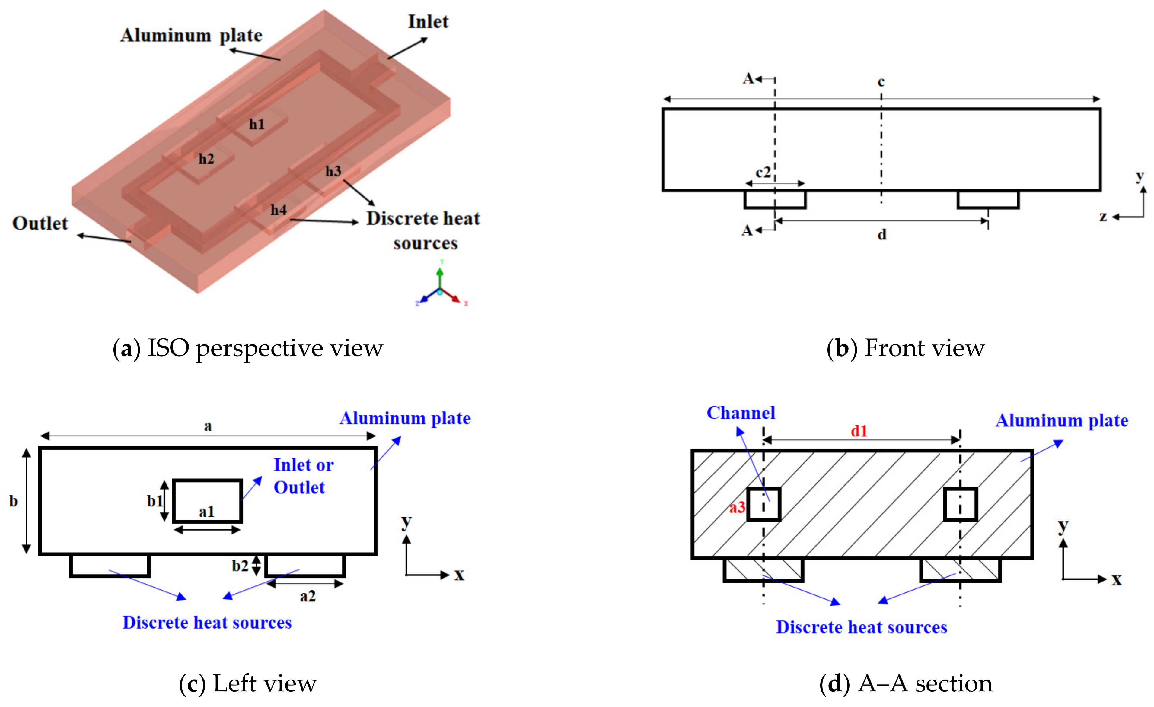
2.1. Physical Model

Based on literature research, it can be seen that the two-phase-flow heat transfer effect of the square channel is better, so this paper designed a square parallel channel to dissipate four discrete heat sources. As shown in Figure 1, the parallel channels formed in the aluminum plate are symmetrically distributed along the x, y, and z axes in space. The central axis of the branch channel is parallel to the central axis of the discrete heat source. In addition, the four discrete heat sources are symmetrically distributed along the x axis. The geometric parameters are shown in Table 1.
The heating power of each discrete heat source is 60 W, and the solid walls are cooled by natural convection of air expected the solid walls of extended section, which are adiabatic. The ambient temperature is 15 °C. The inlet boundary is the mass flow boundary, which has a total mass flow of 0.015 kg/s, and the subcooling degree is 1.5 °C. The outlet boundary is the pressure boundary and operating pressure is 8 bar. Refrigerant R134a was used in the simulation; the properties of R134a are presented in Table 2. The heat source can be treated as heating copper.

2.2. Mathematical Model

2.2.1. Governing Equations

Mass conservation equation [6,7,8,9,10,13,17]:
t ( α l ρ l ) + ( α l ρ l v ) = S l + S m l
t ( α v ρ v ) + ( α v ρ v v ) = S v + S m v
α l + α v = 1
where α, ρ, and v are phase fraction, density, and velocity; Sl and Sv are the volumetric mass source terms; Sml and Smv are the mass transfer between the liquid phase and the vapor phase, which can be obtained in the phase-change model. Subscript “l” and “v” mean liquid phase and vapor phase.
Momentum conservation equation [6,7,8,9,10,13,17]:
t ( ρ v ) + ( ρ v v ) = P + [ μ ( v + v T ) ] + ρ g + F
ρ = ρ l α l + ρ v α v
μ = μ l α l + μ v α v
where P, μ, and t are pressure, viscosity, and time; g and F represent gravitational acceleration and interface-induced volume force. The surface tension of the interface is calculated by the continuum surface force model (CSF) model proposed by Brackbill et al. [33] According to the divergence theorem, the force at the surface can be expressed as a volume force used in the momentum conservation equation. Thus, F is written as follows:
F = σ l v α l ρ l κ v α v + α v ρ v κ l α l 0.5 ( ρ l + ρ v )
where σlv is surface tension coefficient, and κ v and κ l is surface curvature, which is defined as follows:
κ v = κ l = α v α v
Energy conservation equation:
t ( ρ E ) + [ v ( ρ E + P ) ] = ( k T ) + S e
E = α l ρ l E l + α v ρ v E v α l ρ l + α v ρ v
k = k l α l + k v α v
where E, k, and T are energy per kilogram, coefficient of thermal conductivity, and temperature, and Se is the volumetric energy source term.

2.2.2. Phase Change Model

The phase change model is proposed to provide the mass transfer Sml and Smv and the energy source term Se between the liquid phase and the vapor phase due to the boiling. In this paper, the evaporation–condensation phase change model proposed by Lee [34] was used.
According to the theory of gas dynamics, the mass flux through the phase interface during the phase transition can be expressed as follows:
S m = β M 2 π R T s a t ( P v P s a t )
where β is the correction factor because the experimental theoretical evaporation is different. M is the molecular weight and R is the universal gas constant. Tsat means saturation temperature. In order to maintain equilibrium between the liquid and gas phases, the chemical potential energy should be equal, so the equation between pressure and temperature can be obtained using the Clausius–Clapeyron equation:
P v P s a t = h l v T ( 1 / ρ v 1 / ρ l ) ( T v T s a t )
where hlv is latent heat and Psat means saturation pressure. Assuming that the bubbles have the same diameter dp, the area density of the phase interface is given as:
1 A = 6 α v α l d p
Therefore, the mass transfer between the liquid phase and the vapor phase can be written as:
S m = A S m = 6 d p β M 2 π R T s a t h l v [ α v ρ v ( ρ l ρ v ) ] ( α l ρ l T T s a t T s a t )
To simplify the equations, the time relaxation factor parameters λl and λv are defined as:
λ l = 6 d p β M 2 π R T s a t h l v [ α v ρ v ( ρ l ρ v ) ] λ v = 6 d p β M 2 π R T s a t h l v [ α l ρ l ( ρ l ρ v ) ]
The mass transfer between the liquid phase and the vapor phase, Sml and Smv, can be written as follows:
S m v = λ l α l ρ l T T s a t T s a t ,   S m l = S m v T > T s a t S m l = λ v α v ρ v T s a t T T s a t ,   S m v = S m l T < T s a t
Thus, the energy source term can be calculated by the following equation:
S e = h l v S v
The time relaxation factors λl and λv should have appropriate values. If the value is too large, the calculation diverges easily and if the value is too small, the interface temperature deviates too much from the saturation temperature. Actually, the time relaxation factor is usually set as 0.1–100, referring to the studies by Lee [34] and Yang [17]. In this paper, λl and λv was set as 100 s−1 in order to maintain numerically the interface temperature within ±1 K compared with saturation temperature.

2.2.3. Solution Methods

Based on the pressure-based segregated solver with PISO scheme, the finite element method (FEM) was applied for solving the governing equations. The Green–Gauss node-based method was chosen to solve the gradient algorithm PRESTO!, which was selected for pressure dispersion. In order to ensure accuracy, the momentum and energy equations are discretized by the second-order upwind scheme. When the residual of all equations is less than 10−4, the simulation is considered as convergence and the implicit body force is opened to ensure the convergence of numerical simulation.

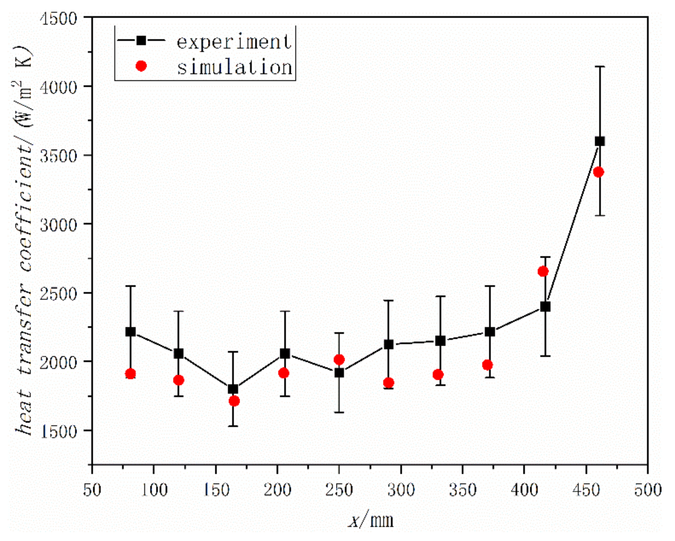
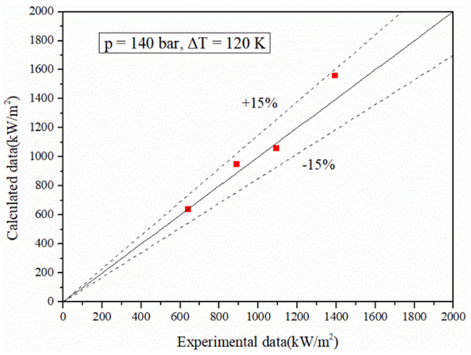
2.3. Validation of the Simulated Method

In order to validate the accuracy of the simulation model, the same numerical model (VOF and evaporation–condensation phase change model) and same solution method (PISO) used in the present study were adopted to simulate the experimental study by Lin et al. [35]. Lin investigated two-phase heat transfer to R141b in the minichannel heated at the heat flux of 30,000 W/m2. According to the work of Lin, the boundary conditions of inlet and outlet were velocity boundary (0.42 m/s) and pressure boundary, and the number of cells is 160,979. Based on simulation and experimental data, the variation of heat transfer coefficient along the channel is shown in Figure 2, and the definition of the heat transfer coefficient is written as follows:
h = q ( T ¯ w a l l T ¯ )
where q, T ¯ w a l l , and T ¯ are the heat flux, average temperature of the wall, and the average temperature of fluid in the cross-section.
From Figure 2, it can be seen that the deviation between experimental results and numerical value is less 15%, which shows that the simulated method is fully validating.
The grid sensitivity analysis on the result is indicated in Table 3. In order to ensure the solution accuracy and save on calculation time simultaneously, Mesh2 was selected.

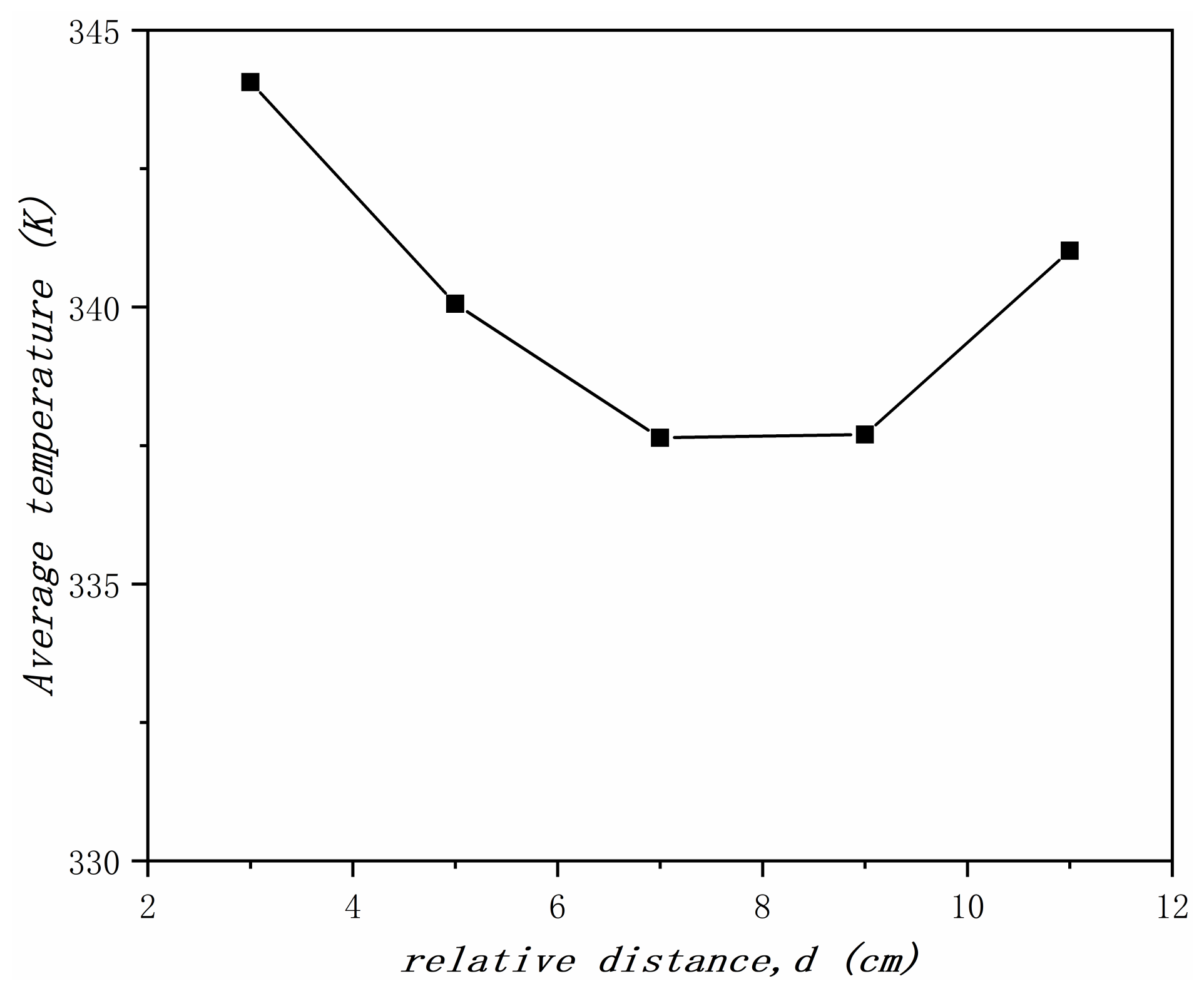
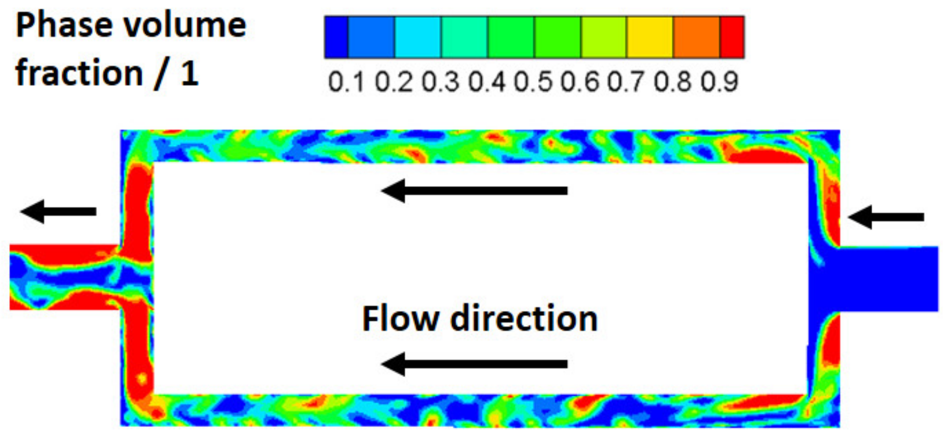
2.4. Results and Discussion

In order to explore the influence of the relative position of discrete heat sources on the heat transfer characteristics of two-phase flow, the relative distances on the z-axis for two discrete heat sources in the same branch channel were changed to 3, 5, 7, 9 and 11 cm (d = 3/5/7/9/11 cm, respectively) and controlled other factors unchanged. Meanwhile, the group in which the single continuous heat source heated the aluminum plate with the same total heating power was treated as the control group. The average temperature of the single continuous heat source is 331.76 K. It can be seen from Figure 3 that the average temperature of four discrete heat sources is higher than that of the continuous heat source. The reason why the heat transfer effect of the cold plate is better when heated by a continuous heat source is because the heat exchange area of the continuous heat source is larger than that of the discrete heat source, and the refrigerant is heated more evenly. In addition, Figure 3 also shows that the heat transfer effect of two-phase flow is different when the relative position of the discrete heat source is different. In this paper, when the z-axis relative distance of two discrete heat sources in the same branch channel is 7–9 cm, the heat transfer effect of the two-phase flow is the best, and the heat transfer effect is the worst when the discrete heat source distribution is closest.
When the z-axis relative distance of two discrete heat sources in the same branch channel is 7–9 cm, the two heat sources are close to the inlet and outlet of the channel, where the flow pulsation is more intense because the fluid direction changes and the fluid converges and disperses. Furthermore, it can be seen from Figure 4 that it is easier to nucleate and form bubbles at the corner of the flow channel. Therefore, the heat transfer capability of the inlet and outlet of the parallel channel is strong. In addition, the relative distance between discrete heat sources is large, so that the total heat will not be too concentrated, resulting in heat transfer deterioration. Thus, when the z-axis relative distance of two discrete heat sources is 7–9 cm, the temperature of the heat source is the lowest. On the contrary, when the distribution of discrete heat sources is closer, the more concentrated the total heat. If the heat is too concentrated, then it is easy to produce numerous bubbles and to form a gas film, which is not conducive to heat dissipation.
When cooling the multiple chips, the temperature uniformity is also an important evaluation index. Uneven temperature distribution will generate thermal stress and affect the service life of the equipment. In Figure 5, “Heat source h1, h2, h3, h4” along the x-axis means four discrete heat sources; the location of the four discrete heat sources can be seen in Figure 1. The ordinate of Figure 5 represents the average temperature of heat sources. As shown in Figure 5, the two-phase flow heat transfer is helpful to improve the temperature nonuniformity and when the z-axis relative distance of two discrete heat sources in the same branch channel is 9 cm, the temperature distribution of the heat sources is most uniform.

3. Analysis of Flow Instability

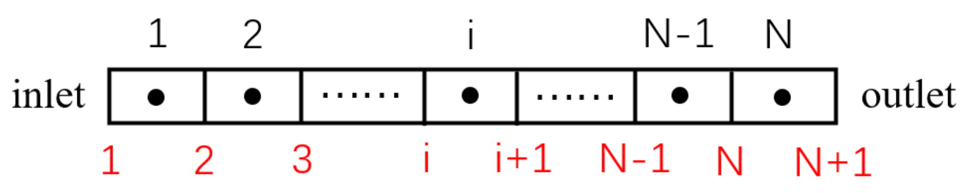
3.1. Mathematical Model

Numerical methods for studying flow instability can be divided into two types: frequency domain method and time domain method. It should be noted that the frequency domain method can significantly shorten the time for numerical calculation through Laplace transform and linearization of the equation, but it cannot solve complex nonlinear problems. In this paper, the time domain method, referring to the investigations of Lu et al. [18] and Ma et al. [36], is adopted to analyze the flow instability.
Compared with heat transfer between fluid and channels, the investigation on flow instability pays greater attention to the axial changes of parameters instead of the one on cross-section. In order to effectively simplify the calculation, the following reasonable assumptions are made for the model:
  • It is simplified to one-dimension, and only the variation of the parameters in the axial direction is considered;
  • The entire tube is in thermal equilibrium;
  • The fluid at the inlet of the pipeline is always in a state of supercooling;
  • Subcooled boiling is not taken into account in the subcooling zone of the pipeline. The simplified physical model is shown in Figure 6.
The homogeneous flow model is adopted, and the corresponding governing equations follow.
Mass conservation equation:
ρ t + ρ u z = 0
Momentum conservation equation:
ρ u t + ρ u 2 z = p z ρ g λ D e + k ρ u 2 2
where k is defined as:
Δ p L = k ρ u 2 2
Energy conservation equation:
ρ h t + ρ u h z = q + p t
Equation of state:
ρ = ρ   p , h
When the fluid is in two-phase state:
h = x h g + ( 1 x ) h l
ρ = α ρ g + ( 1 α ) ρ l
u g u l = 1 = 1 α α x 1 x ρ l ρ g
where ρ, u, h, p, x, and α are density, velocity, enthalpy, pressure, mass quality, and void fraction of fluid, respectively. The subscript g represents vapor, and the subscript l represents liquid. In addition, t means time and z refers to the axial coordinate, and q, g, λ, De, k, and ΔpL are thermal power per unit volume, gravitational acceleration, Darcy friction coefficient, hydraulic diameter, the throttling coefficient at the inlet or outlet, and local resistance pressure drop, respectively.
A staggered grid is used in this paper, in which p, ρ, and h are stored at the center of the control volume, while u is stored at the boundary of the control volume, as shown in Figure 7.
The first order upwind difference and semi-implicit scheme are employed to discretize the equation, and the following equations can be obtained by the chain rule of partial derivatives.
Mass conservation equation:
ρ h i h i n h i Δ t + ρ p i p i n p i Δ t + ρ i u i + 1 n ρ i 1 u i n Δ z = 0
Momentum conservation equation:
ρ i u i + 1 n ρ i u i + 1 Δ t + ρ i + 1 u i + 1 2 ρ i u i 2 Δ z + p i + 1 n p i n Δ z + λ i D e + k i ρ i u i + 1 2 2 + ρ i g = 0
ρ i 1 u i n ρ i 1 u i Δ t + ρ i u i 2 ρ i 1 u i 1 2 Δ z + p i n p i 1 n Δ z + λ i 1 D e + k i 1 ρ i 1 u i 2 2 + ρ i 1 g = 0
Energy conservation equation:
h i ρ h i + ρ i h i n h i Δ t + h i ρ p i 1 p i n p i Δ t + ρ i h i u i + 1 n ρ i 1 h i 1 u i n Δ z = q
where the superscript n and the subscript i represent the next time level and the control volume sequence number, respectively, while Δt and Δz represent the time step and the space step.
Assuming that all parameters of the current time level are known, combining and simplifying Equations (24)–(27) gives the following form:
A 1 , i δ p i 1 + A 2 , i δ p i + A 3 , i δ p i + 1 = B i
where δp = pnp is the pressure difference between the next and the current time level. In addition, Aj (j = 1,2,3) and B are constants.
In order to eliminate the step of flow distribution and improve the calculation speed in the program, the upper header and the subheader are divided into two control volumes, and then the discretization is carried out in the same way as noted above. The matrix equation of the whole system can be obtained by integrating Equation (33) for every control volume:
A 1 , 1 A 1 , 2 A 1 , 2 N + 1 A 1 , 2 N + 2 A 2 , 1 A 2 , 2 A 2 , 2 N + 1 A 2 , 2 N + 2   A 2 N + 1 , 1 A 2 N + 1 , 2 A 2 N + 1 , 2 N + 1 A 2 N + 1 , 2 N + 2 A 2 N + 2 , 1 A 2 N + 2 , 2 A 2 N + 2 , 2 N + 1 A 2 N + 2 , 2 N + 2 δ p 1 δ p 2 δ p 2 N + 1 δ p 2 N + 2 = B 1 B 2 B 2 N + 1 B 2 N + 2
δp in Equation (32) can be calculated by the Gaussian elimination method, and then the remaining unknowns, including un, hn, ρn, can be determined by substituting δp back into Equations (24) and (28)–(30), respectively. The numerical computations noted are implemented by FORTRAN codes.

3.2. Solution Method and Model Validation

The transient calculation is performed while an initial field of system is given. After running for a sufficiently long time, the system reaches steady state when the flow rate of each tube does not change over time and the thermal disturbance is now applied, that is, the thermal power of a tube increases by 0.1%. After a short time, e.g., 0.01 s, the thermal power is restored to its original state, which is equal to a pulse consisting of two step functions, and then the changes of flow rate in the two tubes are observed.
If divergent oscillation occurs, that is, the amplitude of the oscillation of two tubes becomes increasingly larger, that means the thermal power is too high. Otherwise, it is a damped oscillation. Until the oscillation becomes a constant amplitude, the thermal power at this time is the critical thermal power. As shown in Figure 8, when the degree of inlet subcooling is 30 K and the total thermal power is 4730.6 W, the parallel channel oscillates in constant amplitude as a result of the thermal disturbance noted above according to the parameters set in Table 4.
By comparing the set model with experimental data [37], it can be found that when the pressure of the system is 140 bar and the inlet undercooling degree is 120 K, different total critical thermal power per unit area of system can be obtained for different total mass flow, as shown in Figure 9. The errors between the calculated values and the experimental values are within ±15%, which indicates that the two are in excellent agreement, and the correctness of the model is verified.

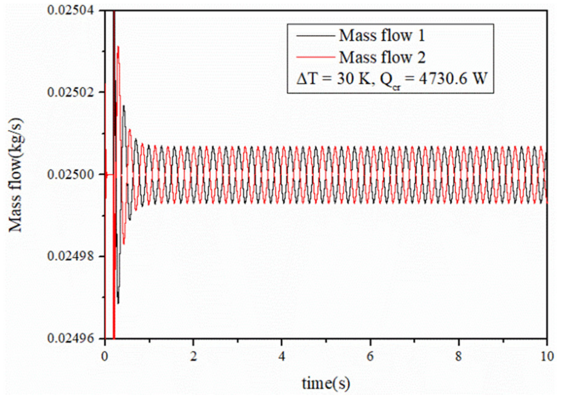
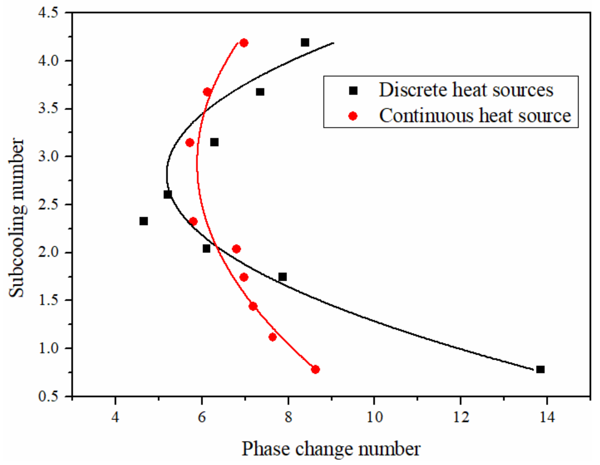
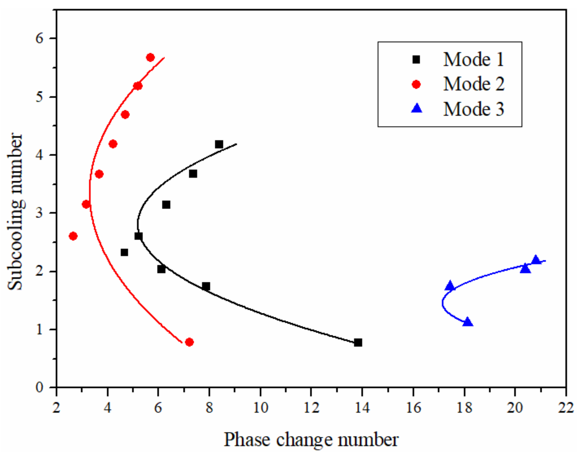
3.3. Result and Discussion

In the study of flow instability, the two-dimensional plane composed of dimensionless numbers, Npch and Nsub, is generally used to characterize the stability boundary. Npch means the phase change number and Nsub represents the subcooling number. Their definitions follow:
N p c h = Q W ρ f ρ g h f g ρ g
N s u b = Δ h i n ρ f ρ g h f g ρ g
where Q, W, and hfg refer to heating power, mass flow rate, and latent heat of vaporization. Additionally, Δhin = hlhin is undercooling enthalpy of the inlet. The physical properties and geometric parameters as shown in Table 3 are used for calculation, and the flowing medium is water.
First, the influence of discrete and continuous heat source distribution on flow instability under the same total heating power is analyzed. The continuous distribution of the heat source is shown in Figure 6 while the setting of the discrete heat source for comparison is shown in Figure 10. In order to be representative, the discrete heat sources are set to be uniformly distributed along the pipe segment, and each pipe has two discrete heat sources. Calculated according to the parameters in Table 3, the stability boundary finally obtained is shown in Figure 11. When the inlet undercooling degree is relatively low and relatively high, the stability boundary of the discrete heat source is located on the right of the continuous heat source boundary, which indicates that the flow of discrete heating is more stable than that of continuous heating. However, when the inlet undercooling is moderate, the stability of the continuous heat source is better than that of the discrete heat source. The analysis shows that when the inlet undercooling degree is low, the fluid is heated by the discrete heat source with high heat flux and directly turns into single-phase steam. When the degree of undercooling at the inlet is high, the enthalpy of the fluid is still at a low value even after passing through the discrete heat source, and the nonheated section of the channel is basically in the undercooled region. Regardless of whether the fluid in most channels is in gas or liquid phase, its density does not change dramatically, thus inhibiting the occurrence of flow instability. However, when the degree of undercooling at the inlet is within a specific range, resulting in the fluid heated by the discrete heat source just being in the two-phase region, the nonheated region is equivalent to extending the two-phase region, that is, the region with periodic changes of density is prolonged, causing the deterioration of the flow stability.
The numerical distribution of discrete heat sources also affects the flow instability. For the discrete heat source shown in Figure 10, keeping the position of the heat source and the total heating power of the single tube unchanged, but changing the respective proportion of total heating. power The working conditions are set as shown in Table 5. Heat source 1 and heat source 2 refer to the discrete heat source near the inlet and outlet, respectively. A stability boundary diagram of three working conditions is shown in Figure 12. The results show that the numerical distribution of the discrete heat source, which can affect the flow stability, is not only related to the uniformity but also relevant to the distribution sequence along the flow path. In the stability boundary diagram, the order from left to right is working conditions 2, 1, and 3, which is also the order in which the stability gradually improves. It can be considered that the greater the power of the discrete heat source close to the inlet and the smaller the power close to the outlet, the worse the flow stability will be, and vice versa. This can be attributed to the fact that the high-power discrete heat source close to the inlet rapidly increases the enthalpy of the fluid, resulting in drastic changes in the density of the fluid in most of the subsequent flow channels, thus promoting the occurrence of flow instability. However, when the high-power heat source is near the outlet, the enthalpy value of most fluids in the flow passage is low and the density changes little. Even if the density changes dramatically after heating by the heat source, the remaining flow passage is not enough to fully show the flow instability. Thus, flow stability is improved when the high-power discrete heat source is closer to the flow outlet or the low-power discrete heat source is closer to the flow inlet.

4. Conclusions

In this paper, the two-phase heat transfer characteristics and instability in parallel channels with discrete heat source arrangement were studied by numerical simulation. The main conclusions are as follows:
(1)
The relative positions of discrete heat sources affect the heat transfer effect of two-phase flow, and the heat transfer performance can be improved by reasonably designing the relative position of heat sources.
(2)
The closer the distribution of discrete heat sources, the worse the heat transfer effect; for the working condition designed in this paper, the heat transfer effect is best when the distance between the centers of the two discrete heat sources on the same branch channel are within a range of 7–9 cm.
(3)
Compared with the continuous heat source, the discrete heat source with uniform distribution can enhance the flow stability under low and high inlet undercooling.
(4)
When the high-power discrete heat source is closer to the flow outlet and the low-power discrete heat source is closer to the flow inlet, the flow stability is improved.

Author Contributions

Conceptualization, C.H., R.W. and M.Z.; methodology, C.H., R.W., P.Y. and W.L.; software, P.Y. and W.L.; validation, P.Y. and W.L.; formal analysis, P.Y. and W.L.; investigation, C.H., R.W. and J.Q.; resources, C.H., R.W., J.Q., Q.W. and M.Z.; data curation, P.Y. and W.L.; writing—original draft preparation, C.H., P.Y. and W.L.; writing—review and editing, M.Z., J.Q. and Q.W.; project administration, C.H., R.W., M.Z., Q.W. and J.Q. All authors have read and agreed to the published version of the manuscript.

Funding

This research received no external funding.

Institutional Review Board Statement

The study did not involve humans or animals.

Informed Consent Statement

The study did not involve humans.

Data Availability Statement

The study did not report any data.

Conflicts of Interest

The authors declare no conflict of interest.

References

  1. Rosa, P.; Karayiannis, T.G.; Collins, M.W. Single-phase heat transfer in microchannels: The importance of scaling effects. Appl. Therm. Eng. 2011, 29, 3447–3468. [Google Scholar] [CrossRef] [Green Version]
  2. Agostini, B.; Fabbri, M.; Park, J.E.; Wojtan, L.; Thome, J.R.; Michel, B. State-of-the-art of high heat flux cooling technologies. Heat Transf. Eng. 2007, 28, 258–281. [Google Scholar] [CrossRef]
  3. Yen, T.H.; Shoji, M.; Takemura, F.; Suzuki, Y.; Kasagi, N. Visualization of convective boiling heat transfer in single microchannels with different shaped cross-sections. Int. J. Heat Mass Transf. 2006, 49, 3884–3894. [Google Scholar] [CrossRef]
  4. Deng, D.; Wan, W.; Tang, Y.; Wan, Z.; Liang, D. Experimental investigations on flow boiling performance of reentrant and rectangular microchannels-a comparative study. Int. J. Heat Mass Transf. 2015, 82, 435–446. [Google Scholar] [CrossRef]
  5. Tran, N.T.; Chyub, M.C. Two-phase pressure drop of refrigerants during flow boiling in small channels: An experimental investigation and correlation development. Int. J. Multiph. Flow 2000, 26, 1739–1754. [Google Scholar] [CrossRef] [Green Version]
  6. Meng, M.; Yang, Z.; Duan, Y.Y.; Chen, Y. Boiling flow of R141b in vertical and inclined Serpentine Tubes. Int. J. Heat Mass Transf. 2013, 57, 312–320. [Google Scholar] [CrossRef]
  7. Huang, F.; Zhao, J.; Zhang, Y.; Zhang, H.; Wang, C.; Liu, Z. Numerical analysis on flow pattern and heat transfer characteristics of flow boiling in the mini-channels. Numer. Heat Transf. Part. B Fundam. 2020, 78, 221–247. [Google Scholar] [CrossRef]
  8. Gorlé, C.; Lee, H.; Houshmand, F.; Asheghi, M.; Goodson, K.; Parida, P.R. Validation study for VOF simulations of boiling in a microchannel. In International Electronic Packaging Technical Conference and Exhibition, Proceedings of the ASME 2015 13th International Conference on Nanochannels, Microchannels, and Minichannels (InterPACK2015), San Francisco, CA, USA, 6–9 July 2015; American Society of Mechanical Engineers: New York, NY, USA, 2015; Volume 56901, p. V003T10A022. [Google Scholar]
  9. Lorenzini, D.; Joshi, Y. CFD study of flow boiling in silicon microgaps with staggered pin fins for the 3D-stacking of ICs. In Proceedings of the 2016 15th IEEE Intersociety Conference on Thermal and Thermomechanical Phenomena in Electronic Systems (ITherm), Las Vegas, NV, USA, 31 May–3 June 2016. [Google Scholar]
  10. Lee, H.; Agonafer, D.D.; Won, Y.; Houshmand, F.; Gorle, C.; Asheghi, M.; Goodson, K.E. Thermal Modeling of Extreme Heat Flux Microchannel Coolers for GaN-on-SiC Semiconductor Devices. J. Electron. Packag. 2016, 138, 10907. [Google Scholar] [CrossRef] [Green Version]
  11. Vontas, K.; Andredaki, M.; Georgoulas, A.; Miché, N.; Marengo, M. The effect of surface wettability on flow boiling characteristics within microchannels. Int. J. Heat Mass Transf. 2021, 172, 121133. [Google Scholar] [CrossRef]
  12. Li, X.; Wei, W.; Wang, R.; Shi, Y. Numerical and experimental investigation of heat transfer on heating surface during subcooled boiling flow of liquid nitrogen. Int. J. Heat Mass Transf. 2009, 52, 1510–1516. [Google Scholar] [CrossRef]
  13. Soleimani, A.; Sattari, A.; Hanafizadeh, P. Thermal analysis of a microchannel heat sink cooled by two-phase flow boiling of Al2O3 HFE-7100 nanofluid. Therm. Sci. Eng. Prog. 2020, 20, 100693. [Google Scholar] [CrossRef]
  14. Zhuan, R.; Wang, W. Simulation on nucleate boiling in micro-channel. Int. J. Heat Mass Transf. 2010, 53, 502–512. [Google Scholar] [CrossRef]
  15. Liu, Q.; Palm, B. Numerical study of bubbles rising and merging during convective boiling in micro-channels. Appl. Therm. Eng. 2016, 99, 1141–1151. [Google Scholar] [CrossRef]
  16. Yu, J.; Ma, H.; Jiang, Y. A numerical study of heat transfer and pressure drop of hydrocarbon mixture refrigerant during boiling in vertical rectangular minichannel. Appl. Therm. Eng. 2017, 112, 1343–1352. [Google Scholar] [CrossRef]
  17. Yang, Z.; Peng, X.F.; Ye, P. Numerical and experimental investigation of two phase flow during boiling in a coiled tube. Int. J. Heat Mass Transf. 2008, 51, 1003–1016. [Google Scholar] [CrossRef]
  18. Hardt, S.; Herbert, S.; Kunkelmann, C.; Mahjoob, S.; Stephan, P. Unidirectional bubble growth in microchannels with asymmetric surface features. Int. J. Heat Mass Transf. 2012, 55, 7056–7062. [Google Scholar] [CrossRef]
  19. Ma, H.; Cai, W.; Chen, J.; Yao, Y.; Jiang, Y. Numerical investigation on saturated boiling and heat transfer correlations in a vertical rectangular minichannel. Int. J. Therm. Sci. 2016, 102, 285–299. [Google Scholar] [CrossRef]
  20. Cho, E.S.; Choi, J.W.; Yoon, J.S.; Kim, M.S. Modeling and simulation on the mass flow distribution in microchannel heat sinks with non-uniform heat flux conditions. Int. J. Heat Mass Transf. 2010, 53, 1341–1348. [Google Scholar] [CrossRef]
  21. Cho, E.S.; Choi, J.W.; Yoon, J.S.; Kim, M.S. Experimental study on microchannel heat sinks considering mass flow distribution with non-uniform heat flux conditions. Int. J. Heat Mass Transf. 2010, 53, 2159–2168. [Google Scholar] [CrossRef]
  22. Bhowmik, H.; Tso, C.P.; Tou, K.W.; Tan, F.L. Convection heat transfer from discrete heat sources in a liquid cooled rectangular channel. Appl. Therm. Eng. 2005, 25, 2532–2542. [Google Scholar] [CrossRef]
  23. Kurose, K.; Miyata, K.; Hamamoto, Y.; Mori, H. Flow boiling heat transfer and flow distribution of HFC32 and HFC134a in unequally heated parallel mini-channels. Int. J. Refrig. 2020, 119, 305–315. [Google Scholar] [CrossRef]
  24. Islam, M.A.; Pal, A.; Thu, K.; Saha, B.B. Study on performance and environmental impact of supermarket refrigeration system in Japan Evergreen. Evergreen 2019, 6, 168–176. [Google Scholar] [CrossRef]
  25. Kurose, K.; Noboritate, W.; Sakai, S.; Miyata, K.; Hamamoto, Y. An experimental study on flow boiling heat transfer of R410A in parallel two mini-channels heated unequally by high-temperature fluid. Appl. Therm. Eng. 2020, 178, 1359–4311. [Google Scholar] [CrossRef]
  26. Ghaedamini, H.; Salimpour, M.R.; Mujumdar, A.S. The effect of svelteness on the bifurcation angles role in pressure drop and flow uniformity of tree-shaped microchannels. Appl. Therm. Eng. 2011, 31, 708–716. [Google Scholar] [CrossRef]
  27. Colombo, M.; Cammi, A.; Papini, D.; Ricotti, M.E. RELAP5/MOD3.3 study on density wave instabilities in single channel and two parallel channels. Prog. Nucl. Energy 2012, 56, 15–23. [Google Scholar]
  28. Paruya, S.; Maiti, S.; Karmakar, A.; Gupta, P.; Sarkar, J.P. Lumped parameterization of boiling channel—Bifurcations during density wave oscillations. Chem. Eng. Sci. 2012, 74, 310–326. [Google Scholar] [CrossRef]
  29. Papini, D.; Cammi, A.; Colombo, M.; Ricotti, M.E. Time-domain linear and non-linear studies on density wave oscillations. Chem. Eng. Sci. 2012, 81, 118–139. [Google Scholar] [CrossRef]
  30. Lu, X.; Wu, Y.; Zhou, L.; Tian, W.; Su, G.; Qiu, S.; Zhang, H. Theoretical investigations on two-phase flow instability in parallel channels under axial non-uniform heating. Ann. Nucl. Energy 2014, 63, 75–82. [Google Scholar] [CrossRef]
  31. Paul, S.; Singh, S. Linear stability analysis of flow instabilities with a nodalized reduced order model in heated channel. Int. J. Therm. Sci. 2015, 98, 312–331. [Google Scholar] [CrossRef]
  32. Paul, D.; Singh, S.; Mishra, S. Impact of system pressure on the characteristics of stability boundary for a single-channel flow boiling system. Nonlinear Dyn. 2019, 96, 175–184. [Google Scholar] [CrossRef]
  33. Brackbill, J.U.; Kother, D.B.; Zemach, C. A continuum method for modeling surface tension. J. Comput. Phys. 1992, 100, 335–354. [Google Scholar] [CrossRef]
  34. Lee, W.H. A Pressure Iteration Scheme for Two-phase Flow Modeling. In Multiphase Transport. Fundamentals, Reactor Safety, Applications; Veziroglu, T.N., Ed.; Hemisphere Publishing: Washington, DC, USA, 1980; pp. 407–432. [Google Scholar]
  35. Lin, S.; Kew, P.A.; Cornwell, K. Two-phase heat transfer to a refrigerant in a 1 mm diameter tube. Int. J. Refrig. 2001, 24, 51–56. [Google Scholar] [CrossRef]
  36. Ma, Z.; Zhang, L.; Bu, S.; Sun, W.; Chen, D.; Pan, L. A study of the heat flux profile effect on parallel channel density wave oscillation in sodium heated heat exchanger. Prog. Nucl. Energy 2019, 112, 135–145. [Google Scholar] [CrossRef]
  37. Zhou, Y.L.; Shen, Z.M.; Jing, J.G.; Chen, T.K. Experimental study on density wave instability of high pressure vapor-liquid two-phase flow in parallel pipes. J. Eng. Thermophys. 1996, 17, 215–218. [Google Scholar]
Figure 1. Schematic of geometry.
Energies 14 04408 g001
Figure 2. Comparison between experiment and simulation.
Energies 14 04408 g002
Figure 3. Comparison of average temperature of heat source.
Energies 14 04408 g003
Figure 4. Two-phase flow regimes of parallel channels (y = 0.005 m).
Energies 14 04408 g004
Figure 5. Temperature of different discrete heat sources.
Energies 14 04408 g005
Figure 6. Schematic of the parallel channels model.
Energies 14 04408 g006
Figure 7. Staggered grid.
Energies 14 04408 g007
Figure 8. Constant amplitude oscillation at critical thermal power.
Energies 14 04408 g008
Figure 9. Comparison of calculated and experimental data.
Energies 14 04408 g009
Figure 10. Uniform distribution of discrete heat sources.
Energies 14 04408 g010
Figure 11. Stability boundary of discrete and continuous heat sources.
Energies 14 04408 g011
Figure 12. Stability boundary of discrete heat source with different numerical distribution.
Energies 14 04408 g012
Table 1. Geometric parameters.
ParameterValue
Volume of aluminum plate (c × a × b)/cm314 × 7 × 1
Volume of discrete heat sources (c2 × a2 × b2)/cm32 × 2 × 0.3
Volume of single continuous heat source/cm314 × 7 × 0.3
Cross section area of inlet (a1 × b1)/cm21 × 0.5
Cross section area of outlet (a1 × b1)/cm21 × 0.5
Cross section area of branch (a3 × a3)/cm20.5 × 0.5
Axis distance of parallel channel (d1)/cm4
Table 2. Properties of R134a.
PropertiesLiquidVapor
Density ρ/(kg/m3)1182.239.025
Viscosity μ/(kg/(m s))0.000180110.000011965
Coefficient of thermal conductivity k/(W/(m K))0.0784240.014497
Specific heat capacity CP/(J/(kg K))1452.739.025
Latent heat h/(kJ/kg)171.81
Surface tension σ /(N/m)0.0072429
Saturation temperature Tsat/K304.48
Table 3. Grid independence verification.
CaseGrid Number 1Average Temperature of 4 Discrete Heat Sources Th/K ( T h j T h j ) / T h j
Mesh1361061337.02.37 × 10−3
Mesh2392049337.82.07 × 10−3
Mesh3432322338.55.91 × 10−4
Mesh4545087338.7-
Table 4. Parameters of fluid and geometry.
ParameterValue
Heated length/(mm)140
Cross section of channel/(mm2)5 × 10
System pressure/(MPa)14
Total mass flow/(kg/s)0.015
Inlet subcooling/(K)10–40
Channel inclination/(°)90
Table 5. Different numerical distributions of discrete heat sources.
Discrete Heat SourceProportion of Total Heating Power
Mode 1Mode 2Mode 3
Source 10.50.10.1
Source 20.50.10.9
Publisher’s Note: MDPI stays neutral with regard to jurisdictional claims in published maps and institutional affiliations.

