
Modelling Yawed Wind Turbine Wakes: Extension of a Gaussian-Based Wake Model


1
Computational Marine Hydrodynamics Lab (CMHL), School of Naval Architecture, Ocean and Civil Engineering, Shanghai Jiao Tong University, Shanghai 200240, China
2
Key Laboratory of Far-Shore Wind Power Technology of Zhejiang Province, Power China Huadong Engineering Corporation Limited, Hangzhou 310014, China
3
Ocean College, Zhejiang University, Zhoushan 316021, China
*
Author to whom correspondence should be addressed.
Energies 2021, 14(15), 4494; https://0-doi-org.brum.beds.ac.uk/10.3390/en14154494
Submission received: 26 May 2021
/
Revised: 18 July 2021
/
Accepted: 22 July 2021
/
Published: 25 July 2021
(This article belongs to the Special Issue Recent Advances in Offshore Wind Turbines)
Abstract
:Yaw-based wake steering control is a potential way to improve wind plant overall performance. For its engineering application, it is crucial to accurately predict the turbine wakes under various yawed conditions within a short time. In this work, a two-dimensional analytical model is proposed for far wake modeling under yawed conditions by taking the self-similarity assumption for the streamwise velocity deficit and skewness angle at hub height. The proposed model can be applied to predict the wake center trajectory, streamwise velocity, and transverse velocity in the far-wake region downstream of a yawed turbine. For validation purposes, predictions by the newly proposed model are compared to wind tunnel measurements and large-eddy simulation data. The results show that the proposed model has significantly high accuracy and outperforms other common wake models. More importantly, the equations of the new proposed model are simple, the wake growth rate is the only parameter to be specified, which makes the model easy to be used in practice.
1. Introduction
With the rapid growth in demand for renewable resources, wind energy production has aroused more and more attention. To maximize the wind resources in limited available lands and reduce the maintenance costs, wind turbines are commonly installed together in wind power plants. An accompanying drawback is the complex wake effects, including a lower wind speed and an enhanced turbulence intensity level. Research [1] has revealed that, compared with the ideal un-wake state, the power loss of the wind farm caused by wakes can up to 20%. Apart from decreased energy capture, the high turbulence intensity level in the wake region also increases fatigue and dynamic loads for the downstream turbines, and further, affecting their lifetimes [2,3].
In order to mitigate wake interferences, different active wake control strategies were proposed and investigated in recent years. For example, reducing the axial induction of the upstream wind turbine by adjusting tip speed ratio, blade pitch, or torque has been studied in [4,5,6]. Another promising approach is to redirect turbine wake by an intentional yaw misalignment [7,8], which is implemented by altering the yaw angle of the upwind turbine intentionally when it is aligned to the inflow wind direction. By doing so, the wake trajectory of the controlled upstream turbine will deviate from the inline downstream wind turbines, whereby the latter can capture more energy from the wake flow and compensate for the power loss of the upstream turbine in a global view. For an application of such an operation control, it is crucial to fully understand the wake characteristics of the yawed wind turbine under various conditions.
The first effort to study the yawed turbine wake was made by Jimenez et al. [9], who used large eddy simulation, together with the actuator disk model, to investigate the wake deflection and trajectory under a range of yaw angles and thrust coefficients. For the given model parameters in their study, a qualitative agreement was found in the comparison of the LES results, analytical model, and experimental data. By applying open source CFD tool SOWFA, Fleming et al. [10,11] tested several possible approaches on redirecting turbine wakes, and the results showed that yaw angle control is a more effective method for wake deviation, compared to other proposed control strategies, such as modifying the tilt angle or downrating through blade pitch control. Furthermore, in the studies of Wang et al. [12] and Miao et al. [13], similar conclusions were also obtained. Gebraad et al. [14] later conducted a numerical investigation on wind farm power optimization by altering the yaw settings of wind turbines. They found that wind plant control based on yaw misalignment can increase electrical power generation for different configurations of the wind farm and reduce the loading on downstream wind turbines. In the work of Vollmer et al. [15], the difference in wake shape and wake deflection downstream of a yawed turbine was explored under three typical atmospheric thermal stabilities, and an increase in the uncertainty of wake deflection estimation was found with decreasing atmospheric stability.
Apart from high fidelity numerical simulations, wind tunnel tests are also widely used in studying yawed turbine properties and wake features, as well as the effects of yaw angle control on the efficiency of wind farms.
Howland et al. [16] experimentally studied the wake deflection and wake shape in yawed conditions behind a porous disk model turbine, the measured velocity distribution and wake center trajectory at different downwind distances were compared with prior studies and model predictions. By using Laser Doppler anemometry, Schottler et al. [17] performed several wind tunnel tests to investigate wake features for different yaw angles, and a new method was introduced to parameterize the yawed wake shape. In order to better understand the interaction between the yawed turbine wake and the turbulent boundary layer, Bastankhah and Porté-Agel [18] carried out an experimental study on the performance of a model wind turbine and its wake in a neutral atmospheric condition under different yaw angles and tip speed ratios. The results suggested that as the yaw angle increases, both the power and thrust coefficients decrease, and the wake deflection increases. Additionally, a nonsymmetric flow distribution of the induced velocity was found upstream of the yawed wind turbine, it should be taken into account for the prediction of the loading distribution. Focusing on two tandem arranged wind turbines, Ozbay et al. [19] conducted wind tunnel measurements to assess the impact of the yaw behavior of upstream wind turbines on the overall performance of wind plants. They found that when the first wind turbine was operated at different yaw angles, the total power generation varied greatly, closely related to the turbulence intensity level of the incoming wind.
In real-world engineering scenarios, for example, when optimizing wind farms’ power by controlling yaw angles of wind turbines, in order to obtain the best yaw setting, it is necessary to examine each possible scheme. Obviously, under such conditions, relying on time-consuming numerical simulations or wind tunnel measurements is unfeasible. Furthermore, due to the impacts of atmospheric turbulence, thermal stability, etc. [20,21], the wind turbine is often exposed to a variable inflow environment. Therefore, assessing the effectiveness of yaw angle control under a wide variety of conditions is indispensable. To satisfy the fast prediction requirements in real engineering applications, developing simple and high-efficiency analytical models for the yawed turbine wake is needed, and many efforts have been made previously by researchers in the wind energy community.
According to the conservation of mass and momentum for a control volume around the yawed wind turbine, and the top-hat distribution assumption for both velocity deficit and skew angle profiles, Jimenez et al. [9] firstly proposed an analytical model to predict the yawed wake in which the skew angle is expressed as a function of yaw angle and thrust coefficient. Later, by integrating the skew angle, Gebraad et al. [14] and Howland et al. [22] obtained the wake center trajectory. However, as pointed out in references [23,24], the accuracy of such analytical models is questioned as the top-hat shape for velocity deficit profile is not realistic.
Based on measurements from high-resolution wind tunnel tests [18], Bastankhah and Porté-Agel [25] simplify the Reynolds-averaged Navier Stokes equations, combining with the self-similar Gaussian distributions for velocity deficit and skew angle profiles, they built a realistic analytical model for the far-wake region in yawed conditions. Although good consistency is found between the experimental results and model predictions, multiple parameters in the wake model need to be specified. In particular, to find the wake characteristics in the onset of the far-wake region, it is necessary to determine the length of the potential core, and for this purpose, values of two empirical parameters are supposed to be first estimated. However, as the author said, it is difficult to find the universal values, their estimations strongly depend on numerical simulations or wind tunnel experiments. Obviously, the applicability of the wake model is greatly limited. Different from the Bastankhah–Porté-Agel model that completely relied on the Gaussian assumption, Qian and Ishihara [26,27] later proposed another wake model, adopting a Gaussian distribution for velocity deficit, but a top-hat shape for skew angle. In that wake model, the input parameters are modeled as functions of ambient turbulence intensity and thrust coefficient, which is considered to enhance the model applicability, but more validation works are required.
In addition to the streamwise velocity, the transverse velocity, caused by the lateral force exerted by the yawed wind turbine on the incoming airflow, is also important. It deflects the wake of the yawed turbine itself to one side and deviates the wake trajectory of an aligned non-yawed downwind turbine from its centerline. Such a “secondary steering effect” has been reported in many previous studies [28,29] and is considered to have a great impact on the power generation for the wind farm under yawed conditions. Therefore, in the analytical wake models for yawed wind turbines, it is necessary to include the prediction for the transverse velocity. However, in the existing models [25,30], although researchers have conducted valuable analysis on the characteristics of transverse velocity, in real-world applications, these models cannot fully exploit their advantages since many model parameters are required and some are difficult to specify directly.
Different from the conventional analytical models based on the geometrical deflection at turbine hub height, researchers have also developed some three-dimensional (3D) models [29,31] including wake curling physics. However, studies in that field are not mature enough, and some important factors are not taken into account for the available versions of those models, for example, the added turbulence intensity induced by wind turbines and the vortex decay effect. This results in some differences between model predictions and the real yawed wake flow. As a consequence, models of this kind are rarely used in engineering projects at present.
As illustrated above, the potential of the wake steering strategy based on yaw angle control has been validated in a number of numerical simulations and wind tunnel measurements. Furthermore, considering the requirement for fast wake predictions in real engineering projects, such as deploying the real-time yaw control in wind farms or assessing the impact of control strategy on annual energy production, the importance of wake models is self-evident. However, there are still problems of effectiveness and universality for the existing commonly used analytical models. Therefore, it is essential to develop a simple model that can predict the key wake characteristics for the yawed turbine with acceptable accuracy.
The remainder of this paper is organized as follows: In Section 2, a brief introduction of the LES framework and numerical setup are presented. The simulation results for different yaw angles are displayed and analyzed in Section 3. Based on the simulation results and theoretical analysis, in Section 4, a new analytical model for predicting the wake deflection and streamwise velocity downstream of a yawed wind turbine is proposed and validated. In Section 5, the proposed new model is extended to incorporate the transverse velocity prediction in the far-wake region. Finally, conclusions and a summary are provided in Section 6.
2. Large-Eddy Simulation Framework
As an important step toward the development of analytical wake models for yawed wind turbines, it is necessary to have a good knowledge of the yawed wake. Therefore, in the following, we examine the influence of yaw angle on the mean wake behind a wind turbine. The study was performed through simulation experiments with a high-fidelity tool, SOWFA [32], which is an open source software developed by the National Renewable Energy Laboratory (NREL).
The governing equations used in SOWFA are firstly introduced in Section 2.1. Then, the actuator line model [33] adopted to parameterize the turbine-induced force is given in Section 2.2. In Section 2.3, the setups of the numerical simulations are described in detail.
2.1. Governing Equations
By comparing with the spatial filter scale, in the LES technique, turbulent structures are divided into two parts—resolved scale and subgrid scale. The former is larger than the filter scale, and it is resolved as its name implies; the contribution of the latter to the resolved flow field is commonly parameterized by using SGS models.
In order to obtain the dynamic characteristics of the resolved scale eddies, the filtered continuity equation, the filtered momentum equation, and the filtered transport equation for virtual potential temperature are solved, which are expressed as follows:
where the overbar represents the spatial filtering, is the filtered velocity, which has three components, corresponding to the x-axis, y-axis, and z-axis direction in the Cartesian coordinate system, respectively.
In Equation (2), is the time; term I is the background driving pressure gradient, which adjusts at every time step to achieve a desired wind vector at the set height, where is constant density of incompressible air; term II is the gradient of the modified pressure variable, , which has two parts, the resolved scale static pressure normalized by and one-third of the trace of the stress tensor, i.e., ; In term III, donates the deviatoric part of the stress tensor, where is the Kronecker delta tensor; term IV reflects the effect of the Coriolis force, arising from the rotation of Earth, is the alternating unit tensor, and is the rotation rate vector defined as , where is the planetary rotation rate, and is the latitude. In this work, let and ; the buoyancy effects are accounted for via the Boussinesq approximation in term V, where is the gravitational constant, which is set to 9.81 , is the resolved potential temperature, and refers to the reference temperature taken to be 300 K. In term VI, represents the body force exerted by the wind turbine on the flow field.
In Equation (3), denotes the flux of temperature. Note that Equation (3) needs to be solved only for a non-neutral atmospheric boundary layer (ABL).
The effects of the unresolved scales on the evolution of and appear in the stress and the temperature flux . Both and consist of a viscous and an SGS part.
Due to the Reynolds number of the ABL is significantly high, no near-ground viscous processes are resolved, and the viscous term is neglected in both the momentum and potential temperature equations. Hence, the SGS effects are much more dominant unless the flow is very close to the ground. In the simulations, a parameterization strategy adopted in SOWFA consists of computing the deviatoric part of the stress tensor with an eddy-viscosity model [34] and the temperature flux with an eddy-diffusivity model, given by
where is the turbulent Prandtl number, for the neutral stability condition considered here, it is set to 1/3; is the eddy viscosity, which can be calculated based on the Smagorinsky model as follows:
where is the Smagorinsky coefficient, taken to be 0.13; is the filter scaler, is the filtered rate of the strain tensor.
2.2. Actuator Line Model
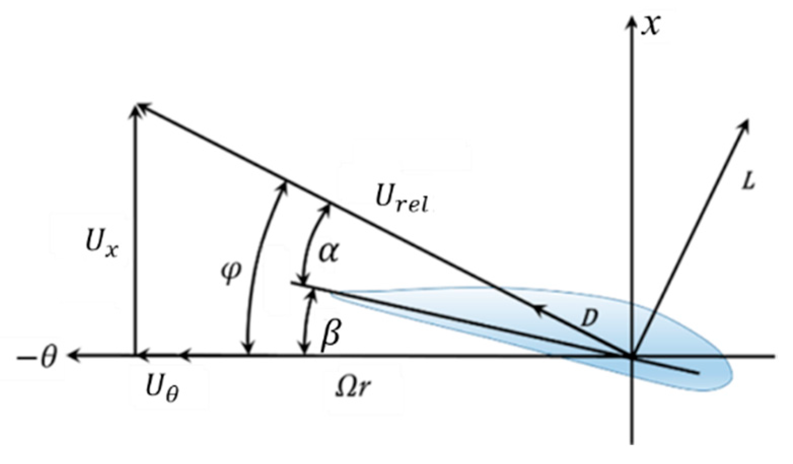
Full-scale blade-resolving simulations require lots of computational resources. Furthermore, flow features in the boundary layer on the blade surface were not the focus of the present work. Consequently, the actuator line model (ALM) proposed by Sørensen and Shen [33] was applied to model the interaction of the wind turbine blades with the wind in this work. In ALM, each turbine blade was treated as a rotating line source of body forces and divided into numerous blade elements, which were assumed as two-dimensional airfoils. Based on the local flow conditions sampled from the LES flow field and tabulated airfoil data, the blade-induced forces along the actuator line could be determined. A schematic of the lift and drag forces acting on a blade element and the local velocity relative to the rotating blade are displayed in Figure 1.
In Figure 1, is the local twist, is the angle between the local relative velocity and the rotating blade element, is the angle of attack, defined as , and is the magnitude of the local relative velocity, which is determined by
where and are the axial and tangential velocity components of the inflow wind at the blade element, respectively; is the rotational speed of the turbine rotor.
According to the local flow condition and the airfoil data, the aerodynamic force acting at each blade element can be calculated and expressed as
where is the air density, is the local chord length, is the blade element width, and are the lift and drag coefficients, respectively.
After calculating the aerodynamic force at each blade element, the equal and opposite force is projected smoothly onto the flow field as volumetric body forces that enter the momentum equation (i.e., term VI in Equation (2)). Commonly, a three-dimensional Gaussian is used as the projection function, and the body force at a certain location in the flow field is given by
where is the index number, is the aerodynamic force acting at the blade element , is the distance between the location and that of the airfoil element at . is a constant parameter that determines the projection width, it affects the numerical stability and impacts the aerodynamic performance of the wind turbine [32,35]. In this work, according to the results of the internal sensitivity studies, we chose as 5.0, about twice the grid size around the wind turbine, which is also a recommended value by Troldborg et al. [36].
2.3. Numerical Setup
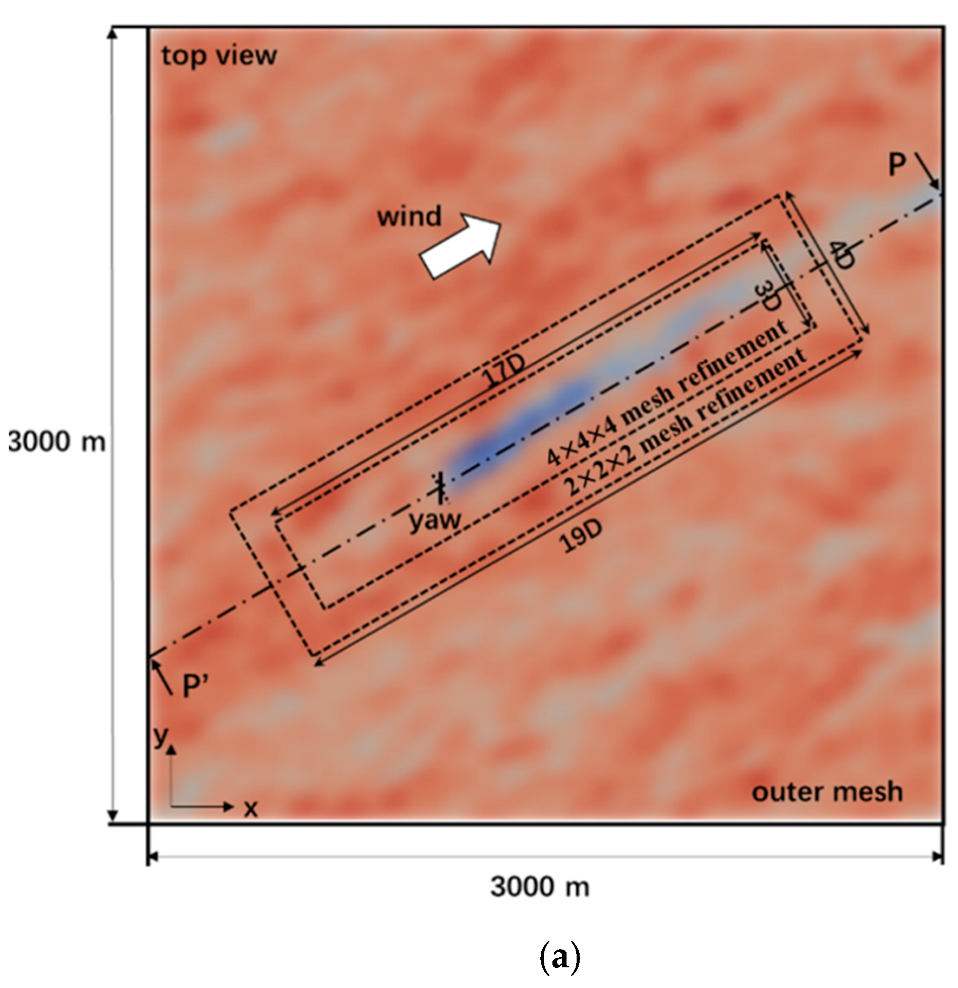
The entire simulation was divided into two stages. Firstly, a precursor simulation of a neutral boundary layer (NBL) flow without wind turbines was carried out to generate inflow conditions for the wind turbine wake simulation. As shown in Figure 2, the computational domain extends 3000 m × 3000 m × 1008 m and is divided uniformly into 250 × 250 × 84 grid points in the x, y, and z coordinate directions, respectively. In this simulation stage, all lateral boundaries were periodic, and a frictionless slip-wall boundary condition was applied at the upper boundary. Additionally, as mentioned above, both viscous and SGS effects are important at the bottom surface, implying that a sufficiently fine mesh is required to resolve the inner-layer structures near the rough boundary surface. To avoid such restriction, a surface model [37] was employed, in which, SGS and viscous stresses and temperature fluxes are lumped together, and the method has been widely employed in the simulations for the atmospheric boundary layers [38,39]. The surface aerodynamic roughness height in this work was set to 0.001 m, typical of the offshore conditions. The horizontal time-averaged wind speed at hub height was driven to 8 m/s from the southwest, instead of being aligned with the x-axis direction. By doing so, the generated turbulent structures can move more realistically in the computational domain without being trapped by the periodic boundaries. Overall, the setup was the same as that for the inflow condition in reference [32]; it has been validated before and represents a realistic scenario. The precursor simulation ran for 18,000 s at first to ensure reaching a quasi-steady condition. Then, it ran another 1000 s, and during that time, the relevant flow variables on the upstream boundary were stored at every time step, which would be enforced as the inflow boundary condition in the second simulation stage.
In the second stage, the wind turbine was immersed in the flow field and hence also referred to as “wind turbine wake simulation”. Note that boundary conditions of the second stage simulations are quite different from the precursor simulation. In particular, only the side boundaries are periodic; for the upstream boundary condition, as described above, it was specified using the saved turbulent data; on the downstream boundary, the velocity gradient was taken to be zero so that the generated turbulence structures in the precursor stage could enter the computational domain, and the turbine-induced wakes would be allowed to exit without cycling back. Moreover, we locally refined the mesh around the wind turbine and its wake so as to gain the resolution required to capture the wake structures. Specifically, the mesh refinement was carried out in two steps. In the first stage, the rectangular region had a length of 19D and a width of 4D, and the mesh cell size was divided in half of the background mesh, i.e., uniformly 6 m in all directions. In the second stage, the resolution of the inner zone with a length of 17D and a 3D width was further refined to 3 m cells. Details on the wind turbine position and the domain mesh are displayed in Figure 2.
The wind turbine used in this paper is the NREL 5 MW reference turbine including its baseline controller. This is a three-blade upwind turbine with a hub height of 90 m and a rotor diameter of 126 m. More details about it can be found in reference [40], which is publicly available. Note that in order to exclude wake displacements due to vertical momentum, no vertical tilt is applied to the turbine rotor. Although in fact there is a 5.0 shaft tilt to avoid the blade-tower collision.
To systematically investigate the yawing effect, four numerical simulations were carried out, in which yaw angles of the wind turbine are set to 0°, 10°, 20°, and 30°. The thrust coefficient of the yawed wind turbine in this study is defined as
where is the total force exerted on the wind turbine, is the air density, is rotor area, and is the mean incoming velocity at turbine hub height.
3. Numerical Results
The main characteristics of the simulated inflow condition are presented in Section 3.1. Then, the numerical results for wind turbine wake simulation under the non-yawed condition are validated in Section 3.2. In Section 3.3, turbine wake properties with different yaw angles are analyzed.
3.1. Inflow
In the precursor simulation, after the turbulent boundary layer flow reached a quasi-equilibrium state, we extracted the flow field data in the next 1000 s, and then, the statistical features of the inflow condition were obtained by taking the average of the sampled data.
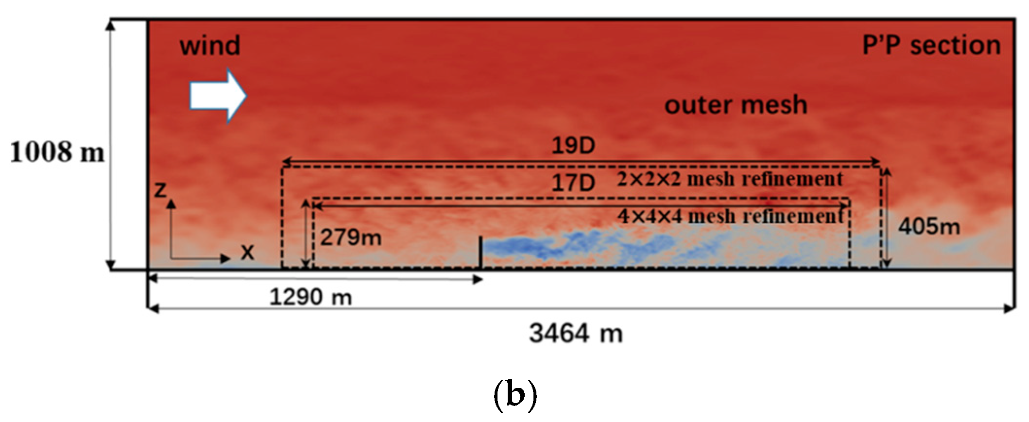
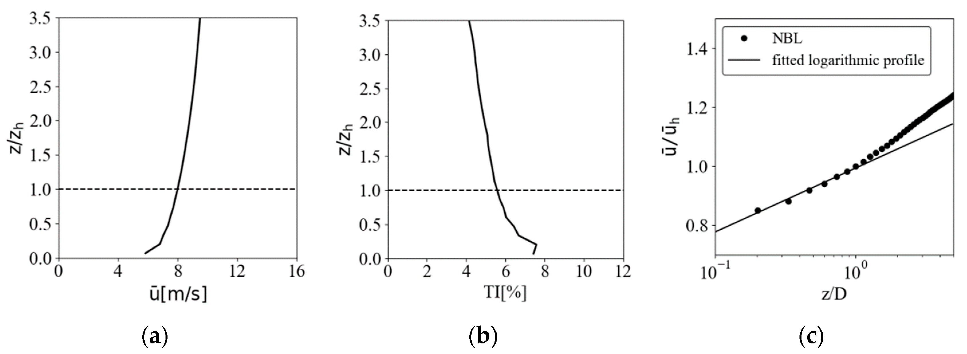
In Figure 3, the vertical profiles of the normalized streamwise inflow velocity and the streamwise turbulence intensity are shown. Specifically, the mean incoming wind speed and the turbulence intensity at hub height are about 8 m/s and 5.8%, respectively. Furthermore, to assess the simulated boundary layer flow, we plotted the measured streamwise velocity profile and the perfect logarithmic velocity profile on a semi-log scale, and as is displayed in Figure 3c, they are denoted by black dots and solid line, respectively. It can be seen from Figure 3c that below approximately 100 m, corresponding to the position of in the x label, the measured inflow velocity profile substantially satisfies the law of the wall scaling. This is an important feature to distinguish the neutral boundary layer (NBL) flow from other thermal stabilities, indicating that the desired inflow condition can be created well in the precursor simulation.
3.2. Validation of Numerical Model
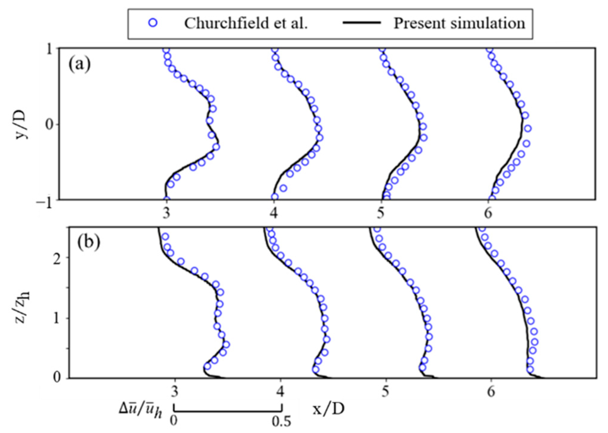
Next, we examine the accuracy of wind turbine wake simulation. The mean wake velocity deficits under the non-yawed condition are compared with the results from Churchfield et al. [32], which is widely accepted and cited. In their works, the wake flow features and aerodynamic performance of the NREL 5-MW wind turbine were investigated under the same inflow condition as the current simulation. Figure 4 compares the horizontal as well as vertical profiles of the normalized streamwise velocity deficit in the present work and that calculated by Churchfield et al., and a good agreement is found at different downwind locations.
Considering that in all numerical simulations in the present work, except for the yaw angle of wind turbines, other settings are the same, including the same computational domain, boundary conditions, inflow condition, time steps, etc. Therefore, according to the above comparisons, it is reasonable to acknowledge that the LES results of the wind turbine wake simulations with different yaw angles are accurate.
3.3. Wake Deflection and Velocity Deficit
In this section, we present the results from large-eddy simulations of the wake flow behind a wind turbine at different yaw angles. Emphasis is placed on wake deflection and velocity deficit distribution, as they are the key characteristics of the yawed turbine wake and are important for building analytical models.
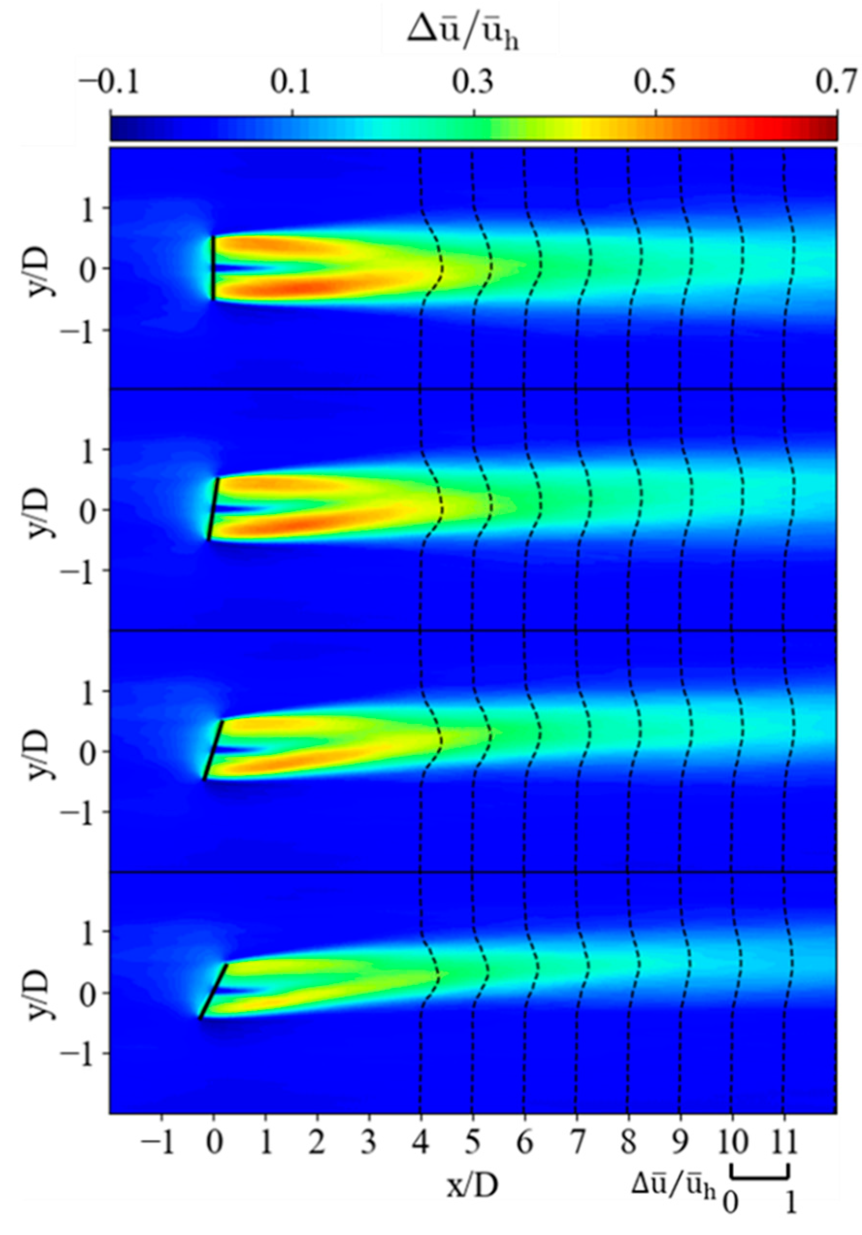
Figure 5 shows contour plots of the mean streamwise velocity deficit in the horizontal cross section at turbine hub height for γ = 0°, γ = 10°, γ = 20°, and γ = 30°. As expected, the wake region behind the yawed wind turbine moves away from the centerline with increasing downstream distance, and as the yaw angle increase, the wake deflection becomes more intense. In addition, for larger yaw angles, due to the decreased effective rotor area facing the incoming wind, both the momentum extracted from the ambient airflow and the thrust coefficient of the wind turbine are reduced; further, the wake width and velocity deficit in the wake region are also decreased accordingly. In each subgraph, the black dashed lines represent the mean streamwise velocity deficit profiles, which are found approximately satisfy the Gaussian distribution after some downstream distance, whether the wind turbine is yawed or not. Such wake behavior has also been reported in previous studies [41,42].
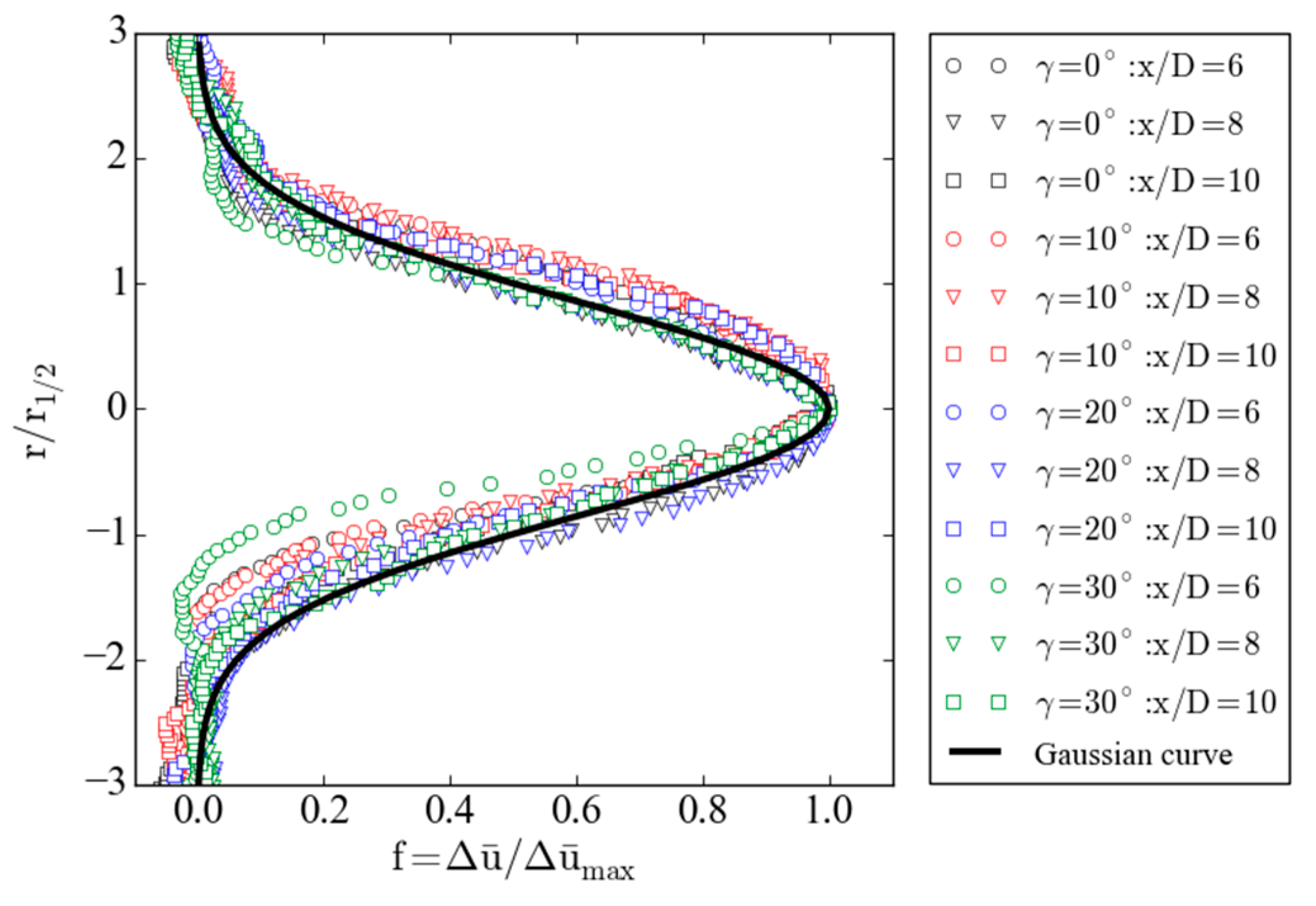
In order to further examine the self-similar Gaussian characteristics for the streamwise velocity deficit profiles at different yaw angles, the mean velocity deficit in the horizontal hub height plane, normalized by its maximum, is plotted as a function of the normalized radial distance from the wake center, as displayed in Figure 6. Note that the wake center is defined as the point where the velocity deficit is the maximum at each downwind location, is the half-width of the wake, which is the distance between the wake center and the point where the velocity deficit is half of the maximum value. From Figure 6, it is clear that the normalized velocity deficit profiles at different downwind distances collapse onto a single Gaussian curve, except near the edge of the wake where the shear is strong. Therefore, it is reasonable to take a Gaussian distributed shape for the velocity deficit profile in the far-wake region downstream of a yawed wind turbine.
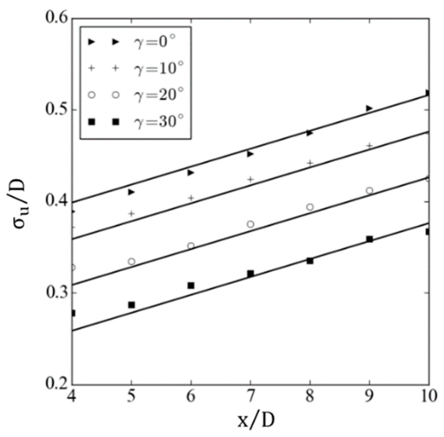
Additionally, properly estimate the variation of wake width is also critical for predicting the wake velocity distribution. To quantify the wake expansion, the standard deviation (indicated as in the y label of Figure 7) of the Gaussian curve fitted to the velocity deficit profile in the wakes was used as the characteristic wake width, as conducted by Abkar et al. [20,40] and Qian et al. [26,27]. Then, the normalized standard deviation was plotted against the normalized downstream distance, as presented in Figure 7. The result suggests that the wake width expands, approximately, linearly in the far-wake region, consistent with the observation of Xie et al. [41] and Bastankhah et al. [43]. Moreover, as indicated by the fitted lines, we can also find that the wake expansion rate is roughly the same for different yaw angles. This is because the wake recovery in the far-wake region is mainly affected by the incoming wind. The wind turbine properties, for example, thrust coefficient and yaw angle, only impact the flow behavior in the near-wake region [25]. In particular, for the current study, although the yaw angles are different, the wind turbines operate in the same inflow condition; thus, their wakes have almost the same expansion rate.
4. A New Wake Model and Validation
In Section 4.1, based on the assumptions of a Gaussian distribution for streamwise velocity deficit and a top-hat shape for skew angle, a new analytical model is derived to predict the wake center trajectory and mean streamwise velocity downstream of a yawed wind turbine. Subsequently, through comparison with wind tunnel tests and numerical simulations, the effectiveness of the proposed model is validated in Section 4.2.
4.1. Model Derivation
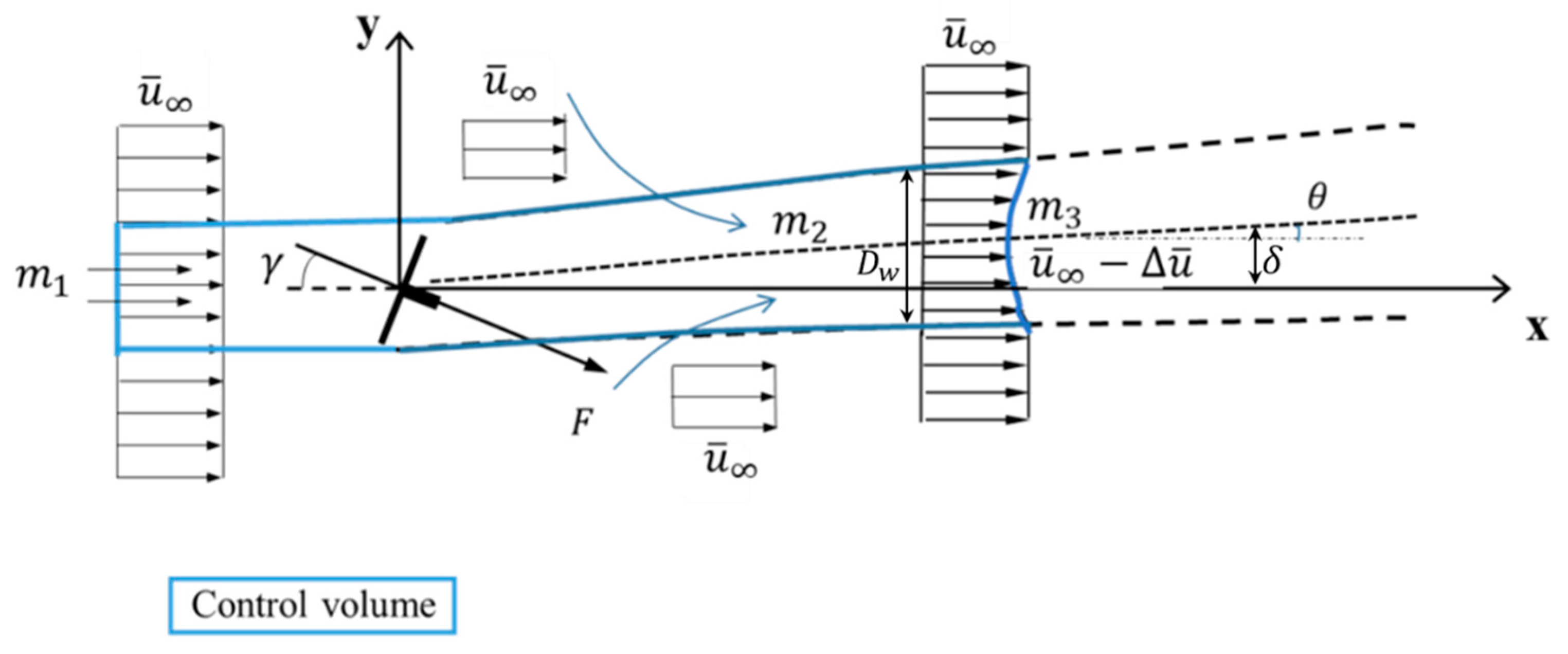
Similar to the derivation process of Jiménez et al. [9], we first constructed a control volume around the yawed wind turbine and its wake region, as shown in Figure 8, colored by the blue solid line, where denotes the wake center deflection magnitude, represents the yaw angle of the wind turbine, and is the wake skew angle, which is induced by the lateral force and defined as the inclined angle between the wake flow and the time-averaged incoming wind vector. Note that in Figure 8 and the remainder of this paper, is positive in the clockwise direction, and is positive in the counter-clockwise direction, from the top view. In addition, is the mass crossing the inlet, and denotes the mass of the incoming wind that enters the control volume through the lateral contour. For the calculation of and , both correspond to the unperturbed inflow velocity . is the mass through the wake cross section and is expressed as
In order to obtain the value of , it is necessary to specify the wake boundary. As illustrated in Section 3.3, the streamwise velocity deficit profiles in the wakes can be acceptably represented by self-similar Gaussian shapes after a certain downwind distance. As is well known, for the standard Gaussian function, the confidence interval equals 99.7% for (where is the standard deviation), i.e., approximately 99.7% of the values fall in that range. Therefore, in this work, the wake boundary is defined as
where is the standard deviation of the Gaussian curve fitted to the velocity deficit profile in the wakes.
According to the law of mass conservation, it yields
Furthermore, since the self-similarity assumption only applies to the far-wake region, where the pressure has recovered to the atmospheric free level. Hence, in the momentum equation, the turbine-induced force is the only item to balance the momentum flow rate across the boundaries.
The direction of the turbine-induced force is supposed to be perpendicular to the rotor plane, and its value is given by
where is the thrust coefficient, defined in Equation (11); is the rotor area, and is the unperturbed incoming wind speed.
Decomposing Equation (15) in streamwise and spanwise directions, respectively. Then, the two following equations can be obtained:
where is the streamwise velocity in the wake region, defined as
As the skew angle is small enough, therefore
Inserting Equations (14), (16) and (21) into Equation (17) gives
Interestingly, if substitute with , it is not difficult to find that Equation (22) is the same as the momentum equation for the non-yawed turbine wake derived by Bastankhah et al. [43], i.e., Equation (A1) in Appendix A. Furthermore, in the far-wake region of a yawed wind turbine, the self-similar Gaussian distribution for velocity deficit profile has been validated, and the wake width is found to increase linearly with the downstream distance. These two points are exactly the basic of the non-yawed wake model proposed by Bastankhah et al. [43]. Moreover, considering that in the same inflow condition, the wake expansion rate is around the same for different yaw angles. Consequently, incorporating the yawing effect into the analytical model for the non-yawed wind turbine [43] and using the modified version to predict the yawed turbine wakes is reasonable.
From the above analysis, analogous to Equations (A3) and (A4) in Appendix A, the normalized streamwise velocity deficit at each downstream location behind a yawed turbine can be expressed as
where denotes the maximum normalized velocity deficit occurring at the center of the wake, and is the radial distance from the wake center. is the normalized standard deviation of the Gaussian-fitted velocity deficit profile; it is written by
where is the wake growth rate, its value is specified in the input; is a model parameter, corresponding to the value of as approaches 0. With reference to Bastankhah et al. [43] and Frandsen et al. [44], and considering the yawing effect is expressed as
The term in the square root of Equation (24) may be negative, especially under heavy load cases with large thrust coefficients, which can lead to calculation errors. Therefore, following the work of Qian et al. [26], Taylor expansion is performed on Equation (24) to obtain its first-order approximation, and then, the new form is applied to estimate the maximum velocity deficit in yawed turbine wakes.
According to Equations (19), (23) and (28), the normalized wake velocity in the yawed wake region is given by
Apart from the streamwise velocity that is modeled by a straight wake generated by an equivalent non-yawed turbine, the wake deflection is also a key characteristic for the yawed turbine wake, which is induced by the lateral force. Hence, the spanwise momentum equation will be analyzed in the following.
First, the skew angle should be considered, as it is the derivative of the wake deflection. For the sake of simplicity, the skew angle was assumed to have a top-hat shape in this work, i.e., at each downstream cross section, is constant within the defined wake boundary. Based on this assumption and rearranging Equation (18), the wake skew angle can be found as follows:
Inserting Equation (29) into Equation (30) and calculating the integration based on the assumed wake boundary yield
Note that Equation (31) is only applicable to the far-wake region, as the self-similar assumption for the velocity deficit profile is applied in its derivation process.
For the skew angle in the near-wake region, it can be estimated based on the work of Coleman et al. [45] that
Obviously, in order to correctly use Equations (31) and (32), the boundary between the far-wake region and the near-wake region should be reasonably specified. Here, we define this position as and determine mathematically that the wake skew angle has the same value at . Specifically, by making Equations (31) and (32) equal, the normalized standard deviation at is obtained
Further, Equation (25) results in the following:
Similar to the discussion on the skew angle, the calculation of wake deflection is also divided into two parts.
In the near-wake region, the normalized wake deflection, indicated by , is assumed to vary linearly with the downstream distance:
In the far-wake region, the wake deflection can be obtained by integrating the skew angle in Equation (31), from the initial far wake location . The value of wake deflection at is used as the integration constant.
For completeness, the final expression of the equation used to predict the streamwise velocity behind a yawed wind turbine is written as follows:
where and are spanwise and vertical coordinates, respectively, is the wake center deflection at each downstream location, and is the turbine hub height.
4.2. Model Validation
To validate the new proposed model, its predictions are firstly compared to wind tunnel measurements of Bastankhah et al. [18] and other commonly used wake models shown in the Appendix B, Appendix C and Appendix D. The experiments were carried out in a neutrally turbulent atmospheric boundary layer, the incoming wind speed and the turbulence intensity at hub height are about 4.88 m/s and 7%, respectively. Furthermore, the thrust coefficients of the wind turbine at different yaw angles in the experiments are summarized in Table 1.
In order to use the analytical models, input parameters should be determined in advance. Specifically, in the Bastankhah–Porté-Agel model [25], and (in Appendix C) are set to 0.022; and values of , are chosen 0.58 and 0.077, respectively, to fit the experimental data. For comparison, in the new proposed model is also taken to be 0.022, while in the model of Jimenez et al. [9], (in Appendix B) is set to 0.05, as the surface roughness in the experiment is on the order of on-shore cases. For the Qian–Ishihara model [26], as described in Appendix D, since its parameters are modeled as a function of thrust coefficient and ambient turbulence intensity, no specificity is required.
Note that because of the difference in the definition of thrust coefficient, when applying the Jimenez model and the Qian–Ishihara model, should be replaced with in the calculations.
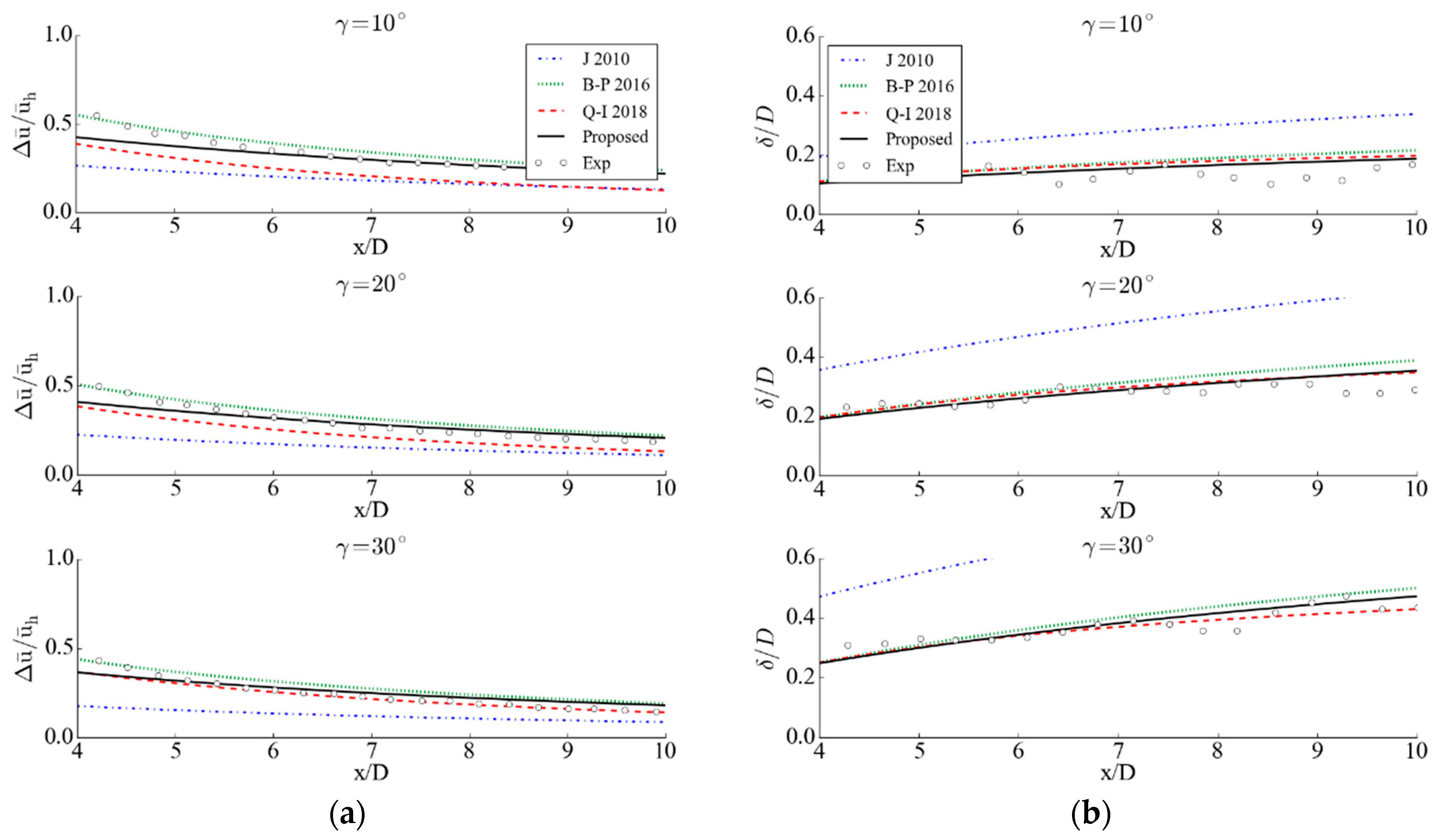
Figure 9 shows the variation of the maximum velocity deficit and the wake center deflection with respect to the downstream distance for different yaw angles, where the x-axis represents the normalized distance from the wind turbine, and the experimental data are shown by white circles. As displayed in Figure 9a, the Bastankhah–Porté-Agel model can well predict the maximum velocity deficit. With the wake propagating downstream, good consistency is also observed between the experimental data and the predictions of the new proposed model, especially after 5D downstream distance. The Jimenez model greatly underpredicts the maximum velocity deficit and overestimates the wake deflection for all yaw angles. In the predictions of the Qian–Ishihara model, the maximum velocity deficits are also underestimated, but good estimations on the wake center deflection are found, particularly for the cases of γ = 20° and γ = 30°. In addition, as can be seen in Figure 9b, the wake center deflection, obtained from the Bastankhah–Porté-Agel model and the new proposed model, are both in good agreement with the experiment. In more detail, the Bastankhah–Porté-Agel model tends to slightly overpredict the deflection magnitude, while the new proposed model provides better results.
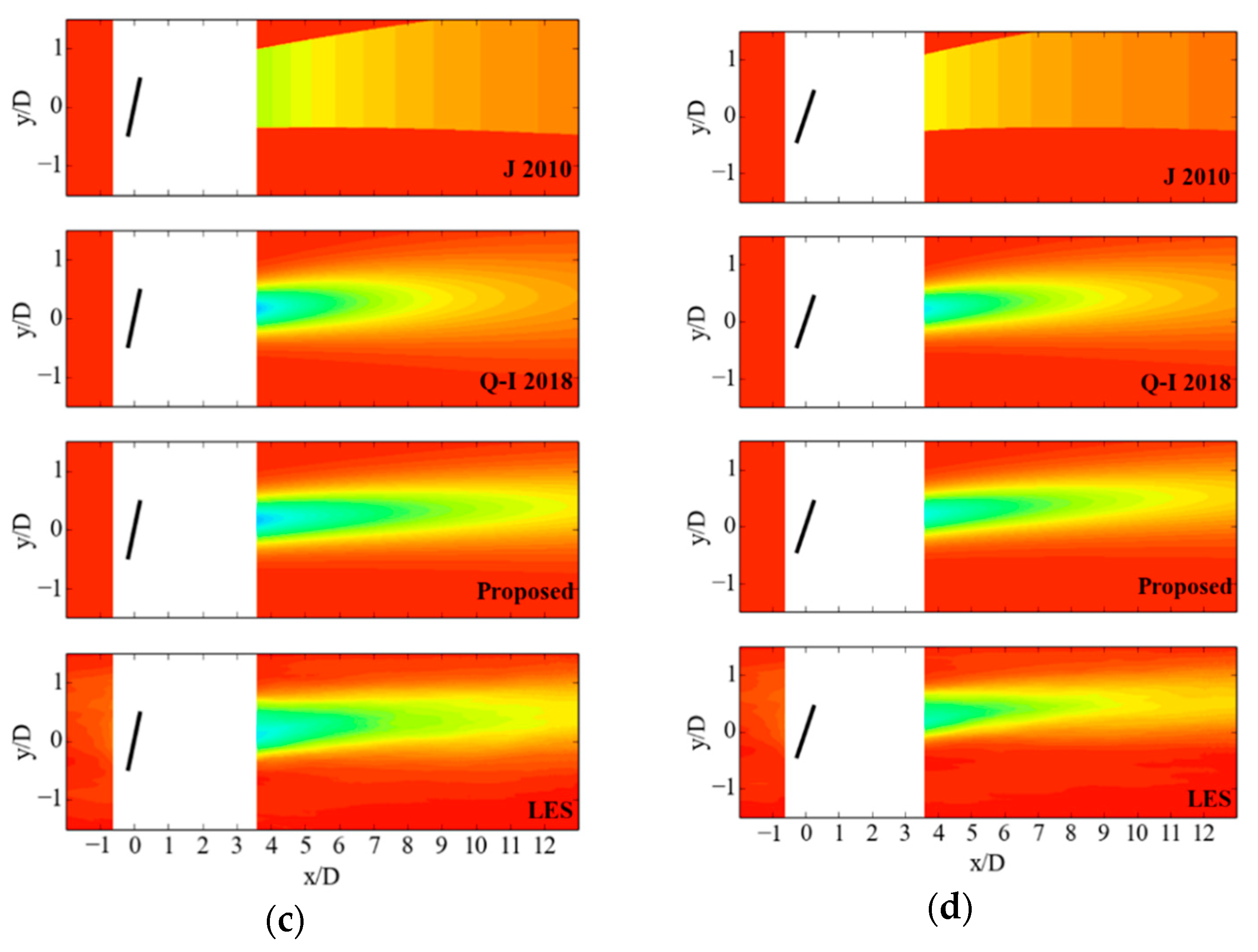
Besides the comparison with wind tunnel tests for a model wind turbine, in the following, model predictions are also compared to the large-eddy simulations for a utility-scale wind turbine. The numerical setup of the test cases and the inflow condition have been illustrated in Section 2.3 and Section 3.1, respectively. The input parameters of the analytical models are set as follows: for the new proposed model, the value of can be found from the LES data in Figure 7, about 0.02; in the Jimenez model, is again taken to be 0.05; for the Qian–Ishihara model, as mentioned above, its parameters are calculated by and . Since the input parameters of the Bastankhah–Porté-Agel model are difficult to specify accurately, especially for and , its predictions are not drawn here.
Figure 10 presents the hub-height contour plots of the mean streamwise velocity obtained from the numerical simulations and predictions of analytical models. As seen, only the new proposed model can well capture the wake characteristics for different yaw angles. The Jimenez model greatly deviates from the numerical results, and the possible reason for the departure is the top-hat distribution assumption for the velocity deficit profile that it adopted. Furthermore, the Qian–Ishihara model is observed to underestimate the velocity deficits in yawed wakes, in particular, for γ = 10° and γ = 20°, which may cause large mistakes in the real-world engineering projects.
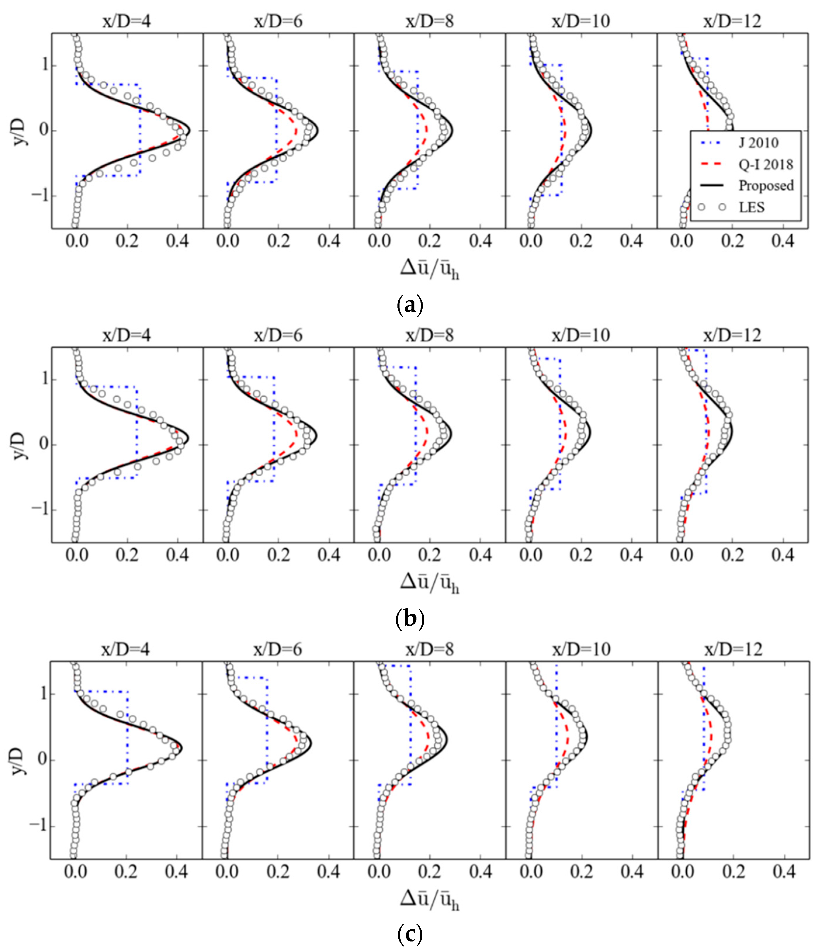
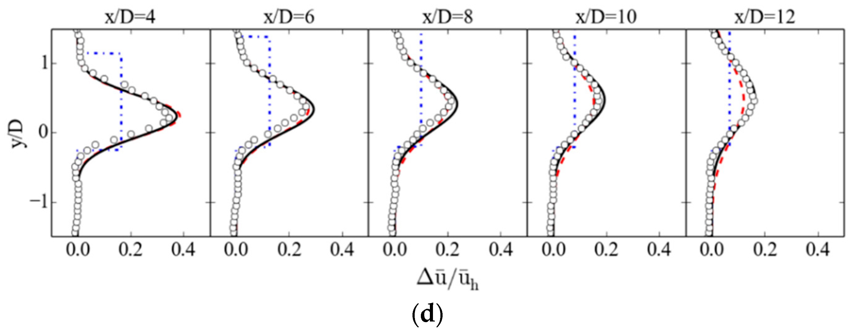
In order to obtain a more quantitative comparison, horizontal profiles of the mean velocity deficit predicted by different analytical models and the LES results are plotted in Figure 11. As shown, the results obtained from the new proposed model are in acceptable agreement with the LES data; in other words, the new model can thoroughly capture the variation of the wake deflection magnitude against the downstream distance and the distribution of mean velocity deficit. The Jimenez model incorrectly overestimates the wake center deflection, and further, the lateral distribution of the velocity deficit is also quite different from the real situation. Specifically, is underpredicted in the wake center region but overestimated near the edge of the wake. Additionally, the predictions of the Qian–Ishihara model are found to underestimate the velocity deficit in the wakes for γ = 0°, γ = 10° and γ = 20°, although they yield reasonable wake deflections.
From the above analysis, it can be concluded that, compared with the wind tunnel tests, both the Bastankhah–Porté-Agel model and the new proposed model show good performance in estimating the wake center position and the maximum velocity deficit in yawed turbine wakes. However, there are many parameters in the Bastankhah–Porté-Agel model, and in order to reasonably estimate their values, especially the parameters of and used to determine the onset of the far-wake region, a large number of numerical simulations or wind tunnel experiments are required. Evidently, this prevents the Bastankhah–Porté-Agel model from being widely used.
Different from the Bastankhah–Porté-Agel model, in the analytical wake model proposed by Qian and Ishihara, empirical expressions of the model parameters are given as a function of ambient turbulence intensity and thrust coefficient, which enables the model to be applied under various conditions. However, in terms of predicting wake features, the Qian–Ishihara model exhibits biases toward underestimating the streamwise velocity deficit in the wake region, particularly in the cases with small yaw angles.
The largest deviation from the experimental data and the LES results is found in the prediction of the Jimenez model. It overestimates the wake deflection and underestimates the velocity deficit in the center of the wake. This can be attributed to the assumption of the top-hat distribution for the velocity deficit. Compared to the velocity deficit profiles for the yawed wind turbine as presented in Figure 6, it is clear that the top-hat assumption is unrealistic.
The newly proposed analytical model can provide accurate predictions on the wake characteristics of the wind turbine at different yaw angles. We only need to reasonably estimate the wake growth rate.
5. Extension to Predict Transverse Velocity
In a wind farm, the cross flow induced by the yawed wind turbine continues to exist after the combination of wakes, causing the “secondary steering” [28,29], which can affect the power production and has important implications for wind plants’ controller design. Therefore, it is necessary to establish models for predicting the transverse velocity in the yawed turbine wakes. However, compared with the widely studied streamwise velocity, the transverse velocity has received less attention in previous studies. Moreover, considering the complexity of the transverse velocity distribution, directly modeling it is difficult. Fortunately, there is a clear relationship between the wake skew angle and the wake velocity components, which provides another possible solution for the transverse velocity prediction under yawed conditions.
To this end, we first study features of the wake skew angle, as illustrated in Section 4.1, which is defined as the inclination angle of the wake velocity vector with respect to the mean inflow direction; thus,
where and are the wake velocity components along the streamwise and spanwise directions, respectively.
The skew angle is small with the approximation of , the Equation (38) can therefore be rewritten as
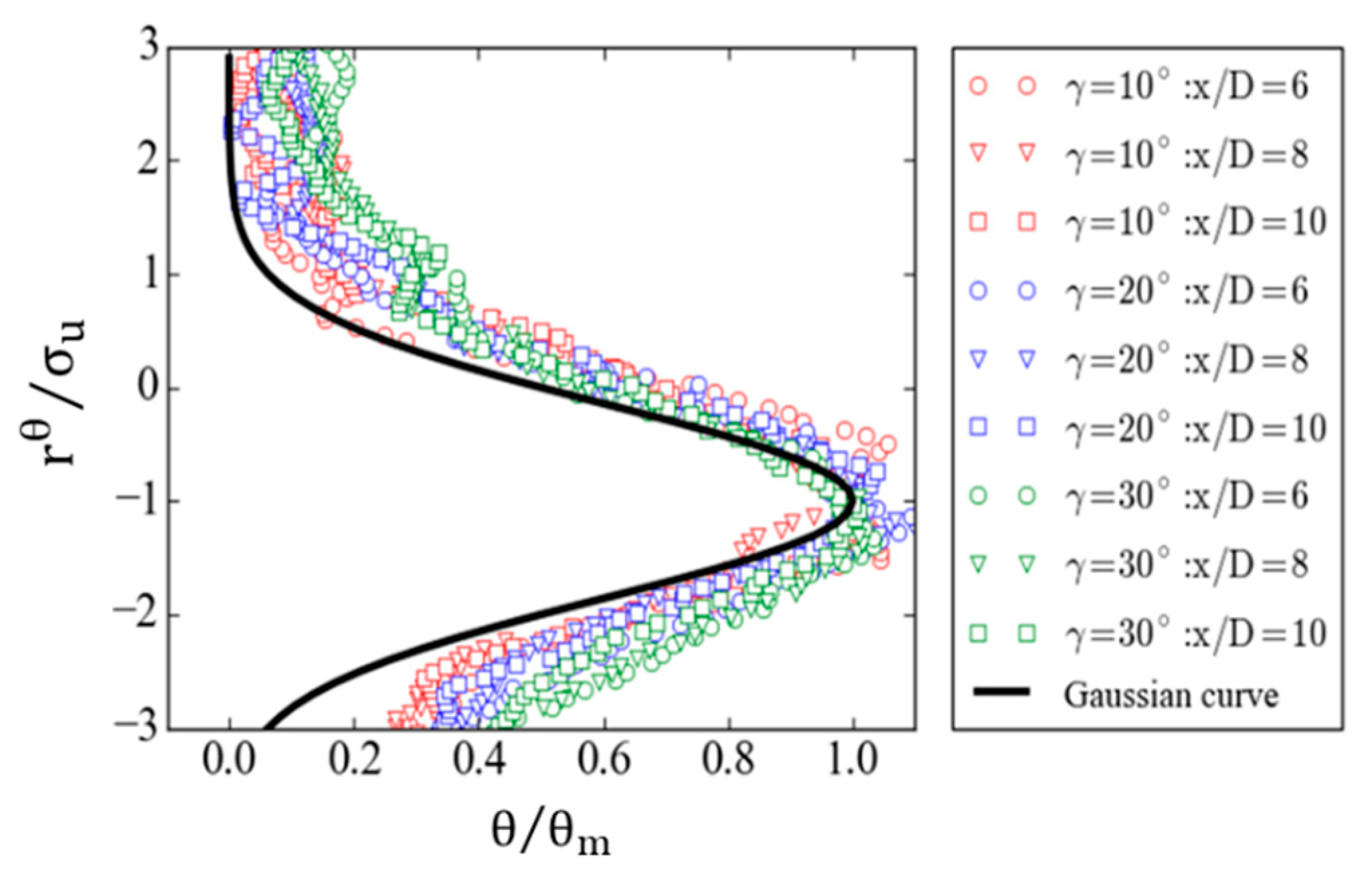
Referring to the study of Bastankhah et al. [25], apart from the streamwise velocity deficit profile, the lateral variation of the skew angle at hub height in the far-wake region of a yawed wind turbine can also be approximated with a self-similar Gaussian distribution. Furthermore, as apparent in Figure 12, the maximum skew angle does not occur at the wake center but on the one side of the wake, roughly at , where is the lateral distance from the wake center position, and is the standard deviation of the Gaussian-fitted velocity deficit profile.
From the above analysis, the skew angle distribution in yawed turbine wakes can be approximated by
where denotes the wake center deflection at each downstream location.
Based on the model derivation process in Section 4.1 in which, to avoid complicated integration calculations, a top-hat shape is assumed for the lateral skew angle profile, combined with the momentum equation in the spanwise direction, Equation (31) is derived to determine the skew angle in the yawed wake region. Note that, as the skew angle is considered to be constant at each downstream cross section in that process, the result by Equation (31) is actual an average value of the skew angle within the defined wake boundary. For better distinction, in Equation (31) is referred to by hereafter.
Although the detailed flow characteristic is neglected, with a good estimation of the wake growth rate, Equation (36) based on a top-hat distribution for the skew angle can still capture the wake deflection downstream of a yawed turbine, as shown in Figure 9b. However, to accurately predict the transverse velocity in the yawed wakes, a more realistic description of the lateral skew angle profile is required. In the above analysis, it has been proved that the skew angle profiles in the spanwise direction can be represented by self-similar Gaussian distribution. Therefore, as long as the maximum value of skew angle at each downwind location is given, the above goal can be achieved.
Based on the existing modeling results, we plan to adopt the following strategies: (1) solve Equation (31) at first, to obtain an average value of the skew angle at each downstream position; (2) redistribute the skew angle at a Gaussian shape. Specifically, at each downwind location behind a yawed turbine, establish a Cartesian coordinate system with the origin at the wake center and then set the average value of Equation (40) within the defined wake boundary to be equal to the result by Equation (31).
The maximum value of skew angle with a Gaussian shape can be therefore obtained.
To reemphasize, here, is the skew angle value calculated by Equation (31).
Next, by inserting Equations (40) and (42) into Equation (39), the transverse velocity in yawed turbine wakes can be determined as follows:
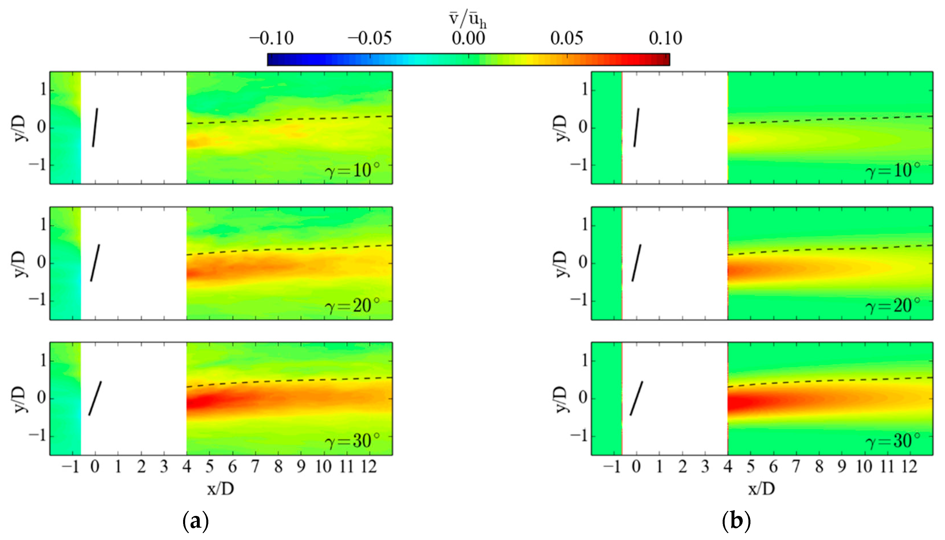
To validate the proposed model, numerical simulations for the yawed wind turbine described in Section 2.3 are used once again as test benchmarks. Figure 13 compares the contours of the transverse velocity at hub height for γ = 10°, γ = 20°, and γ = 30°. From the figure, one can clearly observe an asymmetric distribution for the transverse velocity with respect to the wake center trajectory denoted by the black dashed line. The proposed model is found to be in excellent agreement with the LES results.
6. Conclusions
In the present work, a series of numerical simulations were performed with the SOWFA tool, to investigate the wake characteristics at different yaw angles. Emphasis was placed on the wake deflection and the wake velocity distribution. The results suggest that with increasing yaw angles, the wake deflection increases as expected. Additionally, the self-similarity for the streamwise velocity deficit profiles in the far-wake region was assessed. The wake width, represented by the standard deviation of the Gaussian-fitted velocity deficit profile, is found to expand linearly against the downstream distance and has approximately the same growth rate for different yaw angles. This is due to the fact that the velocity recovery in the far-wake region is mainly affected by the incoming flow properties.
Based on the numerical simulation results and theoretical analysis, an extension of the classical Bastankhah non-yawed wake model [43] was made. Combined with the consideration of the wake deflection due to yaw, a new analytical model for predicting the wake center trajectory and mean streamwise velocity in the far-wake region of a yawed wind turbine was developed. Furthermore, according to a relationship between the skew angle and wake velocity components, the proposed model was further extended to incorporate the prediction of the transverse velocity at hub height. This is very meaningful, as the transverse velocity plays an important role in capturing the secondary wake steering effect crucial to yaw angle control.
By comparing with the results from wind tunnel tests, numerical simulations, and other common analytical wake models, the new proposed model is found to be able to accurately predict the key wake characteristics under yawed conditions, including the wake deflection, streamwise velocity, and transverse velocity on the hub-height plane. More importantly, the new proposed model is simple in form—only one parameter (i.e., the wake growth rate) needs to be specified apart from the basic information about the wind turbine and the ambient inflow condition. This makes it easy to be used in practice. In the future, we plan to apply the proposed model over a small-scale wind farm to investigate the effectiveness of the yaw angle control strategy or seek the best yaw angle distribution for mitigating wake effects.
Author Contributions
The paper was a collaborative effort among the authors. D.-Z.W. performed the modeling, designed the structure, and wrote the paper. D.-C.W. supervised the related work. N.-N.W. polished the language of the paper. All authors have read and agreed to the published version of the manuscript.
Funding
This research was funded by the National Key Research and Development Program of China (2019YFB1704200 and 2019YFC0312400), National Natural Science Foundation of China (Grant No. 51879159).
Institutional Review Board Statement
Not applicable.
Informed Consent Statement
Not applicable.
Data Availability Statement
Not applicable.
Acknowledgments
Thanks to the researchers from the National Renewable Energy Laboratory (NREL) for providing the related open-source code: Simulator for Wind Farm Applications (SOWFA). This work was supported by the National Key Research and Development Program of China (2019YFB1704200 and 2019YFC0312400), National Natural Science Foundation of China (Grant No. 51879159), to which the authors are most grateful.
Conflicts of Interest
The authors declare no conflict of interest.
Appendix A. Wake Model for Non-Yawed Wind Turbines by Bastankhah and Porté-Agel
By applying conservation of mass and momentum for the control volume around the wind turbine, the simplified momentum equation, neglecting the viscous and pressure terms, for the non-yawed turbine wake, can be expressed as follows:
where is the turbine induced force, determined as
Furthermore, according to the assumption of the Gaussian-like shape for the velocity deficit profile, the following equation can be obtained:
where denotes the maximum velocity deficit at each , describes the Gaussian-like velocity deficit profile.
By inserting Equations (A2) and (A3) into Equation (A1), and through solving, the maximum velocity deficit can be calculated as follows:
where is the normalized standard deviation of the Gaussian-fitted velocity deficit profile, which is assumed to increase linearly with the downstream distance.
where is the wake growth rate, is the value of when is closed to 0, it can be estimated by comparison with the Frandsen model [44], expressed as
Appendix B. Jiménez Model for Yawed Wind Turbine Wakes
Based on the top-hat assumption for the velocity deficit and skew angle profiles, Jimenez et al. [9] built a simple model to describe the yawed turbine wake, in which, the skew angle is determined as
Appendix C. Bastankhah–Porté-Agel Model for Yawed Wind Turbine Wakes
On the basis of the self-similarity for both velocity deficit and skew angle profiles, along with the budget study of RANS equations, Bastankhah and Porté-Agel [25] proposed a Gaussian model for the yawed turbine wakes.
In this model, analogous with coflowing jet, the near-wake region behind a yawed turbine is modeled as a potential core, and its length can be determined as follows:
where and are model parameters, their estimations rely heavily on numerical simulations or wind tunnel measurements.
The wake skew angle in the near-wake region is assumed constant, given by
In the near-wake region, the wake deflection can be estimated by
In the far-wake region where , the wake deflection is expressed as follows:
where and are the wake growth rate in lateral and vertical directions, respectively. and are the corresponding wake widths, can be found by
Furthermore, the normalized streamwise velocity deficit in the far-wake region is written as
Appendix D. Qian–Ishihara Model for Yawed Wind Turbine Wakes
In the model proposed by Qian and Ishihara [26], the estimation of the wake skew angle is divided into two parts. In particular, in the near-wake region, the skew angle is given by
where is the thrust coefficient, which has the same form as Equation (A9) in Appendix B.
In the far-wake region, the wake skew angle is expressed as follows:
where is the normalized standard deviation, which is assumed to increase linearly with the downstream distance,
where and are the parameters, which are modeled as functions of the ambient turbulence intensity and thrust coefficient of the wind turbine.
By equating Equations (A18) and (A19), the onset location for the far-wake region can be determined as follows:
The wake center deflection for can be estimated by
In the far-wake region where , the wake deflection is found by integrating Equation (A19) along , from .
Based on the Gaussian-like shape for the velocity deficit profiles, the velocity distribution at each downwind distance behind a yawed wind turbine is expressed as
where represents the distance from the wake center, and is the maximum velocity deficit at each , which can be calculated by:
Additionally, this analytical model can also provide a prediction of the turbulence intensity distribution in yawed turbine wakes. However, as it is out of the scope of the current study, the relevant content is not given here.
References
- Barthelmie, R.J.; Pryor, S.C.; Frandsen, S.T.; Hansen, K.S.; Schepers, J.G.; Rados, K.; Schlez, W.; Neubert, A.; Jensen, L.E.; Neckelmann, S. Quantifying the impact of wind turbine wakes on power output at offshore wind farms. J. Atmos. Ocean. Technol. 2010, 27, 1302–1317. [Google Scholar] [CrossRef]
- Kim, S.H.; Shin, H.K.; Joo, Y.C.; Kim, K.H. A study of the wake effects on the wind characteristics and fatigue loads for the turbines in a wind farm. Renew. Energy 2015, 74, 536–543. [Google Scholar] [CrossRef]
- Storey, R.; Norris, S.; Cater, J. Large eddy simulation of wind events propagating through an array of wind turbines. In Proceedings of the World Congress on Engineering 2013, London, UK, 3–5 July 2013; Volume III. [Google Scholar]
- Adaramola, M.S.; Krogstad, P.-Å. Experimental investigation of wake effects on wind turbine performance. Renew. Energy 2011, 36, 2078–2086. [Google Scholar] [CrossRef]
- Dilip, D.; Porté-Agel, F. Wind Turbine Wake Mitigation through Blade Pitch Offset. Energies 2017, 10, 757. [Google Scholar] [CrossRef]
- Lee, J.; Son, E.; Hwang, B.; Lee, S. Blade pitch angle control for aerodynamic performance optimization of a wind farm. Renew. Energy 2013, 54, 124–130. [Google Scholar] [CrossRef]
- Bartl, J.; Muhle, F.; Schottler, J.; Sætran, L.; Peinke, J.; Adaramola, M.; Holling, M. Wind tunnel experiments on wind turbine wakes in yaw: Effects of inflow turbulence and shear. Wind Energy Sci. 2018, 3, 329–343. [Google Scholar] [CrossRef] [Green Version]
- Bartl, J.M.S.; Muhle, F.V.; Sætran, L.R. Wind tunnel study on power output and yaw moments for two yaw-controlled model wind turbines. Wind Energy Sci. 2018, 3, 489. [Google Scholar] [CrossRef] [Green Version]
- Jiménez, Á.; Crespo, A.; Migoya, E. Application of a LES technique to characterize the wake deflection of a wind turbine in yaw. Wind Energy 2010, 13, 559–572. [Google Scholar] [CrossRef]
- Fleming, P.; Gebraad, P.M.O.; Lee, S.; Wingerden, J.W.; Johnson, K.; Churchfield, M.; Michalakes, J.; Spalart, P.; Moriarty, P. Simulation comparison of wake mitigation control strategies for a two-turbine case. Wind Energy 2015, 18, 2135–2143. [Google Scholar] [CrossRef]
- Fleming, P.A.; Gebraad, P.M.O.; Lee, S.; van Wingerden, J.W.; Johnson, K.; Churchfield, M.; Michalakes, J.; Spalart, P.; Moriarty, P. Evaluating techniques for redirecting turbine wakes using SOWFA. Renew. Energy 2014, 70, 211–218. [Google Scholar] [CrossRef]
- Wang, J.; Foley, S.; Nanos, E.M.; Yu, T.; Campagnolo, F.; Bottasso, C.L.; Zanotti, A.; Croce, A. Numerical and experimental study of wake redirection techniques in a boundary layer wind tunnel. J. Phys. Conf. Ser. 2017, 854, 012048. [Google Scholar] [CrossRef]
- Miao, W.; Li, C.; Pavesi, G.; Yang, J.; Xie, X. Investigation of wake characteristics of a yawed HAWT and its impacts on the inline downstream wind turbine using unsteady CFD. J. Wind Eng. Ind. Aerodyn. 2017, 168, 60–71. [Google Scholar] [CrossRef]
- Gebraad, P.M.O.; Teeuwisse, F.W.; Wingerden, J.W.; Fleming, P.A.; Ruben, S.D.; Marden, J.R.; Pao, L.Y. Wind plant power optimization through yaw control using a parametric model for wake effects—A CFD simulation study. Wind Energy 2016, 19, 95–114. [Google Scholar] [CrossRef]
- Vollmer, L.; Steinfeld, G.; Heinemann, D.; Kühn, M. Estimating the wake deflection downstream of a wind turbine in different atmospheric stabilities: An LES study. Wind Energy Sci. 2016, 1, 129–141. [Google Scholar] [CrossRef] [Green Version]
- Howland, M.F.; Bossuyt, J.; Martínez-Tossas, L.A.; Meyers, J.; Meneveau, C. Wake structure in actuator disk models of wind turbines in yaw under uniform inflow conditions. J. Renew. Sustain. Energy 2016, 8, 043301. [Google Scholar] [CrossRef] [Green Version]
- Schottler, J.; Bartl, J.; Mühle, F.; Sætran, L.; Peinke, J.; Hölling, M. Wind tunnel experiments on wind turbine wakes in yaw: Redefining the wake width. Wind Energy Sci. 2018, 3, 257–273. [Google Scholar] [CrossRef] [Green Version]
- Bastankhah, M.; Porté-Agel, F. A wind-tunnel investigation of wind-turbine wakes in yawed conditions. J. Phys. Conf. Ser. 2015, 625, 012014. [Google Scholar] [CrossRef]
- Ozbay, A.; Tian, W.; Yang, Z.; Hu, H. Interference of wind turbines with different yaw angles of the upstream wind turbine. In Proceedings of the 42nd AIAA Fluid Dynamics Conference and Exhibit, New Orleans, LA, USA, 25–28 June 2012; p. 2719. [Google Scholar]
- Abkar, M.; Porté-Agel, F. Influence of atmospheric stability on wind-turbine wakes: A large-eddy simulation study. Phys. Fluids 2015, 27, 035104. [Google Scholar] [CrossRef] [Green Version]
- Wu, Y.T.; Porté-Agel, F. Atmospheric Turbulence Effects on Wind-Turbine Wakes: An LES Study. Energies 2012, 5, 5340–5362. [Google Scholar] [CrossRef]
- Howland, M.F.; Bossuyt, J.; Martinez-Tossas, L.A.; Meyers, J.; Meneveau, C. Wake Structure of Wind Turbines in Yaw under Uniform Inflow Conditions. arXiv 2016, arXiv:1603.06632. [Google Scholar]
- Chamorro, L.P.; Porté-Agel, F. Effects of thermal stability and incoming boundary-layer flow characteristics on wind-turbine wakes: A wind-tunnel study. Bound.-Layer Meteorol. 2010, 136, 515–533. [Google Scholar] [CrossRef] [Green Version]
- Gaumond, M.; Réthoré, P.E.; Ott, S.; Peña, A.; Bechmann, A.; Hansen, K.S. Evaluation of the wind direction uncertainty and its impact on wake modeling at the horns rev offshore wind farm. Wind Energy 2013, 17, 1169–1178. [Google Scholar] [CrossRef] [Green Version]
- Bastankhah, M.; Porté-Agel, F. Experimental and theoretical study of wind turbine wakes in yawed conditions. J. Fluid Mech. 2016, 806, 506–541. [Google Scholar] [CrossRef]
- Qian, G.W.; Ishihara, T. A New Analytical Wake Model for Yawed Wind Turbines. Energies 2018, 11, 665. [Google Scholar] [CrossRef] [Green Version]
- Qian, G.W.; Ishihara, T. A new Gaussian-based analytical wake model for wind turbines considering ambient turbulence intensities and thrust coefficient effects. J. Wind Eng. Ind. Aerodyn. 2018, 177, 275–292. [Google Scholar]
- Fleming, P.; Annoni, J.; Churchfield, M.; Martinez-Tossas, L.A.; Gruchalla, K.; Lawson, M.; Moriarty, P. A simulation study demonstrating the importance of large-scale trailing vortices in wake steering. Wind Energy Sci. 2018, 3, 243–255. [Google Scholar] [CrossRef] [Green Version]
- Martínez-Tossas, L.A.; Annoni, J.; Fleming, P.A.; Churchfield, M.J. The aerodynamics of the curled wake: A simplified model in view of flow control. Wind Energy Sci. 2019, 4, 127–138. [Google Scholar] [CrossRef] [Green Version]
- Shapiro, C.R.; Gayme, D.F.; Meneveau, C. Modelling yawed wind turbine wakes: A lifting line approach. J. Fluid Mech. 2018, 841, R1. [Google Scholar] [CrossRef] [Green Version]
- Bay, C.; King, J.; Fleming, P.; Mudafort, R. Unlocking the Full Potential of Wake Steering: Implementation and Assessment of a Controls-Oriented Model; Technical Report; National Renewable Energy Lab. (NREL): Golden, CO, USA, 2019.
- Churchfield, M.J.; Lee, S.; Michalakes, J.; Moriarty, P.J. A numerical study of the effects of atmospheric and wake turbine dynamics. J. Turbul. 2012, 13, N14. [Google Scholar] [CrossRef]
- Sørensen, J.N.; Shen, W.Z. Numerical modeling of wind turbine wakes. J. Fluids Eng. 2002, 124, 393–399. [Google Scholar] [CrossRef]
- Smagorinsky, J. General circulation experiments with the primitive equations. Mon. Weather Rev. 1963, 91, 99–164. [Google Scholar] [CrossRef]
- Stevens, R.J.A.M.; Martínez-Tossas, L.A.; Meneveau, C. Comparison of wind farm large eddy simulations using actuator disk and actuator line models with wind tunnel experiment. Renew. Energy 2018, 116, 470–478. [Google Scholar] [CrossRef]
- Troldborg, N. Actuator Line Modeling of Wind Turbine Wakes; Technical University of Denmark: Lyngby, Denmark, 2008. [Google Scholar]
- Moeng, C. A large-eddy simulation model for the study of planetary boundary-layer turbulence. J. Atmos. Sci. 1984, 46, 2052–2062. [Google Scholar] [CrossRef]
- Lu, H.; Porté-Agel, F. Large-eddy simulation of a very large wind farm in a stable atmospheric boundary layer. Phys. Fluids 2011, 23, 065101. [Google Scholar] [CrossRef]
- Abkar, M.; Porté-Agel, F. Influence of the Coriolis force on the structure and evolution of wind turbine wakes. Phys. Rev. Fluids 2016, 1, 063701. [Google Scholar] [CrossRef]
- Jonkman, J.M.; Butterfield, S.; Musial, W.; Scott, G. Definition of a 5-MW Reference Wind Turbine for Offshore System Development; Technical Report; National Renewable Energy Lab. (NREL): Golden, CO, USA, 2019.
- Xie, S.; Archer, C. Self-similarity and turbulence characteristics of wind turbine wakes via large-eddy simulation. Wind Energy 2015, 18, 1815–1838. [Google Scholar] [CrossRef]
- Chamorro, L.; Porté-Agel, F. A wind-tunnel investigation of wind-turbine wakes: Boundary-layer turbulence effects. Bound.-Layer Meteorol. 2009, 132, 129–149. [Google Scholar] [CrossRef] [Green Version]
- Bastankhah, M.; Porté-Agel, F. A new analytical model for wind-turbine wakes. Renew. Energy 2014, 70, 116–123. [Google Scholar] [CrossRef]
- Frandsen, S.T.; Barthelmie, R.J.; Pryor, S.; Rathmann, O.; Larsen, S.; Højstrup, J. Analytical modelling of wind speed deficit in large offshore wind farms. Wind Energy 2006, 9, 39–53. [Google Scholar] [CrossRef]
- Coleman, R.P.; Feingold, A.M. Evaluation of the Induced-Velocity Field of an Idealized Helicoptor Rotor; Wartime Report; UNT: Denton, TX, USA, 1945; p. 28. [Google Scholar]
- Jensen, N. A Note on Wind Turbine Interaction; Technical Report; Ris-M-2411 Risø National Laboratory: Roskilde, Denmark, 1983. [Google Scholar]
- Stevens, R.J.A.M.; Gayme, D.F.; Meneveau, C. Coupled wake boundary layer model of wind-farms. J. Renew. Sustain. Energy 2015, 7, 023115. [Google Scholar] [CrossRef] [Green Version]
- Barthelmie, R.J.; Folkerts, L.; Larsen, G.C.; Rados, K.; Pryor, S.C.; Frandsen, S.T. Comparison of wake model simulations with offshore wind turbine wake profiles measured by sodar. J. Atmos. Ocean Technol. 2005, 23, 881–901. [Google Scholar] [CrossRef]
Figure 1.
A cross-sectional blade element.

Figure 2.
Overview of the simulation setup: (a) horizontal section at turbine hub height; (b) vertical section through the center of the wind turbine.
Figure 2.
Overview of the simulation setup: (a) horizontal section at turbine hub height; (b) vertical section through the center of the wind turbine.


Figure 3.
Main features of the incoming flow: vertical profiles of (a) the normalized streamwise inflow velocity and (b) the streamwise turbulence intensity. The horizontal dashed line indicates the hub height level; (c) vertical profile of the normalized streamwise inflow velocity on a semi-log scale. The black solid line represents perfect law-of-the-wall scaling.

Figure 4.
Profiles of the normalized mean streamwise velocity deficit in (a) the horizontal hub-height plane and (b) the vertical plane normal to the wind turbine under non-yawed conditions.
Figure 4.
Profiles of the normalized mean streamwise velocity deficit in (a) the horizontal hub-height plane and (b) the vertical plane normal to the wind turbine under non-yawed conditions.

Figure 5.
Contour plots of normalized streamwise velocity deficit in the horizontal height plane at hub height with different yaw angles. The black solid lines denote the wind turbine rotors. The black dashed lines present the velocity deficit profiles at different downwind locations.
Figure 5.
Contour plots of normalized streamwise velocity deficit in the horizontal height plane at hub height with different yaw angles. The black solid lines denote the wind turbine rotors. The black dashed lines present the velocity deficit profiles at different downwind locations.

Figure 6.
The self-similar lateral profiles of the streamwise velocity deficit at different downstream locations for different yaw angles.
Figure 6.
The self-similar lateral profiles of the streamwise velocity deficit at different downstream locations for different yaw angles.

Figure 7.
Variation of the normalized standard deviation of the velocity deficit profiles for different yaw angles. Fitted lines are denoted by black solid lines.
Figure 7.
Variation of the normalized standard deviation of the velocity deficit profiles for different yaw angles. Fitted lines are denoted by black solid lines.

Figure 8.
Schematic of the mass and momentum conservation-based model for the wake of a yawed wind turbine. Blue solid lines indicate the control volume.
Figure 8.
Schematic of the mass and momentum conservation-based model for the wake of a yawed wind turbine. Blue solid lines indicate the control volume.

Figure 9.
Comparisons of experimental results and model predictions: (a) maximum velocity deficit; (b) wake center deflection.
Figure 9.
Comparisons of experimental results and model predictions: (a) maximum velocity deficit; (b) wake center deflection.

Figure 10.
Contour plots of normalized mean streamwise velocity in the horizontal plane at hub height for different yaw angles: (a) γ = 0°; (b) γ = 10°; (c) γ = 20°; (d) γ = 30°. The black solid lines denote the wind turbine rotors.
Figure 10.
Contour plots of normalized mean streamwise velocity in the horizontal plane at hub height for different yaw angles: (a) γ = 0°; (b) γ = 10°; (c) γ = 20°; (d) γ = 30°. The black solid lines denote the wind turbine rotors.


Figure 11.
Lateral profiles of normalized mean streamwise velocity deficits in the wake of yawed wind turbines: (a) γ = 0°; (b) γ = 10°; (c) γ = 20°; (d) γ = 30°.
Figure 11.
Lateral profiles of normalized mean streamwise velocity deficits in the wake of yawed wind turbines: (a) γ = 0°; (b) γ = 10°; (c) γ = 20°; (d) γ = 30°.


Figure 12.
The self-similar lateral profiles of the wake skew angle at different downstream locations for different yaw angles.
Figure 12.
The self-similar lateral profiles of the wake skew angle at different downstream locations for different yaw angles.

Figure 13.
Contour plots of normalized transverse velocity in the horizontal plane at hub height for different yaw angles: (a) LES results; (b) predictions from the proposed model. The black solid lines denote the wind turbine rotors. The black dashed lines represent the wake center trajectories.
Figure 13.
Contour plots of normalized transverse velocity in the horizontal plane at hub height for different yaw angles: (a) LES results; (b) predictions from the proposed model. The black solid lines denote the wind turbine rotors. The black dashed lines represent the wake center trajectories.


Table 1.
Thrust coefficients of wind turbines under different yaw angles in the experiment.
| Yaw Angle | Thrust Coefficient |
|---|---|
| γ = 10° | 0.78 |
| γ = 20° | 0.73 |
| γ = 30° | 0.66 |
Publisher’s Note: MDPI stays neutral with regard to jurisdictional claims in published maps and institutional affiliations. |
© 2021 by the authors. Licensee MDPI, Basel, Switzerland. This article is an open access article distributed under the terms and conditions of the Creative Commons Attribution (CC BY) license (https://creativecommons.org/licenses/by/4.0/).
Share and Cite
MDPI and ACS Style
Wei, D.-Z.; Wang, N.-N.; Wan, D.-C. Modelling Yawed Wind Turbine Wakes: Extension of a Gaussian-Based Wake Model. Energies 2021, 14, 4494. https://0-doi-org.brum.beds.ac.uk/10.3390/en14154494
AMA Style
Wei D-Z, Wang N-N, Wan D-C. Modelling Yawed Wind Turbine Wakes: Extension of a Gaussian-Based Wake Model. Energies. 2021; 14(15):4494. https://0-doi-org.brum.beds.ac.uk/10.3390/en14154494
Chicago/Turabian StyleWei, De-Zhi, Ni-Na Wang, and De-Cheng Wan. 2021. "Modelling Yawed Wind Turbine Wakes: Extension of a Gaussian-Based Wake Model" Energies 14, no. 15: 4494. https://0-doi-org.brum.beds.ac.uk/10.3390/en14154494
Note that from the first issue of 2016, this journal uses article numbers instead of page numbers. See further details here.