Constant-Temperature Anemometer Bandwidth Shape Determination for Energy Spectrum Study of Turbulent Flows


Strata Mechanics Research Institute, Polish Academy of Sciences, Reymonta 27, 30-059 Krakow, Poland
Energies 2021, 14(15), 4495; https://0-doi-org.brum.beds.ac.uk/10.3390/en14154495
Submission received: 23 June 2021
/
Revised: 21 July 2021
/
Accepted: 23 July 2021
/
Published: 25 July 2021
Abstract
:Due to their common occurrence and fundamental role in human-realized processes and natural phenomena, turbulent flows are subject to constant research. One of the research tools used in these studies are hot-wire anemometers. These instruments allow for measurements in turbulent flows in a wide range of both velocities and frequencies of fluctuations. This article describes a new indirect method of determining the bandwidth shape of a constant-temperature anemometer. The knowledge of this bandwidth is an important factor in the study of the energy spectrum of turbulent flows.
1. Introduction
Turbulence is a physical phenomenon that occurs in most of the flows observed both in nature and as a result of human activity. Turbulent flow is defined as the movement of a fluid that is disordered. Physical quantities related to turbulent flow are random in nature, both in time and in space. The phenomena of turbulence are related to the processes of mass, momentum and energy transport, both at the macro and micro scale. A feature of turbulent flow is the occurrence of random fluctuations in the velocity of the flow and vortices with a wide range of temporal and spatial scales. The existence of these fluctuations favors the intensification of transport phenomena in the flow. The phenomenon of turbulence plays an important role in many scientific, technical and industrial issues, as well as in natural processes. It is therefore the subject of ongoing fundamental and applied research. Due to the complexity of the occurring phenomena, the study of turbulence is a continuous scientific challenge. Research requires both theoretical analysis carried out on the basis of progressively developed mathematical models [1] and experimental research conducted with the use of specialized measurement tools [2].
Metrological requirements for these tools result from the features and properties of turbulent flows. Due to the intense variability of physical quantities over time in turbulent flows, a wide measuring range and a wide frequency bandwidth of measurement instruments are required. This allows for the observation of the structures that occur in the flow in a wide spectrum of fluctuations. Moreover, the research tools should enable the measurement of spatial components of the studied quantity and the observation of large and small spatial structures. The requirements for measuring tools are also the minimal invasiveness of the measurement and low self-noise. For these reasons, two groups of measurement methods are currently used in the measurement of turbulent flows: methods using optical observation of the movement of markers introduced into the flow, such as Laser Doppler Anemometry (LDA) and Particle Image Velocimetry (PIV) [3], and methods using the phenomena of heat transfer [4]. These methods have many unique metrological features and complement each other.
In the group of methods using thermal phenomena, the basic research tools are anemometers with a heated measuring element, traditionally called hot-wire anemometers (HWA). The most commonly used measuring system here is the constant-temperature anemometer (CTA). It is an electronic system with a feedback loop that maintains the temperature of a flow sensor, heated by an electric current, at a constant, set level. The value of this current is a measure of the intensity of heat transfer between the sensor and the tested flow. This makes it possible to measure fluctuations in the flow velocity over a wide frequency bandwidth. This bandwidth can reach hundreds of kilohertz and in special systems even single megahertz [4,5,6]. The determination and optimization of the frequency bandwidth of a constant-temperature anemometer is a very important issue in the field of turbulent flows methodology. This allows for the correct interpretation and analysis of the obtained measurement results of the parameters of the investigated turbulent phenomena [7,8,9,10].
It is not a trivial issue to create a standard fast-changing flow with strictly defined and controlled parameters enabling the measurement of the anemometer dynamic properties according to the definition of frequency bandwidth. Therefore, a number of indirect methods have been developed to allow the estimation of the anemometer frequency bandwidth. The bandwidth estimation is possible on the basis of computer simulations using a mathematical model of the anemometer. This requires the development and verification of the mathematical model of the measuring instrument and the performance of model tests in a simulated flow. This method enables the optimization of the frequency response, but the results depend on the accuracy and quality of the model [11,12]. Another group of methods uses physical interaction with the measuring hot-wire sensor. Test flows, modulated by rotating discs or cylinders with holes, as well as the generation of vortices in the flow by means of selected obstacles, are used here. A periodic heat flux supplied to the sensor by a modulated laser beam, or other radiation source, is also used. These methods require the development of an appropriate methodology and apparatus [4,13,14,15].
However, the most frequently used method of assessing the bandwidth of a constant-temperature anemometer is the method of applying a voltage test signal to the electronic system of the anemometer. Based on the response of the anemometric system to this signal, the limit frequency of the bandwidth is determined. Due to the development of this measurement methodology, its wide dissemination and its simplicity of implementation, this method is used and considered as standard [4,5,16,17]. The method consists of the application of a square or rectangular periodic voltage signal as the offset voltage of the amplifier in a constant-temperature system. The measurement of the time of the response settling of the system to this voltage excitation allows the assessment of the limit frequency of the anemometer [5]. A variant of this method is the use of a sinusoidal signal. The response of the anemometer to a signal with an increasingly high frequency is tested. The amplitude of the response of the system is initially constant, and from a certain frequency, it begins to increase linearly. Then, it deviates from a straight line and descends. The limit frequency of the anemometer determines the value at which the deviation from the straight line is 3 dB [4]. The sinusoidal test method is more complex than the square test. Both of these methods allow the determination of the limit frequency of the constant-temperature anemometer. In terms of frequency bandwidth testing, the use of a square signal, due to its wide spectrum, allows the determination of the limit frequency of the anemometer. However, it is not possible to precisely define the shape of the frequency bandwidth. With the use of a sinusoidal signal with a changing frequency, the shape of the bandwidth cannot be determined using a standard method.
This article proposes a new methodology for the use of a sinusoidal test. This methodology allows the determination of the limit frequency of the anemometer and the shape of the transmission bandwidth in the high-frequency range, as well as the assessment of the dynamic properties of the measuring sensor.
2. Methodology of Determining the Bandwidth Shape of a Constant-Temperature Anemometer
The proposed methodology uses a sinusoidal voltage signal supplied as an additional offset voltage of the amplifier operating in the constant-temperature anemometer circuit. However, the amplitude of this test signal is not constant. In the presented measurement method, the amplitude of the test signal decreases with increasing frequency. The test signal is described by the following equation:
where
- U—Voltage offset signal of the amplifier of the anemometer circuit;
- Uo—Offset constant component;
- U1—Test signal amplitude for the initial frequency f1;
- f—Test signal frequency;
- t—Time.
To determine the bandwidth of the anemometer, the conditions of its operation, such as the sensor’s overheat ratio, dynamic parameters of the system, flow velocity and temperature, are fixed at preset values. For successive set frequencies from the assumed range, the test signal described by Equation (1) is fed to the tested constant-temperature anemometer. This signal may be produced by a controlled digital generator. We can also use a simple RC circuit, such as a low-pass filter, to generate a signal with an amplitude that falls with increasing frequency. Setting the signal amplitude manually for each frequency is also possible. The amplitude of the system response is measured for each frequency. In this way, a characteristic of the dependence of the amplitude of the output signal on the frequency is prepared. In the low-frequency range, the sensor temperature changes synchronously with the test voltage, and the amplitude of the output signal decreases with increasing frequency. At a certain characteristic frequency, the thermal inertia of the sensor significantly limits the changes of the temperature of the sensor. This causes the achievement of a constant level of the amplitude of the output signal. We take this amplitude value as the 0 dB reference value. With a further increase in the frequency of the test signal, the amplitude of the system response is recorded. The decrease of this amplitude by 3 dB in relation to the reference level 0 dB means the limit frequency of the anemometer. Using this methodology, we obtain the course of the frequency response in the high-frequency range and the value of the limit frequency for the set operating conditions of the anemometer. Additional information is the value of the characteristic frequency at which the sensor’s thermal inertia significantly limits the changes of the temperature of the sensor. The described measurement procedure is a concept of the research methodology that has been confirmed in the model and experimental studies presented in this paper.
3. Results of Model and Experimental Research
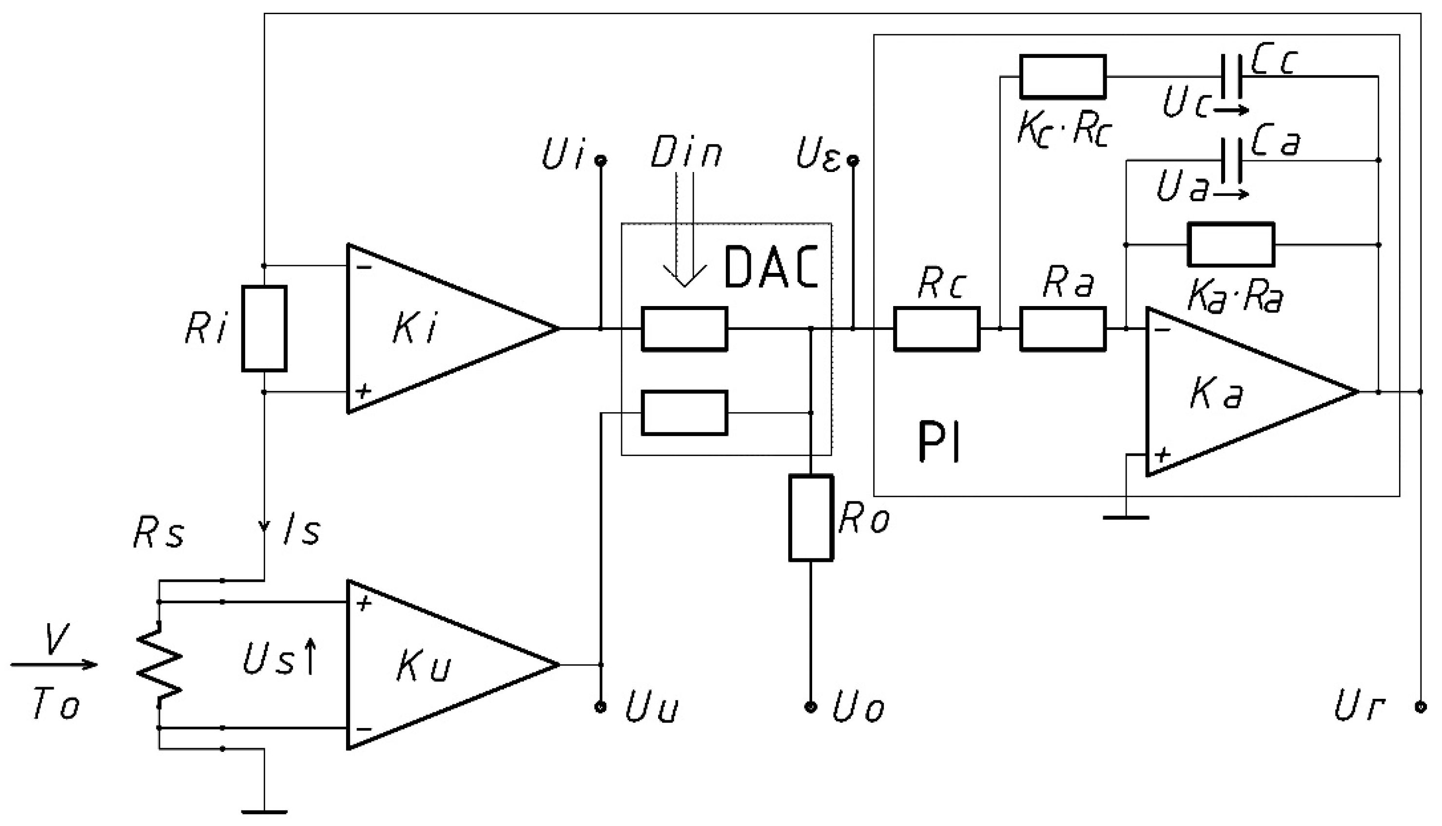
A laboratory constant-temperature anemometer that was developed and manufactured by the author was used in the research [18,19,20]. This anemometer enables the precise measurement of the sensor resistance and setting of the overheat ratio, as well as the adjustment and optimization of the dynamic parameters of the anemometer. The anemometer is built on the basis of the author’s concept of a non-bridge, controlled, constant-temperature system [18,19,20]. It is a digitally controlled, electronic, four-point supply system for the hot-wire sensor. The separation of the current and voltage leads of the sensor and digital setting of the resistance allow for precise anemometric measurements. The value of the sensor resistance is set by a digital signal fed to the multiplying digital-to-analog converter with the R-2R ladder. A simplified block diagram of the anemometer used in the research is presented in Figure 1.
The hot-wire Rs sensor is connected to the system by a four-wire line with separate current and voltage signals. The signal proportional to the sensor current from the Ri resistor is amplified in a Ki gain differential amplifier and fed to the input of the N-bit DAC. The converter functions as a system for comparing two analog signals, where the value of one of the signals is multiplied by a factor proportional to the digital control signal Din. A signal proportional to the sensor voltage Us, amplified in the Ku amplifier, is fed to the second input of the DAC. The converter is controlled by the digital signal Din. The output of the DAC converter is connected to the inverting input of the PI controller. Its task is to supply the sensor with a current that allows the error voltage Uε to be reduced to zero. In the steady state, the relationship is obtained:
According to Equation (2), the resistance of the hot-wire anemometric sensor, and therefore its temperature, is kept at a constant, set level. The system therefore performs a constant-temperature function. The resistance of the sensor is directly proportional to the value of the digital control signal Din, which allows the sensor overheat ratio to be determined. The dynamic properties of the electronic system are set by selecting the PI controller parameters. The output signals of the anemometer are as follows: Ui voltage proportional to the sensor current, from the Ki amplifier output, and Uu voltage proportional to the sensor voltage, from the Ku amplifier output.
In order to compare the results of the experimental studies of the anemometer frequency bandwidth with the results of a computer simulation, an anemometer model was developed and its parameters were determined. When constructing the model, the following assumptions were made:
- The sensor resistance is a linear function of its temperature;
- The sensor is described with a first-order dynamic model;
- Parasitic impedances are not taken into account;
- The operational amplifier describes the first-order inertial model taking into account the input resistance, gain and time constant;
- Differential amplifiers have high input resistance and are non-inertial;
- The digital-to-analog converter is non-inertial;
- In the system, there are no limitations to the range of signal variability;
- Non-linear effects related to saturation in electronic components are not taken into account.
The mathematical model of the system from Figure 1 was developed based on the equations describing its components. Three components determining the system model were distinguished: a hot-wire sensor, a resistance comparison system and a controller PI. The designations were adopted as presented in Figure 1. The hot-wire sensor description was based on the following equation [21]:
where
- Rs—Heated sensor resistance;
- Ro—Sensor resistance at flow temperature;
- Is—Sensor current;
- V—Flow velocity;
- IL, VL, τL, n—Model parameters;
- t—Time.
The used model parameters directly describe the basic metrological properties of the sensor and have an unambiguous dimension and simple physical interpretation. The IL parameter has the current dimension, and its value is the hypothetical sensor current at which, at zero velocity, the sensor overheat ratio
tends to infinity. At sensor current , at , the overheat ratio . The VL parameter has a velocity dimension; this dimension does not depend on the value of the exponent n. At velocity , in order to maintain the given overheat ratio, the sensor current is times greater than the current for . The dynamic properties of the sensor are described by the parameter τL. For zero flow velocity and a constant current of the sensor , the sensor resistance increases linearly, and over time, τL doubles its value.
The task of the four-point resistance comparation system is to compare the sensor resistance with a set value by a digital signal and to generate an error signal. This system is described by the equation showing the dependence of the error voltage Uε on the output voltage of the controller Ur that is supplying the resistance comparison system:
The voltage U0 is the anemometer offset voltage. This is a small additional voltage subtracted from the error voltage. It allows a test signal to be introduced into the circuit in accordance with Equation (1).
The anemometer uses an analog controller with a proportional–integral structure. The PI controller is built on a single operational amplifier, taking into account the real properties of the operational amplifier. For the real operational amplifier, a first-order inertial model with ideal operational amplifier was adopted, taking into account finite input resistance, limited gain and inertia. For the considered issues, this model is a good approximation of the real operational amplifier. The amplifier together with external R and C elements performs the function of a proportional–integral controller. By denoting the time constant of the inertial operational amplifier model,
and the integrator time constant,
the controller PI describes the system of equations:
The voltages Ur and Uc as well as the resistance of the sensor Rs were adopted as the state variables for the description of the constant-temperature anemometer system. Taking into account the equation describing the sensor (3), the equation of the resistance comparation system (5) and the equations of the PI controller (8), (9), we obtain a system of equations describing the anemometer model in the form:
The above equations, together with the initial conditions for the state variables, constitute a mathematical model of the constant-temperature anemometer system and allow for its model tests. The procedure for determining and validating the parameters of the measurement system model and the modeling methodology used by the author are described in [12,18,19,20,21]. The parameters of the sensors and the constant-temperature system used in the experimental tests were determined for model tests. They are summarized in Table 1 and Table 2.
For these parameters, the course of the anemometer frequency response was determined by the computer simulation method. The simulation consisted of examining the amplitude of the anemometer response to the sinusoidal forcing changes in the flow velocity at the set frequencies. The MATLAB environment was used for the simulation tests.
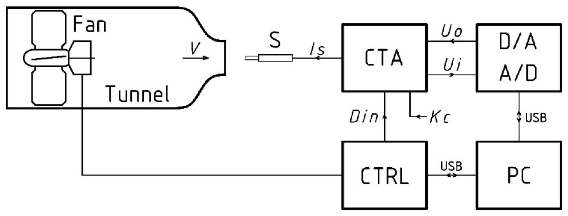
The block diagram of the experimental stand for testing the method of determining the shape of the frequency bandwidth of the constant-temperature anemometer is shown in Figure 2.
Two hot-wire sensors S with a resistance at ambient temperature of about 5 ohms were used for the tests. The sensors had tungsten filaments that were 3 and 5 microns in diameter. The overheat ratio of 1.8 was used in tests. The research into the CTA anemometer bandwidth was carried out for four values of air flow velocities V set in the wind tunnel: 1, 3, 10 and 30 m/s. The dynamic parameters of the anemometer were adjusted by means of a square test for the velocity value of 10 m/s. The gain and time constant of the controller PI of anemometer were adjusted to obtain a 15% overshoot in the anemometer response to a square excitation. Such regulation ensures the optimal frequency response for given operating conditions [4,5]. The Rohde & Schwarz RTM3K-24 digital signal generator D/A and analog signal recorder A/D were used to determine the frequency response of the anemometer CTA for each set velocity value. The parameters of the experiment were controlled from a PC via USB using the CTRL circuit.
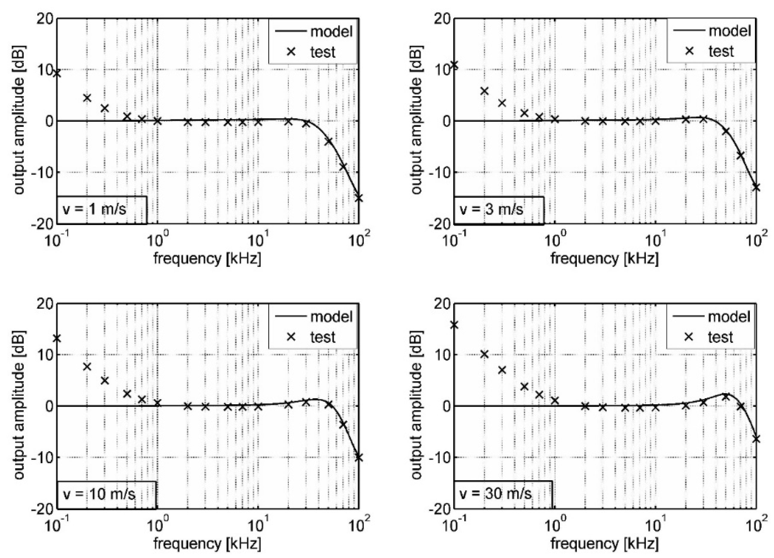
The test signal described by Equation (1) was generated for the frequencies of 0.1, 0.2, 0.3, 0.5, 0.7, 1, 2, 3, 5, 7, 10, 20, 30, 50, 70 and 100 kHz. The values of the U0 and U1 offset were assumed to be 10 mV. For each frequency, the amplitude of the output signal from the CTA anemometer was recorded according to the procedure described. Thus, for both sensors, the waveforms of the anemometer’s response to a sinusoidal voltage signal with an amplitude inversely proportional to the frequency were determined. The MATLAB mathematical modeling bandwidth shape results of the measurement system were used as reference graphs. In the MATLAB modeling process, the anemometer frequency response was determined for simulated sinusoidal changes in flow velocity. Figure 3 shows the obtained waveforms of the anemometer bandwidth for a sensor with a 3 micron filament.
The graphs presented in Figure 3 show that for frequencies above 1 kHz, the course of the anemometer frequency response determined by the described method practically coincides with the modeling results. In the range of low frequencies, we assume the course of the frequency response to be flat. As the velocity increases, the bandwidth widens, and the gain for high frequencies increases as well. The performed sinusoidal test also provides information on the dynamic properties of the sensor. In this case, the value of the characteristic frequency at which the sensor’s thermal inertia significantly limits changes of its temperature from about 700 Hz for a velocity of 1 m/s to 2 kHz for a velocity of 30 m/s.
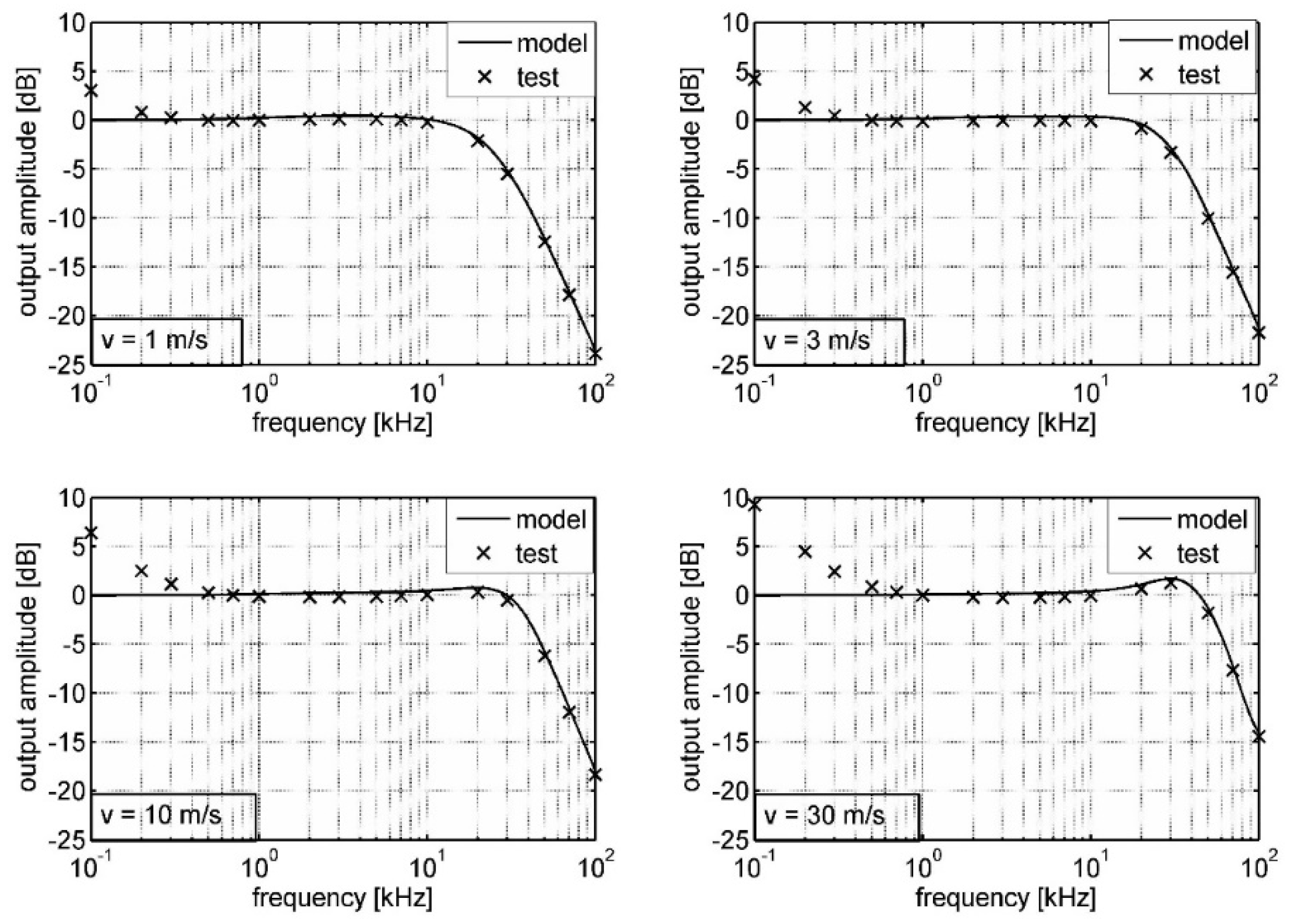
The corresponding graphs for the sensor with a tungsten filament with a diameter of 5 microns are shown in Figure 4.
In this case, we also obtain a similar course of the modeling results and the sinusoidal test, with the bandwidth limit frequency being correspondingly smaller due to the greater thermal inertia of the sensor. The characteristic frequencies at which the sensor’s thermal inertia significantly limits changes of its temperature is from about 300 Hz for a velocity of 1 m/s to 700 Hz for a velocity of 30 m/s. The determined limit frequencies at which there is a 3 dB decrease in the anemometer bandwidth for the modeling fm and the described sinusoidal test fs are summarized in Table 3.
The limit frequencies of the anemometer bandwidth, determined by both methods, have a similar value with an accuracy of 5%, while the sinusoidal test gives slightly lower values than the modeling. This may result from the 0 dB reference level adopted in this sine wave method. Both the modeling method and the presented sinusoidal test are burdened with metrological uncertainty, but the similar results allow the conclusion that the presented experimental test method allows for the determination of the bandwidth shape of a real measuring instrument with a good approximation.
4. Conclusions
The presented method allows us to experimentally determine the course of the constant-temperature anemometer bandwidth for given, set operating conditions. This method differs from the standard square and sine test, which only determines the cut-off frequency. Additionally, in the presented method, we obtain information about the dynamic properties of the sensor. In the measurements of fast-changing and turbulent flows, the knowledge of the shape of the anemometer frequency bandwidth is important information that is necessary, for example, to determine the spectral power density in the flow, the distribution of kinetic energy in turbulent transport and other parameters. In many research issues, such information allows us to learn and understand the occurring physical phenomena and to optimize processes [22,23,24,25,26]. Determining the shape of the anemometer bandwidth is particularly important in the case of complex measurement systems with extremely optimized frequency parameters. In such cases, the shape of the bandwidth is generally not flat but may have certain frequencies gains or dips. The described method is particularly suitable for testing such situations. As already mentioned, due to the basic difficulties in determining the anemometer bandwidth in the reference, standard flow of a given frequency and amplitude of velocity fluctuation, the development and improvement of indirect methods is an important metrological issue. Therefore, the proposed method may complement the methods used so far, and in some cases, its use will allow the quality of the measurement process to be improved. The obtained preliminary results of the pilot studies allow us to positively assess the quality of the proposed method and its application potential. In further research, the proposed method can be applied to other types of anemometers and measuring instruments, and further research can also consider more complex metrological cases, taking into account, for example, changes in flow parameters such as temperature, pressure and gas composition.
Funding
This research was funded by National Science Centre, Poland, grant number 2017/25/B/ST8/00212. The APC was funded by National Science Centre, Poland.
Institutional Review Board Statement
Not applicable.
Informed Consent Statement
Not applicable.
Data Availability Statement
Not applicable.
Acknowledgments
The study was performed in the context of the grant 2017/25/B/ST8/00212: “An innovative method of testing high-amplitude, rapidly changing pulses flows–modelling, optimization and experimental verification” financed by National Science Centre, Poland.
Conflicts of Interest
The authors declare no conflict of interest.
References
- Duraisamy, K.; Iaccarino, G.; Xiao, H. Turbulence Modeling in the Age of Data. Annu. Rev. Fluid Mech. 2019, 51, 357–377. [Google Scholar] [CrossRef] [Green Version]
- Lomas, C.G. Fundamentals of Hot Wire Anemometry; Cambridge University Press: Cambridge, UK, 1986. [Google Scholar]
- Grosjean, N.; Graftieaux, L.; Michard, M.; Hübner, W.; Tropea, C.; Volkert, J. Combining LDA and PIV for turbulence measurements in unsteady swirling flows. Meas. Sci. Technol. 1997, 8, 1512. [Google Scholar] [CrossRef]
- Bruun, H.H. Hot-wire Anemometry. Principles and Signal Analysis; University Press: Oxford, UK, 1995. [Google Scholar]
- Freymuth, P. Frequency response and electronic testing for constant-temperature hot-wire anemometers. J. Phys. E Sci. Instrum. 1977, 10, 705–710. [Google Scholar] [CrossRef]
- Saddoughi, S.G.; Veeravalli, S.V. Hot-wire anemometry behaviour at very high frequencies. Meas. Sci. Technol. 1996, 7, 1297–1300. [Google Scholar] [CrossRef]
- Skotniczny, P.; Ostrogórski, P. Three-dimensional air velocity distributions in the vicinity of a mine heading’s sidewall. Arch. Min. Sci. 2018, 63, 335–352. [Google Scholar]
- Dziurzyński, W.; Krach, A.; Pałka, T. Shearer control algorithm and identification of control parameters. Arch. Min. Sci. 2018, 63, 537–552. [Google Scholar]
- Dadgara, F.; Venvika, H.J.; Pfeifer, P. Application of hot-wire anemometry for experimental investigation of flow distribution in micro-packed bed reactors for synthesis gas conversion. Chem. Eng. Sci. 2018, 177, 110–121. [Google Scholar] [CrossRef]
- Rusli, I.H.; Aleksandrova, S.; Medina, H.; Benjamin, S.F. Using single-sensor hot-wire anemometry for velocity measurements in confined swirling flows. Measurement 2018, 129, 277–280. [Google Scholar] [CrossRef]
- Li, D.J. Dynamic response of constant temperature hot-wire system under various perturbations. Meas. Sci. Technol. 2006, 17, 2665–2675. [Google Scholar] [CrossRef]
- Ligęza, P. Optimization of Single-Sensor Two-State Hot-Wire Anemometer Transmission Bandwidth. Sensors 2008, 8, 6747–6760. [Google Scholar] [CrossRef] [Green Version]
- Kegerise, M.A.; Spina, E.F. A comparative study of constant-voltage and constant-temperature hot-wire anemometers: Part II–The dynamic response. Exp. Fluids 2000, 29, 165–177. [Google Scholar] [CrossRef]
- Fan, D.; Xiaoqi, C.; Wong, C.W.; Li, J.-D. Optimization and Determination of the Frequency Response of Constant-Temperature Hot-Wire Anemometers. AIAA J. 2017, 55, 2537–2543. [Google Scholar] [CrossRef]
- Hutchins, N.; Monty, J.P.; Hultmark, M.; Smits, A.J. A direct measure of the frequency response of hot-wire anemometers: Temporal resolution issues in wall-bounded turbulence. Exp. Fluids 2015, 56, 18. [Google Scholar] [CrossRef]
- Freymuth, P. On higher order dynamics of constant-temperature hot-wire anemometers. Meas. Sci. Technol. 1998, 9, 534–535. [Google Scholar] [CrossRef]
- Li, D.J. The effect of electronic components on the cut-off frequency of the hot-wire system. Meas. Sci. Technol. 2005, 16, 766–774. [Google Scholar] [CrossRef]
- Ligeza, P. Four-point non-bridge constant-temperature anemometer circuit. Exp. Fluids 2000, 29, 505–507. [Google Scholar] [CrossRef]
- Ligęza, P. Construction and experimental testing of the constant-bandwidth constant-temperature anemometer. Rev. Sci. Instrum. 2009, 79, 096105. [Google Scholar] [CrossRef] [PubMed]
- Ligęza, P. An investigation of a constant-bandwidth hot-wire anemometer. Flow Meas. Instrum. 2009, 20, 116–121. [Google Scholar] [CrossRef]
- Ligęza, P. On unique parameters and unified formal form of hot-wire anemometric sensor model. Rev. Sci. Instrum. 2005, 76, 126105. [Google Scholar] [CrossRef]
- Fan, Y.; Arwatz, G.; Buren, T.W.; Hoffman, D.E.; Hultmark, M. Nanoscale sensing devices for turbulence measurements. Exp. Fluids 2015, 56, 138. [Google Scholar] [CrossRef]
- Wang, J.J.; Hu, H.; Chen, C.Z. The Effect of Sensor Dimensions on the Performance of Flexible Hot Film Shear Stress Sensors. Micromachines 2019, 10, 305. [Google Scholar] [CrossRef] [PubMed] [Green Version]
- Ligęza, P.; Poleszczyk, E.; Skotniczny, P. Measurements of velocity profile in headings with the use of integrated hot-wire anemometric system. Arch. Min. Sci. 2008, 53, 87–96. [Google Scholar]
- Ligęza, P.; Poleszczyk, E.; Skotniczny, P. Method and the System of Spatial Measurement of Velocity Field of Air Flow in a Mining Heading. Arch. Min. Sci. 2009, 54, 419–440. [Google Scholar]
- Ligeza, P. Use of Natural Fluctuations of Flow Parameters for Measurement of Velocity Vector. IEEE Trans. Instrum. Meas. 2014, 63, 633–640. [Google Scholar] [CrossRef]
Figure 1.
Block diagram of the anemometer used in the research.

Figure 2.
Block diagram of the experimental stand.

Figure 3.
The frequency response of the constant-temperature anemometer for a sensor with a 3 micron filament for air velocities of 1, 3, 10 and 30 m/s determined by the MATLAB modeling (-) and experimental sinusoidal test (x) method.
Figure 3.
The frequency response of the constant-temperature anemometer for a sensor with a 3 micron filament for air velocities of 1, 3, 10 and 30 m/s determined by the MATLAB modeling (-) and experimental sinusoidal test (x) method.

Figure 4.
The frequency response of the constant-temperature anemometer for a sensor with a 5 micron filament for air velocities of 1, 3, 10 and 30 m/s determined by the MATLAB modeling (-) and experimental sinusoidal test (x) method.
Figure 4.
The frequency response of the constant-temperature anemometer for a sensor with a 5 micron filament for air velocities of 1, 3, 10 and 30 m/s determined by the MATLAB modeling (-) and experimental sinusoidal test (x) method.


Table 1.
Parameters of the sensors used in model and experimental tests.
| Probe Filament | T0 (K) | Ro (Ω) | η | IL (mA) | VL (m/s) | τL (ms) | n |
|---|---|---|---|---|---|---|---|
| Tungsten 3 μm | 293 | 5.11 | 1.8 | 41.7 | 7.19 | 0.42 | 0.5 |
| Tungsten 5 μm | 293 | 5.23 | 1.8 | 60.4 | 2.68 | 1.34 | 0.5 |
Table 2.
Parameters of the anemometer used in model and experimental tests.
| Ri (Ω) | Rc (Ω) | Ra (MΩ) | Ku | Ki | Ka | Kc3 | Kc5 | τa (ms) | τc (ms) |
|---|---|---|---|---|---|---|---|---|---|
| 10 | 100 | 1 | 10 | 10 | 106 | 29.1 | 40.5 | 10 | 0.15 |
Table 3.
Determined constant-temperature anemometer limit frequencies of the tested probes for modeling fm and sinusoidal test fs.
Table 3.
Determined constant-temperature anemometer limit frequencies of the tested probes for modeling fm and sinusoidal test fs.
| Probe | 3 μm | 5 μm | ||||||
|---|---|---|---|---|---|---|---|---|
| v (m/s) | 1 | 3 | 10 | 30 | 1 | 3 | 10 | 30 |
| fm (kHz) | 47.4 | 56.3 | 68.8 | 88.9 | 24.0 | 33.6 | 41.9 | 57.1 |
| fs (kHz) | 45.0 | 55.1 | 67.4 | 86.6 | 23.0 | 29.9 | 40.4 | 55.3 |
Publisher’s Note: MDPI stays neutral with regard to jurisdictional claims in published maps and institutional affiliations. |
© 2021 by the author. Licensee MDPI, Basel, Switzerland. This article is an open access article distributed under the terms and conditions of the Creative Commons Attribution (CC BY) license (https://creativecommons.org/licenses/by/4.0/).
Share and Cite
MDPI and ACS Style
Ligęza, P. Constant-Temperature Anemometer Bandwidth Shape Determination for Energy Spectrum Study of Turbulent Flows. Energies 2021, 14, 4495. https://0-doi-org.brum.beds.ac.uk/10.3390/en14154495
AMA Style
Ligęza P. Constant-Temperature Anemometer Bandwidth Shape Determination for Energy Spectrum Study of Turbulent Flows. Energies. 2021; 14(15):4495. https://0-doi-org.brum.beds.ac.uk/10.3390/en14154495
Chicago/Turabian StyleLigęza, Paweł. 2021. "Constant-Temperature Anemometer Bandwidth Shape Determination for Energy Spectrum Study of Turbulent Flows" Energies 14, no. 15: 4495. https://0-doi-org.brum.beds.ac.uk/10.3390/en14154495
Note that from the first issue of 2016, this journal uses article numbers instead of page numbers. See further details here.