Article

Heating and Lighting Load Disaggregation Using Frequency Components and Convolutional Bidirectional Long Short-Term Memory Method

1
School of Engineering, The University of Edinburgh, Edinburgh EH9 3DW, UK
2
School of Informatics, The University of Edinburgh, Edinburgh EH8 9AB, UK
3
Faculty of Electronic Engineering, University of Nis, 18000 Niš, Serbia
*
Author to whom correspondence should be addressed.
Submission received: 6 July 2021 / Revised: 26 July 2021 / Accepted: 5 August 2021 / Published: 8 August 2021
(This article belongs to the Special Issue Load Modelling of Power Systems)

Abstract

:
Load disaggregation for the identification of specific load types in the total demands (e.g., demand-manageable loads, such as heating or cooling loads) is becoming increasingly important for the operation of existing and future power supply systems. This paper introduces an approach in which periodical changes in the total demands (e.g., daily, weekly, and seasonal variations) are disaggregated into corresponding frequency components and correlated with the same frequency components in the meteorological variables (e.g., temperature and solar irradiance), allowing to select combinations of frequency components with the strongest correlations as the additional explanatory variables. The paper first presents a novel Fourier series regression method for obtaining target frequency components, which is illustrated on two household-level datasets and one substation-level dataset. These results show that correlations between selected disaggregated frequency components are stronger than the correlations between the original non-disaggregated data. Afterwards, convolutional neural network (CNN) and bidirectional long short-term memory (BiLSTM) methods are used to represent dependencies among multiple dimensions and to output the estimated disaggregated time series of specific types of loads, where Bayesian optimisation is applied to select hyperparameters of CNN-BiLSTM model. The CNN-BiLSTM and other deep learning models are reported to have excellent performance in many regression problems, but they are often applied as “black box” models without further exploration or analysis of the modelled processes. Therefore, the paper compares CNN-BiLSTM model in which correlated frequency components are used as the additional explanatory variables with a naïve CNN-BiLSTM model (without frequency components). The presented case studies, related to the identification of electrical heating load and lighting load from the total demands, show that the accuracy of disaggregation improves after specific frequency components of the total demand are correlated with the corresponding frequency components of temperature and solar irradiance, i.e., that frequency component-based CNN-BiLSTM model provides a more accurate load disaggregation. Obtained results are also compared/benchmarked against the two other commonly used models, confirming the benefits of the presented load disaggregation methodology.

1. Introduction

Due to the recent deployment of demand-side management and demand-responsive load control schemes, load disaggregation is becoming increasingly important for balancing renewable generation and provision of various system support services [1,2]. Two additional drivers for a significant increase of interest in load disaggregation are the much higher availability of demand datasets from advanced and intelligent monitors, e.g., smart meters, as well as the development of efficient neural/recurrent network and deep learning modelling methods. Load disaggregation denotes a general process in which specific load types or load categories are identified in the measured aggregated (i.e., total) electricity demands. Typically, load types and categories of interest for disaggregation are appliances, or groups of appliances that share similar electrical and/or consumption characteristics, e.g., demand-manageable loads, such as heating or cooling loads.
In cases where disaggregation is performed on total demands measured by a single electricity meter (i.e., for a single customer), the common term is “nonintrusive appliance/load monitoring” (NIALM/NILM), as opposed to the monitoring of individual appliances/loads by separate meters, which is denoted as “intrusive appliance/load monitoring” (IALM/ILM) [3,4]. Load disaggregation is readily available for ILM, as the loads of interest are directly monitored, while NILM-based load disaggregation faces several challenges. The main idea behind NILM is that different load types will have different energy consumption “signatures” or “patterns”, which will then allow for their identification in the total demand, assuming measured data are available with a sufficient resolution. However, the energy consumption signatures/patterns may vary strongly, depending on the appliance-specific characteristics, weather conditions, user settings, and habits, or wider socio-economic factors [5], making the identification of the distinctive load types difficult. A significantly more challenging problem is load disaggregation at a distribution network substation level, where available measurements are total demands of a large number of customers, whose individual smart meter data may not be accessible, e.g., due to data privacy/ownership concerns.
Direct load disaggregation approaches aim at detecting specific changes in total demand that can be allocated to the use of individual appliances, e.g., their on/off switching [6]. Various clustering and classification algorithms are widely applied to identify unique load signatures in demand time series, such as support vector machines [7], decision trees [8], and combinatorial optimisation (CO) [9]. If the sufficiently labelled datasets for both total demands and individual load type demands are available, as in ILM-based approaches, hidden Markov models (HMM) and their variants (e.g., factorial hidden Markov model, FHMM) can be used to explore patterns of individual appliances and their combinations [10,11]. Frequency-based analysis methods, including Fourier [12] and wavelet [13] transforms, are also used to capture on/off switching events, or to identify load types with specific harmonic emission signatures. Usually, these methods are inaccurate when there is high noise in the measured data, and their complexity and computational times significantly increase when the numbers of appliances and/or their operating states increase.
As mentioned, deep learning models are being increasingly used in many areas and in various applications, including load disaggregation [3,5,14,15], where improvement in accuracy and performance for identifying the underlying load profiles and demand patterns have been reported. However, these approaches are often criticised as “black box” methods, because they are difficult to interpret and as their results are sensitive to the settings of model hyperparameters [16]. Accordingly, the majority of the deep learning models in current literature are simply built and tuned using the available data, without performing further exploration or analysis of the modelled processes. For example, the accuracy of the built models will increase if domain expert knowledge is used to analyse and extract specific characteristics from available data. This is usually denoted as “feature engineering”, as the extracted features may be essential for understanding the modelled process, and as the selection of the most representative data properties may result in performance improvement. Ref. [17] presents a review of features for appliance classification in load disaggregation (low and high frequency, steady state, and transient categories), showing that systematic feature selection can improve accuracy. Ref. [18] considers and compares electrical and statistical features for load disaggregation, confirming the importance of selecting both appropriate features and algorithms.
This paper aims to contribute to the existing research in the general area of load disaggregation by proposing a novel frequency domain decomposition and correlation method, which requires only synchronised time series of active power demands and weather variables (temperature and solar irradiance). The methodology is illustrated on several case studies with actual measurement data, demonstrating that the use of correlated frequency components as the additional features in the state-of-the-art neural network load disaggregation model provides more accurate results than the same neural network model without frequency components. The three main contributions of the paper are (a) introduction of a new Fourier series regression method for decomposition of synchronised demand and weather time series into target frequency components, and (b) formulation of an approach for evaluating correlations between obtained frequency components, allowing to select components with strongest correlations as the additional explanatory variables for the load disaggregation, and (c) comparison of the performance of deep learning model in which correlated frequency components are used as the additional explanatory variables with a conventional “black box” deep learning model (without frequency components), showing that the frequency component-based model provides a more accurate load disaggregation.
After this introductory section, Section 2 presents a novel frequency component-based load disaggregation method, where specific combinations of single-component Fourier series decomposition of targeted periodical components of the total demand are correlated with the corresponding frequency components of weather variables (temperature and solar irradiance). These results are then used to indicate changes of heating and lighting loads, as these have strong negative correlations with temperature, and solar irradiance, respectively. Afterwards, Section 3 presents a CNN-BiLSTM load disaggregation model, for which the most appropriate hyperparameters are selected using Bayesian optimisation (BO) approach. The analysis in Section 2 and Section 3 is illustrated on different case studies, showing that the accuracy of the disaggregated load types improves if specific frequency components of the total demand, temperature and solar irradiance are used as the additional explanatory variables in the CNN-BiLSTM model. Section 3 also presents comparison and benchmarking of the proposed frequency component-based CNN-BiLSTM model with a naïve CNN-BiLSTM model (without frequency components) and two other commonly used models (CO and FHMM), confirming benefits of the presented load disaggregation methodology. Finally, Section 4 gives the main conclusions from the presented analysis. Figure 1 provides a “block diagram” illustration of the proposed load disaggregation approach, which also shows a layout of the overall analysis presented in the paper.

2. Selection of Target Frequency Components for Fourier Series Decomposition and Correlational Analysis

Periodical changes in weather conditions (e.g., daily and seasonal variations in temperature and solar irradiation) have a strong impact on the periodical changes in residential electricity demands, which are also influenced by socio-economic factors, e.g., weekly schedule of working days and weekend days [5]. For example, space heating appliances in a cold-climate location are mainly used in winter and spring/autumn seasons, when the ambient temperature is low, while demand for lighting is also usually higher in winter, because of the shorter duration of daylight hours. This results in a strong negative correlation of heating load demand with temperature and a similarly strong negative correlation of lighting load with solar irradiance. As the temperature and solar irradiance also exhibit periodical changes on both longer-term scale (e.g., seasonal and annual variations) and shorter-term scale (e.g., diurnal or daily variations), the actual variations in electricity demands for heating and lighting are generally expected to follow these periodical changes. Accordingly, the correlational analysis can be used to select the most strongly correlated frequency components, which then can indicate portions of the disaggregated demands that contain higher contributions from specific load types and therefore can serve as additional variables for a more accurate load disaggregation model.
This section first describes the available residential demand datasets. Afterwards, it presents a novel Fourier series regression (FSR) method with different window sizes, where each window allows to extract a specific single-frequency component from the total demand, temperature, and solar irradiance time series data, demonstrating that these frequency components can relatively accurately reconstruct the original dataset. Spearman correlation coefficients [19] are used to quantify correlations, in order to identify combinations of specific disaggregated frequency components that have stronger negative correlations than the original non-disaggregated data.

2.1. Description of Available Datasets

To illustrate the proposed methodology, this paper uses three available datasets, which are either measured or pre-processed to have a temporal resolution of 30 min. The first is Almanac of Minutely Power dataset (AMPds2) Version 2 from [20], which contains total active and reactive power demand measurements, as well as measurements of the active power of the heat pump of a single household located in Burnaby, Canada, from 1 April 2012 to 31 March 2014. The second dataset is UK Domestic Appliance-Level Electricity (UK-DALE) [21], consisting of measurements of total active and reactive power demands and measurements of the active power of lighting load for one household in London, UK, from 18 March 2013 to 17 March 2016. For both AMPds2 and UK-DALE datasets, the synchronous data for meteorological parameters (temperature and solar irradiance) in the same geographical location are obtained from an external data source, MERRA-2 [22]. Unlike the first two household-level datasets, the third dataset is related to a medium voltage (MV) substation-level measurements of predominantly residential total active and reactive power demands in a city in Scotland, UK, together with temperature and solar irradiance recordings from 1 January 2007 to 31 December 2012 [23]. In this case, the measurements of disaggregated loads, including heating and lighting loads, are not available. All three datasets are used as the case studies for Fourier series regression and correlation analysis, where in the next sections AMPds2 is used for the identification of heating load from the total demand using correlations with temperature, UK-DALE is analysed for the identification of lighting load in the total demand using correlations with solar irradiance, while MV level dataset is used for considering both the correlation between the total demand and temperature, and correlation between the total demand and solar irradiance.

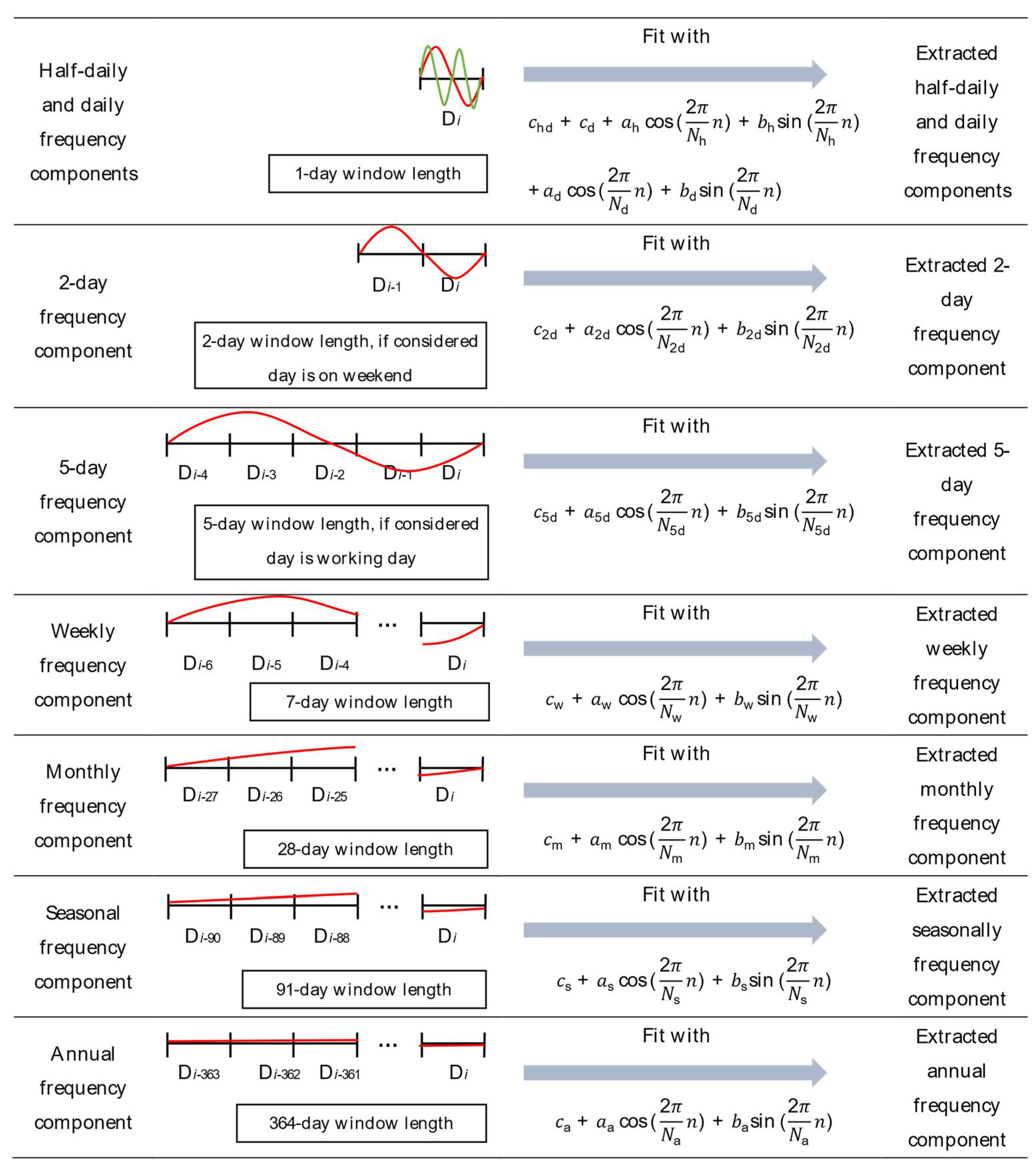
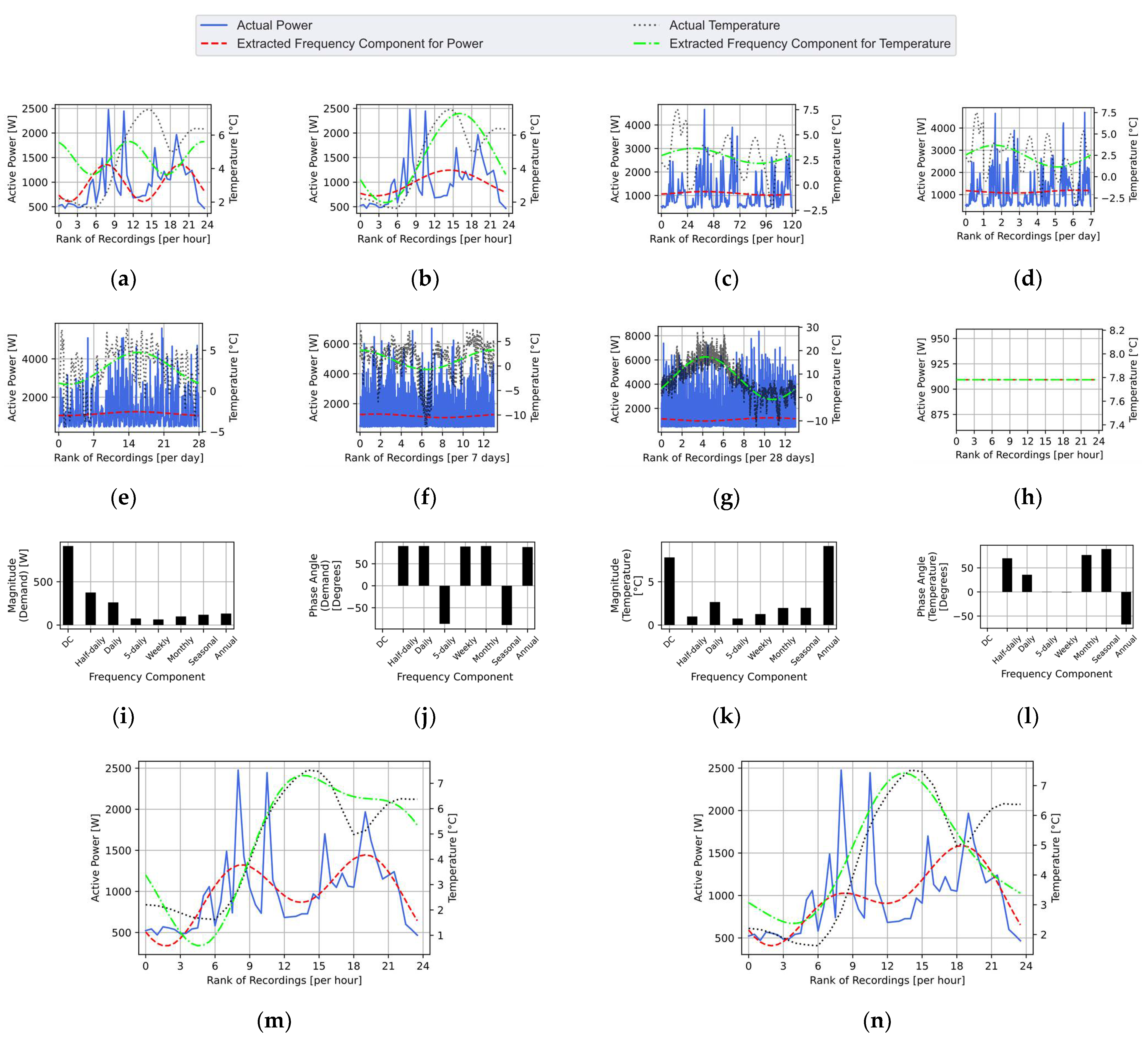
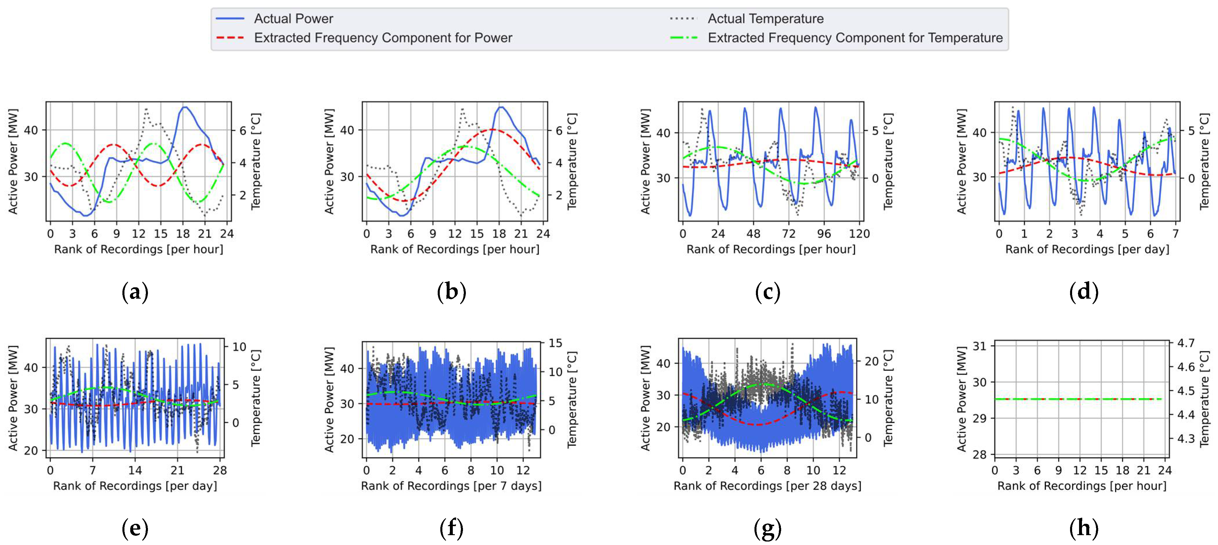
2.2. Disaggregation through Targeted Single-Components Fourier Series Decomposition

Fourier series decomposition is a commonly used approach for representing periodical function or “signal” with a sum of ideally sinusoidal components and one constant term, usually written as:
f ( n ) = a 0 2 + k = 1 a k cos ( 2 π k N n ) + k = 1 b k sin ( 2 π k N n )
where: f(n) is the input periodical function/signal with period N; ak and bk are Fourier coefficients calculated by integrals 2 N 0 N f ( n ) cos ( 2 π k N n ) d n and 2 N 0 N f ( n ) sin ( 2 π k N n ) d n , respectively; and a 0 2 = 1 N 0 N f ( n ) d x represents the non-periodical, i.e., constant DC component.
For extracting the single frequency components, as it is done in this paper for the target periodical components with specific window lengths, the following relation can be used:
f ( n ) = c x + a x cos ( 2 π N x n ) + b x sin ( 2 π N x n )
where: cx is the DC component if f(n) is fitted and determined by Fourier coefficients ax and bx, and the frequency is 1/Nx.
If Equation (2) is applied with the multiple window lengths, where each window represents one identified or dominant periodical component in the analysed time series, and where for each component related window length is applied in successive steps, the sum of the considered frequency components is effectively an alternative to the fitting by Equation (1). The advantage of Equation (2) is that it allows for extracting different frequency components in a computationally efficient way by simply applying different observation window sizes, where the length of each window defines the fundamental period of each extracted component. For example, if Equation (1) is applied on a time series length of one calendar year, it will provide annual, seasonal, monthly, weekly, and daily components, where an annual component is fundamental, and other mentioned components are harmonics. However, this approach will result in an equal daily component for all days, which is fitted based on the average of all days. On the other hand, Equation (2) can be applied separately for each day (window length of one day), then for the week to which that day belongs (window length of one week), then for the corresponding month (window length of one month), then corresponding season (window length of one season) and finally for the year to which that day belongs (window length of one year), providing considered frequency components for the day of interest. Afterwards, this procedure can be repeated for the next day, and so on. A comparison between Fourier series decomposition by Equation (1) and by applying selected components using Equation (2) is provided later in this section.
If the exact decomposition through the infinite Fourier series in Equation (1) is not of interest, successive application of Equation (2) allows to obtain selected or targeted frequency components, e.g., to disaggregate total demand in periodically changing daily, weekly and seasonal components. In a matrix notation, it can be written as:
y = X β   [ f ( 1 ) f ( 2 ) f ( N ) ] = [ 1 cos ( 2 π N x × 1 ) sin ( 2 π N x × 1 ) 1 cos ( 2 π N x × 2 ) sin ( 2 π N x × 2 ) 1 cos ( 2 π N x × N ) sin ( 2 π N x × N ) ] [ c x a x b x ]
which is equivalent to a regression problem. The value of β = [cx, ax, bx]T can be estimated using ordinary least squares (OLS), whose objective is to minimise the sum of squared residuals. The final results of OLS for β can be derived as (XTX)−1XTy. Refs [24,25] also apply regression techniques in period analysis, i.e., the least absolute shrinkage and selection operator (LASSO) as the regression regularisation. Also, the Goertzel algorithm [26], which is a type of discrete Fourier transform (DFT), may be used if only certain frequencies should be extracted, as in, e.g., real-time applications where short computational times are of high importance.
In terms of disaggregating measured total demand, temperature, and solar irradiance time series, only seven predefined frequency components are selected in this paper: half-daily, daily, two-daily (for two weekend days, if the considered day is on weekend), five-daily (for five working days, if the considered day is working day), weekly (for seven days of a week), monthly (for 28 days of a lunar month), seasonal (for 91 days of a season) and annual (for 364 days of a year, as 365 days will make most of the other frequency components to be interharmonics). The paper explicitly considers disaggregation of daily (24-h) demands, where the length of the output window is one day (see Section 3) and the corresponding daily time series is denoted as Di. The frequency components are obtained for the considered day of interest, including components with shorter and longer periodicity than one day. The half-daily component is calculated for the considered day as the 2nd harmonic of the Fourier series decomposition applied on the window length of one day (for which the daily component is the fundamental frequency component). The extension of the observation window allows for the identification of other (lower) frequency components. In that way, all considered frequency components for Di are extracted, so that the estimations on the considered day are based on the most relevant observations. This is illustrated in Figure 2.
It should be noted that there are several ways how observation windows could be extended: the one illustrated in Figure 2 is by going backwards in the historical data, as this is generally suitable for load forecasting applications, where the future realisations of the process are unknown and were using the future data to extend the observation window may cause a “look-ahead bias” [27]. For general analysis and characteristics or features extraction, as well as hindcasting applications, observation windows can be extended differently, e.g., by either putting the day of interest in the centre of the historical data, or at the beginning of the historical data.
Examples of the results of the frequency component disaggregation of the AMPds2 total demand and temperature data are shown in Figure 3. The first eight plots in Figure 3 (Figure 3a–h) show the selected frequency components, including DC, following the procedure illustrated in Figure 2. It can be seen that frequency components of total demand and temperature exhibit different correlations, both in terms of the full-length observation window, but also in terms of the increasing or decreasing trends/gradients on the considered day, which are discussed in more detail in Section 2.3. Figure 3i–l depict the magnitudes and phase angles of the considered frequency components of the total demand and temperature time series, while Figure 3m,n show the reconstructions of the non-disaggregated total demands and temperatures using only considered frequency components, i.e., by applying Equations (2) and (3) in Figure 3m, and by applying Equation (1) in Figure 3n.
Figure 3m combines and sums up only considered frequency components in Figure 3a–g, where DC component from Figure 3h is actually obtained by re-estimating DC component as a difference between the mean value of the original daily time series and the mean value of the summed frequency components. It can be seen in Figure 3m that the original non-disaggregated time series cannot be reconstructed with 100% accuracy, which is expected, as only a limited number of frequency components are used for the analysis. The considered frequency components can capture general increasing and decreasing changes during the considered day, therefore preserving important information in the approximation of the original time series. By comparing results for the considered day in Figure 3m,n, it can be seen that the Fourier series decomposition that extracts all frequency components by Equation (1) results in a less accurate reconstruction of the original time series than the proposed method. The biggest differences are in capturing morning peak in demand and unusual temperature increase during the evening time.
A numerical comparison between Figure 3m,n is presented in Table 1. Two widely used goodness-of-fit indices, mean absolute error (MAE) and root-mean-square error (RMSE), as well as the absolute and percentage errors between the actually measured demands and reconstructed demands in terms of the overestimated, underestimated and total energy (denoted as EO, EU, and ET, respectively) are used to evaluate the performance of the models [28,29]. In assessing the energy-based indices, it is assumed that the average half-hourly demand values are constant over the period of 30 min, so that the energy can be calculated as the power multiplied by the time. Only the timestamps when the reconstructed demand is higher/lower than the actual recordings are considered in the calculations of the amount of overestimated/underestimated energy and their percentages. Therefore, in some cases, there are higher percentages of overestimated/underestimated energy while their absolute values are lower, and vice versa, since different methods may have different time stamps for overestimated/underestimated energy. The results obtained by both conventional Fourier transform Equation (1) and the proposed FSR method provide accurate estimations for mean values, and their total errors are zero. However, the proposed FSR method has lower MAE, RMSE, and absolute overestimated and underestimated energy values.
Similarly, the results for the total demand and temperature recordings of the MV level datasets are shown in Figure 4, while Table 2 shows the comparisons between the proposed method and the conventional Fourier transform.
The same Fourier series regression method is applied to analyse the total load and solar irradiance time series, as shown in examples in Figure 5 and Figure 6, with Table 3 and Table 4 listing the comparison between the FSR method and the conventional Fourier transform. The presented results suggest that the proposed FSR method can reconstruct the original demand more accurately than the conventional Fourier transform, while also providing more informative results for the considered frequency components of interest.

2.3. Extraction of the Strongly Correlated Components

From the previous frequency component disaggregation results, it is clear that for a particular day, Di, the correlations between the total demand and temperature/solar irradiance are different for different frequency components. As the non-disaggregated total demand consists of the contributions of different types of the load, including heating load and lighting load and assuming that the heating load and lighting load are strongly negatively correlated with the temperature and solar irradiance, respectively, then disaggregated frequency components of the total demand with such strong negative correlations should contain a significant part of heating and lighting load. In other words, frequency components with strong negative correlations should help in the identification of heating and lighting loads. Accordingly, the further text is related to the analysis of these correlations.
The two most common metrics for correlational analysis are Pearson and Spearman correlation coefficients. As Pearson coefficient is a measure of linear correlation, this paper uses the Spearman coefficient, ρ, which can capture non-linear dependencies [30] to calculate and compare the correlations between total demand and temperature/solar irradiance:
ρ = cov ( r x ,   r y ) σ r x σ r y
where: rx and ry are the ranks of the two analysed data/time series, respectively; cov(∙) means covariance and σ represents the standard deviation. For the example results shown in Figure 3, Figure 4, Figure 5 and Figure 6, the Spearman correlation coefficients between the measured demand and temperature/solar irradiance time series on the considered days are calculated as 0.2323, −0.0579, 0.1791, and 0.1168, respectively. Note that the longer-term frequency components (with lower than daily frequencies) are obtained by extended observation windows, but only the considered/first days of longer windows are used in the calculations. The results for the correlational analysis of considered frequency components for the same days in Figure 3, Figure 4, Figure 5 and Figure 6 are presented in Table 5, where bold values indicate stronger negative correlations. Since the original time series and the FSR results may be quite different on various days/datasets, and one identified more negatively correlated frequency component may be different or may even increase the positive correlation on the other days, it is important to analyse every individual day and dataset separately.
Summing up frequency components with stronger negative correlations (the DC components are the same, as if using all frequency components) on the considered day will result in a new time series, whose characteristics, e.g., increasing or decreasing trends, can imply the changes in heating and lighting loads, with example results shown in Figure 7 and Figure 8. Although the reconstructed daily load profiles are not as accurate as if all considered frequency components are used (e.g., these with positive correlations), the Spearman correlation coefficients between the time series reconstructions using the combination of the selected frequency components with negative correlations are now −0.2210, −0.9679, −0.4798 and −0.4568 in Figure 7a,b, Figure 8a,b, respectively, i.e., all feature stronger negative correlations compared to the results using original/measured daily time series (i.e., 0.2323, −0.0579, 0.1791 and 0.1168). As the starting assumption/hypothesis is that the combination of the selected demand frequency components with stronger negative correlations with temperature and solar irradiance will contain significant portions of the heating and lighting loads, respectively, the new time series of these negatively correlated frequency components are used as additional information for the heating and lighting load disaggregation models presented in the next section.

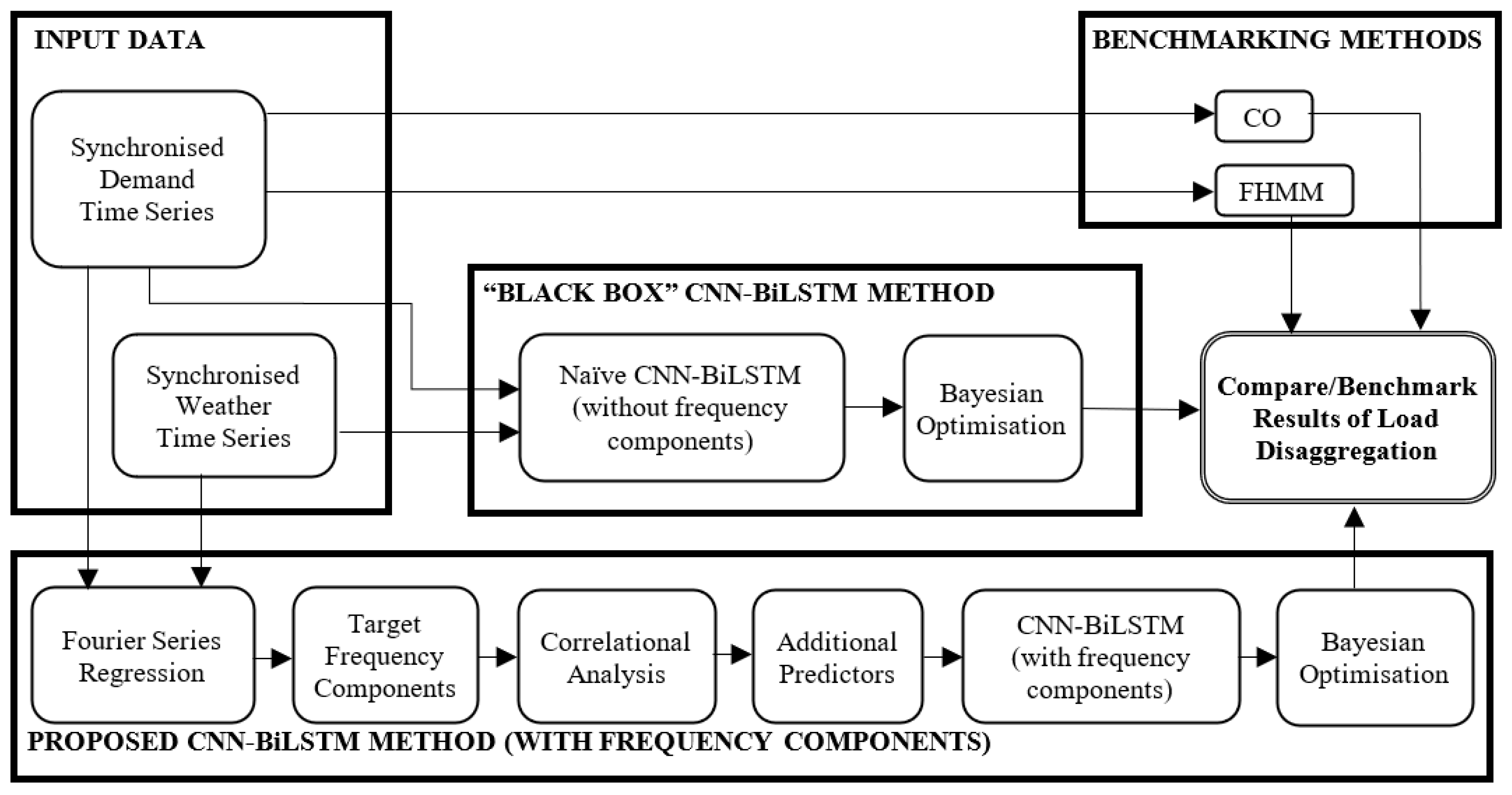
3. Neural Network Load Disaggregation Model

This section presents the load disaggregation model used in this paper, which is a neural network (NN) model, combining two widely used NN approaches: (1) recurrent neural network (RNN); and (2) convolutional neural network (CNN). However, before entering the time series predictor variables into the model, the frequency domain information is firstly extracted and analysed, following the Fourier series regression method in Section 2. The NN model utilises the embedded patterns from both the time domain and frequency domain, and it provides the final estimations for the disaggregated load. In addition, since hyperparameters of the NN model usually have a strong impact on the performance, but their optimal values are not known a priori, Bayesian optimisation is used to guide the tuning of the model hyperparameters.
In available datasets, AMPds2 has actual measurements for total load and heating load, while UK-DALE has measurements for total load and lighting load. Therefore, these two datasets are used to test the load disaggregation NN model. Each dataset is divided into training, validation, and test sub-sets. More specifically, in AMPds2, the measurements between 23 February 2014 and 31 March 2014 are used as test sub-set, and in UK-DALE, the recordings between 5 January 2016 and 17 March 2016 are used as test sub-set. For both datasets, the rest of the available data are used as the training and validation sub-sets, in the ratio of 90% to 10%.
The inputs of the NN models are (1) daily time series of the total active and reactive power demands; (2) synchronous daily time series of temperature and solar irradiance; (3) corresponding time and calendar variables, including month, day of the week, holiday indicator (Boolean variable) and daylight-saving time indicator (Boolean variable); and (4) synchronous daily time series of combinations of more negatively correlated frequency components of demand, temperature, and solar irradiance. All individual input features are treated as column vectors, i.e., columns that form the input data matrix. Adding of any additional predictor variable (e.g., synchronous combinations of more negatively correlated frequency components) is simply performed by appending a new column to the existing input matrix. The outputs of the load disaggregation models are heating load profile and lighting load profile on the considered day, which is the same day as the inputs for AMPds2 and UK-DALE, respectively. All continuous features are linearly scaled to a range between 0 and 1, and all categorical features are transformed using one-hot encoder [23].

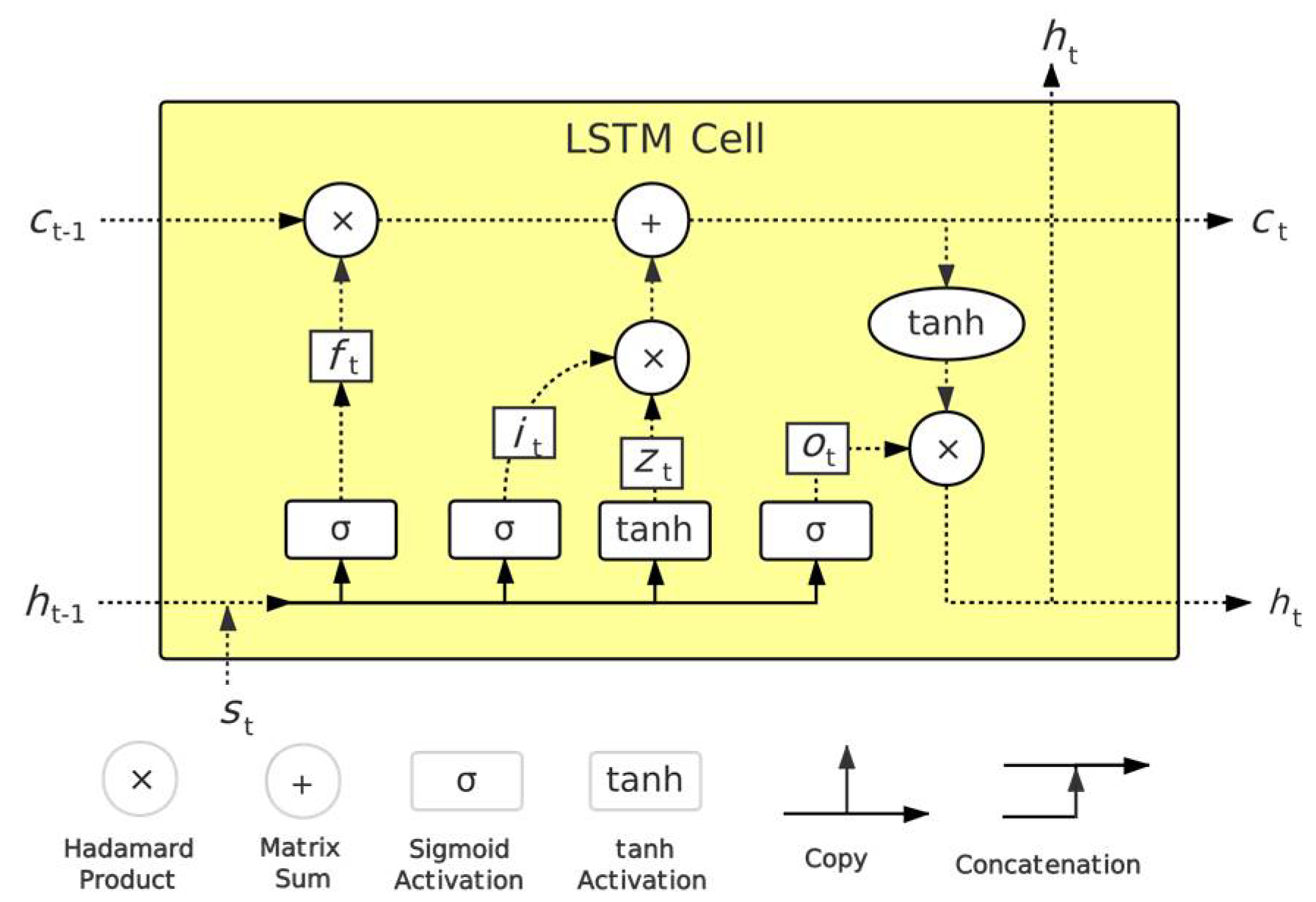
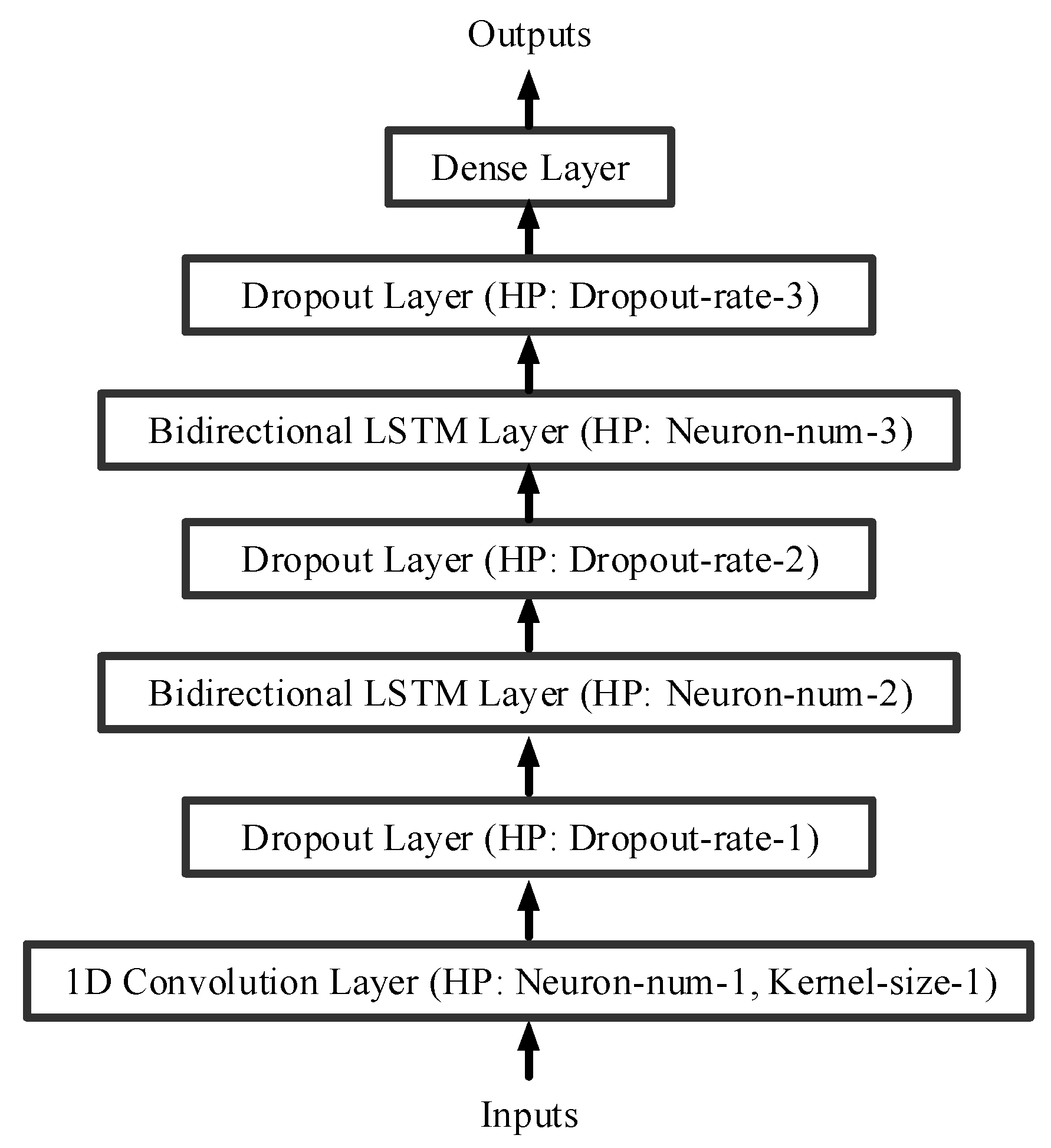
3.1. CNN-BiLSTM Load Disaggregation Model

A convolutional neural network is a type of deep learning model commonly used in image processing and computer vision applications. Compared to a more general NN model architecture, e.g., a multilayer perceptron (MLP), CNN is less prone to overfitting issues, as it does not use simple full-connections, but it embeds the complex data patterns into the smaller and simpler filters through the convolution [31]. The convolution operation is performed by a convolution matrix, i.e., kernel, which dot-multiplies the target matrix from which the features are extracted as:
f m ( i , j ) = k m t m ( i , j ) = Δ i = Δ i min Δ i max Δ j = Δ j min Δ j max k m ( Δ i , Δ j ) g m ( i + Δ i , j + Δ j )
where: gm is the target matrix, km is the kernel matrix, and fm is the filtered matrix after convolution; i and j are the row and column indices of the matrix, and Δi and Δj indicate the shifting along the row and column of the matrix, respectively. In terms of time series, the convolution operation is performed along the temporal dimension (a single dimension), which is effectively a 1D convolution, and ReLu (rectified linear unit) is used as the activation function [32].
In regression problems, RNN models, which are a type of deep learning models specialised for data sequences, are widely researched, and reported to achieve satisfactory accuracy. Unlike the MLP, the RNN is designed to have an internal state, where both the previous internal state and the current predictors are inputted into the RNN cell to produce the current output. The recursively updated internal state makes the RNN capable of memorisation.
When handling the long time series, however, naïve RNN methods tend to have other issues, such as “gradient vanishing” and “gradient exploding” in the backpropagation [33]. To overcome these problems, a long short-term memory (LSTM) method is developed, as it is relatively insensitive to gap lengths between the important sequence events in time series data [34]. Accordingly, every cell in the LSTM has three gates to control whether to remember, or to forget certain information, and whether to output it in each recursion. These three gates are trained, so that LSTM could remember important information and forget the irrelevant one, even in case of a long sequence. A general architecture of the LSTM cell is illustrated in Figure 9.
In Figure 9, st is the current input, and ht is the current output of the LSTM cell. State c (ct) is the cell state that changes extremely slow, and in most cases, it is very similar to the previous cell state (ct−1). State h (ht) stands for the hidden state, which varies a lot in the recursion and usually depends on both the current input and previous hidden state (ht−1). The computation can be summarised as:
f t = σ ( W f [ h t 1 , s t ] + b f )
{ i t = σ ( W i [ h t 1 , s t ] + b i ) z t = tanh ( W z [ h t 1 , s t ] + b z ) c t = f t × c t 1 + i t × z t
{ o t = σ ( W o [ h t 1 , s t ] + b o ) h t = o t × tanh ( c t )
where: Wf, Wi, Wz, Wo are weights parameters and bf, bi, bz, and bo are bias parameters of the LSTM cell; ft is the forget gate with ht−1 and st as inputs and it is activated by a sigmoid activation function σ; the remember gate signal i is also activated by a sigmoid activation function and another candidate vector z is activated by tanh function; the output gate signal ot again has a sigmoid activation and uses ht−1 and st the inputs. A more detailed discussion of LSTM cells can be found in [34]. The original LSTM architecture has only one direction and a bidirectional structure is firstly introduced in [35], to allow the signal to travel in both forward and backward directions. This is denoted as a bidirectional LSTM (BiLSTM) method, which could further reduce the errors.
As previously mentioned, deep learning and BiLSTM models are increasingly used for load disaggregation, as they can process long time series of data with complex patterns and identify target load profiles. As these models are often approached as “black box” modelling methods, the CNN-BiLSTM model proposed in this paper uses FSR-based frequency component decomposition as the additional explanatory variable/feature, in order to provide more accurate load disaggregation.
In the proposed CNN-BiLSTM load disaggregation model, the features in the predictors are firstly extracted with the CNN architecture, and outputs are padded with zeros evenly to the left and right, so that they have the same width dimension as the inputs before they enter into the two stacked layers of BiLSTM. As discussed, the convolution operation could reduce the variation in the input feature, which will then increase the temporal learning accuracy of the BiLSTM model [36]. Every layer is followed by a dropout layer to increase the generalisation ability and reduce overfitting, which refers to the random dropping-out of hidden and visible neurons in a certain layer [37]. The architecture of the CNN-BiLSTM is depicted in Figure 10, which also shows the hyperparameters (HPs) within the topology, which will be disused/optimised further in Section 3.2.

3.2. Tuning of Model Hyperparameter: Bayesian Optimisation (BO)

The optimal values of the NN model parameters are usually unknown and may change in different cases, even with only a small difference in the available training set. Furthermore, the final results may also be sensitive to the selected hyperparameters. As the hyperparameters cannot be optimised through the training process, an optimisation algorithm should be implemented. In this paper, Adam optimiser [38]) is used to find the best model (hyper)parameters (i.e., weight and bias values for every neuron) minimising the error function, since they are fixed once the NN model is instantiated. There are many types of hyperparameters in the proposed CNN-BiLSTM model, including the number of neurons (neuron_num) for trainable layers (CNN and BiLSTM), size of the kernel in CNN (kernel_size), and dropout rates for the dropout layer (dropout_rate), which represents the probability of dropout for the neurons in the previous layer. In addition, the learning rate for Adam optimiser (Adam learning rate) is also one of the model hyperparameters.
Random search or brute force looping for the combinations of different hyperparameter values can find the most appropriate hyperparameters in theory, but it requires significant computational times, since it does not use the information of previous trials and due to the “curse of dimensionality”. Instead, Bayesian optimisation (BO) is used, which is a heuristic searching method that uses the Gaussian process (GP) as a surrogate model and provides an exploitation-exploration trade-off through an acquisition function [39].
For the NN model hyperparameters denoted as x, and for the task of searching the best x for the NN model denoted as f(x), where f(∙) is an objective/cost black box function, its evaluation requires actual training and validation of the NN model, and the optimisation is to find x = argmaxx(f(x)). From the view of Bayesian optimisation, f(∙) can be described as a Gaussian process, i.e., a distribution over functions y = f(x)~GP, appreciating the uncertainty, which can be formulated as:
P ( y t + 1 | D 1 : t , x t + 1 ) = N ( μ t ( x t + 1 ) , σ t 2 ( x t + 1 ) )
μ t ( x t + 1 ) = k T K 1 y 1 : t
σ t 2 ( x t + 1 ) = k ( x t + 1 , x t + 1 ) k T K 1 k
K = [ k ( x 1 , x 1 ) k ( x 1 , x 2 ) k ( x 1 , x t ) k ( x 2 , x 1 ) k ( x 2 , x 2 ) k ( x 2 , x t ) k ( x t , x 1 ) k ( x t , x 2 ) k ( x t , x t ) ]
k = [ k ( x t + 1 , x 1 ) k ( x t + 1 , x 2 ) k ( x t + 1 , x t ) ] T
where: P(yt+1|D1:t, xt+1) is the posterior GP given observations D1:t = ((x1, y1), (x2, y2), …, (xt, yt)) and xt+1. Μt(∙) and σt(∙) are the mean and variance functions, respectively; k(∙) is the kernel function modelling the dependence among GP random variables, and K is the kernel matrix (i.e., covariance matrix), which should be positive definite. The choice of the kernel is not a trivial problem, as it determines almost all generalisation properties of a GP. Commonly used kernel functions include squared exponential kernel, rational quadratic kernel, and matern kernel (used in this paper), while further discussions and comparisons can be found in [39]. The next trial of hyperparameters, xt+1, is desired to lead to yt+1 = f(xt+1) to have both higher mean (exploitation) value and higher variance (exploration). Since they may not be simultaneously improved, a balance is needed and an additional criterion considering both μt and σt (known as acquisition function) is required. This paper selects confidence bounds, UCB(μt, σt), criterion proposed in [40] to determine the next trial of hyperparameters. In summary, Bayesian optimisation can be described iteratively for t + 1 trials as:
  • Fit the GP using D1:t = ((x1, y1), (x2, y2), …, (xt, yt));
  • Determine xt+1 = argmaxxt+1 (UCB(μt(xt+1), σt(xt+1)));
  • Evaluate yt+1 = f(xt+1);
  • Insert (xt+1, yt+1) into D1:t and obtain D1:t+1.
The BO method is applied to four instances of load disaggregation models separately and run 32 times each, which are: (1) AMPds2, heating load disaggregation, without FSR and correlation analysis results (AMPds2, w/o FR); (2) same as (1), but with FSR and correlation analysis results (AMPds2, w/FR); 3) UK-DALE, lighting load disaggregation, without FSR and correlation analysis results (UK-DALE, w/o FR); (4) same as (3), but with FSR and correlation analysis results (UK-DALE, w/FR). In every trial, the BO is executed three times and an average of error metrics is used, which can reduce the uncertainty and variance due to training and obtain a more reliable assessment of the considered settings of hyperparameters (thus, there are a total of 32 × 3 = 96 times of BO executions for each model instance). Each BO execution requires a maximum of 25,000 epochs on the training set, with minimised mean-square error (MSE) as the objective function. It assesses model performance with current hyperparameter settings on the validation set, which guides the searching direction of BO, so that the next groups of hyperparameters could potentially lead to a model with higher accuracy.
The set constraints of hyperparameters and the results of optimisation of hyperparameters by BO for all model instances are listed in Table 6. The constraints format [start:step:stop] means all values between start (inclusive) and stop (inclusive) with a distance of step, and the format [ele1, ele2, ele3] represent predefined set of possible values. It can be seen that in most cases, obtained optimised hyperparameters are different for different model instances. In particular, there are notable differences in the numbers of neurons for the 1D convolution layer. Even though the neuron numbers for two BiLSTM layers are quite different for two AMPds2 heating load disaggregation models, the dropout rates of the followed dropout layers are closer to each other, and similar analysis also applies to UK-DALE lighting load disaggregation models. For all four model instances, the identified most proper kernel size in the 1D convolution layer and the learning rate for Adam optimiser are the same, which are 5 and 0.0005, respectively. The load disaggregation results based on the models with the optimised hyperparameters are shown and compared in Section 3.3.

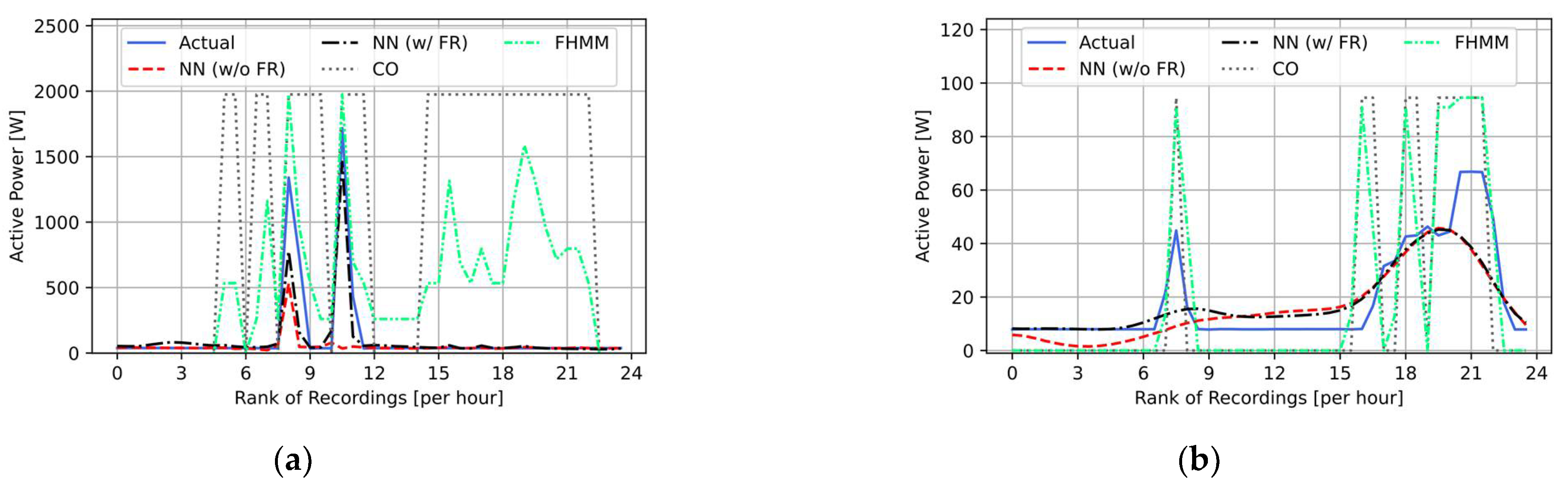
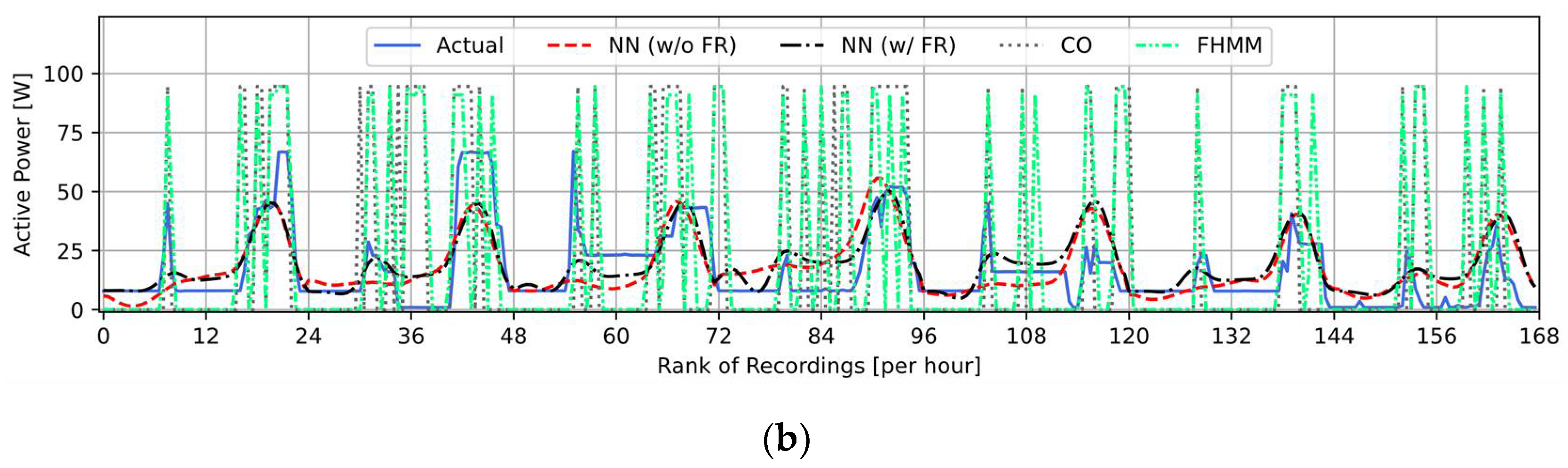
3.3. Load Disaggregation Results and the Benefits of Using Fourier Series Regression

As in previous comparisons of errors of time series reconstruction using conventional Fourier transform and proposed Fourier series regression (see Table 1, Table 2, Table 3 and Table 4), the same error metrics are used to assess the load disaggregation models. The example results of load disaggregation for AMPds2 and UK-DALE are shown in Figure 11, which are for the same days as in Figure 3 and Figure 6a (Monday, 24 March 2014) and Figure 5 and Figure 8a (Monday, 11 January 2016), respectively. Figure 12 shows the results for the two corresponding weeks. Table 7 and Table 8 show calculated error indices for these days/weeks, while Table 9 shows the overall model performance on the whole test set. In all comparisons, the results obtained by the proposed frequency component-based CNN-BiLSTM model (denoted as “NN w/FR”) are compared with a naïve CNN-BiLSTM model (without frequency components, denoted as “NN w/o FR”) and additionally benchmarked against two other commonly used NILM models from [41]: combinatorial optimisation (CO) and factorial hidden Markov model (FHMM) algorithms (more detailed discussions about CO ad FHMM can be found in [41]).
From examples in Figure 11, it is clear that the use of frequency components from the FSR-stage as additional predictors in the load disaggregation model can increase the accuracy of the estimations for both heating and lighting loads. Specifically, in the example of AMPds2, the identified more negatively correlated frequency components of demand capture peak during the morning time (Figure 7a), and this pattern helps the CNN-BiLSTM model to assign more attention and weight to this period, thus leading to a more precise capture of the heating load in this period (Figure 11a). Similar comparisons can be made between Figure 8a and Figure 11b for the lighting load disaggregation from the UK-DALE dataset, wherein this case lighting load has been more accurately estimated in the model with FSR results. In Figure 12, the weekly results for the CNN-BiLSTM model with correlated frequency components are consistently better than the results without them.
The calculated error indices in Table 7, Table 8 and Table 9 also demonstrate the benefits of using correlated frequency components, as these results have lower MAE and RMSE values for the example days, weeks, and in the whole test sets. In terms of the energy-based errors, although the overestimated and underestimated energy consumptions may not be simultaneously improved, the total energy estimations are generally better. There are some exceptions, e.g., in the week and whole test set comparisons for UK-DALE, where ET is seemingly worse if correlated frequency components are used, than if they are not used. This is because the EO and EU values increase or decrease by different levels, so the relative difference between them may be larger; in the weekly and whole test sets, the absolute (and percentage) EO and EU values are typically lower than in the cases when the correlated frequency components are not used.
The errors of the two NN models (frequency component-based CNN-BiLSTM model and naïve CNN-BiLSTM model) are all much smaller than the errors of CO and FHMM, used for benchmarking. The CO and FHMM seemingly correctly capture the phases of both morning and evening peaks, but the overall accuracy is not satisfactory. One reason is that both algorithms only consider the correlations between the total demand and individual appliances. Additionally, the performance of the CO model is impacted by treatment of each timestamp independently. However, both the CO and FHMM may perform better in the case of multiple appliance disaggregation, as they can analyse the combined demand of individual appliances. The CO usually contains a set of individual appliance models and aims to minimise the difference between the sum of estimations of all appliance demands and observed aggregated total demand. In FHMM, the separate appliances are also jointly considered, where each disaggregated load is modelled through one HMM and a hidden component of the HMM is the state of the individual appliance. In that way, all HMMs are combined to form one FHMM (or an equivalent HMM) in the final model to estimate the demand of all appliances.
All models are implemented using Python 3.8.5 and NumPy 1.8.5. The FSR-based decomposition and correlational analysis are built on Scikit-learn 0.23.2 and SciPy 1.5.4. The Bayesian optimisations and final CNN-BiLSTM models are implemented with KerasTuner 1.0.2 and TensorFlow 2.4.1, respectively. The CO and FHMM models are obtained from NILMTK 0.4.0. All calculations are done on a desktop running Microsoft Windows 10 21H1 operating system, with AMD Ryzen 1800X CPU, Nvidia GTX 1080ti GPU, and 32GB DDR4 RAM. The training times of all models are summarised and compared in Table 10. The computational time for BO is very long, since there are 96 times of BO executions in each case. The required times for BO and CNN-BiLSTM are given within square brackets, where the first number is related to the case where the FSR results are not used as an additional predictor, while the second number indicates the case where the model was run with the FSR results. It can be seen that considering the frequency domain information can also reduce the computation time in most cases.

4. Conclusions

This paper introduces a novel Fourier series regression method to extract selected frequency components (half-daily, daily, 2-daily, 5-daily, weekly, monthly, seasonal, and annual) from periodically changing non-disaggregated time series of active power demands, temperature, and solar irradiance. The presented method is illustrated on the three study cases with actually measured demands, corresponding to two household-level and one network substation-level datasets. The reconstructions by selected frequency components show that the original time series can be reasonably accurately represented, i.e., that the selected frequency components preserve the information on the total demand.
Afterwards, the paper presents the analysis of the correlations between different frequency components and demonstrates that specific individual frequency components of demands, temperature, and solar irradiance have stronger negative correlations than the original non-disaggregated time series. As the heating and lighting loads are expected to exhibit strong negative correlations with temperature and solar irradiance, the stronger negatively correlated frequency components are combined and used as the additional explanatory variables, i.e., as an additional feature of the CNN-BiLSTM load disaggregation model. The obtained results and comparisons demonstrate that the CNN-BiLSTM model in which correlated frequency components are used as the additional explanatory variables is more accurate for load disaggregation than the conventional/naïve CNN-BiLSTM model without frequency components (“black box model”).
The presented CNN-BiLSTM model adopts Bayesian optimisation to select the most appropriate hyperparameters for the four separate load disaggregation models, showing that the heating and lighting load are identified with higher accuracy when the correlated frequency components are used as the additional information during the disaggregation. The presented frequency component-based CNN-BiLSTM model is additionally benchmarked against two other-widely used NILM models (CO and FHMM), which both achieve lower accuracy of the load disaggregation than the presented model.
The methodologies and results presented in this paper are related to an initial investigation of the benefits of using correlated frequency components for load disaggregation. Further possible applications include, among the others, implementation in load forecasting studies and identification of the individual contributions from the load and distributed generation to the resulting/combined power flows when they are not separately metered. These are subjects of the current work by the authors.

Author Contributions

Conceptualization, methodology, validation, analysis, writing and editing, M.Z., S.Z., J.G., L.M.K. and S.Z.D.; software and visualization, M.Z. All authors have read and agreed to the published version of the manuscript.

Funding

This research was funded by an internal grant from School of Engineering, the University of Edinburgh, grant name: School of Engineering Ph.D. Scholarship.

Institutional Review Board Statement

Not applicable.

Informed Consent Statement

Not applicable.

Data Availability Statement

There are four data sets used in this article. (1) Ampds2 dataset [20] can be downloaded from https://dataverse.harvard.edu/dataset.xhtml?persistentId=doi:10.7910/DVN/FIE0S4 (accessed on 5 August 2021), (2) UK-DALE dataset [21] is publicly accessible from https://jack-kelly.com/data/ (accessed on 5 August 2021), (3) MERRA-2 dataset [22] can be found from https://gmao.gsfc.nasa.gov/reanalysis/MERRA-2/ (accessed on 5 August 2021), (4) MV level dataset is from industry partner and it is not a public dataset.

Conflicts of Interest

The authors declare no conflict of interest.

References

  1. Papaefthymiou, G.; Hasche, B.; Nabe, C. Potential of Heat Pumps for Demand Side Management and Wind Power Integration in the German Electricity Market. IEEE Trans. Sustain. Energy 2012, 3, 636–642. [Google Scholar] [CrossRef]
  2. Yao, E.; Samadi, P.; Wong, V.W.S.; Schober, R. Residential Demand Side Management Under High Penetration of Rooftop Photovoltaic Units. IEEE Trans. Smart Grid 2016, 7, 1597–1608. [Google Scholar] [CrossRef]
  3. Quek, Y.T.; Woo, W.L.; Logenthiran, T. Load Disaggregation Using One-Directional Convolutional Stacked Long Short-Term Memory Recurrent Neural Network. IEEE Syst. J. 2020, 14, 1395–1404. [Google Scholar] [CrossRef]
  4. Kelly, J.D. Disaggregation of Domestic Smart Meter Energy Data. Ph.D. Thesis, University of London, London, UK, 2017. [Google Scholar]
  5. Kaselimi, M.; Doulamis, N.; Voulodimos, A.; Protopapadakis, E.; Doulamis, A. Context Aware Energy Disaggregation Using Adaptive Bidirectional LSTM Models. IEEE Trans. Smart Grid 2020, 11, 3054–3067. [Google Scholar] [CrossRef]
  6. He, K.; Stankovic, L.; Liao, J.; Stankovic, V. Non-Intrusive Load Disaggregation Using Graph Signal Processing. IEEE Trans. Smart Grid 2018, 9, 1739–1747. [Google Scholar] [CrossRef] [Green Version]
  7. Altrabalsi, H.; Stankovic, V.; Liao, J.; Stankovic, L. Low-complexity energy disaggregation using appliance load modelling. AIMS Energy 2016, 4, 884–905. [Google Scholar] [CrossRef]
  8. Liao, J.; Elafoudi, G.; Stankovic, L.; Stankovic, V. Non-intrusive appliance load monitoring using low-resolution smart meter data. In Proceedings of the 2014 IEEE International Conference on Smart Grid Communications (SmartGridComm), Venice, Italy, 3–6 November 2014; pp. 535–540. [Google Scholar]
  9. Hart, G.W. Nonintrusive appliance load monitoring. Proc. IEEE 1992, 80, 1870–1891. [Google Scholar] [CrossRef]
  10. Kolter, J.Z.; Jaakkola, T. Approximate Inference in Additive Factorial HMMs with Application to Energy Disaggregation. In Proceedings of the Fifteenth International Conference on Artificial Intelligence and Statistics, La Palma, Spain, 21–23 April 2012; pp. 1472–1482. [Google Scholar]
  11. Bonfigli, R.; Principi, E.; Fagiani, M.; Severini, M.; Squartini, S.; Piazza, F. Non-intrusive load monitoring by using active and reactive power in additive Factorial Hidden Markov Models. Appl. Energy 2017, 208, 1590–1607. [Google Scholar] [CrossRef]
  12. Leeb, S.B.; Shaw, S.R.; Kirtley, J.L. Transient event detection in spectral envelope estimates for nonintrusive load monitoring. IEEE Trans. Power Deliv. 1995, 10, 1200–1210. [Google Scholar] [CrossRef] [Green Version]
  13. Chang, H.-H. Non-Intrusive Demand Monitoring and Load Identification for Energy Management Systems Based on Transient Feature Analyses. Energies 2012, 5, 4569–4589. [Google Scholar] [CrossRef] [Green Version]
  14. Kim, J.; Le, T.-T.-H.; Kim, H. Nonintrusive Load Monitoring Based on Advanced Deep Learning and Novel Signature. Comput. Intell. Neurosci. 2017, 2017, 4216281. [Google Scholar] [CrossRef] [PubMed]
  15. Kelly, J.; Knottenbelt, W. Neural NILM: Deep Neural Networks Applied to Energy Disaggregation. In Proceedings of the 2nd ACM International Conference on Embedded Systems for Energy-Efficient Built Environments, Seoul, Korea, 4–5 November 2015; pp. 55–64. [Google Scholar]
  16. Sun, M.; Zhang, T.; Wang, Y.; Strbac, G.; Kang, C. Using Bayesian Deep Learning to Capture Uncertainty for Residential Net Load Forecasting. IEEE Trans. Power Syst. 2020, 35, 188–201. [Google Scholar] [CrossRef] [Green Version]
  17. Sadeghianpourhamami, N.; Ruyssinck, J.; Deschrijver, D.; Dhaene, T.; Develder, C. Comprehensive feature selection for appliance classification in NILM. Energy Build. 2017, 151, 98–106. [Google Scholar] [CrossRef] [Green Version]
  18. Schirmer, P.A.; Mporas, I. Statistical and Electrical Features Evaluation for Electrical Appliances Energy Disaggregation. Sustainability 2019, 11, 3222. [Google Scholar] [CrossRef] [Green Version]
  19. Zou, M.; Fang, D.; Djokic, S.; Hawkins, S. Assessment of wind energy resources and identification of outliers in on-shore and off-shore wind farm measurements. In Proceedings of the 3rd International Conference on Offshore Renewable Energy (CORE), Glasgow, UK, 29–30 August 2018. [Google Scholar]
  20. Makonin, S.; Ellert, B.; Bajić, I.V.; Popowich, F. Electricity, water, and natural gas consumption of a residential house in Canada from 2012 to 2014. Sci. Data 2016, 3, 160037. [Google Scholar] [CrossRef] [Green Version]
  21. Kelly, J.; Knottenbelt, W. The UK-DALE dataset, domestic appliance-level electricity demand and whole-house demand from five UK homes. Sci. Data 2015, 2, 150007. [Google Scholar] [CrossRef] [Green Version]
  22. Gelaro, R.; McCarty, W.; Suárez, M.J.; Todling, R.; Molod, A.; Takacs, L.; Randles, C.; Darmenov, A.; Bosilovich, M.G.; Reichle, R.; et al. The Modern-Era Retrospective Analysis for Research and Applications, Version 2 (MERRA-2). J. Clim. 2017, 30, 5419–5454. [Google Scholar] [CrossRef] [PubMed]
  23. Zou, M.; Fang, D.; Harrison, G.; Djokic, S. Weather Based Day-Ahead and Week-Ahead Load Forecasting using Deep Recurrent Neural Network. In Proceedings of the IEEE 5th International forum on Research and Technology for Society and Industry (RTSI), Firenze, Italy, 9–12 September 2019; pp. 341–346. [Google Scholar]
  24. Kato, T.; Uemura, M. Period Analysis using the Least Absolute Shrinkage and Selection Operator (Lasso). Publ. Astron. Soc. Jpn. 2012, 64, 122. [Google Scholar] [CrossRef] [Green Version]
  25. Incremona, A.; Nicolao, G.D. Spectral Characterization of the Multi-Seasonal Component of the Italian Electric Load: A LASSO-FFT Approach. IEEE Control Syst. Lett. 2020, 4, 187–192. [Google Scholar] [CrossRef]
  26. Goertzel, G. An Algorithm for the Evaluation of Finite Trigonometric Series. Am. Math. Mon. 1958, 65, 34. [Google Scholar] [CrossRef] [Green Version]
  27. Wu, D.; Wang, X.; Su, J.; Tang, B.; Wu, S. A Labeling Method for Financial Time Series Prediction Based on Trends. Entropy 2020, 22, 1162. [Google Scholar] [CrossRef]
  28. Zou, M.; Fang, D.; Djokic, S.; Di Giorgio, V.; Langella, R.; Testa, A. Evaluation of Wind Turbine Power Outputs with and without Uncertainties in Input Wind Speed and Wind Direction Data. IET Renew. Power Gener. 2020, 14, 2801–2809. [Google Scholar] [CrossRef]
  29. Mahfoud, S.; Mani, G. Financial forecasting using genetic algorithms. Appl. Artif. Intell. 1996, 10, 543–566. [Google Scholar] [CrossRef]
  30. Hauke, J.; Kossowski, T. Comparison of Values of Pearson’s and Spearman’s Correlation Coefficients on the Same Sets of Data. Quaest. Geogr. 2011, 30, 87–93. [Google Scholar] [CrossRef] [Green Version]
  31. Bishop, C.M. Pattern Recognition and Machine Learning (Information Science and Statistics); Springer: Berlin, Germany, 2006. [Google Scholar]
  32. Agarap, A.F. Deep Learning using Rectified Linear Units (ReLU). arXiv 2018, arXiv:1803.08375. [Google Scholar]
  33. Chen, G. A Gentle Tutorial of Recurrent Neural Network with Error Backpropagation. arXiv 2016, arXiv:1610.02583. [Google Scholar]
  34. Hochreiter, S.; Schmidhuber, j. Long Short-Term Memory. Neural Comput. 1997, 9, 1735–1780. [Google Scholar] [CrossRef] [PubMed]
  35. Schuster, M.; Paliwal, K.K. Bidirectional Recurrent Neural Networks. IEEE Trans. Signal Process. 1997, 45, 2673–2681. [Google Scholar] [CrossRef] [Green Version]
  36. Sainath, T.N.; Vinyals, O.; Senior, A.; Sak, H. Convolutional, Long Short-Term Memory, Fully Connected Deep Neural Networks. In Proceedings of the IEEE International Conference on Acoustics, Speech and Signal Processing (ICASSP), South Brisbane, Australia, 19–24 April 2015; pp. 4580–4584. [Google Scholar]
  37. Hinton, G.E.; Srivastava, N.; Krizhevsky, A.; Sutskever, I.; Salakhutdinov, R.R. Improving neural networks by preventing co-adaptation of feature detectors. arXiv 2012, arXiv:1207.0580. [Google Scholar]
  38. Kingma, D.; Ba, J. Adam: A Method for Stochastic Optimization. In Proceedings of the International Conference on Learning Representations, Vancouver, BC, Canada, 30 April–3 May 2018. [Google Scholar]
  39. Duvenaud, D.K. Automatic Model Construction with Gaussian Processes. Ph.D. Thesis, University of Cambridge, Cambridge, UK, 2014. [Google Scholar]
  40. Srinivas, N.; Krause, A.; Kakade, S.; Seeger, M. Gaussian process optimization in the bandit setting: No regret and experimental design. In Proceedings of the 27th International Conference on International Conference on Machine Learning, Haifa, Israel, 21–24 June 2010; pp. 1015–1022. [Google Scholar]
  41. Batra, N.; Kelly, J.; Parson, O.; Dutta, H.; Knottenbelt, W.; Rogers, A.; Singh, A.; Srivastava, M. NILMTK: An Open Source Toolkit for Non-intrusive Load Monitoring. In Proceedings of the 5th International Conference on Future Energy Systems (ACM e-Energy), Cambridge, UK, 11–13 June 2014. [Google Scholar]
Figure 1. A block diagram illustration of the proposed load disaggregation method and overall layout of the analysis presented in the paper.
Energies 14 04831 g001
Figure 2. Window lengths for Fourier decomposition into considered frequency components.
Energies 14 04831 g002
Figure 3. Results of the proposed Fourier series regression results on AMPds2 (Monday, 24 March 2014) for load and temperature recordings: (a) half-daily, (b) daily, (c) 5-daily, (d) weekly, (e) monthly, (f) seasonal, (g) annual, (h) re-estimated DC component, (i) magnitudes of demand frequency components, (j) phase angles of demand frequency components, (k) magnitudes of temperature frequency components, (l) phase angles of temperature frequency components, (m) reconstruction of non-disaggregated demand and temperature daily profiles using considered frequency components; (n) reconstruction of non-disaggregated demand and temperature daily profiles using conventional Fourier transform.
Energies 14 04831 g003
Figure 4. Results of the proposed Fourier series regression results on MV level dataset (Monday, 6 February 2012) for load and temperature recordings: (a) half-daily, (b) daily, (c) 5-daily, (d) weekly, (e) monthly, (f) seasonal, (g) annual, (h) re-estimated DC component, (i) magnitudes of demand frequency components, (j) phase angles of demand frequency components, (k) magnitudes of temperature frequency components, (l) phase angles of temperature frequency components, (m) reconstruction of non-disaggregated demand and temperature daily profiles using considered frequency components; (n) reconstruction of non-disaggregated demand and temperature daily profiles using conventional Fourier transform.
Energies 14 04831 g004aEnergies 14 04831 g004b
Figure 5. Results of the proposed Fourier series regression results on UK-DALE (Monday, 11 January 2016) for load and solar irradiance recordings: (a) half-daily, (b) daily, (c) 5-daily, (d) weekly, (e) monthly, (f) seasonal, (g) annual, (h) re-estimated DC component, (i) magnitudes of demand frequency components, (j) phase angles of demand frequency components, (k) magnitudes of solar irradiance frequency components, (l) phase angles of solar irradiance frequency components, (m) reconstruction of non-disaggregated demand and solar irradiance daily profiles using considered frequency components; (n) reconstruction of non-disaggregated demand and solar irradiance daily profiles using conventional Fourier transform.
Energies 14 04831 g005
Figure 6. Results of the proposed Fourier series regression results on MV level dataset (Monday, 6 February 2012) for load and solar irradiance recordings: (a) half-daily, (b) daily, (c) 5-daily, (d) weekly, (e) monthly, (f) seasonal, (g) annual, (h) re-estimated DC component, (i) magnitudes of demand frequency components, (j) phase angles of demand frequency components, (k) magnitudes of solar irradiance frequency components, (l) phase angles of solar irradiance frequency components, (m) reconstruction of non-disaggregated demand and solar irradiance daily profiles using considered frequency components; (n) reconstruction of non-disaggregated demand and solar irradiance daily profiles using conventional Fourier transform.
Energies 14 04831 g006
Figure 7. Combinations of more negatively correlated frequency components for demand and temperature: (a) AMPds2 (Monday, 24 March 2014). (b) MV level dataset (Monday, 6 February 2012).
Energies 14 04831 g007
Figure 8. Combinations of more negatively correlated frequency components for demand and solar irradiance: (a) UK-DALE (Monday, 11 January 2016). (b) MV level dataset (Monday, 6 February 2012).
Energies 14 04831 g008
Figure 9. A general LSTM cell architecture (solid arrows represent weighted vectors, while dot arrows represent unweighted vectors).
Energies 14 04831 g009
Figure 10. Proposed CNN-BiLSTM architecture and hyperparameters.
Energies 14 04831 g010
Figure 11. Example load disaggregation results. (a) AMPds2, heating load disaggregation, Monday, 24 March 2014. (b) UK-DALE, lighting load disaggregation, Monday, 11 January 2016.
Energies 14 04831 g011
Figure 12. Example load disaggregation results. (a) AMPds2, heating load disaggregation, 24–30 March 2014. (b) UK-DALE, lighting load disaggregation, 11–17 January 2016.
Energies 14 04831 g012aEnergies 14 04831 g012b
Table 1. Comparison of errors of time series reconstruction using conventional Fourier transform (“Conv. Fourier”) and proposed Fourier series regression (“Proposed FSR”) for the same day in Figure 3.
Temperature
Reconstruction
MAE
[°C]
RMSE [°C]Demand
Reconstruction
MAE [W]RMSE [W]EO
[Wh]
EO [%]EU
[Wh]
EU [%]ET [Wh]ET [%]
Conv. Fourier0.9011.182Conv. Fourier253.281383.5123039.36824.7363039.36826.8500.0000.000
Proposed FSR0.5060.652Proposed FSR233.751347.8242805.01425.0092805.01422.6380.0000.000
Table 2. Comparison of errors of time series reconstruction using conventional Fourier transform (“Conv. Fourier”) and proposed Fourier series regression (“Proposed FSR”) for the same day in Figure 4.
Temperature
Reconstruction
MAE
[°C]
RMSE [°C] Demand
Reconstruction
MAE
[MW]
RMSE
[MW]
EO
[MWh]
EO
[%]
EU
[MWh]
EU
[%]
ET
[MWh]
ET
[%]
Conv. Fourier1.0851.287Conv. Fourier1.7662.42721.1925.13121.1925.8060.0000.000
Proposed FSR0.4640.567Proposed FSR1.4471.76817.3614.50717.3614.4190.0000.000
Table 3. Comparison of errors of time series reconstruction using conventional Fourier transform (“Conv. Fourier”) and proposed Fourier series regression (“Proposed FSR”) for the same day in Figure 5.
Solar Irradiance ReconstructionMAE [W/m2]RMSE [W/m2]Demand
Reconstruction
MAE
[W]
RMSE
[W]
EO
[Wh]
EO
[%]
EU
[Wh]
EU
[%]
ET
[Wh]
ET
[%]
Conv. Fourier121.469131.259Conv. Fourier117.872160.1471414.46941.5071414.46933.4640.0000.000
Proposed FSR15.71319.009Proposed FSR110.304155.9981323.64339.5301323.64330.8810.0000.000
Table 4. Comparison of errors of time series reconstruction using conventional Fourier transform (“Conv. Fourier”) and proposed Fourier series regression (“Proposed FSR”) for the same day in Figure 6.
Solar Irradiance ReconstructionMAE
[W/m2]
RMSE
[W/m2]
Demand
Reconstruction
MAE
[MW]
RMSE
[MW]
EO
[MWh]
EO
[%]
EU
[MWh]
EU
[%]
ET
[MWh]
ET
[%]
Conv. Fourier43.11751.570Conv. Fourier1.7662.42721.1925.13121.1925.8060.0000.000
Proposed FSR27.48131.472Proposed FSR1.4471.76817.3614.50717.3614.4190.0000.000
Table 5. Spearman correlation coefficients between the frequency components of total load and temperature/solar irradiance in Figure 3, Figure 4, Figure 5 and Figure 6 (Di only).
Half DailyDaily5 Days’WeeklyMonthlySeasonalAnnual
Figure 3−0.36770.88491.0000−1.00001.0000−1.0000−1.0000
Figure 4−0.91450.53630.2553−1.0000−1.0000−1.0000−1.0000
Figure 5−0.48140.42510.9946−0.7414−1.0000−1.00001.0000
Figure 6−0.48160.3672−0.25611.00001.0000−1.0000−1.0000
Table 6. Selection of optimal settings of hyperparameters by BO for all load disaggregation models.
ConstraintsAMPds2, w/o FRAMPds2, w/FRUK-DALE, w/o FRUK-DALE, w/FR
Neuron-num-1(8:1:16)138912
Kernel-size-1(3:2:7)5555
Dropout-rate-1(0.05:0.05:0.5)0.20.150.250.4
Neuron-num-2(48:8:128)881208056
Dropout-rate-2(0.05:0.05:0.5)0.450.450.30.3
Neuron-num-3(48:8:128)6480128120
Dropout-rate-3(0.05:0.05:0.5)0.20.20.10.35
Adam learning rate(0.0005, 0.001, 0.005)0.00050.00050.00050.005
Table 7. Comparison of performance of load disaggregation models on two example days.
MAE [W]RMSE [W]EO [Wh]EO [%]EU [Wh]EU [%]ET [Wh]ET [%]
AMPds2NN, w/o FR78.295292.13280.11515.8571798.95474.131−1718.839−58.624
NN, w/FR50.393131.612342.62753.778866.81537.772−524.188−17.878
CO1027.0541375.74924,129.788952.398519.509130.41023,610.280805.276
FHMM414.752562.7749624.049361.166330.011123.4929294.038316.992
UK-DALENN, w/o FR11.21313.616267.90875.5571.21312.301266.69573.18
NN, w/FR6.9968.77159.7852.4728.12613.558151.65441.613
CO23.81033.603268.930434.256302.508100.000−33.578−9.214
FHMM19.92427.290203.949243.845274.23697.663−70.287−19.287
Table 8. Comparison of performance of load disaggregation models on two example weeks.
MAE [W]RMSE [W]EO [kWh]EO [%]EU [kWh]EU [%]ET [kWh]ET [%]
AMPds2NN, w/o FR166.332375.1007.341121.44820.60247.061−13.261−26.617
NN, w/FR142.235318.9958.44981.05415.44639.205−6.997−14.043
CO1005.1721327.605165.334367.3223.53573.462161.799324.747
FHMM509.442731.39382.869185.4452.71752.89780.152160.875
UK-DALENN, w/o FR9.16412.0550.88783.9410.65239.0200.2358.620
NN, w/FR8.12811.2190.93177.3210.43428.4850.49718.221
CO25.01736.6112.486245.7371.717100.0000.76928.185
FHMM22.69233.5262.454214.6821.35885.6601.09640.172
Table 9. Comparison of performance of load disaggregation models on the whole test sets.
MAE [W]RMSE [W]EO [kWh]EO [%]EU [kWh]EU [%]ET [kWh]ET [%]
AMPds2NN, w/o FR136.966341.06243.591139.91774.74846.948−31.157−16.367
NN, w/FR133.853332.63345.178106.73670.47247.602−25.294−13.287
CO956.9961306.700805.931507.23120.91466.433785.017412.364
FHMM465.163699.053385.334240.33916.56755.149368.767193.711
UK-DALENN, w/o FR9.91113.07711.72991.1015.64034.2146.08920.722
NN, w/FR9.23312.29811.52889.3194.64928.2686.87923.433
CO23.88934.63421.635236.85020.219100.0001.4174.826
FHMM22.03932.16222.021204.72316.59189.2165.43018.499
Table 10. Comparison of training time for all models.
FSR (Minute)BO (Minute)CNN-BiLSTM (Minute)CO (Second)FHMM (Second)
MV level dataset59----
AMPds 215(1097, 934)(15, 14)5.45.1
UK-DALE31(1230, 750)(6, 12)12.111.8
Publisher’s Note: MDPI stays neutral with regard to jurisdictional claims in published maps and institutional affiliations.

