Assessing Global Long-Term EROI of Gas: A Net-Energy Perspective on the Energy Transition

Abstract

Natural gas is expected to play an important role in the coming low-carbon energy transition. However, conventional gas resources are gradually being replaced by unconventional ones and a question remains: to what extent is net-energy production impacted by the use of lower-quality energy sources? This aspect of the energy transition was only partially explored in previous discussions. To fill this gap, this paper incorporates standard energy-return-on-investment (EROI) estimates and dynamic functions into the GlobalShift bottom-up model at a global level. We find that the energy necessary to produce gas (including direct and indirect energy and material costs) corresponds to 6.7% of the gross energy produced at present, and is growing at an exponential rate: by 2050, it will reach 23.7%. Our results highlight the necessity of viewing the energy transition through the net-energy prism and call for a greater number of EROI studies.

1. Introduction

Energy is the backbone of any society’s economic development and, accounting for 84% of the current global primary energy consumption, fossil fuels are the largest contributors [1]. However, the current energy mix leads to two problems: (i) fossil fuels are, by their very essence, non-renewable, meaning that cheap reserves will eventually dwindle; (ii) environmental impacts (water consumption, land-use change, induced seismic activity, public health and safety risks, etc.) and the CO${}_2$ emissions released by their ever-escalating use threaten every aspect of human societies as well as a large part of the living world [2,3]. In this context, a rapid and global transition to low-carbon energy sources is deemed a necessity, although not without scrutiny of its feasibility [4,5,6,7,8,9,10,11,12,13,14,15,16].

Natural gas is expected to play an important role in this transition, at least in the short- and middle-term [17,18]. Its numerous strategic advantages (abundance, versatility, high gravimetric energy density, etc.) drove a steady 3.4% consumption increase since 2000, which is likely to persist for the current decade [1]. To meet this growing demand, the industry turned to unconventional gas resources (the distinction between conventional and unconventional resources is rooted in the difficulty of extracting and producing the resource; however, there is no consensus on where to draw the line between the two, as it depends on either economic or geological issues), especially in the U.S., where, in 2018, shale gas made up 70% of the total production according to the U.S. Energy Information Administration (https://www.eia.gov/todayinenergy/detail.php?id=38372, accessed on 15 July 2021). This shift becomes interesting from a net-energy perspective (i.e., the energy available after accounting for the cost of its acquisition, usually inclusive of extraction, refinement and delivery), as unconventional production methods are usually more energy intensive, and energy returns tend to diminish over time.

1.1. Gross and Net Energy

The Net Energy Analysis (NEA) is a conceptual framework drawn up in the early 1970s, when energy-related concerns emerged after the oil crisis [19]. According to the NEA, the net-energy (i.e., the energy available after accounting for the cost of its acquisition, usually inclusive of extraction, refinement and delivery) is the main driver of the economic development of societies and should become the standard basis of political decisions [20]. To this end, the NEA derives the value of the energy surplus of a given system, if any, using the following equation:

$$\mathrm{Net}\mathrm{energy}=\mathrm{Gross}\mathrm{energy}-\mathrm{Energy}\mathrm{required}\mathrm{to}\mathrm{deliver}\mathrm{energy}$$

(1)

The energy required to deliver energy can be computed through net-energy indicators, of which a large array exists [21]. The most well-known and used is the energy return on (energy) investment (EROI or ERoEI). Developed in 1972 [22,23], EROI is the ratio between the usable energy acquired from an energy carrier and the amount of energy expended to obtain that energy. When the EROI is equal or less than one, the considered energy system becomes an “energy sink”. If it is superior to one, it is an “energy source”. It reads:

$$\mathrm{EROI}=\frac{\mathrm{Energy}\mathrm{delivered}}{\mathrm{Energy}\mathrm{required}\mathrm{to}\mathrm{deliver}\mathrm{energy}}$$

(2)

Combining Equations (1) and (2), and assuming the gross energy equals the energy delivered:

$$\mathrm{Net}\mathrm{energy}=\mathrm{Gross}\mathrm{energy}\times \left(1-\frac{1}{\mathrm{EROI}}\right)$$

(3)

Despite the conceptual elegance and simplicity of previous equations, EROI has been at the center of theoretical and practical disputes, with the main one being the clear delimitation of energy output boundaries and energy input levels [24]. This made the realistic comparison of EROI from different sources difficult [25]. A first tentative attempt to solve EROI associated issues was made by Murphy et al. [26] with a protocol proposition identifying standard boundaries for energy inputs and outputs; see

Table 1. Two-dimensional EROI nomenclature: boundaries for energy inputs and outputs. Source: Murphy et al. [26].

Energy Inputs	Extraction	Processing	End-Use
Direct energy and material	EROI${}_{1,d}$	EROI${}_{2,d}$	EROI${}_{3,d}$
Indirect energy and material	EROI${}_{stnd}$	EROI${}_{2,i}$	EROI${}_{3,i}$
Indirect labor consumption	EROI${}_{1,lab}$	EROI${}_{2,lab}$	EROI${}_{3,lab}$
Auxiliary services consumption	EROI${}_{1,aux}$	EROI${}_{2,aux}$	EROI${}_{3,aux}$
Environment	EROI${}_{1,env}$	EROI${}_{2,env}$	EROI${}_{3,env}$

. If several controversies remain [27], EROI has proved itself to be a powerful indicator when correctly applied. It also attracted a great deal of attention starting from the 2010s, as the energy transition from high-energy-yield fossil-fuels to low-energy-yield renewables might put pressure on the energy production system [9,28,29].

Another relevant area of study in the recent literature is the difference between energy return on investment and power return on investment. Energy return on investment sums the energy inputs and outputs over the life of the energy technology/resource, while power return on investment calculates the energy returns in a set period of time. For example, Court and Fizaine [30] report EROI values but, as Michael Carbajales-Dale points out [27], what they really calculate are power returns. The denomination Power Return On Investment (PROI) might theoretically be a better fit here, as we refer to a quantity of energy per year. However, we decided to stick to “EROI”, as we are modeling energy returns—not calculating them—on the basis of studies which employed “EROI”.

1.2. Eroi of Gas at Global Scale

Several studies have been conducted to estimate the net-energy and EROI of gas at a global level, in various contexts. Gagnon et al. [31] were the first to assess the global trends in oil and gas at the wellhead, but between a restricted time frame (1992–2006). Brandt et al. [32] applied a detailed field-level engineering model of oil and gas production to 40 oilfields to determine net-energy return ratios. Relying on the mathematical formulations of EROI evolution over time of Dale et al. [33], Court and Fizaine [30] assessed the long-term EROI trends of coal, gas and oil. However, they relied on estimates of Ultimately Recoverable Resources (URR) corresponding to a global warming limited to 2 ${}^{\circ }$C, which is increasingly improbable each day [34,35]. Brockway et al. [36] estimated the global primary-stage and final-stage EROI for fossil fuels using an input–output approach, but solely between 1995 and 2011. Finally, Capellán-Pérez et al. [37] explored the dynamic evolution of EROI in scenarios of global transition to renewable energies from 1995 onwards, but assuming the EROI of non-renewable energy sources (oil, gas, coal and uranium) to be constant over time.

1.3. Eroi of Gas at Local, Regional or National Scale

Other notable works exist but have been conducted at the local, regional or national scale. Gately [38] presented estimations of EROI ratios for U.S. offshore extraction in the Gulf of Mexico. Guilford et al. [39] explored the long-term EROI of U.S. oil and gas discovery and production. Moerschbaecher and Day [40] looked at the financial and energy return on investment of ultra-deepwater oil and gas production in the Gulf of Mexico. Freise [41] analyzed the EROI of conventional Canadian natural gas production. Sell et al. [42] examined the EROI for tight gas wells in the Appalachian basin (U.S.). Poisson and Hall [43] calculated the time series of EROI for Canadian oil and gas, from 1990 to 2008. Aucott and Melillo [44] provided an analysis of natural gas EROI in the Marcellus Shale. Dale et al. [45] also studied the Marcellus shale, collecting information from operating companies to model greenhouse gas emissions, energy consumption (and EROI), as well as water consumption. Nogovitsyn and Sokolov [46] tackled the EROI of the production of gas in Russia, relying on annual reports from Russian companies. Yaritani and Matsushima [47] used a Monte Carlo approach to estimate expected ranges of EROI values. Moeller and Murphy [48] calculated the EROI of the Marcellus Shale using a hybrid lifecycle analysis approach. Siažik et al. [49] computed the EROI for natural gas hydrates in laboratory conditions. de Luna et al. [50] quantified the EROI of biogas produced from microalgae.

An important part of the published literature is devoted to the evolution of primary energy consumption mixture in China. Hu et al. [51] conducted an assessment of China’s conventional fossil fuels’ EROI, past and projected. Kong et al. [52] modeled the net-energy advantages and drawbacks of coal-based synthetic natural gas vs. imported natural gas in China. Kong et al. [53] followed and computed the energy return of China domestic production of oil and gas, compared to their imports. Lior [54] determined the exergy and energy returns on investment of an hydro-fractured shale gas well. Wang et al. [55] reviewed the physical supply and projections of EROI of fossil fuels in China, including natural gas. Wang et al. [56] developed a hybrid lifecycle inventory model to estimate the EROI of shale gas development for China. Kong et al. [57] estimated the EROI, energy payback time and greenhouse gas emissions of a coal seam gas project, situated in the Qinshui basin (China). Kong et al. [58] represented the EROI of natural gas hydrates in the South China Sea. Kong et al. [59] re-evaluated China’s natural gas imports using an integrative approach from 2009 to 2015. Cheng et al. [60] analyzed domestic and imported oil and gas EROI for China. Chen et al. [61] extended previous EROI estimates of China shale gas extraction, considering labor, auxiliary services and environmental factors.

In summary, despite the crucial need to address this problem, which has been present for more than a decade, researchers have, to date and to the best of the authors’ knowledge, partially explored the impact of declining EROIs on the net-energy production of gas at a global level and from a long-term perspective. This study attempts to explore this question and fill the literature gap that exists today.

2. Materials and Methods

To do this, the following methodology is carried out. First of all, a model presenting extended past and future production of gas (conventional and unconventional) is chosen on the basis of a number of inclusion criteria. Conversion factors are applied to gas production volumes to quantify the gross energy. Secondly, EROI scenarios are constructed, relying on published EROI estimates and dynamic functions for each type of gas. Net-energy curves can finally be obtained, and the sensitivity of the results to the developed EROI scenarios can be assessed.

2.1. Gas Production Model

The process of selecting a model to present the past and future production of gas is twofold. First, we carried out a literature review in order to identify recent models (published after 2010) and applied at a global scale. Second, we chose a single model on the basis of several criteria: (i) the time coverage should be long enough to retrace past and future production, (ii) the production should be subdivided per type of gas, (iii) the access to the yearly values should be free or at low cost, (iv) the model should be reliable. This last criteria is particularly difficult to assess but, in order to reduce uncertainties, we chose to solely consider models from oil and gas intelligence companies. Not only do these companies have access to sensible private data, they also provide field-scale bottom-up models that combine both the physical and economic aspects of production. However, two drawbacks exist: the possible high price and the restrictions placed on publishing. The set of identified models forecasting global gas supply is presented in

Table 2. Identified models forecasting global gas supply, sorted by descending score (total number of criteria met).

Authors	Ref.	Time	Subdivision	Access	Reliability	Score
GlobalShift	[62]	1950–2050	🗸	🗸	🗸	3
Maggio & Cacciola	[63]	1940–2060	🗸	🗸	×	2
Mohr et al.	[64]	1900–2300	🗸	🗸	×	2
DNV	[65]	1980–2050	×	🗸	×	1
GEFC	[66]	2000–2050	🗸	×	×	1
IEA	[67,68]	1995–2040	🗸	×	×	1
Kontorovich et al.	[69]	1900–2040	×	🗸	×	1
Laherrère	[70]	1900–2150	×	🗸	×	1
Valero & Valero	[71]	1900–2150	×	🗸	×	1
Wang & Bentley	[72]	1990–2050	×	🗸	×	1
WEC	[73]	1970–2060	🗸	×	×	1
Zou et al.	[74]	1800–2200	×	🗸	×	1
BP	[1]	1900–2050	×	×	×	0
EIA	[75,76]	1980–2054	×	×	×	0
OPEC	[77]	2019–2045	×	×	×	0

.

On the basis of each model score (i.e., the total number of criteria met) we chose GlobalShift’s model (although not free, the access cost is rather modest and the publishing policy is not restrictive). For every gas-producing country, their model includes past and projected production from 1950 to 2050, as well as estimates of reserves and wells. Projections are compiled at regional, geopolitical and global scales. GlobalShift differentiates between onshore gas (field gases, Shale/Tight Gases or STGs and Coal Bed Methanes or CBM) and offshore gas (0–500 m, 500–1000 m, 1000–2000 m and 2000+ meters). The production data do not comprise unsold vented, flared, and re-injected gases, as well as gases used on site. For a recent description of GlobalShift Ltd.’s forecast model, see Smith [62] or the GlobalShift website (http://GlobalShift.co.uk/gases.html, accessed on 15 July 2021).

Once the gas production is commissioned, it is essential to convert from a daily volumetric unit (expressed in billions of cubic meters) to a daily energy unit in order to quantify the gross energy production. Making the conservative assumption that this factor will remain constant over time, and using GlobalShift estimates for consistency matters, we assume each billion cubic meter of gas to equal 39.7 PJ (private communications). This is, of course, a rough factor only, and the absolute figures will theoretically differ by region according to the properties of the local gas, as presented in

Table 3. Indicative Gross Heating Value of natural gas of the ten major producing countries. Source: IEA (2021) [78].

Country	Conversion Factor (PJ/bcm)	Production in 2018 (Mtoe)
United States	38.53	719.0
Russia	38.23	606.6
Iran	39.36	190.6
Canada	39.07	154.7
Qatar	41.40	147.4
China	38.93	135.3
Norway	39.47	106.4
Australia	39.76	101.2
Algeria	39.57	82.6
Saudi Arabia	38.00	79.1

. However, it remains a solid basis for when the properties of the gas of each nation are only partially known or completely unknown.

2.2. EROIs Yearly Values

To account for the uncertainty in EROI values and their evolution over time, as well as to assess the robustness of our analysis, we used a modeling approach that combines (i) a literature-based EROI estimate (low, medium or high) and (ii) a dynamic function (13 different functions are considered). The resulting panel of 39 scenarios is used to estimate a set of key outputs: the year of the peak, the net-energy production peak (EJ), the yearly net-energy increase from 2015–2019 to the peak (EJ/year), the yearly net-energy decrease from the peak to 2050 (EJ/year), the ratio of the decrease/increase rates and the weighted average EROI.

2.2.1. EROIs Estimates

For this analysis, we employ the standard EROI (EROI${}_{stnd}$) which accounts for the energy used in the extraction process, measuring the energy out at the well-head over the energy spent in the process [26]. The desired energy level includes direct and indirect energy and material inputs. This choice is determined by the willingness to reduce statistical uncertainties (the more steps and the more flows taken, the more uncertain the result). It is also in line with the existing EROI literature, and not as significant as for oil or renewables.

Desk research has been carried out to determine the right parameters and level of rigor. It has allowed us to attribute a low, medium and high estimate for each gas. If the desired EROI is not found in the published literature, the closest estimate is searched and adopted. The results and sources are presented in

Table 4. EROI estimates (X:1) for each gas type. EROI${}_{\widetilde{CF}}$ refers to the yearly estimate of the modified model of Court and Fizaine [30]. The EROI nomenclature follows Murphy et al. [26].

Gas Type	Low	Medium	High	Source	EROI
Field gas	EROI${}_{\widetilde{CF},1}$	EROI${}_{\widetilde{CF},2}$	EROI${}_{\widetilde{CF},3}$	[30,72,79]	EROI${}_{1,lab}$
Shale-Tight gas	32	51.9	82	[44,54,56,61]	EROI${}_{stnd}$
Coal Bed Methane	10	12.5	15	[57]	EROI${}_{stnd}$
Offshore 0–500 m	EROI${}_{\widetilde{CF},1}$	EROI${}_{\widetilde{CF},2}$	EROI${}_{\widetilde{CF},3}$	[30,72,79]	EROI${}_{1,lab}$
Offshore 500–1000 m	34.2	42.8	51.3	[80]	EROI${}_{stnd}$
Offshore 1000–2000 m	23.05	29.6	39.2	[38,40]	EROI${}_{stnd}$
Offshore +2000 m	11.9	16.4	27.1	[40]	EROI${}_{stnd}$

.

Onshore field gas and shallow offshore (0–500 m) yearly estimates were obtained from a modified version of the base prospective model of Court and Fizaine [30] (noted EROI${}_{\widetilde{CF}}$. No dynamic function is thus associated with these gases. The Ultimately Recoverable Resources (URR) estimates for conventional gas from McGlade and Ekins [79] and Wang and Bentley [72] are used to compute EROI${}_{\widetilde{CF},1}$ and EROI${}_{\widetilde{CF},3}$, corresponding to the low and high estimates, respectively. The URR used for the medium hypothesis is the average of the two previous ones and leads to the computation of EROI${}_{\widetilde{CF},2}$.

Shale–Tight gas estimates are derived from a compilation of sources [44,54,56,61]. The low estimate is the first quartile of the collected values, the high estimate of the third quartile and the medium, taken as the average.

A Coal Bed Methane estimate is taken from Kong et al. [57]. Low and high estimates are, respectively, a decrease/increase of 20% of the given value, arbitrarily chosen to cover a wide enough range, and evaluate the relative impacts on the final results.

Offshore 500–1000 m estimates rely on Gately [38]. First, the EROI for the combined production of oil and gas is obtained by averaging the last 5 years of energy returns values of the 201–900 m water depth T1 and T3 energy boundaries (in order to simulate a T2, equivalent to the standard EROI). A multiplier of 0.8 and 1.2 is applied to compute low and high estimates, respectively. Then, the EROI of oil production for this specific depth is collected from Delannoy et al. [81]. Finally, and knowing the energy production proportions of gas and oil in the Gulf of Mexico (data from the U.S. Energy Information Administration website, https://www.eia.gov/dnav/ng/hist/na1160_r3fm_2A.htm, accessed on 15 July 2021), we can compute the EROI of gas alone.

In a similar fashion, EROI values for the offshore +2000 m are retrieved using Moerschbaecher & Day [40]. Low, medium and high EROI estimates for oil and gas combined, as well as for oil alone, are retrieved, and, knowing the share of energy produced in the Gulf of Mexico (46% of gas and 54% of oil in 2009 from the EIA), we can compute the EROI of the gas produced.

Offshore 1000/2000 m estimates correspond to the average between the offshore 500–1000 and offshore +2000 m categories.

2.2.2. EROIs Dynamic Functions

EROI is theorized to vary over time as the energy production evolves due to physical depletion and technological improvement factors. More precisely, functional forms of EROI for non-renewable energy sources are assumed to start steadily, grow rapidly to a maximum and gradually decrease to reach an asymptotic limit of one [30,33]. However, those mathematical formulae are defined over the entire exploitation-history of a resource. They are thus considered inadequate for the GlobalShift’s model of gas production, which covers a limited portion of the resource exploitation-historic (1950–2050).

We hence define thirteen decline functions: one is constant, six experience a decrease starting from 2018 and six others experience an increase between 2018 (noted $y_D$) and 2025 (noted $y_B$) before decreasing at the same rate (refereed afterwards as a “bump”). This bump aims to simulate a hypothetical short-term increase in EROI, possibly coming from a technological breakthrough. Dynamic functions apply to each gas except for onshore field gas and offshore shallow gas, which have yearly values. In order to follow Court and Fizaine functional forms [30], we assume that EROI cannot reach a value inferior to 1 at the well-head because that would imply pure energy loss. The decline functions and their mathematical formulation are presented in

Table 5. Summary of EROI dynamic functions (DF), with EROI${\left(y\right)}_0$ being the initial EROI value at the year 1950. They apply as long as EROI$\left(y\right)$ is greater or equal to 1, which is the minimum value EROI can hypothetically reach.

	Definition	Mathematical Formulation
DF1	Constant	$\mathrm{EROI}\left(y\right)=\mathrm{EROI}\left(y_0\right)$
DF2	Linear decrease	$\mathrm{EROI}\left(y\right)=\left\{\begin{array}{cc}\mathrm{EROI}\left(y_0\right),\hfill & \mathrm{for}y<y_D\hfill \\ \mathrm{EROI}\left(y_0\right)-{\delta }_I\times (y-y_D),\hfill & \mathrm{for}y⩾y_D\hfill \end{array}\right\}$
DF3	Linear decrease	$\mathrm{EROI}\left(y\right)=\left\{\begin{array}{cc}\mathrm{EROI}\left(y_0\right),\hfill & \mathrm{for}y<y_D\hfill \\ \mathrm{EROI}\left(y_0\right)-{\delta }_{II}\times (y-y_D),\hfill & \mathrm{for}y⩾y_D\hfill \end{array}\right\}$
DF4	Geometric decrease	$\mathrm{EROI}\left(y\right)=\left\{\begin{array}{cc}\mathrm{EROI}\left(y_0\right),\hfill & \mathrm{for}y<y_D\hfill \\ {\gamma }_I\times \mathrm{EROI}(y-1),\hfill & \mathrm{for}y⩾y_D\hfill \end{array}\right\}$
DF4	Geometric decrease	$\mathrm{EROI}\left(y\right)=\left\{\begin{array}{cc}\mathrm{EROI}\left(y_0\right),\hfill & \mathrm{for}y<y_D\hfill \\ {\gamma }_{II}\times \mathrm{EROI}(y-1),\hfill & \mathrm{for}y⩾y_D\hfill \end{array}\right\}$
DF6	Exponential decrease	$\mathrm{EROI}\left(y\right)=\left\{\begin{array}{cc}\mathrm{EROI}\left(y_0\right),\hfill & \mathrm{for}y<y_D\hfill \\ \mathrm{EROI}\left(y_0\right)-e^{\frac{y-y_D}{{\tau }_I}},\hfill & \mathrm{for}y⩾y_D\hfill \end{array}\right\}$
DF7	Exponential decrease	$\mathrm{EROI}\left(y\right)=\left\{\begin{array}{cc}\mathrm{EROI}\left(y_0\right),\hfill & \mathrm{for}y<y_D\hfill \\ \mathrm{EROI}\left(y_0\right)-e^{\frac{y-y_D}{{\tau }_{II}}},\hfill & \mathrm{for}y⩾y_D\hfill \end{array}\right\}$
DF8	Linear bump	$\mathrm{EROI}\left(y\right)=\left\{\begin{array}{cc}\mathrm{EROI}\left(y_0\right),\hfill & \mathrm{for}y<y_D\hfill \\ \mathrm{EROI}\left(y_0\right)+{\delta }_I\times (y-y_D),\hfill & \mathrm{for}{y}_D⩽y<y_B\hfill \\ \mathrm{EROI}\left(y_0\right)-{\delta }_I\times (y-y_D),\hfill & \mathrm{for}y⩾y_B\hfill \end{array}\right\}$
DF9	Linear bump	$\mathrm{EROI}\left(y\right)=\left\{\begin{array}{cc}\mathrm{EROI}\left(y_0\right),\hfill & \mathrm{for}y<y_D\hfill \\ \mathrm{EROI}\left(y_0\right)+{\delta }_{II}\times (y-y_D),\hfill & \mathrm{for}{y}_D⩽y<y_B\hfill \\ \mathrm{EROI}\left(y_0\right)-{\delta }_{II}\times (y-y_D),\hfill & \mathrm{for}y⩾y_B\hfill \end{array}\right\}$
DF10	Geometric bump	$\mathrm{EROI}\left(y\right)=\left\{\begin{array}{cc}\mathrm{EROI}\left(y_0\right),\hfill & \mathrm{for}y<y_D\hfill \\ (1-{\gamma }_I)\times \mathrm{EROI}(y-1),\hfill & \mathrm{for}{y}_D⩽y<y_B\hfill \\ {\gamma }_I\times \mathrm{EROI}(y-1),\hfill & \mathrm{for}y⩾y_B\hfill \end{array}\right\}$
DF11	Geometric bump	$\mathrm{EROI}\left(y\right)=\left\{\begin{array}{cc}\mathrm{EROI}\left(y_0\right),\hfill & \mathrm{for}y<y_D\hfill \\ (1-{\gamma }_{II})\times \mathrm{EROI}(y-1),\hfill & \mathrm{for}{y}_D⩽y<y_B\hfill \\ {\gamma }_{II}\times \mathrm{EROI}(y-1),\hfill & \mathrm{for}y⩾y_B\hfill \end{array}\right\}$
DF12	Exponential bump	$\mathrm{EROI}\left(y\right)=\left\{\begin{array}{cc}\mathrm{EROI}\left(y_0\right),\hfill & \mathrm{for}y<y_D\hfill \\ \mathrm{EROI}\left(y_0\right)+e^{\frac{y-y_D}{{\tau }_I}},\hfill & \mathrm{for}{y}_D⩽y<y_B\hfill \\ \mathrm{EROI}\left(y_0\right)-e^{\frac{y-y_D}{{\tau }_I}},\hfill & \mathrm{for}y⩾y_B\hfill \end{array}\right\}$
DF13	Exponential bump	$\mathrm{EROI}\left(y\right)=\left\{\begin{array}{cc}\mathrm{EROI}\left(y_0\right),\hfill & \mathrm{for}y<y_D\hfill \\ \mathrm{EROI}\left(y_0\right)+e^{\frac{y-y_D}{{\tau }_{II}}},\hfill & \mathrm{for}{y}_D⩽y<y_B\hfill \\ \mathrm{EROI}\left(y_0\right)-e^{\frac{y-y_D}{{\tau }_{II}}},\hfill & \mathrm{for}y⩾y_B\hfill \end{array}\right\}$

.

We derive the models’ constants from the scenarios Delannoy et al. [81], who rely on Heun and de Wit [82], themselves using Gagnon et al. global study [31]: ${\delta }_I$, ${\delta }_{II}$, ${\gamma }_I$, ${\gamma }_{II}$, ${\tau }_I$ and ${\tau }_{II}$ respectively correspond to 0.25 year${}^{-1}$, 0.125 year${}^{-1}$, 0.95, 0.975, 43 years and 116 years.

3. Results

3.1. Net vs. Gross Energy from Gas

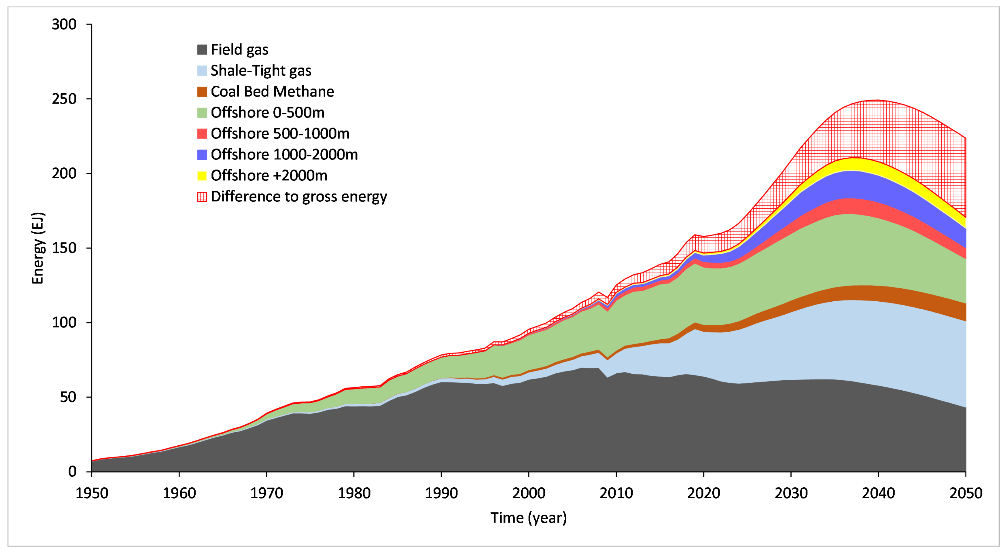
The gross energy peak in gas is expected to take place in 2040, with a magnitude of 249 EJ. The increase rate prior to the peak is estimated to 4.3 EJ/year, and the post-peak decrease rate to 2.55 EJ/year. The decrease/increase rates ratio equals 0.59, which highlights the fact that gas is produced faster before the peak than after. The net-energy peak of gas is predicted for 2037 to be in the order of 210 EJ. The energy necessary for gas production at the peak, therefore, represent 40 EJ, or 15.9% of the gross energy peak magnitude. The net-energy increase rate reaches 3.5 EJ/year, and the decrease rate 3.1 EJ/year. The net-energy decrease/increase ratio is 0.92, a rise of 54% compared to the gross energy. If the year of the peak and the magnitude matter, this ratio seems to be the most key factor, as it implies that the gas production sector will need important and accelerated energy inputs to keep producing. Finally, the energy contribution over the 1950–2050 period per type of gas is led by field gas (48%), followed by offshore shallow gas (23%) and shale-tight (17%); the rest does not exceed 5% per gas. However, unconventional gases (all gases except onshore field gas and offshore shallow gas) grow in proportion over time to reach about 35% of the total gross energy produced between 2000 and 2050. Figure 1 presents the average net-energy production of gas from 1950 to 2050.

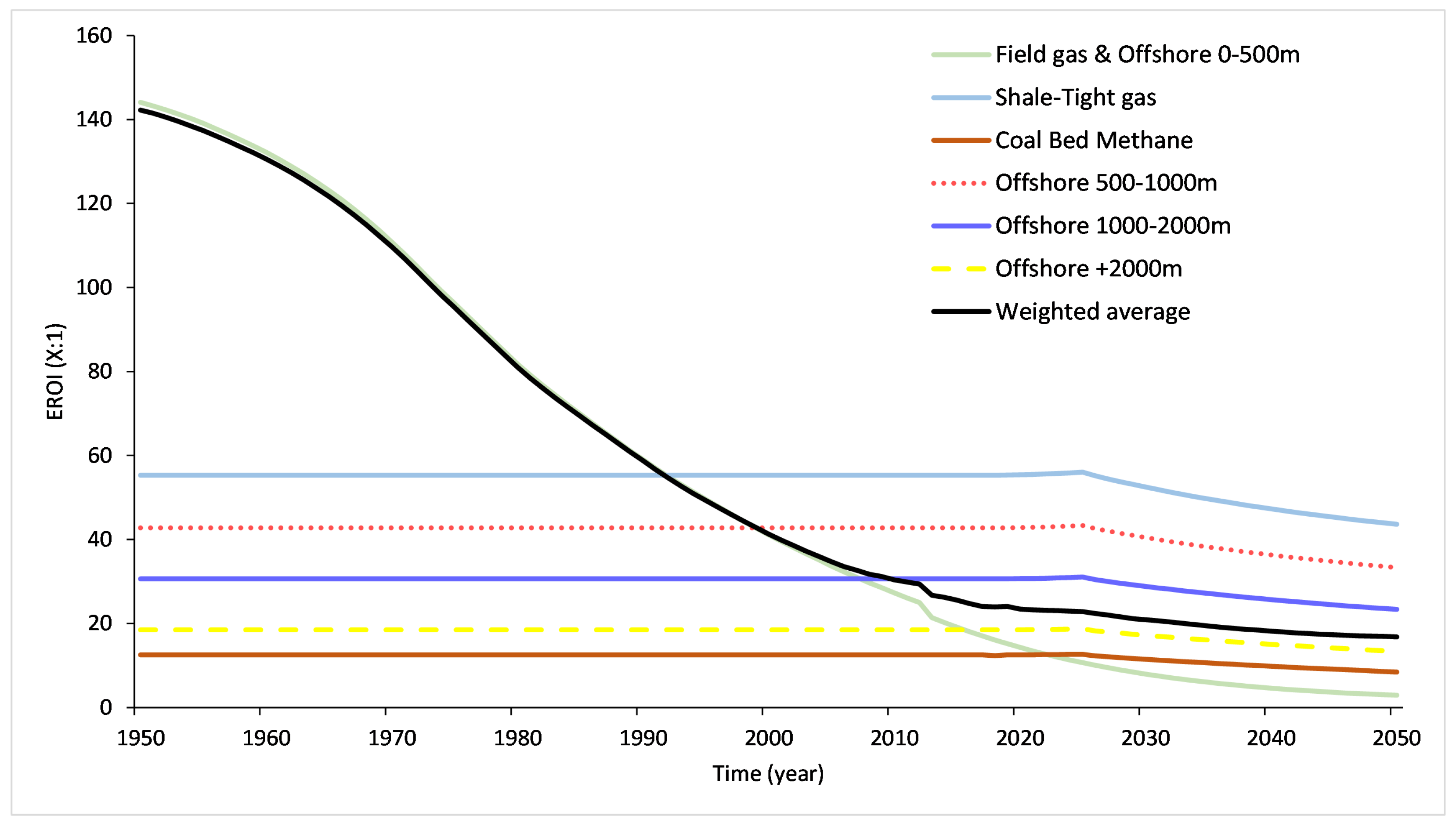
The weighted-average EROI experiences a steady decrease from its initial value of 141.5 to an apparent plateau of 16.8. This reduction is, in large part, due to the decrease in conventional gases’ EROI, which begins to be inferior to: shale-tight gas EROI in 1992, offshore 500–1000 m in 2000, offshore 1000–2000 m in 2008, offshore +2000 m in 2016 and coal bed methane in 2022. Let us note that the drop-off of the conventional gases towards 2012 is linked to the reconciliation of the yearly EROI calculation with the historical and prospective exploitation resource ratios, a parameter used in the functional form definition (we recommend the reader consults the work of Court and Fizaine to clarify the theorized functional forms of EROI). Figure 2 illustrates the evolution of the EROI of all gas types, and the weighted average from 1950 to 2050.

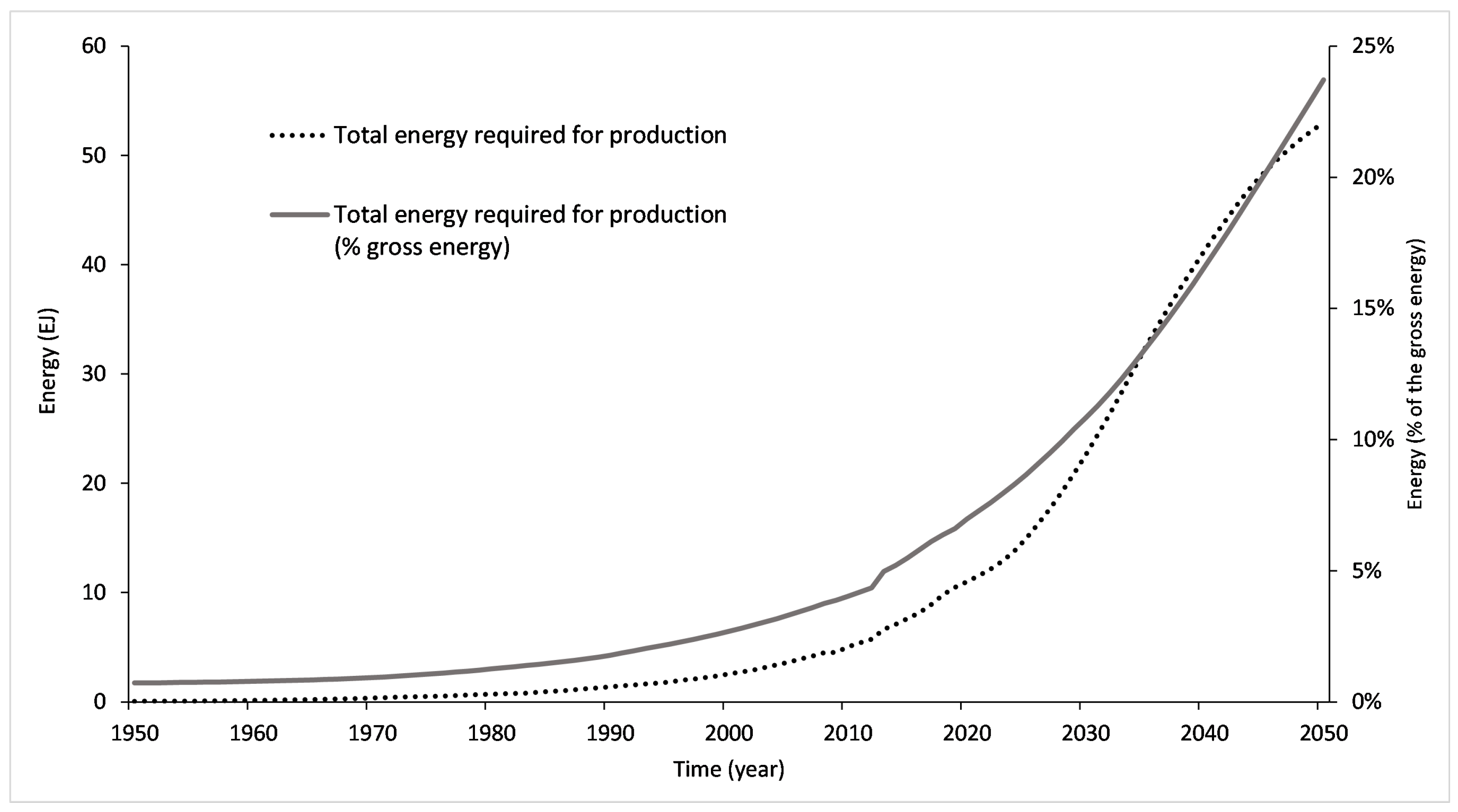
The energy required for the production of gases grows from 1.3 EJ in 1990 to 11 EJ in 2020 and 53 EJ in 2050, showing an exponential increase until the curve starts to flatten from 2040. This respectively represents 1.7%, 6.3% and 23.7% of the gross energy production, as illustrated in Figure 3. In other terms, an amount equivalent to nearly a quarter of the energy production of gases will be necessary in 2050 in order to keep producing. Nevertheless, the precise breakdown by energy sources (electricity, gas itself, etc.) remains to be treated in future research.

3.2. Scenario-Based Sensitivity Analysis

3.2.1. EROI Estimates

As one could expect, reduced EROI estimates induce an earlier peak, but the trend is rather weak (less than two years of difference between the high and low estimates). A more notable variation appears for the net-energy peak magnitude, with a 37 EJ gap between high and low EROIs estimates, which represents 17% of the net-energy peak for the medium estimate hypothesis. The decrease/increase ratio is the output the most sensible for the estimate, with a difference of 0.4 between the high and low estimates, which represents 44% of the rate for the medium estimate.

Table 6. Dependence of the results on the EROI estimate hypotheses (high, medium, low).

Output Assessed	High	Medium	Low
Peak year	2038	2037	2036
Peak magnitude	226.4	214.7	189.5
Decrease/increase ratio	0.8	0.9	1.2

summarizes the dependence of the outputs on EROI estimate hypotheses.

3.2.2. Dynamic Functions

All the dynamic functions hypotheses present similar features in term of outputs. Taking dynamic functions into account lowers the peak magnitude but does not impact the peak year. However, it has a relative effect on the decrease/increase rates ratio. More precisely, the constant, increase and decrease function (named “constant, bump”) shows little to no difference when compared with other functions. However, these results would benefit from being re-examined with a greater diversity of decline functions, and should be put into perspective with regard to the important contribution of onshore field and offshore shallow gases that have yearly values.

Table 7. Dependence of the results on the decline year hypotheses.

Output Assessed	Constant	Constant, Decrease	Constant, Bump
Peak year	2037	2037	2037
Peak magnitude	211.8	210.0	211.5
Decrease/increase ratio	0.9	1.0	0.9

summarizes the dependence of the outputs on the different dynamic functions’ hypotheses.

3.3. Robustness of the Results

In order to analyze the robustness of the results, we constructed a 3-level robustness scale. “0” indicates that the evaluation of the net-energy does not give a significant qualitative and quantitative variation compared to the gross energy (when the difference between gross and net-energy output values is less than half of the average standard deviation of net-energy), “+” indicates a qualitative significance (when the difference is of the order of the standard deviation) and “++” a qualitative and quantitative significance (when the difference is more than twice the standard deviation).

From this scale, it appears that net-energy is clearly robust for the peak year, the peak magnitude and the post-peak energy decrease rate, on both the qualitative and quantitative fronts. It is also qualitatively significant for the pre-peak increase rate and the decrease/increase ratio. Overall, these results testify that, in all likelihood, relative trends are independent of our choice of gross energy data. The results of this robustness evaluation are summarized in

Table 8. Comparison between gross and net-energy outputs to estimate the robustness of the results.

Output Assessed	Gross Energy	Net-Energy	$\left|\frac{{\mathbf{x}}_{\mathbf{gross}}-{\mathbf{x}}_{\mathbf{net},\mathbf{avg}}}{{\mathit{\sigma }}_{\mathbf{net}}}\right|$	Scale
Peak year	2040	2037	3.6	++
Peak magnitude	249	211	2.5	++
Pre-peak increase	4.3	3.4	1.8	+
Post-peak decrease	2.6	3.1	2.5	++
Decrease/increase ratio	0.6	0.9	1.8	+

.

4. Discussion

4.1. Implications for the Low-Carbon Energy Transition

This study uses GlobalShift’s all-gases projection and a panel of standard EROI scenarios to characterize the dynamic evolution of the primary stage net-energy of gas along the transition from conventional to unconventional resources.

We estimate the current energy required to produce gas to be in the order of 11 EJ for 2020, which is equivalent to 6.7% of the gross energy production of gas. We also show that if the weighted-average standard EROI of gas production is set to reach an apparent plateau of 16.7, the energy required to produce gas keeps increasing to reach 53 EJ in 2050, which would represent 23.7% of the gross energy produced by gas at that time. Finally, we point out that our model features are robust on the qualitative side, and, for some, on both on the qualitative and quantitative fronts. This means that the relative trends from our results are, in all likelihood, independent of the choice of gross energy data.

Retrieving the energy necessary for the oil liquid production from Delannoy et al. [81], we estimate the energy necessary for both fossil fuel production to equal 37.4 EJ in 2020. This is equivalent to the aggregated primary energy consumption of France, Germany, United Kingdom and Italy [1]. Moreover, the total amount of energy required for the production of oil and gas can be expected to grow exponentially. Increased energy consumption in the energy production sector can be likened to “energy cannibalism”, i.e., a reduction in the energy available for society’s other needs [83] which itself bears energy security and environmental degradation risks. If we specifically highlight the danger of turning to coal (directly or indirectly) to power the oil and gas industry, the possible use of renewables is not without consequences too, as the production of energy, from whatever source, impacts the environment. Low and diminishing energy returns are, therefore, not only a threat to energy security, but also to the environment itself. We are concerned that both risks might be underestimated and urge energy transition models to adopt a net-energy perspective.

4.2. On the Need of Net-Energy Studies

That said, we feel that the published net energy literature is not sufficiently developed. For instance, interrogations remain on the EROI of renewable and fossil energy sources and their evolution over time [21,84,85]. As discussed by Dale [27], there is significant confusion about the difference between energy return on investment and power return on investment, and not just regarding how to calculate each, but also what they imply. There also appears to be a missing link between economic, financial and net energy indicators, and how energy return can or cannot constrain future development in the long run [86,87,88,89]. We, therefore, believe that the debate would strongly benefit from more precise assessments of static and dynamic net energy ratios, including EROI and PROI, for a wide array of energy sources. We thus call for a new wave of net energy studies, possibly in line with exergy economics (https://exergyeconomics.wordpress.com/, accessed on 15 July 2021).

4.3. Limitations and Future Work

Our study suffers from a number of limitations, discussed here. First of all, our analysis relies on the use of external gross energy data bought from GlobalShift, which, as for every future scenario, will, in all likeliness, not depict the reality. However, we have pointed out that because the results obtained here should be qualitatively correct, and, in all likelihood, semi-quantitatively correct in net vs. gross relative difference. Furthermore, one should note that the objective of this article is to estimate the impact of the net-energy perspective against the gross energy, rather than guess a peak date and magnitude. Secondly, our EROI scenarios are based on desk-research of the published resources, which comprises several uncertainties. We have attempted to compensate for them by developing a set of scenarios, which are characterized in a sensitivity analysis. Third, we only focused on standard EROI and did not pay attention to the societal EROI, which could be a more meaningful indicator [36]. However, restraining ourselves to standard EROI has made the EROIs of different gases more easily comparable (the basis of comparison being clearer and closer to physical extraction and other processes, and, therefore, less subject to interpretation).

Improvements to the present study could be carried out in several ways. First, a more precise assessment of how gas-producing countries would react to strong climate-change restrictions in GlobalShift’s model would prove useful to support a faster transition to low-carbon energy sources. Second, the use of more precise EROI estimates or dynamic functions parameters would allow the study to gain in accuracy. Another improvement for EROI would be the use of societal EROI; in this way, net-energy variations along the transition from conventional to unconventional gases would be assessed for the entire value chain, but at the cost of increased uncertainty.

5. Conclusions

The industrial society can be likened to a thermodynamic system that profoundly relies on abundant and cheap energy intakes such as oil or gas to thrive [90]. However, the rapid growth in use of non-renewable fossil fuels has undermined their future availability, and a shift from conventional sources to unconventional ones has started.

Such a shift has had considerable effects on the net-energy supply of gas. For instance, we find that the total energy needed for the gas production continually increases, from a proportion equivalent to 6.3% of the gross energy produced from gas at present, to 23.7% in 2050. We thus foresee an important use of energy to produce gas in the future, a phenomenon relating to “energy cannibalism” [83], which bears energy security and environmental degradation risks. Low and diminishing energy returns are, therefore, not only a threat to energy security but also to the environment itself. Although our approach is subject to various uncertainties, the gaps between net and gross energy are statistically significant, to uphold the fact that our results are qualitatively and, to some extent, quantitatively robust. In other terms, this means that the relative trends from our results are, in all likelihood, independent of the choice of gross energy data.

Our findings highlight the necessity to see the energy transition from a net-energy perspective, not only for energy security concerns but also for the multiplication of environmental damages that a low-energy-yield energy production is likely to drive. We thus call for the energy transition debate to adopt a net-energy analysis, and for a new wave of net energy ratios studies, including EROI and PROI, to consider wise energy consumption and its environmental impacts.

References

- Bristish Petroleum Statistical Review of World Energy. 2020. Available online: https://www.bp.com/content/dam/bp/business-sites/en/global/corporate/pdfs/news-and-insights/speeches/bp-stats-review-2019-bob-dudley-speech.pdf (accessed on 15 July 2021).
- Costa, D.; Jesus, J.; Branco, D.; Danko, A.; Fiúza, A. Extensive review of shale gas environmental impacts from scientific literature (2010–2015). Environ. Sci. Pollut. Res. 2017, 24, 14579–14594. [Google Scholar] [CrossRef]
- IPCC. Climate Change 2021 The Physical Science Basis. In Intergovernmental Panel on Climate Change, Working Group I Contribution to the Sixth Assessment Report; IPCC: Geneva, Switzerland, 2021. [Google Scholar]
- Loftus, P.J.; Cohen, A.M.; Long, J.C.S.; Jenkins, J.D. A critical review of global decarbonization scenarios: What do they tell us about feasibility? Wiley Interdiscip. Rev. Clim. Chang. 2014, 6, 93–112. [Google Scholar] [CrossRef]
- Heard, B.; Brook, B.; Wigley, T.; Bradshaw, C. Burden of proof: A comprehensive review of the feasibility of 100% renewable-electricity systems. Renew. Sustain. Energy Rev. 2017, 76, 1122–1133. [Google Scholar] [CrossRef]
- Smil, V. Energy Transitions: Global and National Perspectives; Praeger, an Imprint of ABC-CLIO, LLC: Santa Barbara, CA, USA, 2017. [Google Scholar]
- Napp, T.; Bernie, D.; Thomas, R.; Lowe, J.; Hawkes, A.; Gambhir, A. Exploring the Feasibility of Low-Carbon Scenarios Using Historical Energy Transitions Analysis. Energies 2017, 10, 116. [Google Scholar] [CrossRef] [Green Version]
- Brown, T.; Bischof-Niemz, T.; Blok, K.; Breyer, C.; Lund, H.; Mathiesen, B. Response to ‘Burden of proof: A comprehensive review of the feasibility of 100% renewable-electricity systems’. Renew. Sustain. Energy Rev. 2018, 92, 834–847. [Google Scholar] [CrossRef]
- King, L.C.; van den Bergh, J.C.J.M. Implications of net energy-return-on-investment for a low-carbon energy transition. Nat. Energy 2018, 3, 334–340. [Google Scholar] [CrossRef] [Green Version]
- Sers, M.R.; Victor, P.A. The Energy-emissions Trap. Ecol. Econ. 2018, 151, 10–21. [Google Scholar] [CrossRef]
- Vidal, O.; Boulzec, H.L.; François, C. Modelling the material and energy costs of the transition to low-carbon energy. EPJ Web Conf. 2018, 189, 00018. [Google Scholar] [CrossRef] [Green Version]
- Jewell, J.; Cherp, A. On the political feasibility of climate change mitigation pathways: Is it too late to keep warming below 1.5 °C? WIREs Clim. Chang. 2019, 11, e621. [Google Scholar] [CrossRef] [Green Version]
- Capellán-Pérez, I.; de Blas, I.; Nieto, J.; de Castro, C.; Miguel, L.J.; Carpintero, Ó.; Mediavilla, M.; Lobejón, L.F.; Ferreras-Alonso, N.; Rodrigo, P.; et al. MEDEAS: A new modeling framework integrating global biophysical and socioeconomic constraints. Energy Environ. Sci. 2020, 13, 986–1017. [Google Scholar] [CrossRef]
- Nieto, J.; Carpintero, Ó.; Miguel, L.J.; de Blas, I. Macroeconomic modelling under energy constraints: Global low carbon transition scenarios. Energy Policy 2020, 137, 111090. [Google Scholar] [CrossRef] [Green Version]
- Moriarty, P.; Honnery, D. Feasibility of a 100% Global Renewable Energy System. Energies 2020, 13, 5543. [Google Scholar] [CrossRef]
- Dupont, E.; Germain, M.; Jeanmart, H. Feasibility and Economic Impacts of the Energy Transition. Sustainability 2021, 13, 5345. [Google Scholar] [CrossRef]
- Smil, V. Natural Gas: Fuel for the 21st Century; John Wiley and Sons Ltd.: Hoboken, NJ, USA, 2015. [Google Scholar]
- Gürsan, C.; de Gooyert, V. The systemic impact of a transition fuel: Does natural gas help or hinder the energy transition? Renew. Sustain. Energy Rev. 2021, 138, 110552. [Google Scholar] [CrossRef]
- Murphy, D.J. The implications of the declining energy return on investment of oil production. Philos. Trans. R. Soc. A Math. Phys. Eng. Sci. 2014, 372, 20130126. [Google Scholar] [CrossRef] [PubMed]
- Carbajales-Dale, M.; Barnhart, C.J.; Brandt, A.R.; Benson, S.M. A better currency for investing in a sustainable future. Nat. Clim. Chang. 2014, 4, 524–527. [Google Scholar] [CrossRef]
- Rana, R.L.; Lombardi, M.; Giungato, P.; Tricase, C. Trends in Scientific Literature on Energy Return Ratio of Renewable Energy Sources for Supporting Policymakers. Adm. Sci. 2020, 10, 21. [Google Scholar] [CrossRef] [Green Version]
- Hall, C. Migration and Metabolism in a Temperate Stream Ecosystem. Ecology 1972, 53, 585–604. [Google Scholar] [CrossRef]
- Hall, C. Energy Return on Investment; Springer International Publishing: Berlin/Heidelberg, Germany, 2017. [Google Scholar] [CrossRef]
- Raugei, M. Net energy analysis must not compare apples and oranges. Nat. Energy 2019, 4, 86–88. [Google Scholar] [CrossRef]
- Buchanan, M. Energy costs. Nat. Phys. 2019, 15, 520. [Google Scholar] [CrossRef]
- Murphy, D.J.; Hall, C.A.; Dale, M.; Cleveland, C. Order from Chaos: A Preliminary Protocol for Determining the EROI of Fuels. Sustainability 2011, 3, 1888–1907. [Google Scholar] [CrossRef] [Green Version]
- Carbajales-Dale, M. When is EROI Not EROI? BioPhysical Econ. Resour. Qual. 2019, 4, 1–4. [Google Scholar] [CrossRef] [Green Version]
- Hall, C.A.; Lambert, J.G.; Balogh, S.B. EROI of different fuels and the implications for society. Energy Policy 2014, 64, 141–152. [Google Scholar] [CrossRef] [Green Version]
- White, E.; Kramer, G.J. The Changing Meaning of Energy Return on Investment and the Implications for the Prospects of Post-fossil Civilization. ONE Earth 2019, 1, 416–422. [Google Scholar] [CrossRef]
- Court, V.; Fizaine, F. Long-Term Estimates of the Energy-Return-on-Investment (EROI) of Coal, Oil, and Gas Global Productions. Ecol. Econ. 2017, 138, 145–159. [Google Scholar] [CrossRef]
- Gagnon, N.; Hall, C.; Brinker, L. A Preliminary Investigation of Energy Return on Energy Investment for Global Oil and Gas Production. Energies 2009, 2, 490–503. [Google Scholar] [CrossRef]
- Brandt, A.R.; Sun, Y.; Bharadwaj, S.; Livingston, D.; Tan, E.; Gordon, D. Energy Return on Investment (EROI) for Forty Global Oilfields Using a Detailed Engineering-Based Model of Oil Production. PLoS ONE 2015, 10, e0144141. [Google Scholar] [CrossRef] [Green Version]
- Dale, M.; Krumdieck, S.; Bodger, P. Net energy yield from production of conventional oil. Energy Policy 2011, 39, 7095–7102. [Google Scholar] [CrossRef]
- Tollefson, J. Is the 2 °C world a fantasy? Nature 2015, 527, 436–438. [Google Scholar] [CrossRef] [Green Version]
- Raftery, A.E.; Zimmer, A.; Frierson, D.M.W.; Startz, R.; Liu, P. Less than 2 °C warming by 2100 unlikely. Nat. Clim. Chang. 2017, 7, 637–641. [Google Scholar] [CrossRef]
- Brockway, P.E.; Owen, A.; Brand-Correa, L.I.; Hardt, L. Estimation of global final-stage energy-return-on-investment for fossil fuels with comparison to renewable energy sources. Nat. Energy 2019, 4, 612–621. [Google Scholar] [CrossRef] [Green Version]
- Capellán-Pérez, I.; de Castro, C.; González, L.J.M. Dynamic Energy Return on Energy Investment (EROI) and material requirements in scenarios of global transition to renewable energies. Energy Strategy Rev. 2019, 26, 100399. [Google Scholar] [CrossRef]
- Gately, M. The EROI of U.S. offshore energy extraction: A net energy analysis of the Gulf of Mexico. Ecol. Econ. 2007, 63, 355–364. [Google Scholar] [CrossRef]
- Guilford, M.C.; Hall, C.A.; O’Connor, P.; Cleveland, C.J. A New Long Term Assessment of Energy Return on Investment (EROI) for U.S. Oil and Gas Discovery and Production. Sustainability 2011, 3, 1866–1887. [Google Scholar] [CrossRef] [Green Version]
- Moerschbaecher, M.; Day, J.W., Jr. Ultra-Deepwater Gulf of Mexico Oil and Gas: Energy Return on Financial Investment and a Preliminary Assessment of Energy Return on Energy Investment. Sustainability 2011, 3, 2009–2026. [Google Scholar] [CrossRef] [Green Version]
- Freise, J. The EROI of Conventional Canadian Natural Gas Production. Sustainability 2011, 3, 2080–2104. [Google Scholar] [CrossRef] [Green Version]
- Sell, B.; Murphy, D.; Hall, C.A. Energy Return on Energy Invested for Tight Gas Wells in the Appalachian Basin, United States of America. Sustainability 2011, 3, 1986–2008. [Google Scholar] [CrossRef] [Green Version]
- Poisson, A.; Hall, C. Time Series EROI for Canadian Oil and Gas. Energies 2013, 6, 5940–5959. [Google Scholar] [CrossRef] [Green Version]
- Aucott, M.L.; Melillo, J.M. A Preliminary Energy Return on Investment Analysis of Natural Gas from the Marcellus Shale. J. Ind. Ecol. 2013, 17, 668–679. [Google Scholar] [CrossRef]
- Dale, A.T.; Khanna, V.; Vidic, R.D.; Bilec, M.M. Process Based Life-Cycle Assessment of Natural Gas from the Marcellus Shale. Environ. Sci. Technol. 2013, 47, 5459–5466. [Google Scholar] [CrossRef]
- Nogovitsyn, R.; Sokolov, A. Preliminary Calculation of the EROI for the Production of Gas in Russia. Sustainability 2014, 6, 6751–6765. [Google Scholar] [CrossRef] [Green Version]
- Yaritani, H.; Matsushima, J. Analysis of the Energy Balance of Shale Gas Development. Energies 2014, 7, 2207–2227. [Google Scholar] [CrossRef] [Green Version]
- Moeller, D.; Murphy, D. Net Energy Analysis of Gas Production from the Marcellus Shale. BioPhysical Econ. Resour. Qual. 2016, 1, 1–13. [Google Scholar] [CrossRef]
- Siažik, J.; Malcho, M.; Čaja, A. Calculation of the EROIE coefficient for natural gas hydrates in laboratory conditions. AIP Conf. Proc. 2017, 020036. [Google Scholar] [CrossRef] [Green Version]
- de Luna Marques, A.; de Queiroz Fernandes Araújo, O.; Cammarota, M.C. Biogas from microalgae: An overview emphasizing pretreatment methods and their energy return on investment (EROI). Biotechnol. Lett. 2018, 41, 193–201. [Google Scholar] [CrossRef] [PubMed]
- Hu, Y.; Hall, C.A.; Wang, J.; Feng, L.; Poisson, A. Energy Return on Investment (EROI) of China’s conventional fossil fuels: Historical and future trends. Energy 2013, 54, 352–364. [Google Scholar] [CrossRef]
- Kong, Z.; Dong, X.; Liu, G. Coal-based synthetic natural gas vs. imported natural gas in China: A net energy perspective. J. Clean. Prod. 2016, 131, 690–701. [Google Scholar] [CrossRef]
- Kong, Z.Y.; Dong, X.C.; Shao, Q.; Wan, X.; Tang, D.L.; Liu, G.X. The potential of domestic production and imports of oil and gas in China: An energy return on investment perspective. Pet. Sci. 2016, 13, 788–804. [Google Scholar] [CrossRef] [Green Version]
- Lior, N. Exergy, Energy, and Gas Flow Analysis of Hydrofractured Shale Gas Extraction. J. Energy Resour. Technol. 2016, 138, 1–14. [Google Scholar] [CrossRef] [Green Version]
- Wang, J.L.; Feng, J.X.; Bentley, Y.; Feng, L.Y.; Qu, H. A review of physical supply and EROI of fossil fuels in China. Pet. Sci. 2017, 14, 806–821. [Google Scholar] [CrossRef] [Green Version]
- Wang, J.; Liu, M.; McLellan, B.C.; Tang, X.; Feng, L. Environmental impacts of shale gas development in China: A hybrid life cycle analysis. Resour. Conserv. Recycl. 2017, 120, 38–45. [Google Scholar] [CrossRef]
- Kong, Z.Y.; Dong, X.C.; Lu, X.; Wan, X. Energy return on investment, energy payback time, and greenhouse gas emissions of coal seam gas (CSG) production in China: A case of the Fanzhuang CSG project. Pet. Sci. 2017, 15, 185–199. [Google Scholar] [CrossRef] [Green Version]
- Kong, Z.; Jiang, Q.; Dong, X.; Wang, J.; Wan, X. Estimation of China’s production efficiency of natural gas hydrates in the South China Sea. J. Clean. Prod. 2018, 203, 1–12. [Google Scholar] [CrossRef]
- Kong, Z.; Lu, X.; Dong, X.; Jiang, Q.; Elbot, N. Re-evaluation of energy return on investment (EROI) for China’s natural gas imports using an integrative approach. Energy Strategy Rev. 2018, 22, 179–187. [Google Scholar] [CrossRef]
- Cheng, C.; Wang, Z.; Wang, J.; Liu, M.; Ren, X. Domestic oil and gas or imported oil and gas – An energy return on investment perspective. Resour. Conserv. Recycl. 2018, 136, 63–76. [Google Scholar] [CrossRef] [Green Version]
- Chen, Y.; Feng, L.; Tang, S.; Wang, J.; Huang, C.; Höök, M. Extended-exergy based energy return on investment method and its application to shale gas extraction in China. J. Clean. Prod. 2020, 260, 120933. [Google Scholar] [CrossRef]
- Smith, M.R. Forecasting Oil & Gas Supply And Activity. Oil Age 2015, 1, 35–58. [Google Scholar]
- Maggio, G.; Cacciola, G. When will oil, natural gas, and coal peak? Fuel 2012, 98, 111–123. [Google Scholar] [CrossRef]
- Mohr, S.; Wang, J.; Ellem, G.; Ward, J.; Giurco, D. Projection of world fossil fuels by country. Fuel 2015, 141, 120–135. [Google Scholar] [CrossRef]
- DNV. Energy Transition Outlook; Det Norske Veritas: Oslo, Norway, 2020. [Google Scholar]
- GEFC. Global Gas Outlook 2050 Synopsis. Gas Export. Ctries. Forum 2021. Available online: https://www.gecf.org/insights/global-gas-outlook?d=2021&p=1 (accessed on 15 July 2021).
- IEA. World Energy Outlook; International Energy Agency: Paris, France, 2020. [Google Scholar]
- Tan, L.; Zuo, L.; Wang, B. Methods of Decline Curve Analysis for Shale Gas Reservoirs. Energies 2018, 11, 552. [Google Scholar] [CrossRef] [Green Version]
- Kontorovich, A.; Epov, M.; Eder, L. Long-term and medium-term scenarios and factors in world energy perspectives for the 21st century. Russ. Geol. Geophys. 2014, 55, 534–543. [Google Scholar] [CrossRef]
- Laherrère, J. Club de Nice XVIII forum 1er décembre 2020. Bilan et perspectives énergétiques mondiales. Evolution de l’énergie: Pics passés, présents et futurs. ASPO France 2020. Available online: https://aspofrance.files.wordpress.com/2020/12/jean-laherrere-nice2020-cor6dec-presentation.pdf (accessed on 15 July 2021).
- Valero, A.; Valero, A. Physical geonomics: Combining the exergy and Hubbert peak analysis for predicting mineral resources depletion. Resour. Conserv. Recycl. 2010, 54, 1074–1083. [Google Scholar] [CrossRef]
- Wang, J.; Bentley, Y. Modelling world natural gas production. Energy Rep. 2020, 6, 1363–1372. [Google Scholar] [CrossRef]
- Kober, T.; Schiffer, H.W.; Densing, M.; Panos, E. Global energy perspectives to 2060—WEC’s World Energy Scenarios 2019. Energy Strategy Rev. 2020, 31, 100523. [Google Scholar] [CrossRef]
- Zou, C.; Zhao, Q.; Zhang, G.; Xiong, B. Energy revolution: From a fossil energy era to a new energy era. Nat. Gas Ind. B 2016, 3, 1–11. [Google Scholar] [CrossRef] [Green Version]
- EIA. Annual Energy Outlook; Energy Information Administration: Washington, DC, USA, 2021.
- Azari, M.; Hamza, F.; Hadibeik, H.; Ramakrishna, S. Well-Testing Challenges in Unconventional and Tight Gas Reservoirs. In Proceedings of the SPE Western Regional Meeting, Garden Grove, CA, USA, 26 April 2018. [Google Scholar] [CrossRef]
- OPEC. World Oil Outlook 2045; Organization of the Petroleum Exporting Countries: Vienna, Austria, 2020. [Google Scholar]
- IEA. Natural Gas Information: Database Documentation; International Energy Agency: Paris, France, 2021. [Google Scholar]
- McGlade, C.; Ekins, P. The geographical distribution of fossil fuels unused when limiting global warming to 2 °C. Nature 2015, 517, 187–190. [Google Scholar] [CrossRef]
- Jones, J. Energy-Return-On-Energy-Invested (EROEI) For Crude Oil and Other Sources of Energy. J. Pet. Environ. Biotechnol. 2013, 4, 150. [Google Scholar] [CrossRef] [Green Version]
- Delannoy, L.; Longaretti, P.Y.; Murphy, D.J.; Prados, E. Peak oil and the low-carbon energy transition: A net-energy perspective. Appl. Energy 2021. submitted. [Google Scholar]
- Heun, M.K.; de Wit, M. Energy return on (energy) invested (EROI), oil prices, and energy transitions. Energy Policy 2012, 40, 147–158. [Google Scholar] [CrossRef]
- Pearce, J.M. Thermodynamic limitations to nuclear energy deployment as a greenhouse gas mitigation technology. Int. J. Nucl. Gov. Econ. Ecol. 2008, 2, 113. [Google Scholar] [CrossRef]
- de Castro, C.; Capellán-Pérez, I. Standard, Point of Use, and Extended Energy Return on Energy Invested (EROI) from Comprehensive Material Requirements of Present Global Wind, Solar, and Hydro Power Technologies. Energies 2020, 13, 3036. [Google Scholar] [CrossRef]
- Wang, C.; Zhang, L.; Chang, Y.; Pang, M. Energy return on investment (EROI) of biomass conversion systems in China: Meta-analysis focused on system boundary unification. Renew. Sustain. Energy Rev. 2021, 137, 110652. [Google Scholar] [CrossRef]
- King, C.W.; Hall, C.A. Relating Financial and Energy Return on Investment. Sustainability 2011, 3, 1810–1832. [Google Scholar] [CrossRef] [Green Version]
- King, C.; Maxwell, J.; Donovan, A. Comparing World Economic and Net Energy Metrics, Part 1: Single Technology and Commodity Perspective. Energies 2015, 8, 12949–12974. [Google Scholar] [CrossRef] [Green Version]
- King, C.; Maxwell, J.; Donovan, A. Comparing World Economic and Net Energy Metrics, Part 2: Total Economy Expenditure Perspective. Energies 2015, 8, 12975–12996. [Google Scholar] [CrossRef] [Green Version]
- King, C. Comparing World Economic and Net Energy Metrics, Part 3: Macroeconomic Historical and Future Perspectives. Energies 2015, 8, 12997–13020. [Google Scholar] [CrossRef] [Green Version]
- Smil, V. Energy and Civilization; MIT Press Ltd.: Cambridge, MA, USA, 2018. [Google Scholar]
Figure 1.
Average gas net-energy production from 1950 to 2050, compared to the gross energy.
Figure 2.
Evolution of the EROI of all gas types, and the weighted average from 1950 to 2050.
Figure 3.
Evolution of energy required to produce gases from 1950 to 2050.