Reinforcement Learning for Energy-Storage Systems in Grid-Connected Microgrids: An Investigation of Online vs. Offline Implementation

Abstract

Grid-connected microgrids consisting of renewable energy sources, battery storage, and load require an appropriate energy management system that controls the battery operation. Traditionally, the operation of the battery is optimised using 24 h of forecasted data of load demand and renewable energy sources (RES) generation using offline optimisation techniques, where the battery actions (charge/discharge/idle) are determined before the start of the day. Reinforcement Learning (RL) has recently been suggested as an alternative to these traditional techniques due to its ability to learn optimal policy online using real data. Two approaches of RL have been suggested in the literature viz. offline and online. In offline RL, the agent learns the optimum policy using predicted generation and load data. Once convergence is achieved, battery commands are dispatched in real time. This method is similar to traditional methods because it relies on forecasted data. In online RL, on the other hand, the agent learns the optimum policy by interacting with the system in real time using real data. This paper investigates the effectiveness of both the approaches. White Gaussian noise with different standard deviations was added to real data to create synthetic predicted data to validate the method. In the first approach, the predicted data were used by an offline RL algorithm. In the second approach, the online RL algorithm interacted with real streaming data in real time, and the agent was trained using real data. When the energy costs of the two approaches were compared, it was found that the online RL provides better results than the offline approach if the difference between real and predicted data is greater than 1.6%.

1. Introduction

Grid-connected microgrids are becoming the main building blocks of smart grids. They facilitate the vast deployment and better utilisation of RES, reduce stress on the existing power grid, and provide consumers with uninterrupted power supply. The main aim for any Energy Management System (EMS) for grid-connected microgrids is to reduce operational costs by reducing the cost of power imported from the grid. This is achieved by controlling the Battery Energy Storage System (BESS) to store power when RES generation is higher than load demand and release power when it is less than the load demand. However, BESS capacity is finite and hence, depending on the battery size, imported power from the grid is likely to be used. Therefore, grid tariffs, which can vary during the day, must be taken into account when deciding charging and discharging commands. In addition, the feed-in tariff can also be available to enable consumers or prosumers to sell their excess power to the grid [1]. These factors demonstrate the need for an intelligent optimisation method. However, due to the lack of information regarding future generation and load profiles, this presents a challenge for EMS.

Inspired by the classical economic dispatch of power systems, various studies have suggested different optimisation techniques to plan, schedule, and control the BESS in grid-connected microgrids. These studies have formulated the operation of the BESS as a dispatch optimisation problem and solved it using Linear Programming (LP) [2,3], Mixed Integer Programming (MIP) [4], Mixed-Integer Linear Programming (MILP) [5,6,7], and Mixed-Integer Nonlinear Programming (MINLP) [8,9]. In Chen et al. [2], a general algebraic modelling system (GAMS) was developed and solved by CPLEX solver and then tested in a physical system based in Taiwan. The study compared two models to determine the impact of energy storage on optimal scheduling. The first model consisted of thermal and electrical loads and a CHP unit. The second model used additional thermal and electrical storage. Both models used in this work relied on the prediction of load profiles. In Luna et al. [5], the model reflects a deterministic problem that promotes self-consumption based on 24 h look-ahead forecast data. The microgrid consists of a supervisory control stage that compensates for any mismatch between the offline scheduling process and the real-time microgrid operation. In Li et al. [7], the microgrid optimisation problem is formalised using a general algebraic modelling system (GAMS) via a discretised step transformation (DST) approach and finally solved using the CPLEX solver. This paper proposes a new optimal scheduling mode by modelling the uncertainty of spinning reserves provided by energy storage with probabilistic constraints. These achievements are highly dependent on the proper estimation of spinning reserves, which is a big challenge while working on a real system. In Mosa and Ali [9], the MINLP algorithm was used to reduce the operational cost of a DC microgrid consisting of a photovoltaic (PV), fuel cell (FC), micro turbine (MT), diesel generator (DE), and battery/BESS. This study uses Egyptian grid load profiles over four seasons of the year based on the prediction.

The above traditional approaches require a detailed and accurate mathematical model of the system, while some of them require the linearisation of the system. In addition, previous knowledge of future RES generation and load demand over a period is required as an input to the optimisation problem. The accuracy of the prediction may affect the accuracy of the BESS operation. Therefore, different forecasting algorithms that can handle the stochastic nature of load demand and RES have been suggested in the literature. These algorithms are designed to forecast short (daily), medium (seasonal), and long (yearly) load demand and availability of RES. Most advanced forecasting algorithms include Artificial Neural Networks (ANN), dynamic programming (DP)-based optimisation, and fuzzy logic by considering the weather conditions. Although forecasting techniques vary within the vast amount of existing literature [10,11,12,13,14,15,16,17,18], the most common objective of these techniques is to decrease the forecasting error by better modelling the uncertainties in real time. Although forecasting algorithms have improved in recent years, it is still challenging to predict the future load demand and availability of RES with minimum error, especially if the decision making is implemented in real time.

Recent studies [19,20,21,22,23,24,25,26] have introduced reinforcement learning as a potential solution for the optimal operation of BESS due to its ability to develop an optimal policy online. In RL, an agent interacts with the surrounding environment and develops an optimal policy for taking the right action after exploring its state. The agent takes the action to maximise a future accumulative reward. The main advantage for RL over traditional methods is that it does not need any model of the environment and it can learn the optimum policy in real time. Yoldas et al. [27] used the MINLP technique guided by a Q-learning algorithm to decrease the daily energy cost and emission of harmful gases simultaneously. Performance comparisons were made using only conventional Q-learning. The result showed an approximately 1.2% reduction of the daily operational costs associated with the proposed technique over conventional Q-learning approaches.

There are two main types of online RL algorithms: off-policy and on-policy. In off-policy methods (e.g., Q-learning), the action-valued function is approximated independently of the policy being followed. Conversely, in on-policy approaches, e.g., in state–action–reward–state–action (SARSA), the action-valued function is continuously updated according to the developed policy, which makes it harder to converge [28]. Whereas with off-policy RL, the agent does not need to follow any specific policy and in fact could even act randomly, on-policy schemes rely on the policy that is being established. Despite the possibly random behaviour, off-policy methods, including the Q-learning algorithm, can converge onto the optimal policy independent on the policy employed during exploration [29]. On the other hand, offline, or data-driven RL develops the policy on pre-collected data. Once the policy is developed, it is deployed to control the system. The policy is not updated by interacting with the system in real time. Offline learning, such as batch RL and other conventional techniques such as MILP, MINLP, and LP algorithms, work with data in bulk. Therefore, the uncertainty of some unknown variables such as load demand and PV profiles make these offline methods more challenging because the training is done on forecasted and not real data. Conventionally, offline learning algorithms need to be re-run from scratch in order to learn from modified or new data.

In Mbuwir et al. [19], the authors proposed batch reinforcement learning, offline RL, to solve the optimisation of the microgrid problem in order to achieve a cost-efficient solution. The goal was to find or statistically learn the pattern of the best control policy from the training data (previous year’s load and PV profiles) in the form of several smaller batches (sets) and then use this policy on the current environment in real time. When the batch RL was compared to the MILP approach, it was shown to be 19% less efficient than MILP. Kuznetsova et al. [30] developed a two-step-ahead RL algorithm to cut down utility bills by learning the stochastic behaviour of the environment using RL and then scheduling the battery two hours ahead from the current time. RL trains the agent and produces the optimal actions of the battery using forecasted wind and load demand power profiles. Liu et al. [20] proposed a cooperative RL algorithm for distributed economic dispatch in microgrids. However, the challenge of using forecasted PV and load data, which can affect function approximation, is not addressed in this paper. Jiang and Fei [21], suggested a Q-learning based, economical smart microgrid with two-level hierarchical agents with flexible demand response and distributed energy resource management. The authors claim that the suggested scheme is very effective while satisfying the user’s preference. However, the suggested work requires load demand from the user before scheduling its distributed units and batteries. This can affect the cost optimisation adversely if the user’s demand request changes during real-time operations.

In [22,25,31,32,33,34,35,36,37,38,39,40,41,42,43], shallow and deep neural networks have been suggested to approximate the Q-value function to achieve better optimisation results with shorter convergence time. Low convergence time is also desirable for online applications. Lu et al. [22] used deep RL to develop an energy-trading scheme according to the predicted future renewable energy generation, estimated future power demand, and battery level. This work also depended on forecasted renewable energy power generation. In Bui et al. [25], a double deep neural network (DDQN) was proposed for function approximation of Q-values. The authors claim that this method trains the model faster as compared with a single deep (having one network) RL algorithm. This work also depends on the estimation of future load demand and PV generation. Zhou et al. [24] suggested an algorithm to train the agent in real time using real data profiles instead of forecasted datasets. A fuzzy Q-learning approach is adopted for a system consisting of household users and a local energy pool in which customers are free to trade with the local energy pool and enjoy low-cost renewable energy while avoiding the installation of new energy generation equipment. Another online approach was proposed in Kim et al. [26] in which real-time pricing is used to reduce the system cost. Both Zhou et al. [24] and Kim et al. [26] do not provide information regarding the efficiency of their algorithms with respect to other offline Q-learning techniques. Another study by Kim and Lim [44] applied Q-learning directly in real time. Optimal cost was achieved for the whole year rather than for a single day. In contrast to other offline approaches, this direct online approach trains the agent in real time using real data by moving from one day to another. In the beginning, the agent experience is low; however, as days progress, the agent starts exploiting more actions, and an optimal policy is developed.

The literature reviewed here suggests that offline policies (including RL) require predicted data in order to produce optimal results if the real data is the same as the predicted data, i.e., zero prediction error. The RL online approach, on the other hand, does not rely on predictions and uses real streaming data. However, it is not clear how effective the online RL algorithm is as compared to the offline approaches when the prediction error increases. Motivated by this shortcoming in the existing literature, this paper provides a comprehensive comparison between the two approaches. Using one year of real PV generation and load data obtained from [45], different profiles for predicted data were created by generating random noise with different standard deviations. The noise was added to the real data to create synthetic predicted data. Then, the 24 h of predicted data were used to train the RL agent, and then, the optimised battery command achieved in this process was applied to the real data (offline RL approach). The online RL, on the other hand, interacted with real data in real time. Then, the energy costs of the two approaches were compared to help users make decisions on the most appropriate approach given the accuracy of the available forecasted data. Finally, the case with zero prediction error was considered in the comparison of MINLP versus RL to establish a benchmark between conventional offline approaches versus the offline RL.

2. Energy Management System

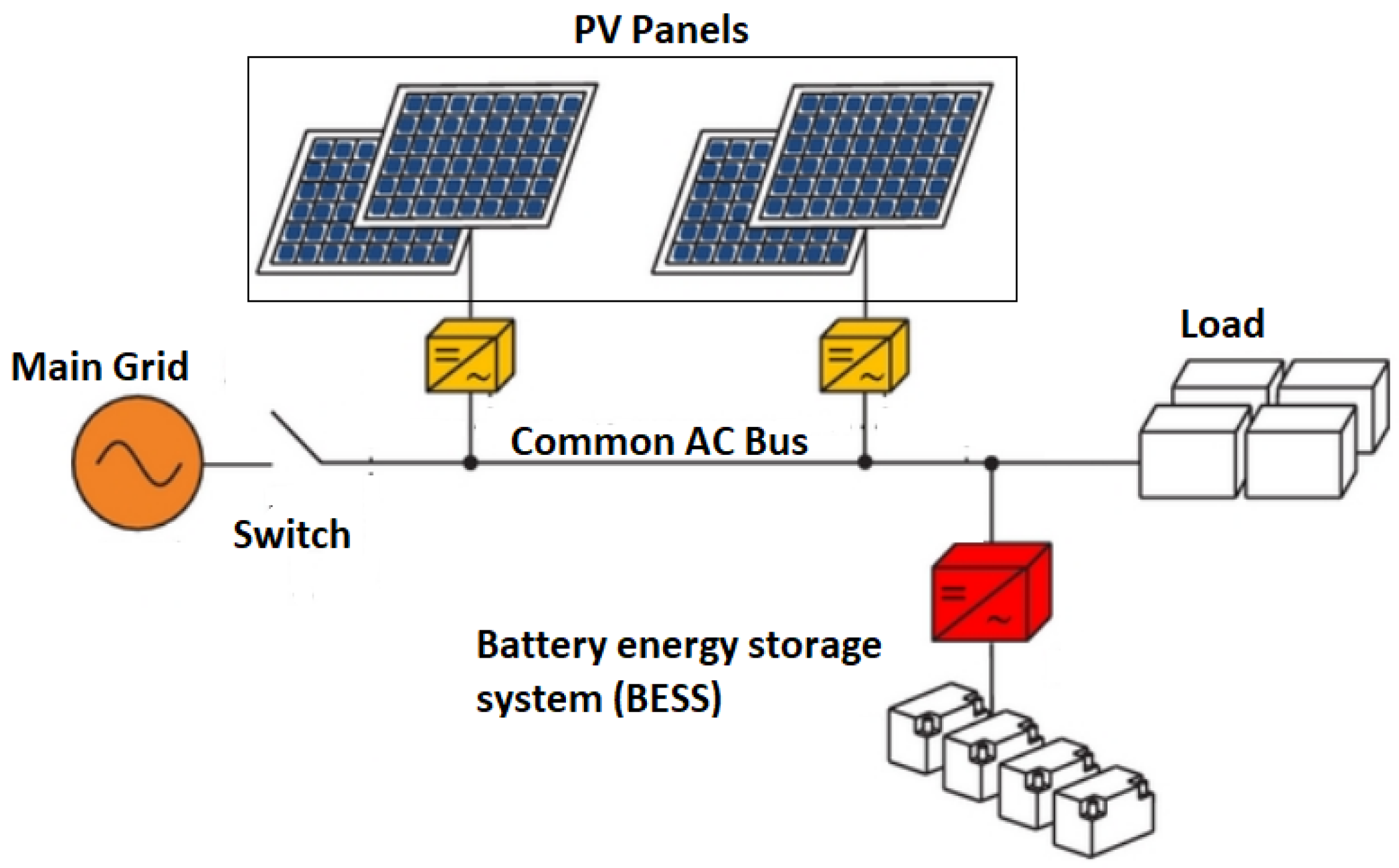
The aim of the EMS is to reduce the cost of the power imported from the grid as shown in Figure 1. Thus, the grid supplies energy only if the RES and BESS do not fulfil the demand, and the time of transfer is chosen in order to minimise the cost. Export of energy to the main grid might also be possible if a feed-in tariff is available. Renewable energy, PV in this study, has a priority to fulfil the load requirement first. If it is not sufficient, then the battery, main grid, or combination of both are used to fulfil the demand. The BESS may charge from the PV directly or charge from or discharge into the main grid if needed. The EMS can make use of different tariff rates within the day by charging the BESS during low-tariff periods and discharging it during high-tariff periods. In this work, a fixed feed-in tariff is assumed, and there are three different tariffs (peak, mid, low) which are assumed to import the energy from the main grid depending on time of the day.

In this paper, an RL algorithm is used to interact with the microgrid and take automated decisions to control the BESS, taking into account a dynamically changing environment characterised by the available PV output, load demand, and the level of battery charge (SOC). The decisions are in the form of actions for the battery to charge, discharge, or remain idle. The recommended actions for the BESS are developed through Q-learning.

2.1. System States

The state space ($S$) is discretised at Δt = 30 min, which suggests that the learning agent captures the information related to the dynamics of the microgrid after the time interval of 30 min. In Equation (1), t represents the time period, which has 48 states in 24 h of a day due to its discretisation every 30 min.

$$s_t=[SOC,\hspace{0.17em}{e}_t^{Net},t]\in S,$$

(1)

where $SOC$, $e_t^{Net}$ are the battery state of charge and net power demand, respectively. The $e_t^{Net}$ is the difference between the load demand and the energy generated by PV such that:

$$e_t^{Net}=e_t^{demand}-e_t^{PV}.$$

(2)

The SOC should be bounded by maximum and minimum limits such that:

$$SO{C}_{\min }\le SOC(t)\le SO{C}_{\max }.$$

(3)

We discretise the state space as shown in Equation (4) below in which the i, j, k indices represent the SOC,$e_t^{Net}$ and t, respectively as:

$${{\displaystyle S}}_{{}_{discrete}}=\left\{{{\displaystyle S}}_{i,j,k}\right\},$$

(4)

where each index in the state space has the following levels: i = 3 levels, j = 2 levels, i.e., positive ($e_t^{Net}\ge e_t^{PV}$) or negative ($e_t^{Net}<e_t^{PV}$), and k = 48 levels. Thus, the total number of states is $48\times 3\times 2=288$.

2.2. Action Space

The action space consists of the charge, discharge, and idle command of the battery such as:

$$A=\left\{\left.a\right|\left(\mathrm{Discharge}, \mathrm{Idle}, \mathrm{Charge}\right)\right\}.$$

(5)

At each time step t, one action is selected from the action space A. If the action “Discharge” is chosen, the battery discharges into the main grid, supplies the load, or both. In case of the action “Idle”, the load demand is fulfilled by the PV source, main grid, or both. If the “Charge” action is selected, the battery is charged from the PV, the grid, or both.

2.3. Backup Controller

In this work, we used a backup controller, which acts as a filter for every control action resulting from the policy π to take care of the practical constraint, such as the inability of the battery to charge or discharge beyond its maximum and minimum SOC level, respectively. In addition, there is a certain limit of battery charging or discharging at time t. For example, if the “Charge” action is selected by the RL agent at time t and one of the discrete states is (${\mathrm{e}}_{\mathrm{t}}^{\mathrm{Net}}>{\mathrm{e}}_{\mathrm{t}}^{\mathrm{PV}}$), then the battery should charge from the main grid up to a certain limit (∆e) defined in

Table 1. Chosen parameters of the microgrid used in this paper.

Name	Values
Total capacity of the battery	12,000 KWh
Max/Min charging rate of battery (∆e)	(2300/2) KW
SOCmax	100%
SOCmin	70%
Initial SOC of the battery (SOC(0))	[min, max]
Time step lenght $(∆t$)	30 min
α, γ, ε	0.5, 0.5, 0.6
Total iterations (Offline)	10,000–15,000

even if the capacity of the battery is more than ∆e. Moreover, if at time t, one of the discrete states is (${\mathrm{e}}_{\mathrm{t}}^{\mathrm{Net}}<{\mathrm{e}}_{\mathrm{t}}^{\mathrm{PV}}$) and the RL agent selects the action “Charge”, the battery will charge from the extra PV available (after fulfilling the load demand) by respecting the charging rate parameter of the battery. If for example the current PV power is more or less than the charging rate of the battery, the battery is charged up to the maximum charging rate (∆e) or current PV power, respectively.

2.4. Reward

The reward function $r(s_t$,$a_t$) is the immediate incentive gained by taking a specific action a at time t in state$s$. The reward function is chosen to minimise the running cost of importing power from the grid and maximise the revenue of selling power to the grid. The cost is calculated every 30 min (as Δt = 30) by multiplying the respective tariff rates, as mentioned in Section 2.5. The reward function is the negative of the cost of imported energy or the cost of exported energy. Hence, the reward function can be formulated as follows:

$$r(s_t,a_t)=\left\{\begin{array}{cc}-P_t^{grid}\times \Delta t\times Tarif{f}_{imp},& P_{grid}\ge 0\\ P_t^{grid}\times \Delta t\times Tarif{f}_{exp},& P_{grid}<0\end{array}\right\},$$

(6)

where $Tarif{f}_{imp}$ and $Tarrif{f}_{exp}$ are the import and export tariffs, respectively. $P_t^{grid}$is the grid power and is given by:

$$P_t{}^{grid}=e_t{}^{Net}+P_t{}^{batt},$$

(7)

where $P_t^{batt}$ is the power used to charge the battery.

2.5. Tariff

The import tariff has three different values depending on the time of use:

$$Tarif{f}_{imp}=\left\{\begin{array}{ll}0.05\pounds /\mathrm{kWh}& \hspace{1em}\mathrm{low} \mathrm{peak}, 22:00 \mathrm{to} 8:00 \\ 0.08\pounds /\mathrm{kWh}& \hspace{1em}\mathrm{medium} \mathrm{peak}, 9:00 \mathrm{to} 12:00 \\ 0.171\pounds /\mathrm{kWh}& \hspace{1em}\mathrm{high} \mathrm{peak}, 19:00 \mathrm{to} 21:00\end{array}\right\}.$$

(8)

The export tariff does not vary and it is $Tarif{f}_{exp}=0.033\pounds /\mathrm{kWh}$.

3. Q-Learning Algorithm

The backbone of the Q-learning algorithm is based on the two components described in Equation (9) as:

$$R_t{}^{\pi }=r(s_t,a_t)+{\displaystyle \sum _{i=1}^{\infty }{\gamma }^i}.r(s_{t+i}.a_{t+i}).$$

(9)

The first component shows the impact of the current action on future rewards, and the second component is the total discounted rewards at time step t under a given policy π. Therefore, $R_t^{\pi }$ is defined as the sum of the instant reward at time step t plus the future discounted rewards. The parameter γ is the discount factor used to determine the importance of future rewards from the next time step (t + 1) up to infinity. If γ = 0, the algorithm considers the current reward only, while if γ = 1, both current and future rewards have equal weight. In Q-learning, the policy is learned implicitly without any prior knowledge. This is done by approximating the action-value function by repeatedly updating the $Q\left(s_t,a_t\right)$ through experience such as:

$$Q(s_t,a_t)=Q(s_t,a_t)+\alpha \left[r(s_t,a_t)+\gamma \max Q(s_{t+1},a_{t+1})-Q(s_t,a_t)\right].$$

(10)

To approximate the Q-table, it is important to estimate all state–action pairs of the table. Parameter α is the learning rate that determines how much the newly obtained value overrides the old value of $Q\left(s_t,a_t\right)$. If α = 0, the newly obtained information is ignored during training, whereas if α = 1, only the latest information is used. Therefore, in Q-learning, the selection of α (ranging between 0 and 1) is very important to keep a balance between the old and new information. The RL agent takes random actions in the beginning if it follows an ε-greedy policy, which is adopted in this work. The idea behind the purely ε-greedy approach is to try every decision once and then keep picking the one that results in the highest reward as learning progresses. After certain iterations and by performing different actions in each state of the Q-table, the agent learns to maximise the value (state–action) of the Q-table by taking greedy actions. Random and greedy actions correspond to exploration (ε) versus exploitation, respectively. In this work, taking a greedy action, the decision is based on:

$$\epsilon \leftarrow \epsilon /\sqrt{M(s)-M_{\max }}$$

(11)

where M(s) is the number of times a certain action is taken in a specific state. M_max is the maximum constant value selected after which greedy actions are selected by the Q-learning algorithm.

3.1. Offline RL Implementation

In this section, the implementation of offline RL to control BESS in microgrids will be discussed. At the beginning of each day, the forecasted PV and load data are gathered as inputs to RL. Then, Q-learning is run using the same input data until convergence is achieved. The policy developed at the end of this phase is used to generate the charging, discharging and idle commands for the next 24 h. This strategy is repeated for each day. The backup controller monitors the control parameters of the battery. After selecting the control actions of the battery from Q-learning, the backup controller ensures that all physical constraints and limitations are met before actually applying the battery actions on the physical system. Figure 2 illustrates the offline implementation of RL-based EMS.

This offline RL implementation is similar to the traditional EMS approaches such as MILP, where estimated data are used by the optimiser to produce decision variables, such as charging/discharging/idle commands of the battery. The estimated synthetic data for PV generation and load consumption for the next 24 h are used by RL to schedule the battery command. Each episode of one day consists of 48 steps (30 min time interval). The RL keeps on using the same data until convergence is achieved. A total of 10,000–15,000 iterations were employed for better convergence. The optimised battery commands are dispatched at the start of the following day for the battery to operate in real time. The same process is repeated for every day of the year. As we are interested to find the total cost of a complete year (365 days), for the initialization of offline Q-learning, the Q-table simply initialises the action-value function at time step 0 with the value of 0 or ∞.

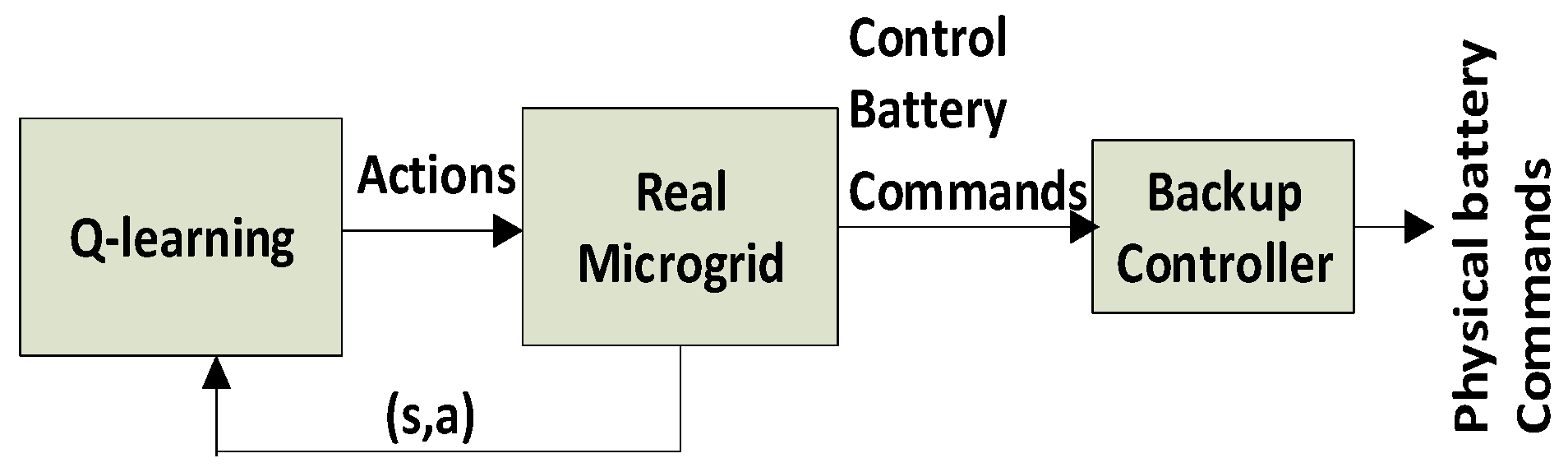
3.2. Online RL Implementation

Online RL is applied directly to real data in real time. Therefore, the agent learns the optimal policy by interacting with the real system. There is no pre-training in this online approach, unlike offline techniques. Figure 3 shows the online RL for EMS. The online RL algorithm updates the actions of the battery and dispatches them every 30 min in real time regardless of the status of convergence. Learning can be very slow, especially in first few days. Before convergence, the performance would be suboptimal. With time, the agent develops an optimal policy. The function of the backup controller in the online RL implementation is the same as for offline RL, as described in Section 2.3.

There is no separate training stage in online RL; rather, the agent gathers experiences during real-time interaction with the environment. Therefore, in the beginning, the Q-table is initialised with a shortsighted future reward with the algorithm hyper-parameter γ set to 0. Then, the table will be updated in real time by interacting with the real system. This simple initialisation step reduces the convergence time substantially as per [44].

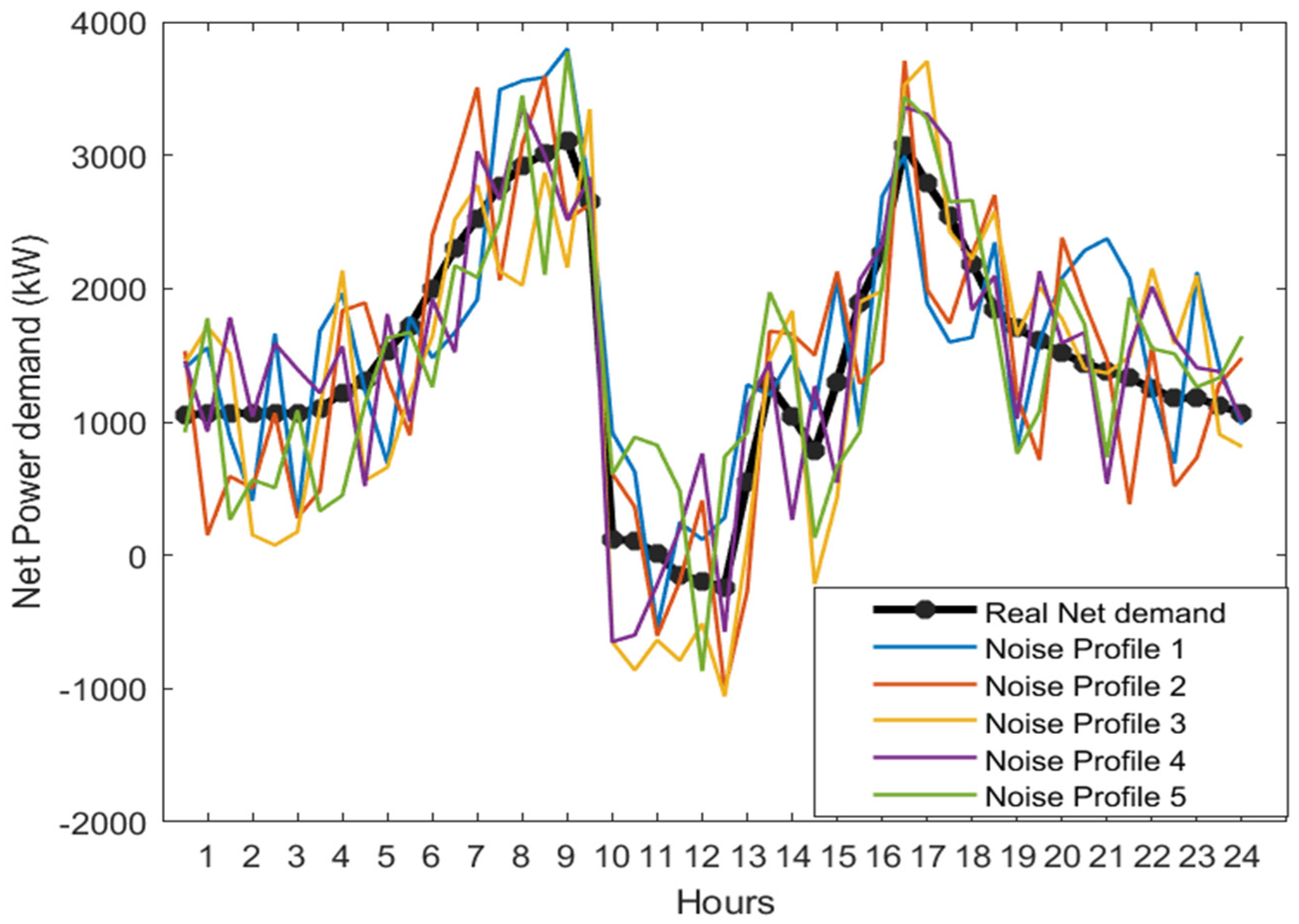
3.3. Prediction Error Generation

To compare the performance of both offline and online Q-learning, there is a need to create a difference between forecasted data (PV and load) and real data to represent the prediction error. We use an algorithm to add random noise to the real net power demand given by $e_t^{Net}=e_t^{demand}-e_t^{PV}$. The real PV and load profiles for a complete year are obtained from [45]. The noise is generated using normally distributed white Gaussian noise having different standard deviation (σ) values. For each σ, five noise profiles are generated, averaged, and then added to the real net power demand data to produce the forecasted net power demand, as shown in Figure 4. The increase in the σ value will increase the standard deviation error. Thus, the forecasted net demand with higher sigma values represents an increasing trend of deviation with respect to the real power demand and vice versa.

4. Simulation Results

This section evaluates the performance of the offline and online optimisation techniques. The offline and online RL were both applied on a daily basis with an interval of 30 min. Firstly, we compared the results of offline RL with MILP to analyse the efficiency of both algorithms in terms of cost saving in a grid-tied microgrid system. Then, we compared offline RL with online RL after establishing a benchmark between the offline RL and MILP techniques. In this regard, both the offline and online RL optimisation techniques need to be investigated in terms of cost saving per year. This work compares the behaviour of both the approaches when there is a different percentage of errors present between forecasted and real data profiles (PV and load). This information can be used to decide between offline and online RL when the real data (PV and Load) profiles deviate from the forecasted data. The real data assumed in this work are gathered from the online open-source data platform in reference [45]. The chosen parameters used to simulate the behaviour of the microgrid are provided in Table 1.

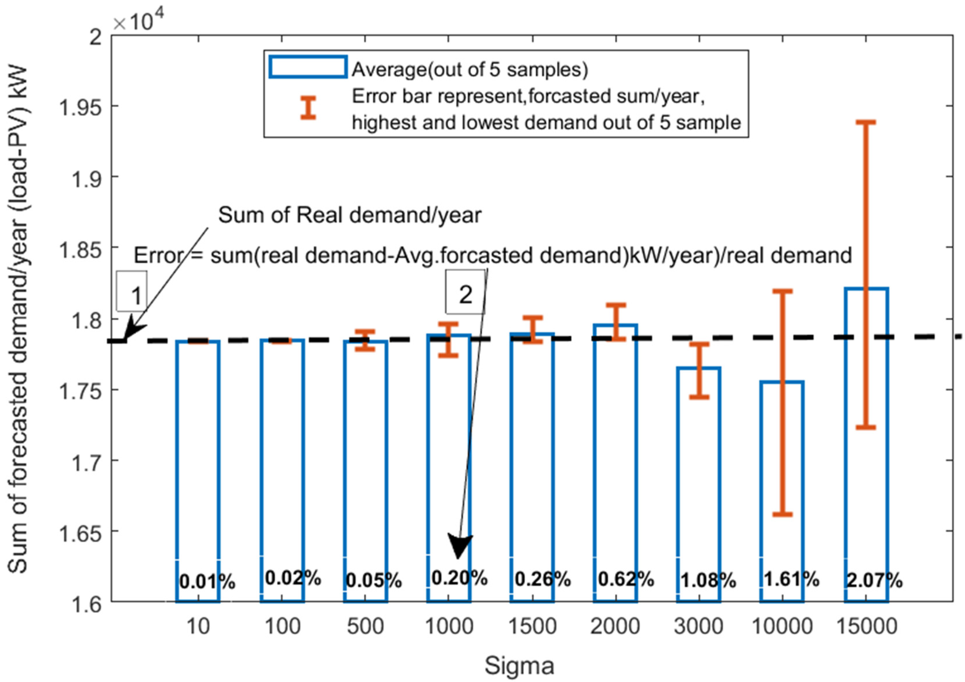
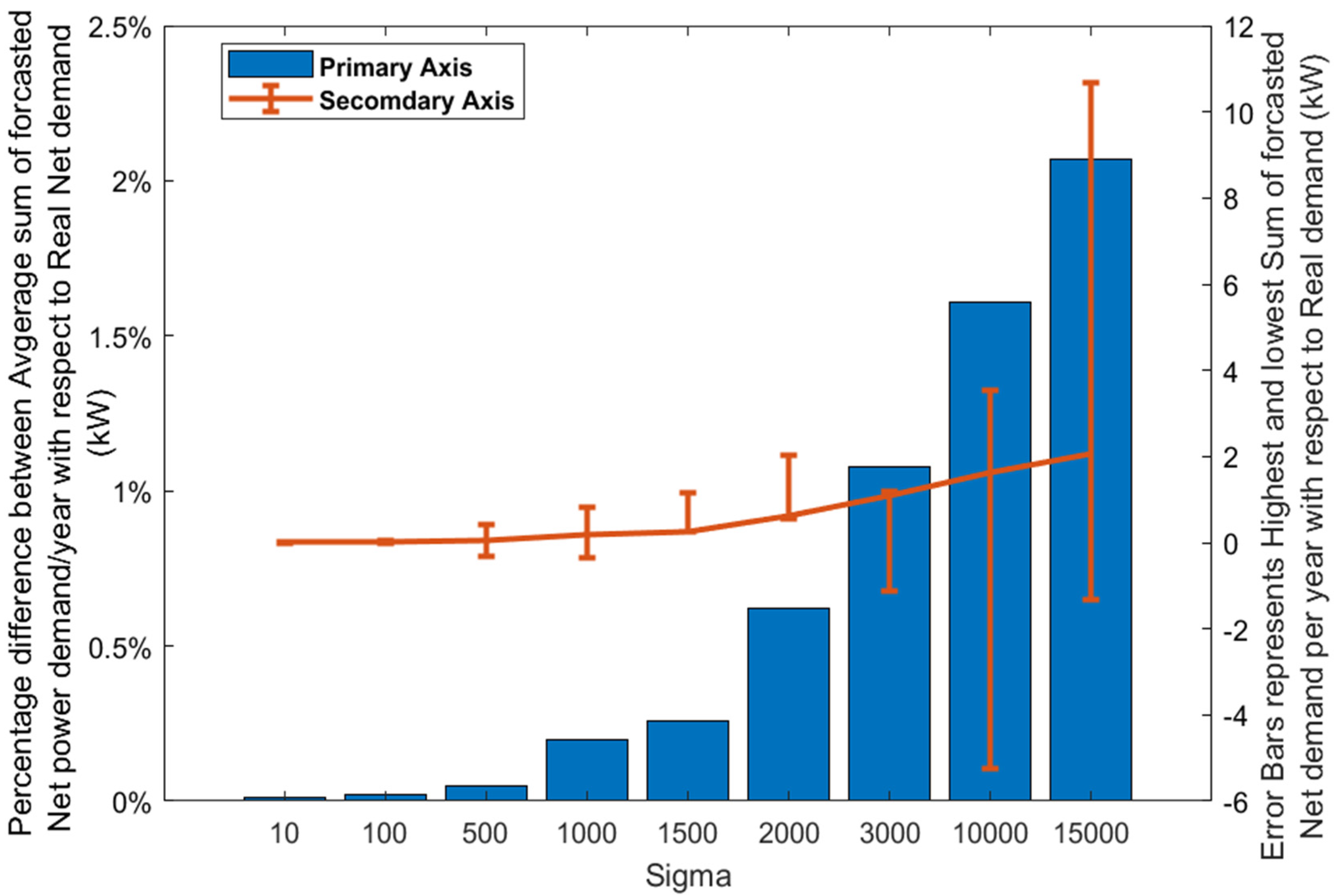
Below, Figure 5 shows the average net forecasted $e_{forecast}^{sum/year}/5$ demand per year using all five samples at each σ. Then, Equation (12) is used to find the percentage error between the real and forecasted power demand per year:

$$Ne{t}^{error/year}=\frac{1}{n}{\displaystyle \sum _1^n\left(\frac{e_{Real}^{sum/year}-e_{forecast}^{sum/year}}{e_{Real}^{sum/year}}\right)}.$$

(12)

The error bars in Figure 5 above show the $Ne{t}^{error/year}$ for each sigma using the highest and lowest sample of $e_{forecast}^{sum/year}$. The arrows indicating 1 and 2 in Figure 5 indicate the constant $e_{real}^{sum/year}$ and varying $Ne{t}^{error/year}$ in Equation (12), respectively.

Figure 6 depicts the difference between the generated $e_{forecast}^{sum/year}/5$ and the real power demand. The difference of the total real power demand per year with the highest and lowest sum of the generated forecasted power demand per year out of five samples at each sigma is described using the error bars on the secondary axis of Figure 6.

The two datasets, real (original) and forecasted (synthetic), are related to the net power demand per year and used to compare the performance of offline and online RL. Firstly, we compare offline MILP with offline RL by considering both the forecasted and real data profiles (PV, load demand) to be the same for both approaches. The results (Figure 7) show that both approaches have almost identical performance in terms of cost optimisation of the microgrid, with negligible difference. Over that small difference, MILP behaves slightly better due to the convergence requirements of RL. Therefore, the offline approaches, such as MILP and RL, which use the same forecasted and real data (having 0% error) for training, are equally good in real time.

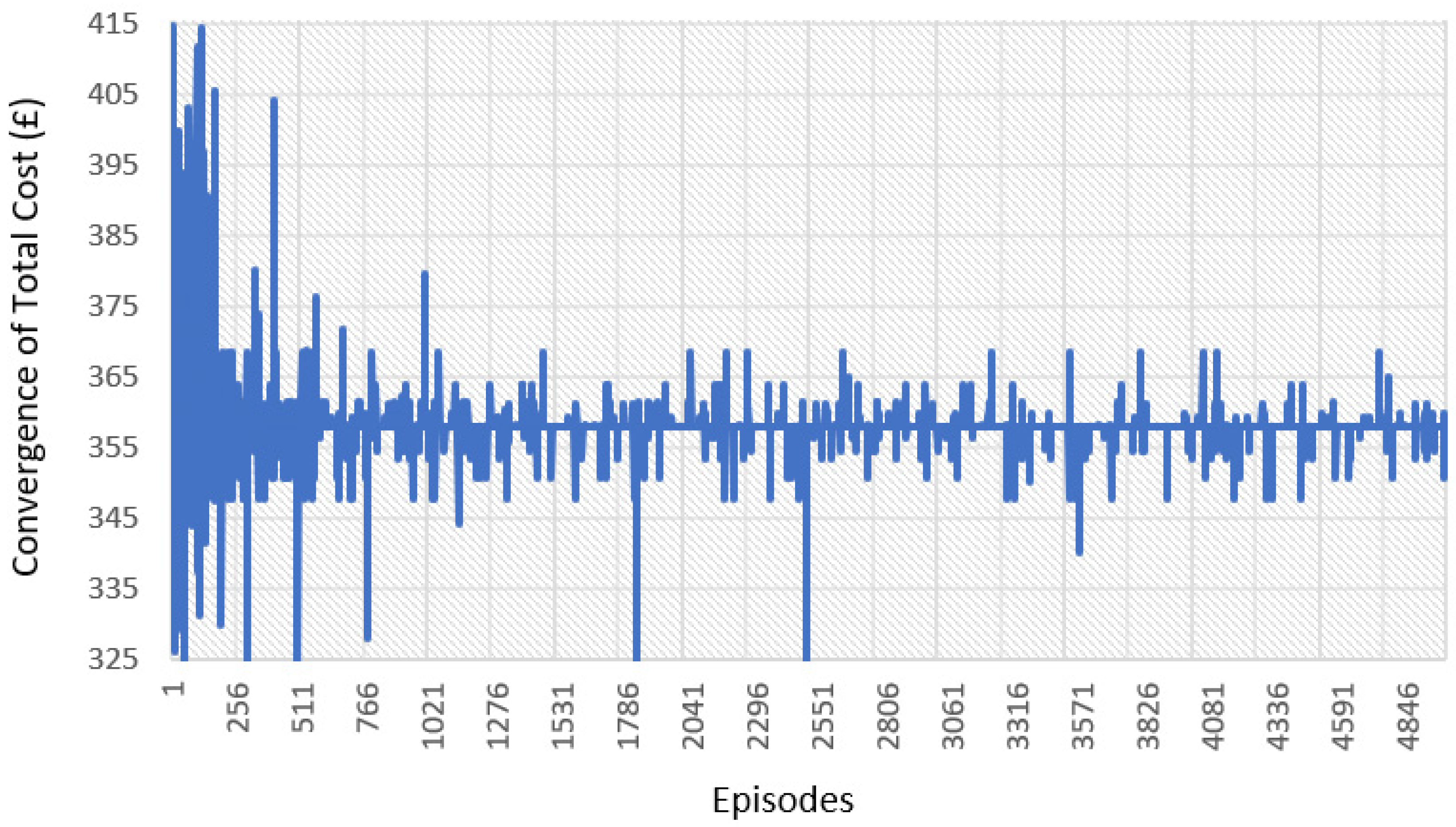
Figure 8 shows the convergence in terms of cost using offline RL. In this figure, only real data (PV and load) profiles were employed to analyse the convergence pattern of the offline RL as an ideal case. In the beginning, the cost is high and the curve shows random behaviour. As the number of episodes increases, the learning ability of the agent improves until the Q-table converges to show the optimal cost.

4.1. Offline vs. Online RL with No Forecast Error

The performance of the two RL approaches is first compared when there is no forecast error; i.e., the forecast data are the same as real data. Of course, this ideal situation does not exist in practice, but it provides an initial benchmark for the results. Both RL approaches are implemented as explained earlier in Section 3.1 and Section 3.2. In addition, MILP was also used to optimise the battery operation. 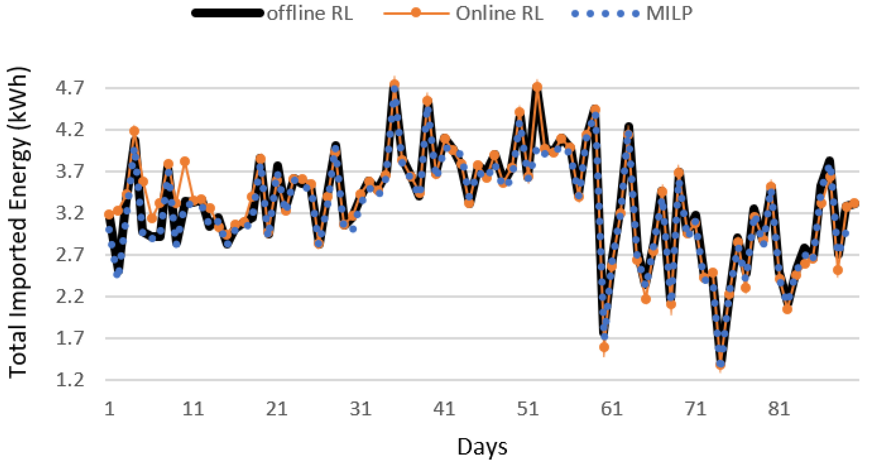Figure 9 and Figure 10 show the energy imported from the grid with respective cost on a daily basis, respectively. It can be seen that when the forecast error is zero, offline RL produces superior results. In Figure 9 and Figure 10, it can be seen that before the convergence of the online RL algorithm, a higher amount of grid energy is imported; therefore, the cost is also higher with respect to offline RL in the initial days. However, as the days progress and online RL learning converges to the optimal policy, the controller follows the same pattern as offline RL in terms of cost saving and reducing the imported energy. In this work, convergence was achieved in between 75 and 90 days in the case of online RL.

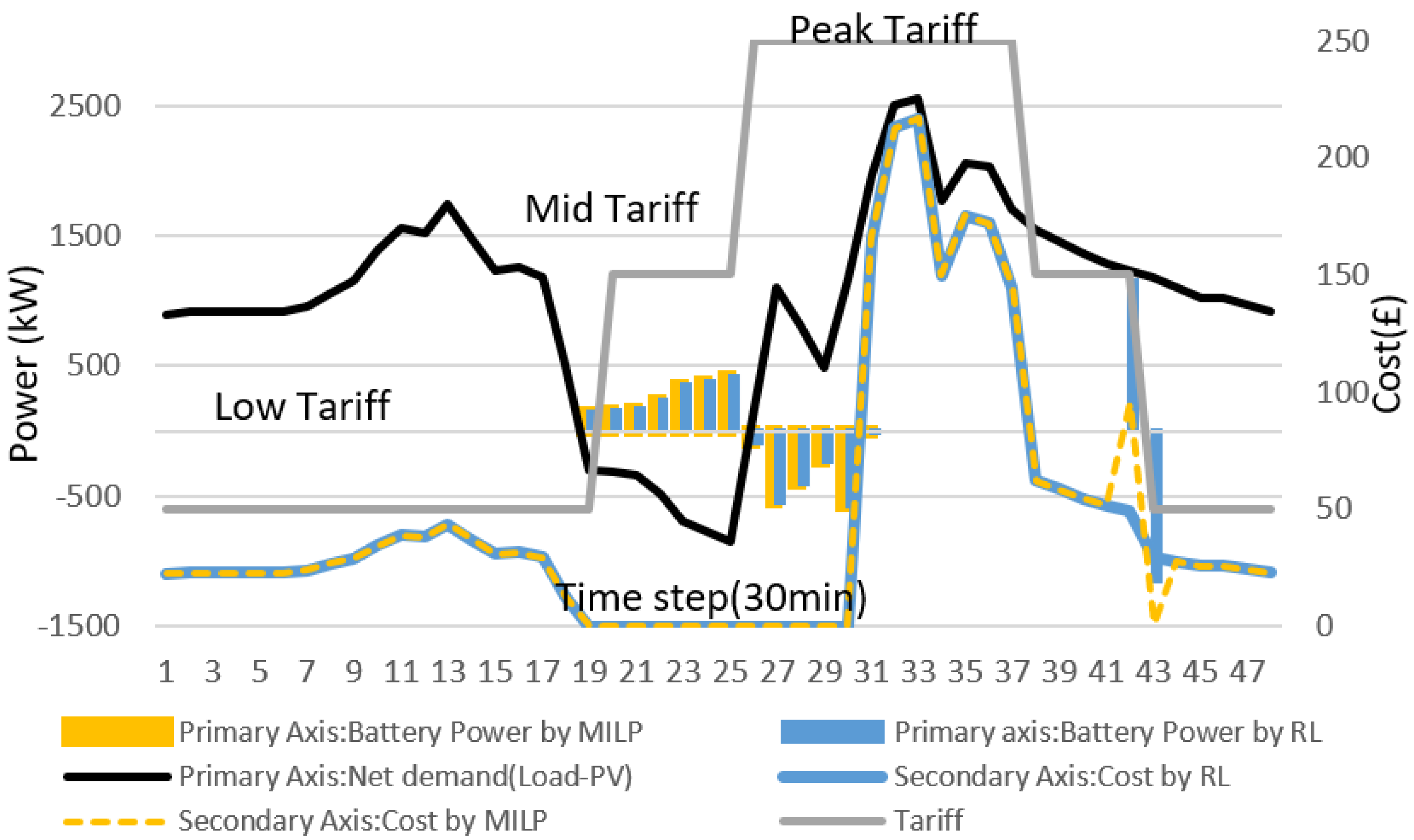
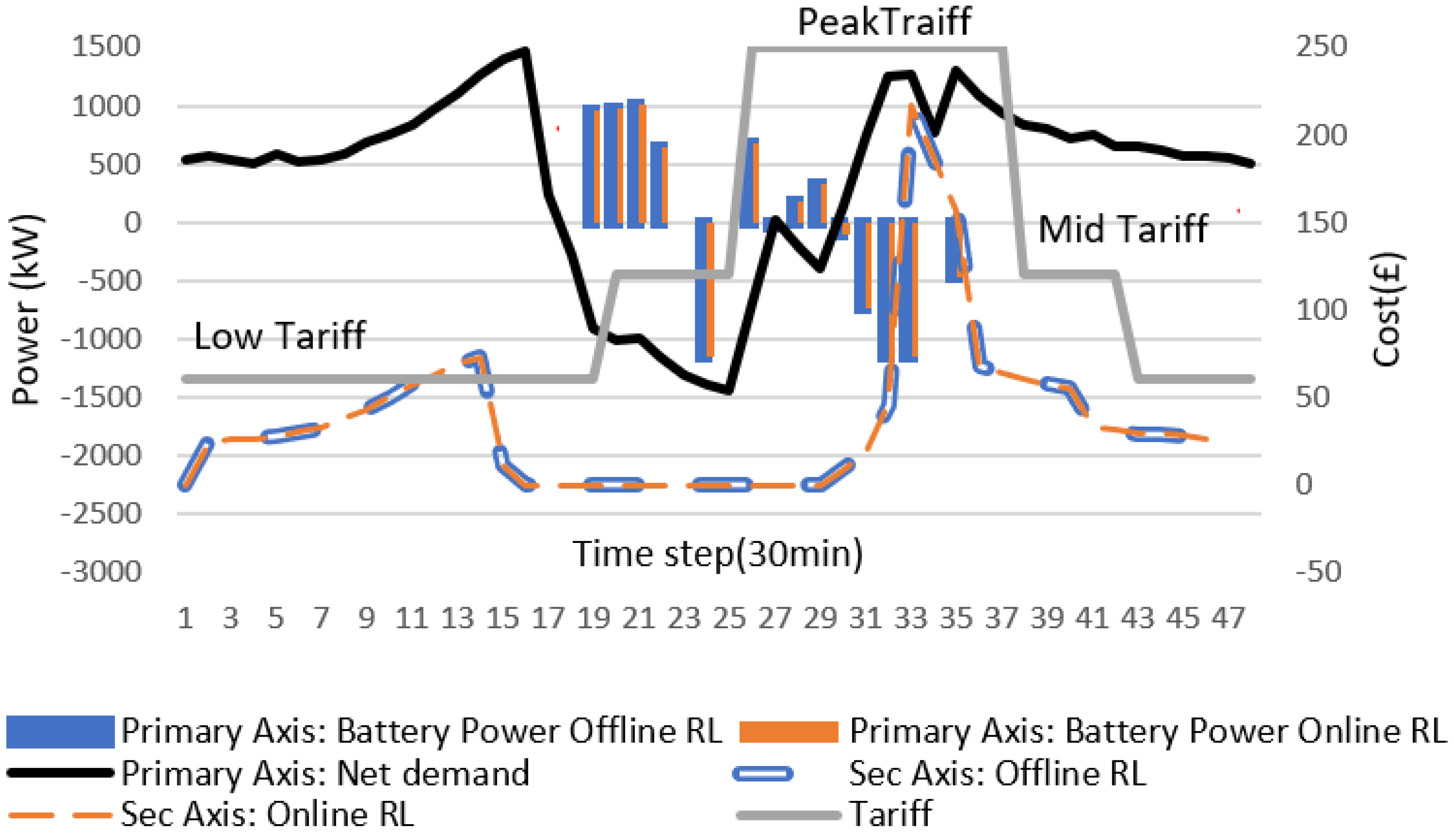
Figure 11 shows the overview of the battery actions generated in an average day after applying the Q-learning algorithm. We used the offline RL for a single day in Figure 11 to show the different states of the battery after convergence during different time intervals of the day with respect to load demand and PV availability. The difference between the load and PV ($e_t^{Net}$) is shown in the graph below at each time step. The $e_t^{Net}$ can be negative if the PV power generated is greater than the load demand at time t. The suggested battery actions by the RL agent pass through the backup controller to accommodate all physical constraints, as described in Section 2.3. As shown in Figure 11, when $e_t^{PV}>e_t^{Net}$ at time t, the battery charges from the current PV power up to the maximum level of ∆e after fulfilling the load demand. The outstanding PV power is sold to the main grid. During discharging, the battery discharges up to maximum level of ∆e either to fulfil the load demand or sell power to the utility grid.

Figure 11 is the randomly selected day of the year when both online and offline RL converge. The plot shows the same battery actions for both offline and online RL. Therefore, the cost achieved in both approaches are also same.

4.2. Offline vs. Online with Varying Forecast Error

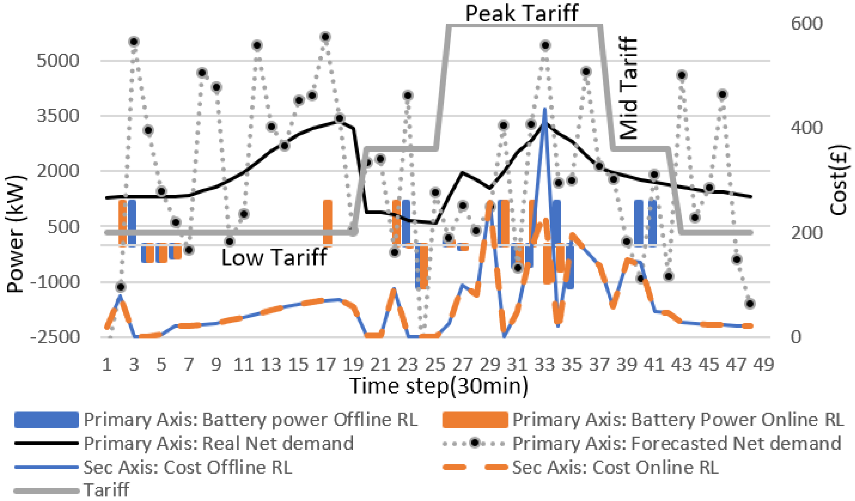
The forecasted profiles generated in Section 3.3 are used by the offline RL to create the battery charge/discharge/idle commands, which are then applied to the real data as was explained in Section 3.1 and Figure 2. For online RL, real data are used to generate the battery commands that are directly applied to the physical microgrid system. Figure 12 shows the overview of the battery actions (kW) generated in an average day after introducing 1.6% forecasted error with respect to the real net demand. Figure 12 also showed the daily cost of offline and online RL. The offline RL cost is higher than that of online RL at the time steps 31 to 35. Therefore, the overall average cost of offline RL in a day is higher than that of online RL (after convergence).

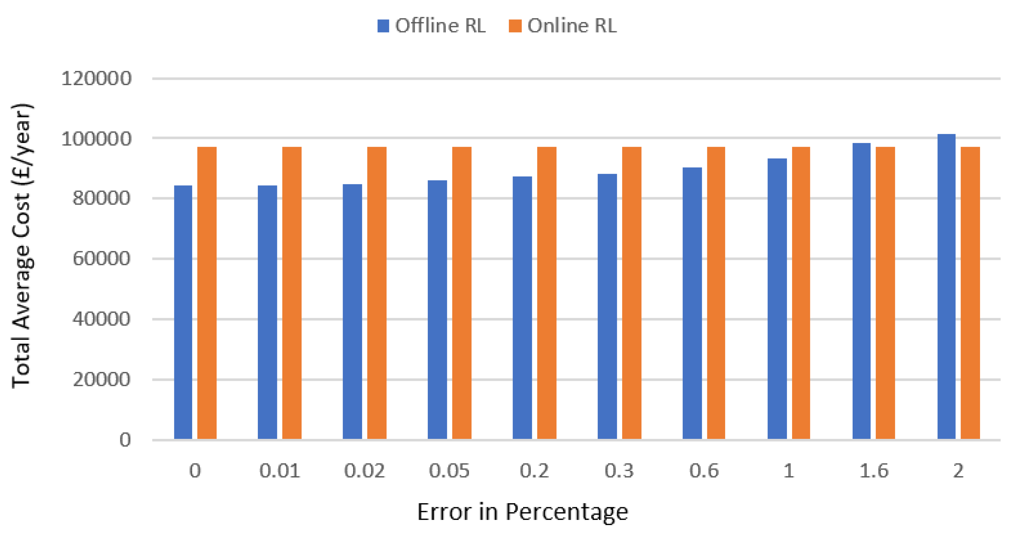
Figure 13 shows the optimal average cost achieved per year for both offline and online RL.

The results show that the average cost and imported energy of the offline Q-learning increase as the relative error between the forecasted and real power demand grows or vice versa. The error between real and synthetic predicted profiles are calculated using Equation (12). A rise in the value of the standard deviation reflects the increase in the error (in percent), as shown in Figure 5. Therefore, the noise level (σ) and the relative error are proportional to each other. At the start, when the error of the forecasted demand with respect to the real demand is low, the offline Q-learning performs better in comparison with the online RL in terms of cost optimisation per year. However, as the error increases, for example at 1.61% (between forecasted and real net demand), the online Q-learning begins to perform better and results in a lower cost than the offline Q-leaning.

5. Discussion

In this study, we report a comparison between the offline and online optimisation approaches to reduce the operational cost of a grid-connected microgrid by optimally managing the BESS in the presence of forecasting error. A variation between the forecasted and real-time demand may occur due to a change in the weather, ultimately affecting the suggested real-time optimal battery actions obtained through offline training. Hence, the results may not be optimal in terms of reducing cost. To avoid the complication of using forecasted data profiles (PV, load) offline, the literature suggested the online Q-learning [44]. However, online Q-learning needs some days to converge, as its training happens online after exploring real-time data. This knowledge gap in the existing research indicated a need for thorough analysis and comparison of both offline and online approaches. Therefore, we proposed the comparison between offline versus online algorithms on an annual basis. Conventional MILP and offline RL show approximately similar behaviour in terms of saving cost in microgrid operation. Then, the average annual costs of offline and online RL approaches were analysed using different forecasted data profiles. The synthetic forecasted data with respect to real data were produced by adding random white Gaussian noise with specified standard deviation.

Table 2. Proposed offline and online RL on the current application scenario.

Reference	Application	Used Method	Future Approach and Strategy
[3]	Sizing large-scale thermal energy storage (TES)	MILP	Apply offline day beforeApply online in real time
[4]	Minimise the use of fossil fuels	LP and MILP	Online RL
[7]	Reduce the cost	GAMSCPLEX	Online RL
[27]	Multi-objective Optimisation	MINLP guided by Q-learning	Multi-objective RL (online/offline)
[46]	Control load shedding	IOT, mathematical modelling	Online RL
[47]	Energy trading and security	Blockchain based	Compare block-chain based mechanism with RL (online/offline)
[48]	Power management	Fuzzy logic controller	Offline RL
This work	BESS management in MG	Offline and online RL	Apply offline RL for training, online RL at real time

suggested the possible implementation of offline or online RL on modern research to optimise the economy of power systems. For example, different type of optimisation problems were solved by using different methods in the past, as mentioned in Section 1. These solutions faced a range of challenges, including convergence, inefficient optimisation (cost, Co2 Emission), and computational time under different or varied conditions. The scope of this article suggests that reinforcement learning (offline/online) has full potential to deal with the different types of optimisation problems and challenges.

6. Conclusions

The following are the key findings of this paper:

• When the error is in between 0 and 1.5%, the offline RL algorithm performs better in terms of cost with respect to the online RL.
• In the first few days, RL performs better as it converges from day 1, while online RL shows better results in terms of cost after a few days. The number of days may vary depending upon the difference between the real and forecasted demand.
• The operating cost of the microgrid is proportional to the imported energy from the main grid by considering PV and battery operating cost equal to zero.
• The computational cost and time of offline RL is higher than that of online RL.
• In the literature [10,11,12,13,14,15,16,17,18], it was evident that the forecasting of PV has less accuracy than load forecasting.

Therefore, a higher difference between forecasted and real PV and load profiles suggests adopting an online Q-learning approach. For example, there are certain countries and areas where the forecasting of PV and load demand are not certain due to abrupt changes in the weather condition or the user behaviour. The actual energy demand at run times may change a lot in contrast to the predictions. The online Q-learning for cost optimisation provides a better solution in these regions. While operating in favourable prediction conditions, the offline Q-learning performs better.

In the future, there may be other quantification methods such as root mean square error (RMSE) that can be used to introduce errors in forecasted data with respect to real data to compare these two approaches for other type of noise distributions. In the future, both offline and online Q-learning approaches may be employed as a two-layer structure. This can provide a better and more efficient solution for the cost optimisation in a real microgrid.