Article

The Potential of Variable Renewable Energy Sources in Mexico: A Temporally Evaluated and Geospatially Constrained Techno-Economical Assessment

by
Edgar Ubaldo Peña Sánchez
1,*,
Severin David Ryberg
1,
Heidi Ursula Heinrichs
1,
Detlef Stolten
1,2 and
Martin Robinius
1
1
Institute of Energy and Climate Research—Techno-Economic Systems Analysis (IEK-3), Forschungszentrum Juelich GmbH, 52425 Juelich, Germany
2
Chair for Fuel Cells, Faculty of Mechanical Engineering, RWTH Aachen University, 52072 Aachen, Germany
*
Author to whom correspondence should be addressed.
Submission received: 7 July 2021 / Revised: 24 August 2021 / Accepted: 1 September 2021 / Published: 14 September 2021

Abstract

:
Due to the increasing global importance of decarbonizing human activities, especially the production of electricity, the optimal deployment of renewable energy technologies will play a crucial role in future energy systems. To accomplish this, particular attention must be accorded to the geospatial and temporal distribution of variable renewable energy sources (VRES), such as wind and solar radiation, in order to match electricity supply and demand. This study presents a techno-economical assessment of four energy technologies in the hypothetical context of Mexico in 2050, namely: onshore and offshore wind turbines and open-field and rooftop photovoltaics. A land eligibility analysis incorporating physical, environmental, and sociopolitical eligibility constraints and individual turbine and photovoltaic park simulations, drawing on 39 years of climate data, is performed for individual sites across the country in an effort to determine the installable potential and the associated levelized costs of electricity. The results reveal that up to 54 PWh of renewable electricity can be produced at a levelized cost of electricity of less than 70 EUR·MWh−1. Around 91% (49 PWh) of this electricity would originate from 23 TW of open-field photovoltaic parks that could occupy up to 578,000 km2 of eligible land across the country. The remaining 9% (4.8 PWh) could be produced by 1.9 TW of onshore wind installations allocated to approximately 68,500 km2 of eligible land that is almost fully adjacent to three mountainous zones. The combination of rooftop photovoltaic and offshore wind turbines accounts for a very small share of less than 0.03% of the overall techno-economical potential.

1. Introduction

The last decade has seen a significant increase in the contribution of renewable energy technologies to the reduction of anthropogenic CO2 emissions. Currently, renewables account for around 34% of global installed power capacity [1], and investments in them have grown steadily by at least 10% per year over the last decade [2], spurred by cost reductions and technological improvements [3]. Moreover, international commitments in the form of environmental policies and market integration mechanisms, such as those outlined in the 2015 Paris Climate Agreement [4], underpin the trend towards increasing renewable power generation. Hence, in order to aid policy initiatives and the other decision-making processes necessary for an effective energy transition, the generation potential of renewable energy technologies must be assessed with consideration given to their intrinsic geospatial and temporal heterogeneity for optimizing their use.

1.1. Mexico’s Profile

Mexico is currently an upper-middle-income country [5] with the world’s fifteenth-largest economy [6] and tenth-largest population [7]. Its economy is closely linked to that of the rest of the world as a member of the United Nations, the World Trade Organization, the G8 + 5, the G20, and as a signatory to the Paris agreement, among other connections. In terms of energy, Mexico has traditionally been a crude oil exporter with a fossil fuel-intensive economy [8]. Nonetheless, Mexico has experienced a continuous 15-year decline in crude oil production that has been offset by increasing refined oil products and natural gas imports in order to fuel the country’s transportation and power sectors [8]. In 2015, Mexico was responsible for the emission of 490 MtCO2-eq annually [9], making it the twelfth most polluting country worldwide, even surpassing some fully industrialized economies, such as those of France and the United Kingdom [10]. In 2017, the power sector satisfied 330 TWh of electricity demand, of which only 15% originated from renewable sources [11], making it the second most polluting sector after transportation [9]. Moreover, over the last 13 years, Mexico’s electricity consumption has steadily grown by 3% per year on average and is “directly” linked to the growth of gross domestic production [11].
For the coming years, Mexico not only has increasing green commitments to implement but also remaining energy challenges that should not be met at the expense of damaging the environment. For instance, it must provide reliable electricity access to an estimated 3.5 million people in remote areas [12] while at the same time reducing its total greenhouse gas emissions by 22% before 2030 [9]. Moreover, by 2050, Mexico’s population is expected to reach over 155 million (nearly 25% more people than in 2020) [13], and its economy could become the world’s sixth largest [14]. Thus, Mexico’s energy needs will be even larger and more complex than those of today. Therefore, the development of its energy sector requires the integration of all renewable energy sources. Fortunately, apart from traditional renewable sources such as hydropower, geothermal, and bioenergy, Mexico enjoys abundant sunshine across the country and regional strong winds that must be techno-economically assessed in order to optimize their use.

1.2. Literature Review

Past studies have employed a mixture of methodologies and generally lack the comparable and reproducible models and data inputs that are necessary to assess renewable energy in Mexico, which hinder a direct comparison between assessments. In 1995, the first national onshore wind assessment was conducted by Schwartz et al. [15], in which regional wind zones with both high and poor potentials were identified and formed the basis of most of the subsequent regional wind energy assessments. For instance, Jaramillo et al. [16] concluded that in the federal state of Baja California, a region with high wind potential identified by Schwartz et al., the average levelized cost of electricity (LCOE) from onshore wind would be around 50 EUR·MWh−1. Later, in 2010, Hernández Escobedo et al. [17] assessed the wind potential of the entire country, estimating that a modeled 750 kW turbine could operate with 1700 full load hours (FLH) on average. However, the corresponding LCOE was not provided, and the model used was not open source, which makes the findings difficult to compare. Subsequently, Hernández Escobedo et al. [18] performed a similar analysis with a 1.5 MW wind turbine in the state of Veracruz. The result was an FLH estimation of around 1750–2630 h per year. This second study did not include an LCOE estimation either. Likewise, the works of Figueroa Espinoza et al. [19], Carrasco Diaz et al. [20], Carreon Sierra et al. [21], and Hernández Escobedo [22] focused on different regions in Mexico but again did not include detailed techno-economical parameters in their results. In 2019, Rodriguez Hernández et al. [23] employed yet another methodology to assess the economic feasibility of small wind turbine designs in the Mexico City region and reported that only turbines with capacities of 0.5 and 0.8 kW, which are not in line with recent and future trends in utility-scale onshore wind turbines [24], could be economically viable in the region.
Most assessments hitherto have only focused on onshore wind potential and, to the authors’ knowledge, only one study, the “National inventory of zones with high potential for clean energy” (AZEL) [25], estimates open-field photovoltaics (PV) potential nationwide. Furthermore, again to the best of the authors’ knowledge, offshore wind energy and rooftop PV have not yet been assessed on a national level. The AZEL assessment carried out by the National Ministry of Energy (SENER) consists of estimations of renewable energy potentials based on an energy density analysis presented via a geographic information system (GIS) map of onshore wind and open-field solar PV, among others. Although the AZEL report is the first assessment to offer some land exclusion constraints for the placement of PV parks and onshore turbines, such as protected areas, human settlements, transportation roads, transmission lines, minimum continuous areas (ignores the sparse land available for installations smaller than up to 12.5 km2), terrain elevation, airports, coastal lines, and minimum wind speed, it does not provide techno-economical details on the costs of electricity production. The AZEL report also fails to provide time series generation profiles, account for efficiency gains over time due to technology advancement, and offer the optimal arrangement of VRES installations or the cost functions that are necessary to more precisely estimate green potential.
Internationally, relevant renewable energy assessments have incorporated complementary considerations and progressively improved their accuracy and standardization. McKenna et al. [26] modeled onshore wind potential for Germany using wind speed data with 1 km2 spatial resolution, multiple wind turbine designs, and a detailed land eligibility analysis (LEA). Building on McKenna’s approach, Jäger et al. [27] assessed the onshore wind potential of Baden-Württemberg, Germany, positioning wind turbines according to the wind direction to maximize the utilization of the available land and accounting for wind blocking from neighboring turbines. Staffell and Pfenninger [28] used NASA’s MERRA-2 database [29] over 20 years to re-analyze previous wind power assessments and found that, depending on the weather of a particular year, wind assessments could differ by up to 50% in terms of capacity factors and total generation output. The researchers concluded that taking larger weather timespans could help reducing weather variability across different years. Robinius et al. [30,31] also applied LEA and turbine positioning algorithms in a wind assessment for Germany for an advanced onshore wind turbine as part of a 2050 energy system simulation of Germany. Later, Ryberg et al. [24,32] assessed the onshore wind, open-field PV, and rooftop PV potential in Europe to investigate the occurrence of lulls in electricity production, incorporating and improving upon the cumulative progress of past approaches. Ryberg’s study included an extended LEA [33,34] and the modeling of futuristic onshore wind turbines [24] and advanced PV panels to account for technological progress in the foreseeable future [24], as well as a scalable VRES placement algorithm and a quasi-physics-based algorithm to calculate the generation profiles and apply some air density and sunlight irradiation corrections. Finally, Caglayan et al. [35] adopted Ryberg’s methodology to calculate the potential of offshore wind energy for Europe, also adding the investment cost estimation function described by Fingersh et al. [36] and Maness et al. [37] as a function of the foundation type, distance to shore, and ocean depth.

1.3. Contribution of the Paper

Due to the recent progress in the field not being applied to Mexico and given the large methodological divergences in previous assessments, this study aims to assess the techno-economical potential in the entire Mexican territory (Approximately 2 million km2 of land and 3.2 million km2 of sea (assigned to the nearest state)) of four VRES technologies: onshore wind, offshore wind, open-field PV, and rooftop PV for the future 2050 context using a state-of-the-art approach with tailor-made geospatial considerations. The ultimate objective of this work is that the results of this assessment to provide practical information to facilitate decision making for key stakeholders with respect to where renewable energy can be optimally exploited. The results can also serve as inputs for an optimal and sustainable energy system design at a national level.

1.4. Organization of the Paper

The study is structured as follows: Section 1 serves to introduce the relevance of the topic and to declare the main contribution of the paper. Next, the methodology is described in Section 2. The results and discussion are presented in Section 3 and Section 4, respectively. Finally, relevant conclusions are presented in Section 5.

2. Methodology

The selected assessment approach comprised three main steps. First, an extensive LEA was applied to Mexico, maintaining a particular emphasis on country-specific factors. The total eligible area per technology and distribution were obtained here. Secondly, the maximum number of VRES installments with their techno-economic parameters were individually derived by applying technology design correlations according to the local terrain and weather characteristics, as well as costing algorithms as utilized in the selected literature. Finally, quasi-physics-based renewable energy production simulations were carried out to obtain time series generation profiles for each installment. The average electricity generation, FLH, and LCOE were also calculated, and the VRES techno-economic potential was obtained by curtailing electricity production with an LCOE over 70 EUR·MWh−1 that corresponds to historic average electricity costs in Mexico according to data reported by the National Electricity Control Authority [38]. A more detailed description of the three main steps in the methodology is presented in the subsequent subchapters. The results, discussion, and conclusions are structured in accordance with the administrative state division, as well as geographical zones (shown in Figure 1) to help the reader follow the comparisons more easily.

2.1. Land Eligibility Analysis

The Geospatial Land Availability for Energy System (GLAES) model [39] developed by Ryberg et al. [34] was employed to determine the geospatially constrained eligible land for the investigated VRES technologies. In total, 34 land constraints and their technology-specific exclusion zones were considered. This large number of constraints was intended to underpin a conservative approach and avoid “environmental problem shifting” [40]. Table A1 in the Appendix A lists the land constraints and exclusion zones in detail for onshore wind, offshore wind, and open-field PV. The LEA for rooftop PV was only constrained by human settlements (house rooftops) in accordance with Ryberg’s approach [32]. For each technology, the spatial reference system EPGS 6263 [41] was used with a spatial resolution of 100 m2, as it represents a good trade-off between spatial fidelity, data availability, and computational intensity.
Of a total of 34 constraints, 27 were previously employed by either Ryberg et al. [32], Caglayan et al. [35], or Heuser et al. [42] and were kept unchanged because they do not conflict with the particularities of the Mexican context. Official datasets published by Mexican authorities were preferred when possible, as detailed in Table A1 in the Appendix A. Detailed justifications for the selection of these constraints, filtering procedures, and the buffer zones used can be found in the preceding works of Ryberg et al. [32], Caglayan et al. [35], and Heuser et al. [42], whereas the following subchapter describes in more detail the adjusted and additional considerations for the Mexican context.

Specific LEA Constraints for Mexico

Seven primary constraints specific to the context of Mexico are taken into account, which constitute the novel contributions of this work, namely: military areas, harbors, LNG terminals, geothermal sites, primary jungles, active volcanoes, and hurricanes. The reasons for their inclusion and the corresponding buffer zones assumed are also outlined. Details on the data sources and assumed buffer distances are included in Table A1 in the Appendix A. In general, international data sources were used, following Ryberg et al.’s [43] methodology for the most part. Nevertheless, data from national sources were preferred with respect to constraints relating to demographics, energy infrastructure, and land use, as they were generally more up to date than international data sources.
All VRES placements within 1 km distance from military areas, harbors, and LNG terminals were excluded due to the security issues entailed and the assumption that significant interference between VRES production and the operations conducted in these areas could occur. In a 200 m radius from geothermal sites, where geothermal energy systems can potentially be installed, placements were restricted to maintain the potential of this renewable energy source. Placements in primary jungles and within 1 km of their surrounding areas were excluded to protect biodiversity, as recommended by the SENER’s environmental evaluation [44]. Based on the conclusions of Capra et al. [45], circular exclusion areas with a radius of 2 km from active volcanoes’ vents were excluded for onshore wind turbines and open-field PV parks to avoid the risks related to volcanic activity. Offshore wind turbines were considered by the authors not to be subject to these risks, as they must be placed in water at least 15 km from coastlines [35], and no records of marine volcanic eruptions in those areas of Mexico could be found. Similarly, areas hit by hurricanes of category 3 or above, as per data from 1980 to 2019 by the US National Oceanic and Atmospheric Administration (NOOA) [43], were excluded for both wind turbine installation variants. Category 3 hurricanes have a maximum sustained wind speed above 60 m/s, in accordance with the limit of most commercial wind turbines’ resistance (40–80 m/s) [46]. The exclusion zone, in this case, is taken as 30 km, as this is the maximum radius at which any hurricane has shown sustainable wind speeds above 60 m/s [47]. This security buffer is increased to 50 km for PV installations where not only wind speeds but also flying objects can cause damage.
Land constraints such as radio towers, land instability (i.e., the likelihood of landslides), and ground composition considered by previous authors [48,49,50] were not included herein due to a lack of these data existing for Mexico. A minimum distance to a transmission line is not considered applicable in the case of Mexico in 2050, as the country’s electricity demand is expected to grow considerably [11], adding the need for extensive grid expansion and, therefore, making the current status quo of connection not applicable to a 2050 context. Arguably, other LEA constraints such as earthquakes and tsunamis can potentially be included in an LEA for a country such as Mexico. Nevertheless, this study does not include these due to empirical evidence found in the literature presented in the Appendix A.

2.2. Techno-Economic Parameters

Once the available areas were obtained, GLAES was again used to place minimally separated elliptical or polygonal geometries representing either single turbines or solar PV parks, respectively. Around 1.6 million elliptical shapes representing onshore turbine rotors of 136 m in diameter oriented towards the 39-years average wind direction were incorporated in the available land with an inter-turbine separation of 8 × 4 times the rotor diameter (transversal x longitudinal axis) in accordance with Ryberg et al. [24]. Similarly, nearly 600,000 offshore turbines were modeled with a fixed rotor diameter of 210 m and separated by 10 × 4 times the rotor diameter, as per Caglayan et al. [35]. For PV technologies, polygonal shapes representing about 660,000 PV farms with several PV strings and 20 km2 of PV-covered house roofs were assigned following Ryberg’s [32] approach. Next, the technology’s design parameters were obtained. Futuristic onshore wind turbine design incorporated in the Renewable Energy Simulation toolkit (RESKit) [51] model for Python by Ryberg et al. [24] for a 2050 context were used to account for technological development. Utilizing this algorithm, design parameters such as hub height and specific capacity were inferred for each turbine from local wind speed and terrain characteristics for a given rotor diameter. When applied to the previously obtained placements, onshore turbine designs resulted in nominal capacities and hub heights ranging from 3.2 to 5.9 MW and 88 to 185 m, respectively. Individual onshore turbines’ total capital costs (CAPEX), ranging from 1090 to 1350 EUR·kW−1, were obtained according to the costing procedure used by the same author. A future 1100 EUR·kW−1 baseline cost design was assumed and assumed to cover the cost of capital, balancing of the system, and financial costs according to their CAPEX shares, suggested by NREL’s turbine cost breakdown [52] and costing relationships noted by Fingersh et al. [36] and Maples et al. [53].
With respect to offshore wind, a fixed turbine design with a hub height of 135 m, rotor diameter of 210 m, and capacity of 9.4 MW was selected following the approach of Caglayan et al. [35]. The only design parameter used to select offshore turbines was the foundation type that yielded the lowest LCOE of the four investigated options, i.e., monopole, jacket, semisubmersible, and floating spar according to the placement criteria used by Maness et al. [37]. Similar to their onshore counterparts, the CAPEX cost function of offshore turbines uses a 2300 EUR·kW−1 baseline design, resulting in a range of 1570–10,000 EUR·kW−1 due to cost additions arising from foundation type, sea floor depth, and distance to shore [35].
For PV technologies, the models Winaico WSx-240P6 (fixed tilt) for open-field and LG 360Q1C-A5 for rooftops were selected, in accordance with Ryberg’s methodology [32]. The tilt and azimuth angles were obtained on the basis of the Global Solar Atlas (GSA) [54] database for each PV park location, whereas the CAPEX assumptions correspond to 2050 projections by the Fraunhofer Institute [55] of 500 EUR·kW−1 for open-field PV and 800 EUR·kW−1 for rooftop PV modules. As in the case of wind turbines, the PV CAPEX is assumed to cover all costs associated with the installation. Furthermore, the technical parameters of the PV models were derived from the Go Solar California database [56], with a projected module efficiency of 24% and 30% for open-field and rooftop PV, respectively, as per the conservative projection for 2050 in the same Fraunhofer report.
The technologies’ annual operational costs (OPEX), as percentages of the PV CAPEX, and economic service lives were kept the same as the ones suggested by the corresponding costing methodology. The weighted average cost of capital (WACC) was fixed at 8% for all technologies to maintain consistency with similar assessments [24,32,42,57]. Regional differences in technology costs and access were not considered in the costing procedure. Nevertheless, the technology costs cited here are around 20% higher than those utilized by Sarmiento [58] for Mexico in the same 2050 context and, hence, represent a conservative approach. Table 1 summarizes the VRES techno-economic parameters utilized.

2.3. VRES Simulations and Techno-Economic Potential

The computational quasi-physics-based model Renewable Energy Source toolkit (RESKit) [51] was employed to simulate VRES production according to localized climate inputs and geospatial characteristics, as per the methodology of Ryberg et al. [24] for onshore wind and PV potentials. The methodology of Caglayan et al. [35], which also uses the RESKit model, was followed for offshore wind energy. A general description of the simulation procedure is offered here, but the reader is highly encouraged to refer to the original sources for more detailed information on the mathematical and physical foundations.
For onshore and offshore wind simulations, 39 years of available MERRA-2 weather data (1980–2019) from NASA [29] was processed to obtain long-term 50 m-height wind speed values at a 50 km2 spatial resolution. Onshore turbines were then adjusted to local contexts by using the global wind atlas (GWA) [59] to further improve the spatial resolution to 1 km2. Then, local wind speeds were projected to the turbines’ hub height using the roughness length factors estimated by Silva et al. [60] for the terrain type specified in the Corina Land Cover (CLC) dataset [61]. Offshore wind simulations utilize a constant 0.0002 m roughness lengths factor with bilinear interpolation, according to Caglayan et al. [35]. Subsequently, ideal gas air density was adjusted at the hub height by extracting the surface pressure and air temperature values from the MERRA-2 dataset, as suggested in IEC 61400-12 [62]. Finally, to account for stochastic wind energy losses, local wind speed values at the hub height were convoluted into synthetic power curves that were derived for each turbine as a function of its specific power. In this manner, the corresponding capacity factor at each hour in the weather data was obtained. The total annual generation and FLH were obtained by applying the simulations across the 39 years of data. The mean annual production and LCOE obtained represent historical averages over the evaluated time period.
For PV simulations, RESKit utilizes the already defined PV system location, module characteristics, and tilt and azimuth angles alongside weather data parameters such as air and dew point temperature near the surface, surface pressure, and near-surface wind speed. The model then outputs the capacity factors at each time step as a result of a multi-step process. First, the solar position is computed for each time step at each location using the NREL Solar Position Algorithm [63], for which the terrain elevation is obtained from the Global Multi-resolution Terrain Elevation Data [64] and pressure and temperature values from MERRA-2 are required. Then, extraterrestrial irradiance, relative air mass, and global horizontal irradiance (GHI) values at each time step were estimated as proposed by Spencer [65], Kasten and Young [66], and Perez et al. [67], respectively. Next, due to the low spatial resolution of the MERRA-2 dataset, the adjustment procedure used for the wind simulations was applied using the global solar atlas (GSA) [54] to the obtained GHI values. Subsequently, the plane of array (POA) as a sum of its components’ contributions (beam, ground reflected, and sky-diffuse) was computed in accordance with the methodology of Myers [68] and Perez et al. [69,70] and modified according to their respective angles of incidence according to De Soto [71] and Brandemuehl and Beckman [72]. Next, the cell temperature of the module was determined considering POA irradiance, wind speed, and air temperature with the method outlined by King et al. [73]. Afterwards, the DC electricity generation time series by the module was estimated as per the Single Diode model [71]. Finally, an 18% holistic loss was applied to account for inversion, wiring, soiling, and other losses according to values reported in the literature [54,74]. For more information about the PV simulation procedure, the reader is encouraged to refer to the original source [32].
Like any other resource, VRES generation potential is constrained by technological development (technical potential) but also by its cost of production (economic potential) [75]. Based on the relationship between VRES market value (refers to the amount of money that electricity generators can sell their electricity for in the wholesale electricity market without subsidies [76]) and historical electricity prices (refers to the time-weighted average wholesale electricity price [76]) proposed by Hirt [76], an LCOE threshold of 70 EUR·MWh−1 based on past electricity prices in Mexico [38] was applied to distinguish techno-economic VRES potential. The logic behind this assumption was that electricity production with costs higher than the electricity price would not be economically viable. The authors are of the view that comparing the electricity price to the LCOE is adequate as an initial approach to determining economic VRES potential.

3. Results

The results are grouped by their renewable source and are presented in the following subchapters. In the first place, the available area resulting from the LEA is expressed as a percentage of available land. Afterwards, the VRES simulations are presented using potential maps, graphs, and tables.

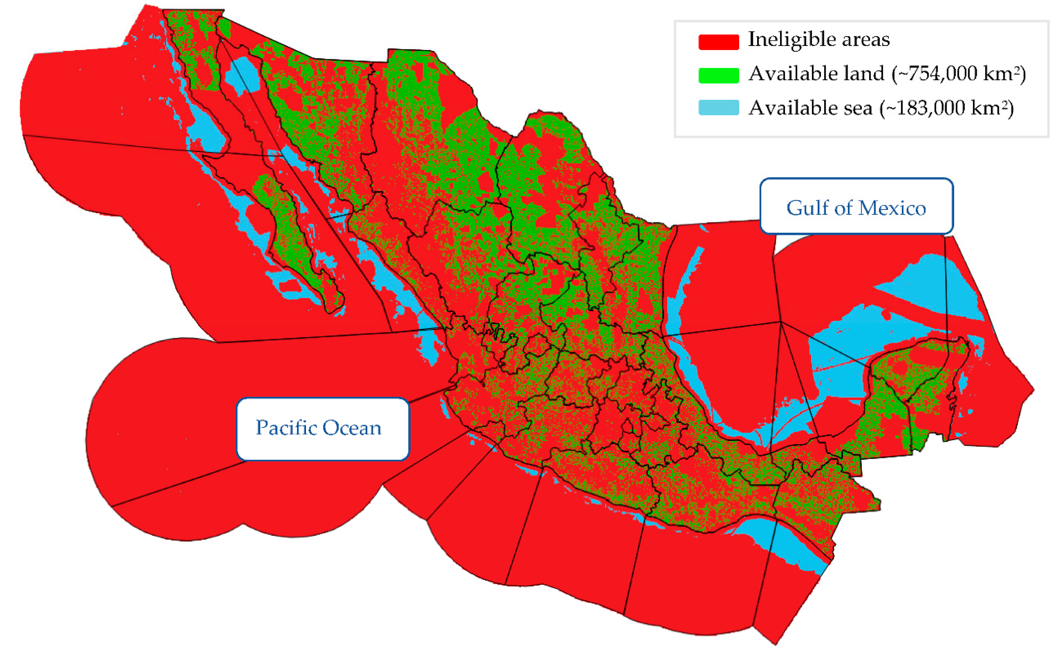
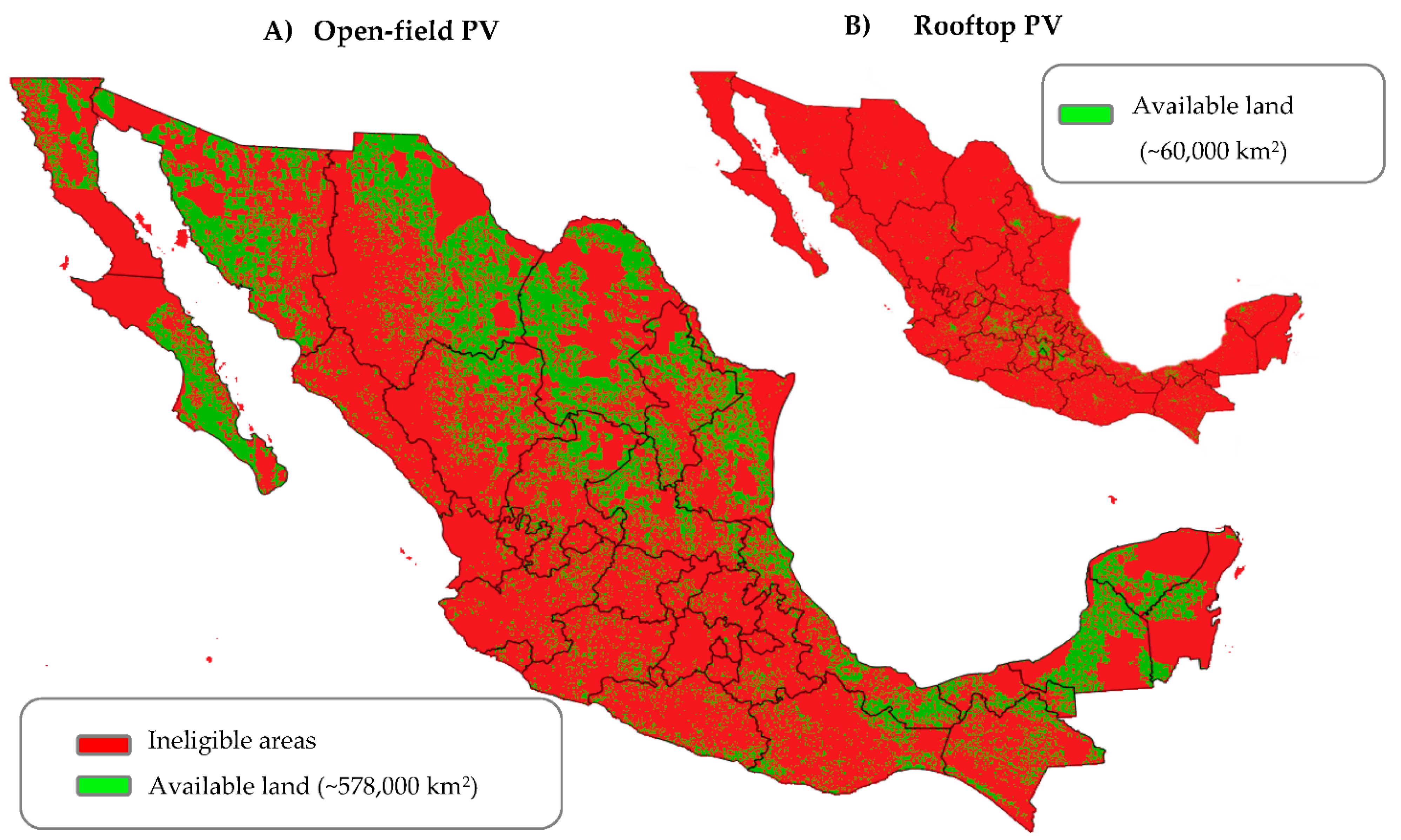
3.1. Land Availability

Figure 2 displays the area eligible for the placement of wind turbines. Around 754,000 km2 of land (~39% of the total) is eligible for onshore installations. Most of it is in the country’s northern states, where there are vast areas of uninhabited land and, to a lesser extent, in the southeastern states. The center of the country appears to have the least area eligible due to settlement-related constraints such as human habitation areas and roads. For offshore installations, a total area of around 183,000 km2 (~6% of the territorial sea) was found to be eligible.
By comparison, the eligible area for offshore turbines is four times less than that for onshore ones. Most of this is allocated along the Gulf of Mexico and Yucatan peninsula, where shallow waters qualify as eligible despite being affected by hurricane-prone and conservation constraints. The Pacific coast features little eligible sea area due to the local arrangement of the tectonic plates that results in abrupt ocean depth drop-offs. The western side of the Baja California peninsula and the Isthmus coast partially escape this effect, as they do not lie along the inter-tectonic line.
Figure 3 displays two maps corresponding to the land eligible for the placement of PV technologies: (A) for open-field PV; and (B) for rooftop PV. Open-field PV parks account for a total area of around 578,000 km2 (~30% of the territorial extension), which is around one-quarter smaller than the eligible area for onshore wind. There are three main reasons for this. The first is that, given the mountainous geography of Mexico, tougher slope-related constraints (with a maximum inclination of 17° for wind compared to 3° for PV) have a greater impact on the available land. Second, the exclusion zone for hurricane areas is larger compared to that for wind turbines, which considerably reduces the eligible area in the Yucatan peninsula. Third, agricultural areas, which account for around 17% of the total territorial land, are excluded for PV installations but not for wind. The total eligible rooftop area is around 60,000 km2 and has a distribution focused in major urban areas across the country, especially in the central region.

3.2. VRES Techno-Economic Generation Potential

The overall annual techno-economic VRES generation potential of Mexico was found to be 54 PWh. Of this, 49.2 PWh derives from open-field PV (91%) and 4.8 PWh from onshore wind (9%). Offshore wind (38 TWh) and rooftop PV (1 TWh) generation represent less than 0.03% of the combined total. Despite having the largest available land share, the wind resources in Mexico are regionally concentrated and less favorable by comparison to the solar ones. Larger eligible onshore wind areas do not translate into higher generation potential. The following subchapters present the wind and PV potential distribution across the country, subdivided into the zones presented in Figure 1.

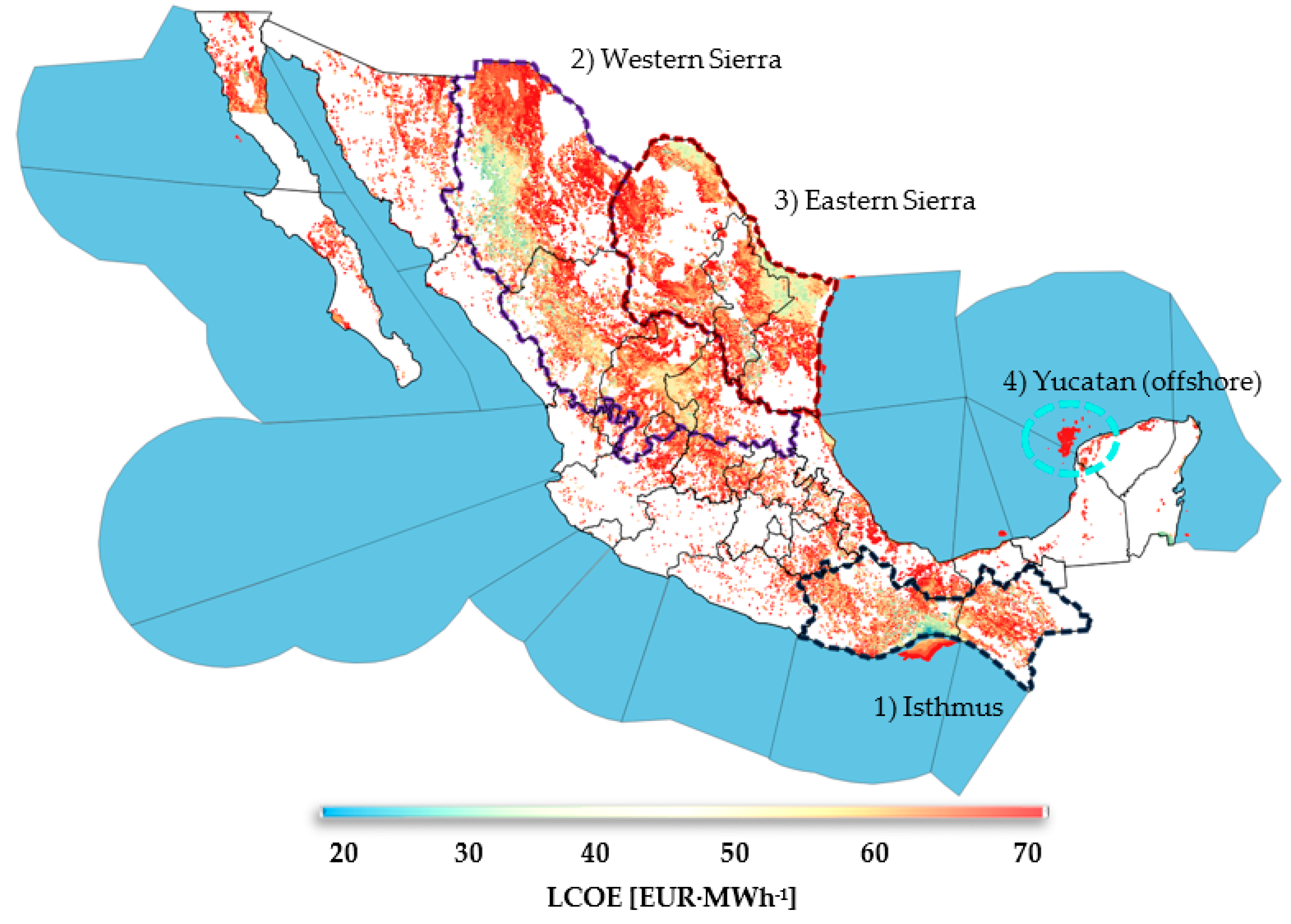
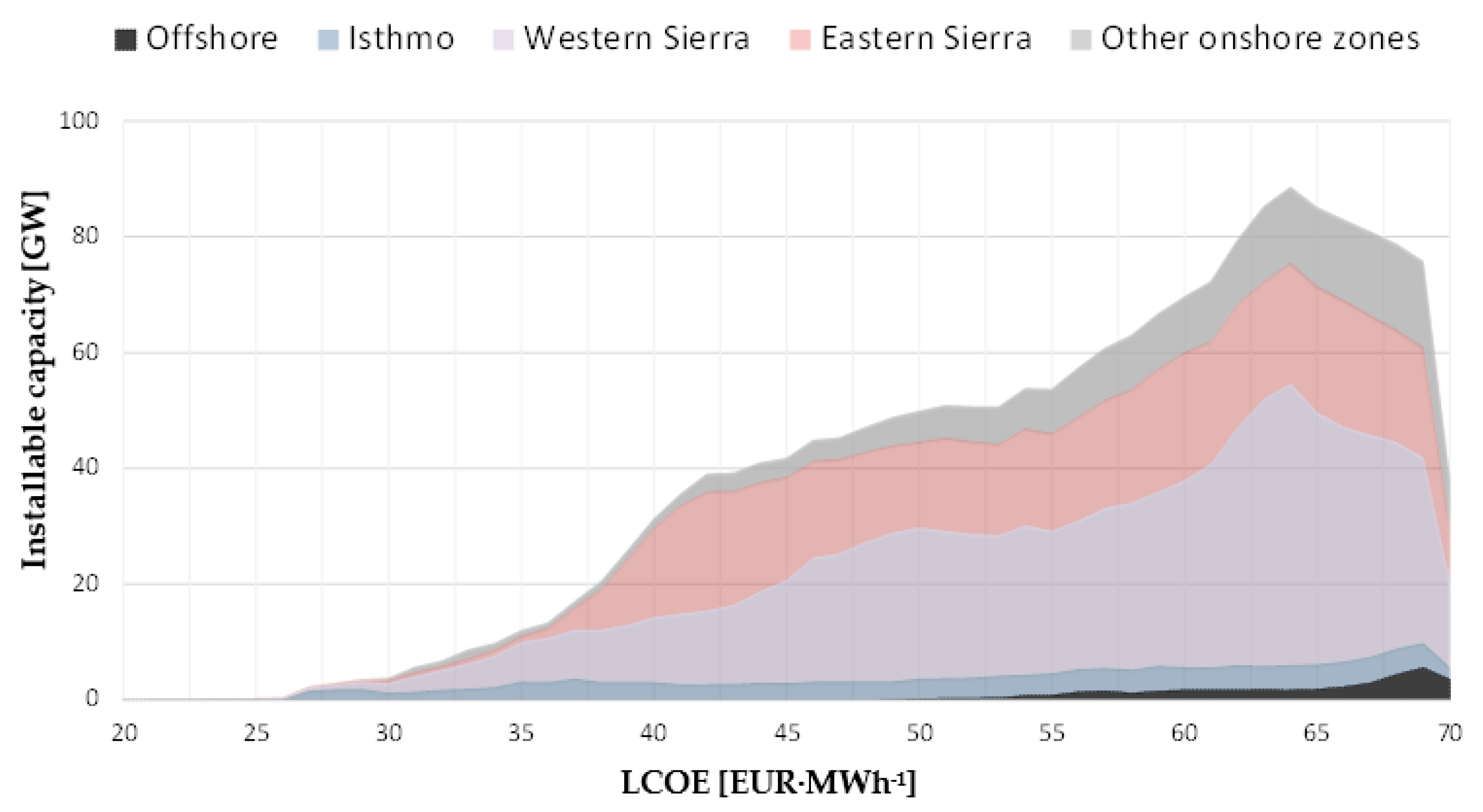
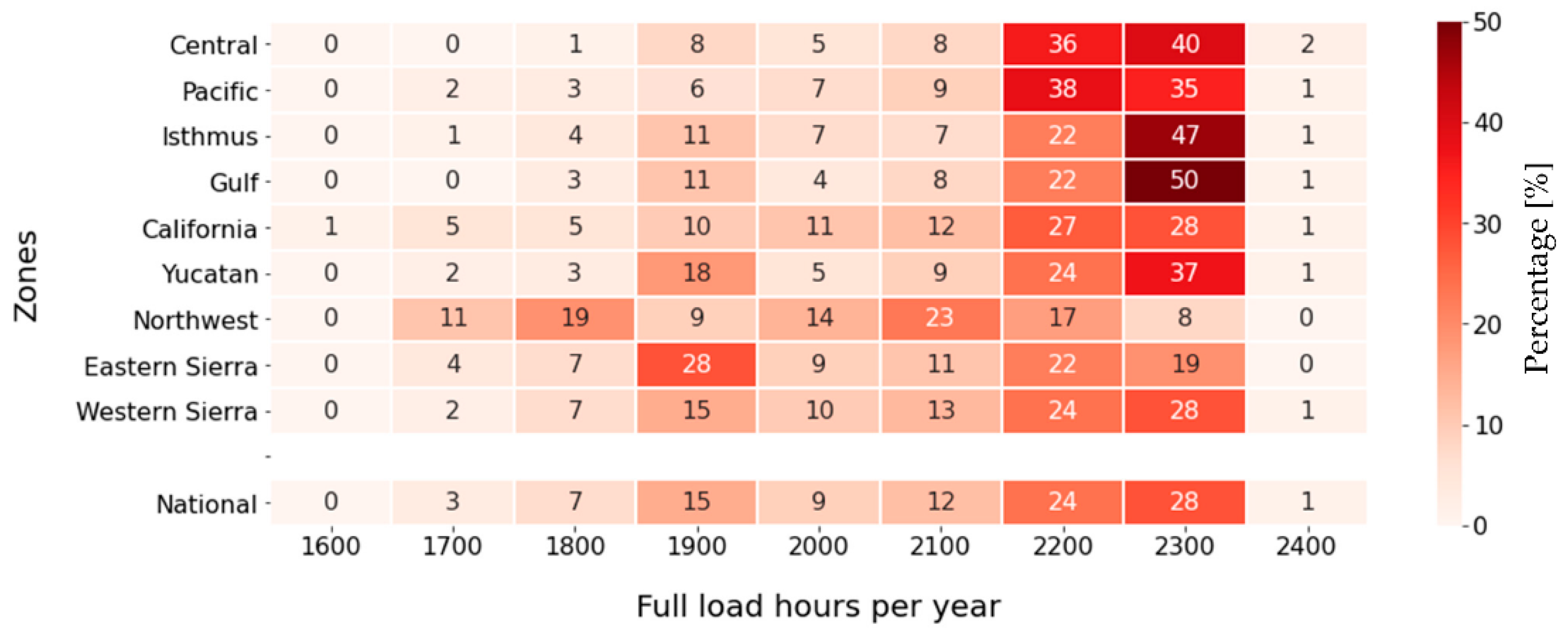
3.2.1. Wind Energy Potential and Distribution

Figure 4 shows the 39-year average LCOE from 20 (the lowest LCOE yielded) to 70 EUR·MWh−1 of onshore and offshore wind turbines. A white background is assigned to ineligible land. Four notable zones with good wind resources, all of which are mountainous, can be identified, namely: (1) The Isthmus (dotted in dark blue), where two different mountain systems create a gap that funnels and intensifies onshore wind resources towards the Pacific Ocean. This zone also covers some offshore wind potential. (2) The Western Sierra (dotted in purple), a chain of mountains that runs alongside the pacific coast through several northwestern states; (3) the Eastern Sierra (dotted in red), which is the eastern parallel with similar wind resources. Additionally, (4) a smaller area of offshore potential within the shallow waters of the Yucatan peninsula’s eastern coastal line (dotted in light blue). Due to the geospatial dependence on mountains, slope-related constraints directly affect the wind potential adjacent to these regions. Some other good wind resources coincide with the coastal line of the Gulf of Mexico, and scattered locations in both peninsulas can also be highlighted. As some of these areas are protected for environmental reasons, turbine placement is bypassed in them, and the remaining installations do not exhibit apparent clusters. Moreover, the turbine and grid infrastructure deployment needed to explore wind potential in those regions conflicts with environmentally protected areas. Figure 4 also confirms that offshore wind zones not only offer less eligible areas but also less techno-economic potential than onshore sites. Relatively higher wind speeds in far-to-shore waters do not translate into cheaper LCOEs due to higher installation caused by increased sea floor depths and distance to the coast. Consequently, the most cost-attractive offshore zone is found near the coast of the Isthmus, where it partially benefits from the isthmus’ wind funnel.
Figure 5 shows the wind capacity potential versus an LCOE of up to 70 EUR·MWh−1 grouped by zones. With the curtailment applied at 70 EUR·MWh−1, 15% of the VRES generation’s installable capacity, pertaining almost exclusively to wind energy, was filtered out, but only 8% of the total VRES power output was reduced, which confirms that the filtered-out wind turbines contribute only a small fraction of the generation potential.
Despite being relatively small relative to the size of the country, the Isthmus contains around 53% (6.5 GW) of all onshore capacity with an estimated future LCOE equal to or less than 30 EUR·MWh−1. This wind potential distribution confirms and explains why this zone alone contained around 90% (1.8 GW) of the national wind capacity as in 2019 [77]. The sunrise-facing Western Sierra (light purple) and Eastern Sierra (light red) uphills create high-speed wind corridors that can each accommodate up to 214 GW of capacity (or 37% of the total) with an LCOE of 50 EUR·MWh−1 or lower. By comparison, the smaller Isthmus zone comprises approximately 12% (63 GW) of the total capacity within the same LCOE range, whereas scattered onshore resources in the rest of the country (gray) make up the remaining 14% (83 GW). Similarly, offshore wind energy potential (in back) below 70 EUR·MWh−1 of 92 GW (97% of total) exists almost exclusively in the seas around the Isthmus and Yucatan peninsula.
Table 2 presents the values for capacity, hub height, FLH, and mean generation, corresponding to an average turbine design per geographical zone for various LCOE batches that could serve as a design reference for comparison or as modeling parameters when an optimal wind turbine design algorithm is unavailable. For onshore installations, investments and mean generation electricity production are proportional to the turbines’ baseline costs and FLH, respectively. In general, turbines in the Isthmus area have slightly larger capacities and lower hub heights due to the region’s higher wind speeds compared to those in the Western and Eastern Sierras, which have similar designs because of the similar geographical features. As the LCOE threshold increases to 50 or 70 EUR·MWh−1, average designs in the three zones tend to look similar until merging into a national average design of 4.1 MW capacity, 125 m hub height, and 126 m rotor diameter. On the other hand, the FLHs exhibit a large deviation based on the geographical zone. The FLH in the best locations, such as the Isthmus, is almost 45% bigger than the national average. Consequently, the national onshore LCOEs vary considerably, as noted in the previous figure.
Table 3 displays the average offshore turbine characteristics with an LCOE restricted to 70 EUR·MWh−1 or lower by zone. As the offshore turbines were modeled with a fixed design (see Section 2.2), investment costs varied slightly from 19 to 20.8 million EUR due to the different contributions of the distance to shore, ocean depth, and foundation type on the costing function. Nevertheless, the resulting investment costs were around four times higher than those for onshore turbines, whereas the resulting mean generation was not proportionally higher. In fact, comparing the best locations, two onshore turbines could produce around 86% of the electricity output of one offshore turbine at around half (52%) the installation cost. Therefore, the LCOE of offshore wind is considerably higher than onshore.

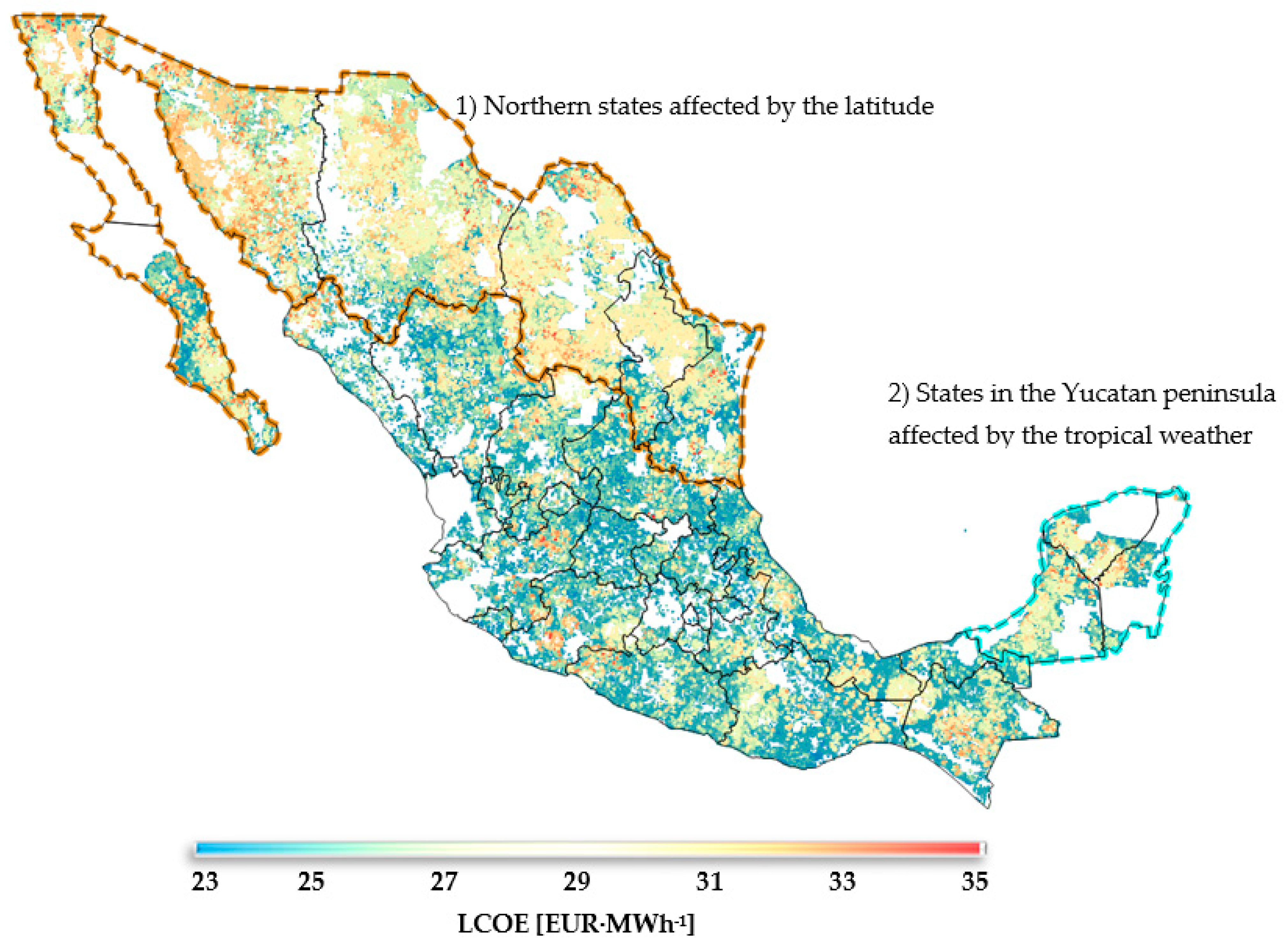
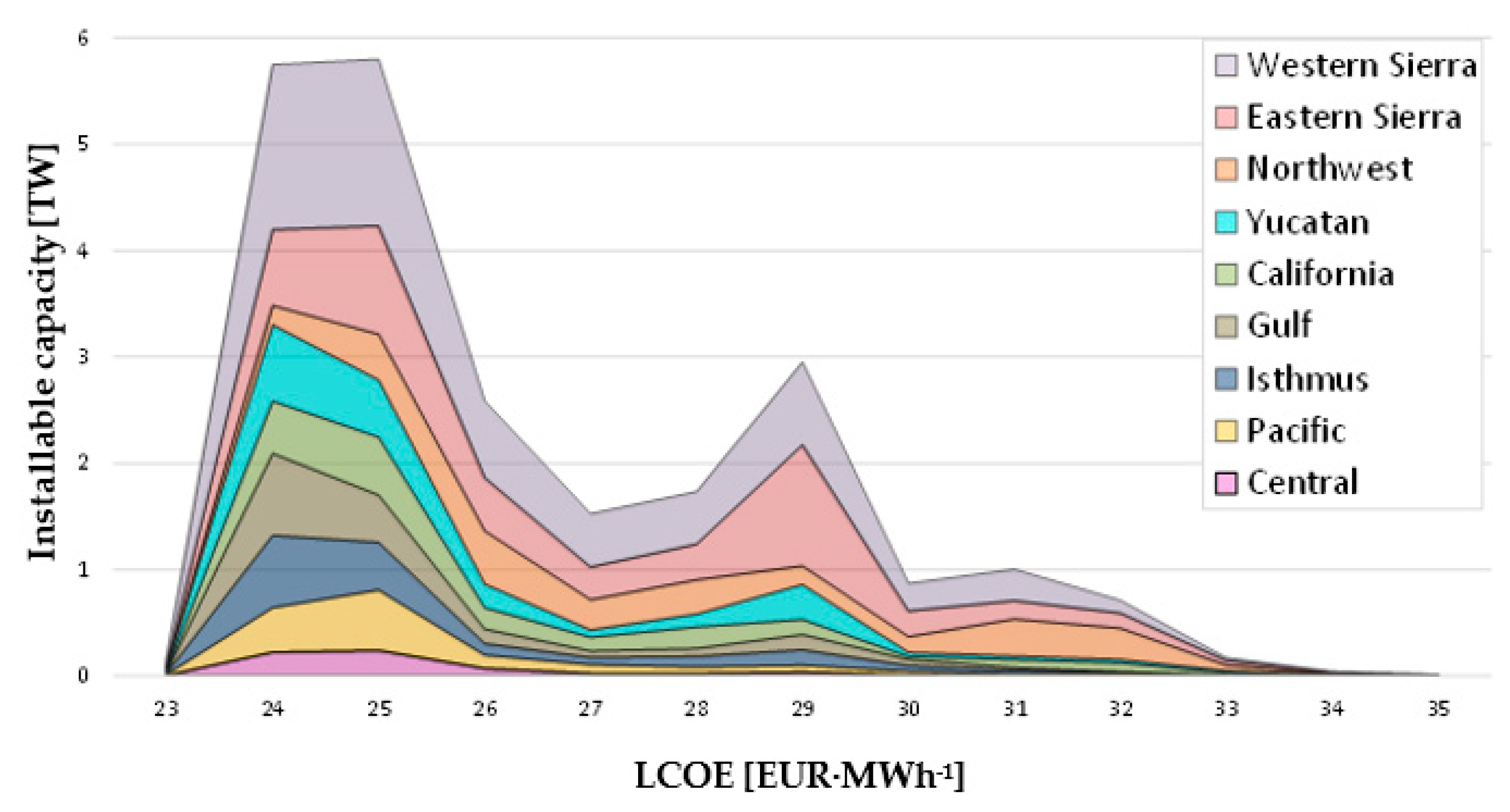
3.2.2. PV Potential and Distribution

Figure 6 shows the corresponding LCOE map for PV technologies. Overall, Mexico has large PV energy potential throughout the country. Nevertheless, two effects slightly affect this: the effect of latitude and tropical weather. PV LCOEs tend to be slightly more expensive as latitude increases due to fewer hours of sunlight throughout the year. Northern states in the proximity of the border to the U.S. (marked with a dotted yellow line) have LCOEs of approximately 30 EUR·MWh−1, whereas, towards the center, the LCOEs are mostly around 25 EUR·MWh−1. Despite this latitude effect, the eligible area for PV parks in the northern states is much larger, which leads to increased solar potential. The tropical climate also affects PV panels.
In contrast to the latitude effect, the climate in the Yucatan peninsula and most of the states along the coasts (marked by dotted blue lines) are subject to more rain and clouds that cause less FLH and therefore increase the LCOE. As there is no fundamental modeling difference between PV technologies, rooftop PV exhibits higher LCOEs than open-field due to the CAPEX difference and suboptimal orientations. Its total potential is negligible compared to open-field PV.
Figure 7 presents the PV capacity potential by LCOE and is grouped into zones. Because of the PV potential’s direct dependency on the amount of eligible land, zones with larger areas have greater PV potential. Accordingly, the northern zones, such as the Western Sierra, Eastern Sierra, and Northwest, have the greatest potential. 90% (20.8 TW) of the national capacity is within 24 and 30 EUR·MWh−1, and 41% (9.6 TW) is found at an LCOE equal to or below 25 EUR·MWh−1. All of the zones exhibit installable capacity in all of the LCOE ranges due to suboptimal terrain characteristics such as elevation, tilt, or shadows.
A different way to look at the PV potential is by considering PV parks’ FLH as a proportion of the total potential by zone, as presented in Figure 8. This makes it apparent that 2300 FLH is the predominant condition nationally, which explains the good PV generation potential across the country. On the other hand, it also indicates that within zones, there is a large difference between the highest and lowest FLH yields. Differences of around 800 to 500 FLH or +/− 12 EUR·MWh−1 between the best and worst locations can be seen in the California peninsula or the Gulf of Mexico, respectively. The differences are a consequence of particular local conditions, such as irradiance or temperature. The latitude effect discussed previously in the PV potential is even more clearly shown. The northern zones, by contrast, such as the northwestern 8% of the placements, yield 2300 FLH, whereas, in more central zones, such as the Gulf, Isthmus, or Central, the share of the same FLH batch is over 40%. Similarly, the tropical weather effect also slightly reduces the share of this FLH batch in the Yucatan peninsula (37%) compared to other zones at similar latitudes, such as the Central or Gulf (40% and 50%, respectively) regions. Unlike the wind turbines simulation, PV technologies were simulated using a single PV model, and therefore a table with an average PV park design is not provided.

4. Discussion

This section focuses on differences with the most relevant previous VRES assessment and the implications of the chosen methodology. Additionally, a brief discussion about the validation of the computational models by their authors is offered. Finally, possible ways by which the assessment can be further improved in the future are presented.
In comparison to other VRES assessments in Mexico, only five of the regional studies mentioned in the literature review can be compared to some extent to this study due to their mixed, and sometimes unstated, methodologies. Jaramillo et al. [16] concluded that 750 kW wind turbines in Baja California Sur would operate on average for 2200 FLH, producing LCOEs from 40–60 EUR·MWh−1 (1.1 USD to EUR conversion rate used [6]). In comparison, this assessment demonstrates an average of almost 3000 FLH (25% more), with LCOEs ranging from 46–50 EUR·MWh−1. The results reported herein largely coincide with Jaramillo et al.’s, despite the latter having arrived 15 years ago, but with vast differences in turbine design. Jaramillo et al. drew on comparable costs, such as a CAPEX of 1000 EUR·kW−1 and OPEX equivalent to 1% of the CAPEX, with an additional five years of economic life. The CAPEX cost estimation function utilized here also includes costs associated with grid connection and balance of system costs that were not stated as considered in Jaramillo et al. and whose impact on the LCOE could offset the performance gains of future turbine designs. In another example, the assessment for the state of Veracruz by Hernández Escobedo [18] deviates considerably from the results obtained in this assessment. The techno-economic average energy yield per turbine in this study in the same state increased by around 19% in comparison to the results of Hernández Escobedo. However, if merely a simple state average, as reported by Hernández Escobedo, is considered, a 60% yield reduction per turbine is seen here, despite the modeling of futuristic turbine designs. Further investigation and the reproducibility of Hernández Escobedo’s work is not possible as non-open source software was employed. Furthermore, Hernández Escobedo [22] also assessed another Mexican region, namely the Baja California peninsula, where a comparison was also not possible, as it is an ineligible area due to environmental protection constraints according to the LEA used in this study. Rodriguez Hernandez’s [23] assessment of the area of Mexico City concluded that there is virtually no techno-economic wind potential, which is consistent with the findings of this study. The potentials in the AZEL assessment [25] are most comparable to those in this study. Table 4 summarizes the comparison between them. In general, the AZEL estimates the total installable capacity for both open-field PV and onshore wind. This is a direct consequence of the more extensive LEA employed here that significantly reduces the maximum installable VRES capacities compared to AZEL, which only considers 11 constraints for onshore and 13 for open-field PV. Therefore, the maximum installable capacities in the AZEL assessment appear to be larger. Nevertheless, when looking at FLH or generation per installment, in this study, the performance always increased. The reason for this is that AZEL employed a power density factor to calculate national potential, whereas, in this study, the power generation was simulated for each VRES placement. Additionally, the improved VRES performance and optimal wind turbine designs were not considered in AZEL, which explains the poorer individual performance and reduces the potential gap between both assessments. Consequently, the generation and capacity potentials differ.
Another topic is the validation of the models used. In general, the validation of the models was carried out using international datasets, comparisons with other, and, when available, measured data. Here, only the final deviation percentage and conclusions of the validation are included. For more information, please refer to the original sources.
The authors of the GLAES model declare that eight studies in Europe containing LEA were replicated, and the average land differences were compared. The average land deviation found was 3.51%. As mentioned in Section 2.1, most of the input datasets were previously employed and were kept unchanged. Exceptions are official datasets published by Mexican authorities that are presumable more accurate than international sources. For these reasons, a similar land deviation can be expected and is considered acceptable for a national-wise assessment such as for Mexico by the authors of this assessment. For the simulation procedure, the work of Ryberg [32] offers time series visual comparisons against measured data, regional potential, and turbine design comparisons for the validation of onshore wind potential. The author concludes that “the model does an acceptable job at recreating the measured generation”. The same model was used also by assessing the offshore wind potential in Europe by Caglayan et al. [35], where a similar conclusion was reached. In regards to the PV simulation scheme, Ryberg [32] compared the simulation results to those found by Pfenninger et al. [74] and the Global Solar Atlas [54]. The results of the comparison show an approximate 5% temporal deviation against Pfenninger and 6% spatial deviation with Global Solar Atlas. Given the complexity of the validation procedure of both wind and PV, the reader is again encouraged to go to the original source for more information.
The VRES assessment results can vary significantly due to a number of assumptions made by their authors in the LEA, VRES simulation procedure, or techno-economical parameters incorporated. Nevertheless, new constraints could gain relevance or current ones lose it as VRES technologies are progressively deployed and increasingly interact with other activities. Consequently, the area available for VRES installations and ultimately the VRES generation potential will change as environmental, physical, sociopolitical, and economic conditions do.
A way to improve the assessment is by accessing higher-quality data. Even though the most up-to-date databases were used herein, data measurements can always be improved in the future and return results that are more precise. Other unevaluated issues arising in this assessment are disruptive technologies that can totally change the power system by revealing new energy potentials. Unfortunately, no model can predict the occurrence of these, much less their consequences. Only foreseeable technological improvements on current designs through 2050 have been captured by the design of synthetic power curves for wind turbines and PV panels with improved performance, as estimated by Ryberg [32], are considered. Increasing the simulations’ resolution (temporally and spatially) is beneficial for increasing the accuracy of the results, although its exact extent is not yet known. Hourly evaluation and 100 m spatial resolution is currently a widely accepted resolution for a country assessment and can be performed in a reasonable amount of time due to its lower computational complexity. Local conditions, such as noise tolerance, shadows, or roughness-lengths, are also left unevaluated as a trade-off.

5. Conclusions

In light of the results of this study, several conclusions can be drawn. Firstly, open-field PV is by far the most abundant and cheaper VRES in the country. The generation potential of PV energy is up to 10 times larger than the wind energy potential and is present practically all across the country. Most of the LCOEs from PV energy are below 30 EUR·MWh−1, which is less than half of most of the wind potential. Moreover, based on the generally good PV potential across the country, its deployment is likely to be highly decentralized. The development of the power system should anticipate adequate legal, economic, and technological frameworks in order to make the best use of these. A revision of the applicability of the LEA constraints and buffer zones is also recommended to capture changes in social preferences over time towards wind and PV technologies.
Secondly, the onshore wind potential is regional. Around 81% of the best wind energy potential is concentrated in three mountainous zones. This potential is enough to satisfy around 4 to 5 times the current energy demand. Given this concentrated distribution, there must be a strong emphasis on the development of future energy infrastructure, such as transmission lines, energy storage, and even renewable fuel production, in these wind energy-rich regions in order to incorporate more wind energy into the national energy system. Off-grid connections are possible too; however, the wind potential is likely to be underutilized given the low demand that is usually found in these remote areas. In contrast, bringing interconnected renewable energy projects in there would help incorporate more renewable energy into the national electricity mix. Such projects can also help overcome the other two energy challenges, such as better electricity access in remote areas and meeting Mexico’s environmental commitments.
Thirdly, in the center of the country, where the political boundaries create smaller and more densely-populated areas, there is the least techno-economic VRES potential. This limited renewable potential comes exclusively from open-field PV. Mexico City, for example, exhibits no techno-economic wind potential but around 260 MW of PV at 28 EUR·MWh−1, which is limited by land availability. At the same time, the central regions have high power consumption rates, which could increase the proclivity to deploy the existing PV potential as soon as possible. For this reason, the implementation of a higher-resolution regional model is recommended, as well as a more region-specific analysis favoring optimal PV potential utilization.
Finally, apart from the possible methodological improvements presented in the discussion section, incorporating inputs from local stakeholders in future assessments will be highly beneficial. Key players can help to better understand additional local challenges and opportunities in terms of land use, technology costs and access, legal and environmental considerations, etc., that are hard to represent in a nationwide analysis. Future studies can incorporate local data inputs when appropriate and to validate the assessments’ results to make more robust conclusions, thus, reducing the resistance to implementing new sustainable strategies.

Author Contributions

Conceptualization, E.U.P.S., S.D.R. and H.U.H.; methodology, S.D.R., E.U.P.S., H.U.H., D.S.; software, S.D.R. and E.U.P.S.; validation, S.D.R. and E.U.P.S.; formal analysis, E.U.P.S., S.D.R. and H.U.H.; investigation, E.U.P.S., S.D.R. and H.U.H.; resources, H.U.H., D.S. and M.R.; data curation, E.U.P.S., S.D.R. and H.U.H.; writing—original draft preparation, E.U.P.S., S.D.R. and H.U.H.; writing—review and editing, H.U.H., D.S. and M.R.; visualization, E.U.P.S.; supervision, S.D.R., H.U.H., D.S. and M.R.; project administration, S.D.R. and H.U.H.; funding acquisition, E.U.P.S., M.R. and D.S. All authors have read and agreed to the published version of the manuscript.

Funding

This research was funded by the CONACYT-SENER “Sustentabilidad Energética 2017” fund, grant number: 74489 and the Helmholtz Association under the Joint Initiative “Energy System 2050: A Contribution of the Research Field Energy.” The APC was funded by the Forschungszentrum Juelich GmbH.

Data Availability Statement

The research data might be obtained if legally possible by sending an e-mail to the main author. Approval for the data release by the Institute of Energy and Climate Research—Techno-economic Systems Analysis (IEK-3) of the Forschungszentrum Juelich is needed.

Conflicts of Interest

The authors have no conflict of interest to declare.

Appendix A. Earthquakes and Tsunamis as LEA Constraints

Several studies have investigated how wind turbines would behave in response to earthquakes. In 2003, Lavassas et al. [78] carried out an analysis and developed a design for a 1 MW, steel, 44 m-high wind turbine tower that corresponded to the Greek Anti-Seismic Code EAK 2000. It was concluded that seismic activity would only play a significant role in seismically hazardous areas with a combination of medium and soft placement soil. Similarly, Ritschel et al. [79] performed two types of computational simulations: one, typically used for buildings and called “modal,” as described by Clough et al. [80]; and one code specifically for wind turbines called “Flex5” [81]. The simulation was carried out to generate accelerograms in accordance with the European standard Eurocode 8 [82] for a Nordex N80 (onshore, 80 m rotor diameter, 60 m hub height, 2.5 MW output) that was installed in a seismic region in Ryuy-Cho, Japan, a site with a peak ground acceleration of 0.3 g. According to Ritschel et al., although both models returned slightly different results, with the Flex5 one featuring more bending, simulated seismic shakes were negated by the designed turbine models. Moreover, according to a 2016 literature review on wind turbines and seismic hazards by Kastanos et al. [83], there exists a consensus in the engineering community that the loads caused by earthquakes of importance for wind turbines are horizontal and wind-driven and that there is a “self-insolated effect” during the most destructive portion of an earthquake. Kastanos et al. supported their conclusions by drawing on observations of earthquakes in 1986 near an onshore wind farm in North Palm Springs, California, and in 2011 at the Kamisu offshore wind farm phase 1 in Tohoku, Japan.
Contrary to reports on hurricanes damaging wind turbines, the evidence of the effects of earthquakes can be exemplified clearly by the cases in Japan and California with offshore and onshore wind farms, respectively. In both instances, no turbine damage was reported. During the 2011 Great East Japan earthquake and tsunami (measuring 9.1 on the Richter Moment Magnitude Scale [84]), the Kamisu offshore wind farm contained seven Hitach HTW 2.0-80 wind turbines of 2 MW and with 60 m hub heights. Although the power was interrupted by grid checking after the tsunami, the wind farm continued providing power for three days following the tsunami, with no damage reported [85]. Matsunobu et al. [85] investigated the case and found that an “extreme wave + wind” is much more severe in terms of structural stress than a “Tsunami + power production” scenario, based on simulations of the Kamisu offshore phase 1 and the actual 2011 tsunami, which confirmed that the mono-pile wind turbine structures can withstand seismic vibrations. These results and observations were implemented in the design and construction of phase 2 of the same project. In this context, Bhattacharya et al. [86] noted that the use of offshore wind farms can even increase the seismic resilience of nuclear power plants, which are often close to the sea. They could also supply the power for cooling systems and would not fail for the same reasons as other emergency systems and, therefore, could help avoid a cascade of catastrophic consequences.
In the case of onshore wind, a study by Kübler et al. [87] from Swiss Re reports that in the Painted Hills onshore wind farm in California, none of the 65 wind turbines was destroyed by the earthquake in 2011. However, 48 of them had to undergo minor repairs. The wind farm is in the Riverside country, which is regarded as having a 75% likelihood of an M7.0° earthquake occurring within the next 30 years. For more local cases, Oaxaca, Mexico is a site at which wind farms have operated since 1994 [88]. On the 7th and 19th of September 2017, two notable earthquakes occurred at this site; the first measured M8.2° and the second M7.1° [89]. In both instances, none of the 1200 wind turbines were damaged [89]. Again, the power supply was also cut due to afflictions on the power lines, urban areas, and security grid issues [89].
Nevertheless, given the limited experience of only the last few decades and that not enough on-site experiments have been conducted, it cannot be concluded that wind turbines are earthquake-proof. This hazard analysis should be taken into consideration with the increased risk of a common failure of wind turbines [83]. In the case of solar technologies, during the 2011 earthquake and tsunami in Japan, existing solar panel operations were shut down due to grid problems rather than the destruction of the panels [90].
Table A1. Land constraints and buffer zones for the placement of VRES technologies in Mexico.
GroupNo.Criterion
Sub-Criterion (Optional)
Exclusion Zone (<in Meters When Not Specified)ReferencesDataset Source
Onshore WindOpen-Field PVOffshore Wind
Sociopolitical1Settlements[34]INEGI [91]
Urban1200200-
Rural800
2Agricultural Areas-0-[34]INEGI [92]
3Airports40000-[34]Osm2sh [93]
4Roads[34]INEGI [94]
Primary200--
Secondary300
5Railways200--[34]Geofabrik [95]
6Marine Shipping Routes--3000[35]ArcGIS [96]
7Power or submarine lines200-500[34,35]Geofabrik [95], NOAA [97]
8Historical sites10001000-[34]INEL [98]
9Archeological sites10001000-[34]INEL [98]
10Recreational areas10001000-[34]MapCruzin [99]
11Leisure and Camping10001000-[34]MapCruzin [99]
12Tourism10001000-[34]MapCruzin [99]
13Industrial Areas[34]MapCruzin [99], SENER
Natural Gas facilities3000-
Oil facilities300
14Mining sites2000-[34]SE [100]
15Gas lines200--[34]SENER [101]
16Power plants (>100 MW)200--[34]IEA, SENER, INEGI [102]
17Military areas10001000-AddedOsm2sh [93]
18Country borders500500-[42]INEGI [91]
19Harbors1000--AddedSENER [101]
20LNG terminals1000--AddedSENER [101]
Physical21Total slope17°10°-[34]USGS [64]
Northward slope-
22Water lines[34,35]INEGI [103]
Rivers, Canals and Brooks200--
Distance from coast1000100015,000
23Water bodies[34]INEGI [103]
Natural wells/Cenotes10001000-
Lakes and lagoons400
Dams, Flooding zones200
24Woodlands3000-[34]INEGI [92]
25Jungles3000-AddedINEGI [92]
26Wetlands[34]INEGI [92]
Marshland10001000-
Swap
27Land elevation/Ocean depth300017501000[34]USGS [64], GEBCO [104]
28Geothermal sites200200-AddedINEGI [105]
29Active volcanoes20002000-AddedINEGI [105]
30Hurricanes (>category 3)30,00050,00030,000AddedNOAA [47]
Conservation31Protected Fauna, Flora and Habitats (FFH)[34,35]World database on Protected Areas [106], UNEP-WCMC [107]
Habitats10001000-
Bird conservation
Biospheres
Wilderness
Marine life--1000
Coral reefs
32Protected areas[34]World Database on Protected Areas [106]
Landscapes and Reserves10001000-
Parks and Monuments
Econo-mical33Access>30,000>30,000-[34]INEGI [94]
34Resources (wind speed)4 m/s-4 m/s[34]GWA [59]

References

  1. IRENA. Renewable Energy Capacity Highlights 2020; IRENA: Masdar City, Abu Dhabi, 2020; p. 3. [Google Scholar]
  2. Ajadi, T.; Boyle, R.; Strahan, D.; Kimmel, M.; Collins, B.; Cheung, A.; Becker, L. Global Trends in Renewable Energy Investment 2019; Frankfurt School-UNEP Centre: Frankfurt; Germany, 2019. [Google Scholar]
  3. IEA. Renewables 2019; International Energy Agency: Paris, France, 2019. [Google Scholar]
  4. The United Nations. Adoption of the Paris Agreement in the Conference to the Parties Twenty-First Session; The United Nations: Paris, France, 2015. [Google Scholar]
  5. The World Bank. Classifing Countries by Income; The World Bank: Washington, DC, USA, 2019; Available online: https://datatopics.worldbank.org/world-development-indicators/stories/the-classification-of-countries-by-income.html (accessed on 7 November 2019).
  6. The World Bank. GDP (Current US$). 2019. Available online: https://data.worldbank.org/indicator/NY.GDP.MKTP.CD?view=chart (accessed on 1 June 2020).
  7. U.S. Census Bureau. World Population. 2020. Available online: https://www.census.gov/popclock/print.php?component=counter (accessed on 1 June 2020).
  8. International Energy Agency. Energy Policies Beyond IEA Countries: Mexico 2017; International Energy Agency: Paris, France, 2017; Available online: https://www.iea.org/reports/energy-policies-beyond-iea-countries-mexico-2017 (accessed on 12 November 2019).
  9. Gobierno de México. Compromisos De Mitigación Y Adaptación Ante El Cambio Climático Para El Periodo 2020-2030, New York, USA; 2014. Available online: https://www.gob.mx/cms/uploads/attachment/file/162974/2015_indc_esp.pdf (accessed on 24 November 2019).
  10. The Union of Concerned Scientists. Each Country’s Share of CO2 Emissions; The Union of Concerned Scientists: Cambridge, MA, USA, 2019; Available online: https://www.ucsusa.org/resources/each-countrys-share-co2-emissions (accessed on 15 September 2020).
  11. Secretaría de Energía. Programa de Desarrollo del Sistema Eléctrico Nacional 2018–2032 (PRODESEN); Gobierno de Mexico: Mexico City, Mexico, 2018.
  12. Gobierno de México. Plan Nacional de Desarrollo 2001-2006; Gobierno de Mexico: Mexico City, Mexico, 2001.
  13. The United Nations. World Population Prospects 2019; The United Nations: New York, NY, USA, 2019. [Google Scholar]
  14. Hawksworth, J.; Chan, D. The World in 2050: Will the Shift in Global Economic Power Continue? PwC: Belfast, UK, 2015. [Google Scholar]
  15. Schwartz, M.N.; Elliott, D.L. Mexico Wind Resource Assessment Project; National Renewable Energy Laboratory: Washington, DC, USA, May 1995.
  16. Jaramillo, O.A.; Saldana, R.; Miranda, U. Wind power potential of Baja California Sur, México. Renew. Energy 2004, 29, 2087–2100. [Google Scholar] [CrossRef]
  17. Hernández-Escobedo, Q.; Manzano-Agugliaro, F.; Zapata-Sierra, A. The wind power of Mexico. Renew. Sustain. Energy Rev. 2010, 14, 2830–2840. [Google Scholar] [CrossRef]
  18. Hernández-Escobedo, Q.; Espinosa-Arenal, F.; Saldaña-Flores, R.; Rivera-Blanco, C. Evaluación del potencial eólico para la generación de energía eléctrica en el Estado de Veracruz, México. Dyna 2012, 79, 215–221. [Google Scholar]
  19. Figueroa-Espinoza, B.; Salles, P.; Zavala-Hidalgo, J. On the wind power potential in the northwest of the Yucatan Peninsula in Mexico. Atmosfera 2014, 77–89. [Google Scholar] [CrossRef] [Green Version]
  20. Carrasco-Díaz, M.; Rivas, D.; Orozco-Contreras, M.; Sánchez-Montante, O. An assessment of wind power potential along the coast of Tamaulipas, northeastern Mexico. Renew. Energy 2015, 78, 295–305. [Google Scholar] [CrossRef]
  21. Carreón-Sierra, S.; Salcido, A.; Castro, T.; Celada-Murillo, A.T. Cluster analysis of the wind events and seasonal wind circulation patterns in the Mexico City region. Atmosphere 2015, 6, 1006–1031. [Google Scholar] [CrossRef] [Green Version]
  22. Hernandez-Escobedo, Q. Wind energy assessment for small urban communities in the Baja California Peninsula, Mexico. Energies 2016, 9, 805. [Google Scholar] [CrossRef]
  23. Rodriguez-Hernandez, O.; Martinez, M.; Lopez-Villalobos, C.; Garcia, H.; Campos-Amezcua, R. Techno-economic feasibility study of small wind turbines in the Valley of Mexico metropolitan area. Energies 2019, 12, 890. [Google Scholar] [CrossRef] [Green Version]
  24. Ryberg, D.S.; Caglayan, D.G.; Schmitt, S.; Linßen, J.; Stolten, D.; Robinius, M. The future of European onshore wind energy potential: Detailed distribution and simulation of advanced turbine designs. Energy 2019, 182, 1222–1238. [Google Scholar] [CrossRef]
  25. Secretaría de Energía. Atlas Nacional de Zonas con alto Potencial de Energías Limpias (AZEL). 2019. Available online: dgel.energia.gob.mx/azel/ (accessed on 10 November 2019).
  26. McKenna, R.; Hollnaicher, S.; Fichtner, W. Cost-potential curves for onshore wind energy: A high-resolution analysis for Germany. Appl. Energy 2014, 115, 103–115. [Google Scholar] [CrossRef]
  27. Jäger, T.; McKenna, R.; Fichtner, W. The feasible onshore wind energy potential in Baden-Württemberg: A bottom-up methodology considering socio-economic constraints. Renew. Energy 2016, 96, 662–675. [Google Scholar] [CrossRef]
  28. Pfenninger, S.; DeCarolis, J.; Hirth, L.; Quoilin, S.; Staffell, I. The importance of open data and software: Is energy research lagging behind? Energy Policy 2017, 101, 211–215. [Google Scholar] [CrossRef]
  29. National Aeronautics and Space Administration. Modern-Era Retrospective analysis for Research and Applications, Version 2. NASA Goddard Earth Sciences (GES) Data and Information Services Center (DISC). 2019. Available online: https://disc.gsfc.nasa.gov/datasets?keywords=%22MERRA-2%22&page=1&source=Models%2FAnalysesMERRA-2 (accessed on 15 April 2020).
  30. Robinius, M.; Otto, A.; Syranidis, K.; Ryberg, D.S.; Heuser, P.; Welder, L.; Grube, T.; Markewitz, P.; Tietze, V.; Stolten, D. Linking the power and transport sectors—Part 2: Modelling a sector coupling scenario for Germany. Energies 2017, 10, 957. [Google Scholar] [CrossRef] [Green Version]
  31. Robinius, M. Strom-und Gasmarktdesign zur Versorgung des Deutschen Straßenverkehrs mit Wasserstoff zur Versorgung des Deutschen Straßenverkehrs mit Wasserstoff Von der Fakultät für Maschinenwesen der; RWTH Aachen: Aachen, Germany, 2015; p. 300. [Google Scholar]
  32. Ryberg, D.S. Generation Lulls from the Future Potential of Wind and Solar Energy in Europe; RWTH Aachen: Aachen, Germany, 2019; p. 316. [Google Scholar]
  33. Ryberg, D.S.; Tulemat, Z.; Stolten, D.; Robinius, M. Uniformly constrained land eligibility for onshore European wind power. Renew. Energy 2020, 146, 921–931. [Google Scholar] [CrossRef]
  34. Ryberg, D.S.; Robinius, M.; Stolten, D. Evaluating land eligibility constraints of renewable energy sources in Europe. Energies 2018, 11, 1246. [Google Scholar] [CrossRef] [Green Version]
  35. Caglayan, D.G.; Ryberg, D.S.; Heinrichs, H.; Linßen, J.; Stolten, D.; Robinius, M. The techno-economic potential of offshore wind energy with optimized future turbine designs in Europe. Appl. Energy 2019, 255, 113794. [Google Scholar] [CrossRef]
  36. Fingersh, L.; Hand, M.; Laxson, A. Wind Turbine Design Cost and Scaling Model, Nrel. 2006. Available online: https://www.nrel.gov/docs/fy07osti/40566.pdf (accessed on 23 April 2020).
  37. Maness, M.; Maples, B.; Smith, A. NREL Offshore Balance-of-System Model. January 2017. Available online: https://www.nrel.gov/docs/fy17osti/66874.pdf (accessed on 23 April 2020).
  38. Centro Nacional de Control de Energía. Historia de Precios de Energía. 2017. Available online: https://www.cenace.gob.mx/SIM/VISTA/REPORTES/H_RepPreEnergiaSisMEM.aspx?N=29&opc=divCssPreEnergia&site=Preciosdelaenergía/PreciosdeNodosDistribuidos/MTR/Diarios&tipoArch=C&tipoUni=SIN&tipo=Diarios&nombrenodop=PreciosdeNodosDistribuidos (accessed on 18 October 2020).
  39. Ryberg, D.S. Geospatial Land Availability for Energy Systems (GLAES). 2018. Available online: https://github.com/FZJ-IEK3-VSA/glaes (accessed on 5 February 2021).
  40. Van Hertem, D.; Ghandhari, M. Multi-terminal VSC HVDC for the European supergrid: Obstacles. Renew. Sustain. Energy Rev. 2010, 14, 3156–3163. [Google Scholar] [CrossRef]
  41. Klokan Technologies GmbH. Coordinate Systems Worldwide. 2020. Available online: https://epsg.io/6362 (accessed on 2 February 2021).
  42. Heuser, P.M.; Ryberg, D.S.; Grube, T.; Robinius, M.; Stolten, D. Techno-economic analysis of a potential energy trading link between Patagonia and Japan based on CO2 free hydrogen. Int. J. Hydrog. Energy 2019, 44, 12733–12747. [Google Scholar] [CrossRef]
  43. Ryberg, D.S.; Robinius, M.; Stolten, D. Methodological Framework for Determining the Land Eligibility of Renewable Energy Sources. arXiv 2017, arXiv:1712.07840. [Google Scholar]
  44. Secretaría de Energía Evaluación Ambiental y Social Evaluacion Ambiental y Social Estratégica Para el Desarrollo Eólico en el sur del Istmo de Tehuantepec. pp. 1–33. 2015. Available online: https://www.gob.mx/cms/uploads/attachment/file/136647/18439_EASE_E_lico_Tehuantepec_Resumen_ejecutivo_espa_ol.pdf (accessed on 7 November 2020).
  45. Capra, L.; Gavilanes-Ruiz, J.C.; Bonasia, R.; Saucedo-Giron, R.; Sulpizio, R. Re-assessing volcanic hazard zonation of Volcán de Colima, México. Nat. Hazards 2015, 76, 41–61. [Google Scholar] [CrossRef]
  46. Weston, D. Vestas Scales up to 4.2MW, Wind. Mon. 2017. Available online: https://www.windpowermonthly.com/article/1437274/vestas-scales-42mw (accessed on 1 August 2020).
  47. Knapp, K.R.; Kruk, M.C.; Levinson, D.H.; Diamond, H.J.; Neumann, C.J. The international best track archive for climate stewardship (IBTrACS). Bull. Am. Meteorol. Soc. 2010, 91, 363–376. [Google Scholar] [CrossRef]
  48. Lejeune, P.; Feltz, C. Development of a decision support system for setting up a wind energy policy across the Walloon Region (southern Belgium). Renew. Energy 2008, 33, 2416–2422. [Google Scholar] [CrossRef]
  49. Ramírez-Rosado, I.J.; García-Garrido, E.; Fernández-Jiménez, L.A.; Zorzano-Santamaría, P.J.; Monteiro, C.; Miranda, V. Promotion of new wind farms based on a decision support system. Renew. Energy 2008, 33, 558–566. [Google Scholar] [CrossRef] [Green Version]
  50. Ummel, K.; Wheeler, D. Desert Power: The Economics of Solar Thermal Electricity Desert Power: The Economics of Solar Thermal Electricity For Europe, North Africa, and the Middle East. 2008. Available online: https://cgdev.org/sites/default/files/1417884_file_Desert_Power_FINAL_WEB.pdf (accessed on 28 September 2020).
  51. Ryberg, D.S.; Caglayan, D.G. RESKit—Renewable Energy Simulation Toolkit for Python; RESKit: Jülich, Germany, 2019. [Google Scholar]
  52. Stehly, T.; Heimiller, D.; Scott, G. Cost of Wind Energy Review; NREL: Golden, CO, USA, 2016; pp. 23–40.
  53. Maples, B.; Hand, M.; Musial, W. Comparative Assessment of Direct Drive High Temperature Superconducting Generators in Multi-Megawatt Class Wind Turbines; NREL: Golden, CO, USA, 2010. [CrossRef] [Green Version]
  54. Solargis, S.R.O.; The World Bank Group. Global Solar Atlas 2.0, a Free, Web-Based Application is Developed and Operated by the Company Solargis s.r.o. on behalf of the World Bank Group, Utilizing Solargis Data, with Funding Provided by the Energy Sector Management Assistance Program (ESMAP). Fo. 2019. Available online: https://globalsolaratlas.info (accessed on 16 February 2021).
  55. Fraunhofer ISE. Current and Future Cost of Photovoltaics; Fraunhofer ISE: Freiburg im Breisgau, Germany, 2015. [Google Scholar]
  56. Go Solar California, “PV Module List—Full Data”. September 2018. Available online: http://www.gosolarcalifornia.ca.gov/equipment/pvmodules.php (accessed on 16 February 2020).
  57. Caglayan, D.; Heinrichs, H.; Robinius, M.; Stolten, D. Robust Design of a Future 100% Renewable European Energy Supply System with Hydrogen Infrastructure. 2020. Available online: 10.20944/preprints202010.0417.v1 (accessed on 16 February 2020).
  58. Sarmiento, L.; Burandt, T.; Löffler, K.; Oei, P.Y. Analyzing scenarios for the integration of renewable energy sources in the Mexican energy system—an application of the Global Energy System Model (GENeSys-MOD). Energies 2019, 12, 3270. [Google Scholar] [CrossRef] [Green Version]
  59. Technical University of Denmark; The World Bank Group. Global Wind Atlas 3.0, a Free, Web-Based Application Developed, Owned and Operated by the Technical University of Denmark (DTU). The Global Wind Atlas 3.0 Is Released in Partnership with the World Bank Group, Utilizing Data Provided by Vortex, Using Fundi. 2019. Available online: https://globalwindatlas.info/ (accessed on 21 November 2020).
  60. Silva, J.; Ribeiro, C.; Guedes, R. Roughness Length Classification of Corine Land Cover Classes; Megajoule Consultants: Maia, Portugal, 2007. [Google Scholar]
  61. Copernicus (European Union’s Earth Observation Programme). Corine Land Cover (CLC) 2000, Version 2018. Copernicus. 2018. Available online: http://land.copernicus.eu/pan-european/corine-land-cover/clc-2000/view (accessed on 25 February 2021).
  62. International Electrotechnical Commision (ICE). IEC 61400-12-1:2017. 2017, p. 558. Available online: https://webstore.iec.ch/publication/26603 (accessed on 25 February 2021).
  63. Reda, I.; Andreas, A. Solar Position Algorithm SPA. Natl. Renew. Energy Lab. Tech. Rep. 2008, 76, 577–589. [Google Scholar] [CrossRef] [Green Version]
  64. Danielson, J.J.; Gesch, D.B. Global Multi-Resolution Terrain Elevation Data 2010 (GMTED2010); Earth Resources Observation and Science (EROS) Center: Sioux Falls, SD, USA, 2011. [Google Scholar]
  65. Spencer, J.W. Fourier Series Representation of the Position of the Sun; Commonwealth Scientific and Industrial Research Organisation (CSIRO); Victoria, Australia, 1973. Search 1971, 2, 172. [Google Scholar]
  66. Kasten, F.; Young, A.T. Revised optical air mass tables and approximation formula; Optical Society of America. Appl. Opt. 1989, 28, 4735–4738. [Google Scholar] [CrossRef]
  67. Perez, R.R.; Ineichen, P.; Maxwell, E.L.; Seals, R.D.; Zelenka, A. Dynamic global-to-direct irradiance conversion models. ASHRAE Trans. 1992, 98, 354–369. [Google Scholar]
  68. Myers, D.R. Solar Radiation: Practical Modeling for Renewable Energy Applications; CRC Press: Boca Raton, FL, USA, 2017. [Google Scholar]
  69. Perez, R.; Ineichen, P.; Seals, R.; Michalsky, J.; Stewart, R. Modeling daylight availability and irradiance components from direct and global irradiance. Sol. Energy 1990, 44, 271–289. [Google Scholar] [CrossRef] [Green Version]
  70. Perez, R.; Seals, R.; Ineichen, P.; Stewart, R.; Menicucci, D. A new simplified version of the perez diffuse irradiance model for tilted surfaces. Sol. Energy 1987, 39, 221–231. [Google Scholar] [CrossRef] [Green Version]
  71. De Soto, W.; Klein, S.A.; Beckman, W.A. Improvement and validation of a model for photovoltaic array performance. Sol. Energy 2006, 80, 78–88. [Google Scholar] [CrossRef]
  72. Brandemuehl, M.J.; Beckman, W.A. Transmission of diffuse radiation through CPC and flat plate collector glazings. Sol. Energy 1980, 24, 511–513. [Google Scholar] [CrossRef]
  73. King, D.L.; Boyson, W.E.; Kratochvil, J.A. Photovoltaic Array Performance Model; Sandia Rep. No. 2004-3535; Department of Energy: Washington, DC, USA, 2004. [Google Scholar] [CrossRef] [Green Version]
  74. Pfenninger, S.; Staffell, I. Long-term patterns of European PV output using 30 years of validated hourly reanalysis and satellite data. Energy 2016, 114, 1251–1265. [Google Scholar] [CrossRef] [Green Version]
  75. Zweifel, P.; Praktiknjo, A.; Erdmann, G. Energy Economics: Theory and Applications; Springer: Berlin, Germany, 2017. [Google Scholar]
  76. Hirth, L. The market value of variable renewables. The effect of solar wind power variability on their relative price. Energy Econ. 2013, 38, 218–236. [Google Scholar] [CrossRef] [Green Version]
  77. El Financiero. Parques Eólicos en México; El Financiero Publishing House: Mexico City, Mexico, 2019; p. 1. [Google Scholar]
  78. Lavassas, I.; Nikolaidis, G.; Zervas, P.; Efthimiou, E.; Doudoumis, I.N.; Baniotopoulos, C.C. Analysis and design of the prototype of a steel 1-MW wind turbine tower. Eng. Struct. 2003, 38, 218–236. [Google Scholar] [CrossRef]
  79. Ritschel, U.; Warnke, I.; Kirchner, J.; Meussen, B. Wind Turbines and Earthquake; Windrad Engineering GmbH; Nordex Energy GmbH: Zweedorf, Germany, 2003. [Google Scholar]
  80. Clough, R.W.; Penzien, J. Dynamics of Structures, 3rd ed.; CRC Press: Boca Raton, FL, USA, 2013. [Google Scholar]
  81. Øye, S. Dynamic Stall Simulated as Time Lag of Separation. In Proceedings of the Fourth IEA Symposium on the Aerodynamics of Wind Turbines, Rome, Italy, 20–21 November 1990. [Google Scholar]
  82. Herrmann, H.; Bucksch, H. Eurocode 8—Design of structures for earthquake resistance. In Dictionary Geotechnical Engineering/Wörterbuch GeoTechnik; Springer: Berlin/Heidelberg, Germany, 2014. [Google Scholar]
  83. Katsanos, E.I.; Thöns, S.; Georgakis, C. Wind Turbines and Seismic Hazard: A State-of-the-Art Review. Wind Energy 2016. Available online: https://0-onlinelibrary-wiley-com.brum.beds.ac.uk/doi/epdf/10.1002/we.1968 (accessed on 10 October 2020). [CrossRef] [Green Version]
  84. Mimura, N.; Yasuhara, K.; Kawagoe, S.; Yokoki, H.; Kazama, S. Damage from the Great East Japan Earthquake and Tsunami—A quick report. Mitig. Adapt. Strateg. Glob. Chang. 2011, 16, 803–818. [Google Scholar] [CrossRef] [Green Version]
  85. Matsunobu, T.; Inoue, S.; Tsuji, Y.; Yoshida, K.; Komatsuzaki, M. Seismic Design of Offshore Wind Turbine Withstands Great East Japan Earthquake and Tsunami. J. Energy Power Eng. 2014, 8. [Google Scholar] [CrossRef] [Green Version]
  86. Bhattacharya, S.; Goda, K. Use of offshore wind farms to increase seismic resilience of Nuclear Power Plants. Soil Dyn. Earthq. Eng. 2016, 80, 65–68. [Google Scholar] [CrossRef] [Green Version]
  87. Kübler, O.; Renggli, D.; Meyer, S.; Benz, G.O. Wind Farms: Harvesting Energy on Shaky Grounds and in Stormy Seas. 2013. Available online: http://www.swissre.com/library/expertise-publication/Mind_the_risk_a_global_ranking_of_cities_un- (accessed on 10 October 2020).
  88. AMEE. Panorama General de la Energía Eólica en México. 2010. Available online: https://amdee.org/Amdee/AMDEE_presentacion_esp.pdf (accessed on 10 October 2020).
  89. El Financiero. Sismos ‘Noquean’ a Energía Eólica. 2017. Available online: https://www.elfinanciero.com.mx/economia/sismos-noquean-a-energia-eolica (accessed on 10 October 2020).
  90. Schulle, K. Earthquake’s Effect on the Solar Energy Industry, Seek. Alpha. 2011. Available online: https://seekingalpha.com/article/258262-earthquakes-effect-on-the-solar-energy-industry (accessed on 10 October 2020).
  91. Instituto Nacional de Estadística Geografía e Informática (INEGI). Marco Geoestadístico Nacional. 2017 [Dataset]. Available online: https://www.inegi.org.mx/temas/mg/ (accessed on 4 October 2020).
  92. INEGI. Conjunto de Datos Vectoriales de la Carta de Uso del Suelo y Vegetación, Escala 1:250000, Serie VI (Continuo Nacional) [Dataset]. Available online: https://www.inegi.org.mx/temas/mg/ (accessed on 4 October 2020).
  93. Osm2shp. Open Street Maps Shape Files. Available online: http://osm2shp.ru/ (accessed on 14 November 2020).
  94. Instituto Nacional de Estadística Geografía e Informática (INEGI). Red Nacional de Caminos 2019. 2019. Available online: https://www.inegi.org.mx/temas/viascomunicacion/ (accessed on 14 November 2020).
  95. Open Street Map (OSM). Geofabrik Download Server; Geofabrik GmbH: Karlsruhe, Germany, 2018. [Google Scholar]
  96. CIA. Map of the World Oceans. 2012. Available online: https://www.arcgis.com/home/item.html?id=12c0789207e64714b9545ad30fca1633 (accessed on 1 May 2020).
  97. National Oceanic and Atmospheric Administration. Submarine Cables 2019. 2019. Available online: https://data.noaa.gov/dataset/dataset/submarine-cables (accessed on 1 May 2020).
  98. Secretaria de Energía. Inventario Nacional De Energías Limpias. 2017. Available online: https://dgel.energia.gob.mx/qa/INEL/INELV5/index.html (accessed on 11 November 2020).
  99. Mapcruzin. Mexico Shapefiles. 2019. Available online: https://mapcruzin.com/free-mexico-maps.htm (accessed on 1 May 2020).
  100. Secretaría de Economía. Mexico Mining Concessions. 2015. Available online: https://hub.arcgis.com/datasets/f4bebb67213b4d958938521691c97970_3 (accessed on 11 November 2020).
  101. Secretaría de Energía. Infraestructura de Gas Natural en México. 2019. Available online: https://www.google.de/maps/d/edit?mid=1NQYs864qTUl5GKLecSY-8jY2h5u9EtVP&ll=22.60802046476938%2C-105.31052626045897&z=5 (accessed on 11 November 2020).
  102. Secretaría de Energía. Mapa Energético de America del Norte. SENER, IEA, INEGI. 2019. Available online: http://gaia.inegi.org.mx/mdm-clientna/ (accessed on 14 May 2020).
  103. Instituto Nacional de Estadística Geografía e Informática (INEGI). Cuerpos de Agua. 2009. Available online: https://www.inegi.org.mx/app/biblioteca/ficha.html?upc=889463598435 (accessed on 11 November 2020).
  104. Mayer, L.; Jakobsson, M.; Allen, G.; Dorschel, B.; Falconer, R.; Ferrini, V.; Lamarche, G.; Snaith, H.; Weatherall, P. The Nippon Foundation-GEBCO seabed 2030 project: The quest to see the world’s oceans completely mapped by 2030. Geosciences 2018, 8, 63. [Google Scholar] [CrossRef] [Green Version]
  105. Instituto Nacional de Estadística Geografía e Informática (INEGI). Conjunto de Datos Vectoriales Geológicos. 2002. Available online: https://www.inegi.org.mx/temas/usosuelo/ (accessed on 7 March 2021).
  106. IUCN; UNEP-WCMC. Protected Planet: The World Database on Protected Areas (WDPA) Cambridge, UK: UNEP-WCMC and IUCN [Dataset]. 2019. Available online: www.protectedplanet.net (accessed on 15 December 2019).
  107. UNEP-WCMC; WorldFish Centre; WRI; TNC. Global Distribution of Warm-Water Coral Reefs, Compiled from Multiple Sources Including the Millennium Coral Reef Mapping Project. Version 4.0. Includes Contributions from IMaRS-USF and IRD (2005), IMaRS-USF. UNEP-WCMC, WorldFish Centre, WRI, TNC. 2018. Available online: https://data.unep-wcmc.org/datasets/1 (accessed on 20 January 2021).
Figure 1. Mexican territory by state division and regional classification.
Energies 14 05779 g001
Figure 2. The distribution of available land for the placement of wind turbines.
Energies 14 05779 g002
Figure 3. The distribution of available land for the placement of PV parks.
Energies 14 05779 g003
Figure 4. Wind potential distribution.
Energies 14 05779 g004
Figure 5. Wind potential by zone according to the yielded LCOE.
Energies 14 05779 g005
Figure 6. PV techno-economic potential distribution.
Energies 14 05779 g006
Figure 7. PV potential by zone according to the yielded LCOE.
Energies 14 05779 g007
Figure 8. PV full load hours by zone.
Energies 14 05779 g008
Table 1. VRES techno-economic parameters used.
ParameterOnshore TurbinesOffshore TurbinesOpen-Field PVRooftop PVUnits
Turbine capacity or PV Model(3.2–5.9) MW *9.4 MWWinaico WSx-240P6 (fixed tilt)LG 360Q1C-A5-
CAPEX(1090–1350) *(1570–10,000) *500800EUR·kW−1
OPEX221.71.7% of CAPEX
Economic life20252525years
Hub height(88–185) *135--m
Rotor diameter136210--m
Efficiency--2430%
Technology--PolycrystallineMono-crystalline-
Area coverage(185–100) *187206.67m2·kW−1
WACC0.080.080.080.08-
Reference[24][35][32][32]
* Range of values obtained by applying technology design correlations and costing algorithms according to the local terrain and weather characteristics incorporated in RESKit [51].
Table 2. Average design characteristics of onshore wind turbines grouped by regional zone and LCOE batch.
LCOE Batch
(EUR·MWh−1)
ZonesAverage Turbine
Capacity (MW)
Hub Height
(m)
FLH
(h/year)
Installable
Capacity (GW)
Annual Energy Yield (TWh/a)
(20–30)Isthmus5.0924550730
Western Sierra4.8984500417
Eastern Sierra4.7102450016
(30–50)Isthmus4.4115325057190
Western Sierra4.41153050248760
Eastern Sierra4.41153050212650
(50–70)Isthmus3.9136235081190
Western Sierra4.112522506581500
Eastern Sierra4.11252250385870
(20–70)National4.1125250019004800
Table 3. Average design characteristics of offshore wind turbines by zone.
Zones Where
LCOE ≤ 70
EUR·MWh−1
Distance to Shore (km)Ocean Depth (m)Foundation Type PreferenceInvestment
(Million EUR)
FLH (h/year)Installable
Potential (GW)
Annual Energy Yield (TWh/a)
Isthmus32135Spar (66%)20.8409025100
Yucatan44232Monopile (100%)19338540150
Table 4. VRES potential comparison against government estimates.
ParameterVRESAZEL
Scenario 3
Techno-Economic Potential
in This Study
∆ (%)Possible Reasons
Capacity
(TW)
Open-field PV33.523.3−30More extensive LEA
Onshore wind2.81.9−32
Generation
(PWh)
Open-field PV60.649.2−32VRES simulation procedure and higher capacities
Onshore wind6.94.8−30
FLHs
(h/year)
Open-field PV18202118+16Improved VRES performance
Onshore wind24652500+2
Generation per turbine (GWh)2.510.2+400
.Publisher’s Note: MDPI stays neutral with regard to jurisdictional claims in published maps and institutional affiliations.

