
Prediction of Solar Power Using Near-Real Time Satellite Data


School of Photovoltaics and Renewable Energy Engineering, University of New South Wales, Sydney, NSW 2052, Australia
*
Author to whom correspondence should be addressed.
Energies 2021, 14(18), 5865; https://0-doi-org.brum.beds.ac.uk/10.3390/en14185865
Submission received: 19 August 2021
/
Revised: 7 September 2021
/
Accepted: 13 September 2021
/
Published: 16 September 2021
(This article belongs to the Special Issue Advances in Wind and Solar Farm Forecasting)
Abstract
:Solar energy production is affected by the attenuation of incoming irradiance from underlying clouds. Often, improvements in the short-term predictability of irradiance using satellite irradiance models can assist grid operators in managing intermittent solar-generated electricity. In this paper, we develop and test a satellite irradiance model with short-term prediction capabilities using cloud motion vectors. Near-real time visible images from Himawari-8 satellite are used to derive cloud motion vectors using optical flow estimation techniques. The cloud motion vectors are used for the advection of pixels at future time horizons for predictions of irradiance at the surface. Firstly, the pixels are converted to cloud index using the historical satellite data accounting for clear, cloudy and cloud shadow pixels. Secondly, the cloud index is mapped to the clear sky index using a historical fitting function from the respective sites. Thirdly, the predicated all-sky irradiance is derived by scaling the clear sky irradiance with a clear sky index. Finally, a power conversion model trained at each site converts irradiance to power. The prediction of solar power tested at four sites in Australia using a one-month benchmark period with 5 min ahead prediction showed that errors were less than 10% at almost 34–60% of predicted times, decreasing to 18–26% of times under live predictions, but it outperformed persistence by >50% of the days with errors <10% for all sites. Results show that increased latency in satellite images and errors resulting from the conversion of cloud index to irradiance and power can significantly affect the forecasts.
1. Introduction
The uptake of solar energy in the global renewable energy mix has been rampant. The global solar capacity has now reached to levels at par with global wind capacity, each accounting for 26% of global renewable energy generation capacity [1]. In Australia, solar power contributed to 6% of total electricity generation in 2018–2019 with largest growth in large-scale solar power generations [2]. A rapid decline in costs associated with solar installations are driving the uptake of solar energy across the globe [3], including Australia [4]. Australia has one of the largest potentials for solar resources [3], but often the variability and intermittency introduced by clouds associated with changing weather patterns often stresses transmission networks and introduces challenges into grid-management [5,6].
The penetration of solar generated electricity in the national grid often requires generators to closely follow load demand changes with additional storage or curtailment of generation [7], which raises the cost of production [8,9]. For optimal operation of the energy market, network planning and scheduling requires efficient solar power forecasts at both short-time (>10 min to 5 h) and longer term (>5 to 48 h) scales [10]. Issues related to voltage fluctuations and load following can be managed with short-time forecasts using the principles of cloud advection in images captured by space-borne satellites or ground-based sky cameras [11,12] adding to significant increase in financial value and reliability of the system [13]. Likewise, longer term forecasts using numerical weather prediction models are essential in planning for storage and grid scheduling [14].
Solar power forecasting is tightly coupled with the spatial and temporal scales involved, where techniques such as statistical, machine learning and hybrid approaches have also been applied to measured and modelled data for predictions [15,16,17]. Several authors have extensively reviewed solar power forecasting techniques in the past [14,18,19,20]. Interestingly, the current emergence of geostationary satellites with high spectral, spatial and temporal resolutions provide a unique view of evolving clouds, crucial for the detection of ramps in solar power at short-time intervals [12]. Solar irradiance and power forecasts have been produced using geostationary satellites, such as Meteosat Second Generation (MSG) [21,22,23], Geostationary Operational Environmental Satellite (GOES) series [12,24], Communication, Ocean and Meteorological Satellite (COMS) [25], FengYun-4 [26,27,28] and Himawari-8 [29,30].
Most of the satellite derived solar forecasts are generated from cloud motion vectors (CMVs) using pattern matching techniques on consecutive images [31,32], which usually require conversion of cloud images to irradiance either using physical based radiative transfer approximations [29] or statistical methods exploiting empirical relationships between cloud index and clear sky models [33,34]. There are a number of algorithms used to derive CMVs including block matching, phase matching and optical flow methods with key assumptions related to stable cloud properties [11,21]. Notably, specialised power conversion models are required to convert irradiance to power for operational sites considering the design of the system [17]. Often data-driven models or hybrid models with a mix of statistical, physical and artificial intelligence techniques have also been employed for generating solar power forecasts [35,36,37,38,39,40,41].
Regardless of the forecasting approach, Yang, et al. [42] recently highlighted key challenges associated with operational forecasting of solar power, related to the accuracy, consistency, value, adequacy and efficacy of forecasts produced for influential decision making in the market. Although several solar forecasting methods are emergent, those likely to be adapted are the ones that can function properly in a realistic environment incorporating all the market dynamics. One of the challenges for operational solar forecasting relates to the realistic time taken for the forecasts to be generated. The forecast lead time is critical for grid operators for decision making related to generator scheduling and dispatch [43].
The Australian National Energy Market (NEM) requires utility wind and solar generators to predict dispatch targets at 5-min intervals to regulate short-term demand-supply volatility in the operational market [44]. Generating forecasts at 5-min intervals can be challenging since forecasts have to be optimized for performance in real-time at very short-time scales. Several authors in the past have mostly focused on developing forecasting approaches without much testing in operational markets. Ayet and Tandeo [38] demonstrated a computationally efficient analog technique for short-term (up to 6 h) solar irradiance prediction at five locations in Europe with modest skills and strong potentials for operational applications. More recently, Yang, et al. [45] demonstrated an operational solar forecasting algorithm with downscaling capabilities producing deterministic and probabilistic forecasts of solar irradiance at 15 min resolution. The applicability of satellite imagery-based pattern-matching forecasting techniques to short-term prediction is well known [14,19,46], but the operational assessment of such an approach is limited, especially in Australia.
Moreover, it has been evident that solar irradiance prediction algorithms are more common in comparison to solar power, especially in an operational market probably due to errors stemming from irradiance-to-power conversion approaches [17]. Therefore, the aim of this paper is to demonstrate the performance of short-term power forecasts using near real-time satellite imagery at four solar power farms participating in the NEM. For the first time in Australia, the accuracy of solar power prediction using near real-time satellite images has been investigated in an operational market. The paper is structured as follows: Section 2 outlines the materials and approaches used for generating short-term solar forecasts. The results are presented in Section 3 with a discussion of findings in Section 4. Finally, a summary of key results is stipulated under Section 5.
2. Materials and Methods
2.1. Site Data
Table 1 describes three solar farms located in Queensland, located in the north-east of Australia and another solar farm from Victoria, (Southern) Australia that were used for benchmarking and testing of the solar forecasting model.
Each farm had internet access to transmit weather and power data from each site in near real-time using the Supervisory Control and Data Acquisition (SCADA) system. Key variables used from the site include global horizontal irradiance (GHI), real power exported to the grid (kW), ambient temperature (°C), windspeed (m/s), relative humidity (%) and dewpoint temperature (°C).
2.2. Satellite Data
Historical and near-real time Himawari-8 visible channel (band 4 at 0.86 micron) satellite images [47] were downloaded from the Bureau of Meteorology (BOM) Registered Users FTP site. The satellite images are available every 10 min at a resolution of 2 km. Initial satellite data downloaded from BOM FTP site was postprocessed by cropping the larger NetCDF satellite raster to a box around a series of site locations listed in Table 1 ± a specified distance of 3 degrees. The process of downloading data from BOM FTP site to post-processing the images was automated in real-time on the Amazon Web Service (AWS) cloud.
2.3. Satellite Irradiance Forecasting Model
The Satellite Irradiance Forecasting Model (SIFM) was developed and tested at four sites listed in Table 1 using Himawari-8 satellite images. The flowchart in Figure 1 represents the basic operations of SIFM. SIFM ingests two latest satellite images for the calculation of CMVs. Later, CMVs are used for advection of pixels at future time horizons for predictions of irradiance at the surface. However, the image pixels or the satellite reflectance have to be converted to irradiance to be useful for solar irradiance prediction. Note, the satellite reflectance is calculated using the observed radiance, which is required to calculate the irradiance. To estimate the irradiance, Himawari-8 radiance from the narrow band (band 4 at 0.86 micron) is converted to the broadband spectral region using calibration tables generated by radiative transfer models [47]. The traditional HELIOSAT technique [33,34] was used for the computation of solar irradiance based on a clear sky model output scaled by the cloud transmission. The cloud transmission is derived using satellite cloud index which is based on historical normalization of clear and cloudy pixels [33,48]. A major advantage of the HELIOSAT technique is its ability to approximate cloud transmission based on either the satellite observed digital counts or the calibrated radiances. The algorithm included three key processing phases:
- Offline processing: The derivation of fitting functions against cloud index and clear sky index using historical observations.
- Image Processing: The derivation of cloud motion vectors using near real-time satellite imagery.
- Online Processing: The derivation of power ensemble using derived GHI from advected pixels after image processing.
SIFM was run in two modes: benchmarking mode and in real time. The benchmarking mode was used for pre-evaluation, testing and debugging of the beta-version of the model code from 15 August to 14 September 2020. The model was then run in real-time from 24 September to 28 October 2020.
2.3.1. Offline Processing
Offline processing was not done in real time since it pre-processes historical data to determine key inputs for the image processing and online processing phases. These include the calculation of brightest and darkest pixels at the site of interest and the evaluation of the observed clear sky index and cloud index relationship. To identify the brightest and darkest pixels, the last 30 days data starting from the month of the testing period is taken at every 10-min interval corresponding to the period of satellite images. The brightest pixel is indicative of a thick cloud with a high albedo. This is calculated as the maximum of the reflectance observed () at each time step. Similarly, the darkest pixel indicates reflection from the surface since the sky is clear. Thus, the minimum of the reflectance is regarded as the apparent ground albedo (). Furthermore, the clear sky index () is calculated as the ratio of the irradiance observed () and the calculated irradiance from the clear sky model ():
Similarly, cloud index () was calculated as:
The clear sky index () and cloud index () are then related using the linear approximation, as described in Kamath and Srinivasan [49]:
2.3.2. Image Processing
The cloud motion method was derived using optical flow techniques which predicts motion within two consecutive frames especially when the pixel intensities () do not change within consecutive images and the neighboring pixels have similar motion [28,50]. Thus:
where indicates the trajectory locations of the image at time . Hence, applying the chain rule to the above expression yields the optical flow constraint equation:
To solve the optical flow equation, the Farneback approach is taken [51]. This approach firstly uses quadratic polynomials to approximate neighborhood of consecutive frames where the displacement is computed using the coefficients of the polynomial expansion. The coefficients are computed using a weighted least square fit to the intensity values in the neighborhood. To test CMVs, observed and predicted cloud index after advection using two consecutive satellite images were tested. Results from VIC-A site are demonstrated in Appendix A.
2.3.3. Online Processing
The cloud index observed during the benchmark period were used to calculate the GHI inferred using the HELIOSAT technique [34,48]. To create an ensemble output for GHI, a combination of clear sky models [52,53] with key parameters were utilized as shown in Table 2.
All the predicted clear sky GHI were scaled by the clear-sky index corresponding to the predicted cloud index produced from the advection of cloud motion vectors. The predicted GHI (ensemble mean) were evaluated with observations. Similarly, the GHI ensemble was converted to power using the power conversion model trained at each site.
The power conversion model (PCM) is a physical model that is used to convert supplied irradiance and temperature values into site power output. The model is based on the underlying physics of the site’s photovoltaic (PV) modules combined with descriptive performance functions, which are from manufacturer supplied datasheets or historical performance data obtained at the site. The PCM is broken up into a set of sub-models that estimate the power output for each inverter at the site corresponding to each PV array. This breakdown allows for variation of the performance across the field due to different PV array sizes, PV module types, or the current status to be captured. The DC power output of each PV array within the field at any supplied set of conditions is estimated using an extended single diode model that has been configured to match the module performance characteristics and scaled to match the PV array size. This DC value is then converted to an AC power estimate, taking into consideration the performance of the installed inverters. A comparison of the estimated and measured values for each inverter allows a further derating refinement to be applied that can account for other losses in the array (wiring loss, module performance variation, average soiling level). Variations due to the solar angle of incidence and losses occurring between the inverter output and the site power export connection are accounted for using numerical fitting to historical data.
The development of PCM requires a detailed assessment of each site including location, layout, topography, string configuration, module, and inverter datasheets, tracking behaviour and site operation. Tuning the model is performed based on historical site data and requires module global tilt irradiance (GTI), module temperature, ambient temperature inverter power and export power. Currently, the PCM is tuned only once for each site however scope for improvement exists in an adaptive tuning regime where de-rate and correction functions are updated in reasonable intervals to better account for variations caused by seasonal changes, temporary array performance variation (soiling/cleaning) and long-term degradation.
2.4. Evaluation Metrics
The forecasts were evaluated against truth and dispatch data available from the generators. The evaluation metrics used in this study include the mean bias error (MBE), mean absolute error (MAE), root mean square error (RMSE), normalized root mean square error (nRMSE) and the Pearson’s correlation coefficient squared also known as the coefficient of determination (R2):
where and are respectively forecast and observed values for the reference variable at the index from number of samples with mean values and .
A simple persistence model was used as a baseline to compare with the SIFM predictions [54]. The simple persistence model assumes the forecasts at any time persists with the current observed at a forecast horizon :
To demonstrate the skill in SIFM predictions, the percentage of samples where the forecasts were within ±1% (err < 1%), ±5% (err < 5%) and ±10% (err < 10%) of the observed were also reported. The data analysis and visualizations presented in this study were performed using the Python Programming Language.
3. Results
The results demonstrate the benchmarking and real-time operations of SIFM.
3.1. Benchmarking
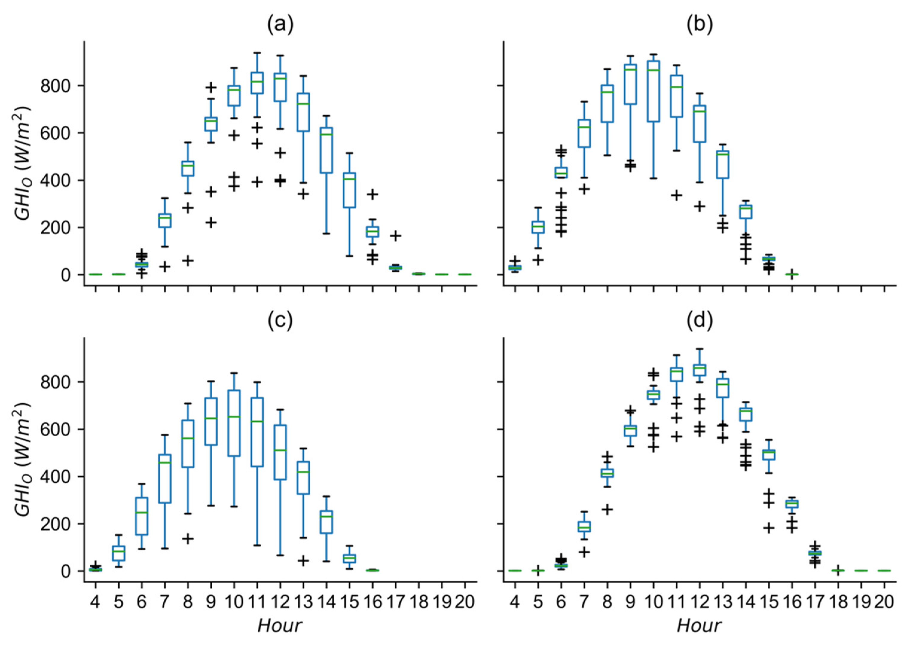
Figure 2 shows the hourly variation of observed GHI for the benchmarking period. All locations show a clear diurnal cycle. All sites in Queensland (Figure 2a,b,d) show a large number of outliers in comparison to Victoria (Figure 2c), which shows lower mean values. Note, Queensland has a tropical climate with greater variability in clouds with several outliers, whereas as Victoria has lower mean GHI with broader distributions. Although the sites are located in regions affected by slightly different meteorological conditions, it is clear that challenges exist in predicting GHI at short time scales of up to an hour.
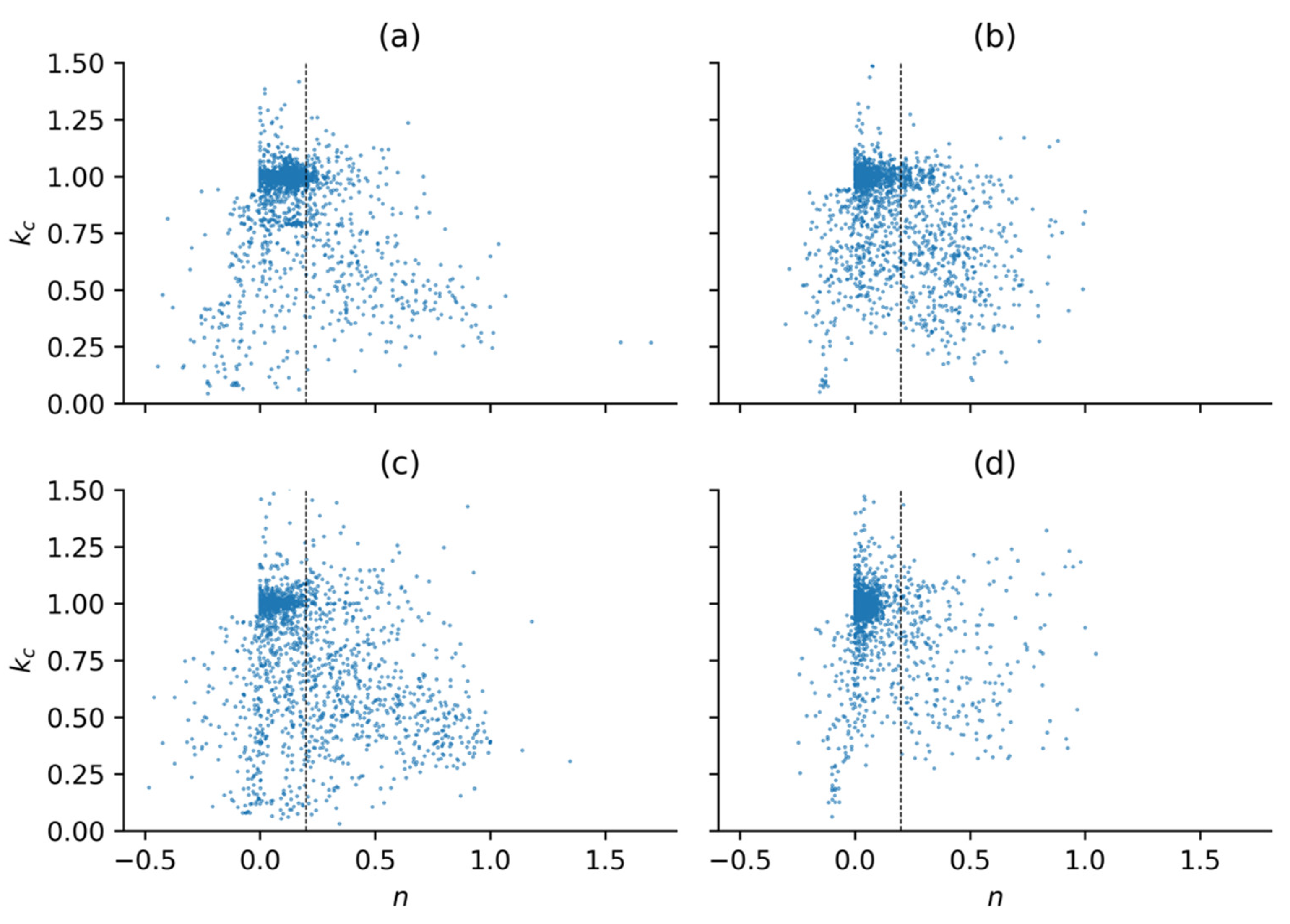
The relationship between the clear sky index () and cloud index () was derived for SIFM. Figure 3 shows the relationships for all the sites investigated in this study. The clear sky index and cloud index show unique characteristics at all sites. A larger cluster of scatter points exist near for , however the cluster grows especially in the space until beyond which a linear decline can be inferred.
Clearly, the relationship observed in Figure 3 can be approximated using piecewise linear functions with separations at using Equation (3). A first order polynomial fit (linear regression) was used to derive the coefficients. The coefficients derived to relate clear sky index () and cloud index () when is listed in Table 3.
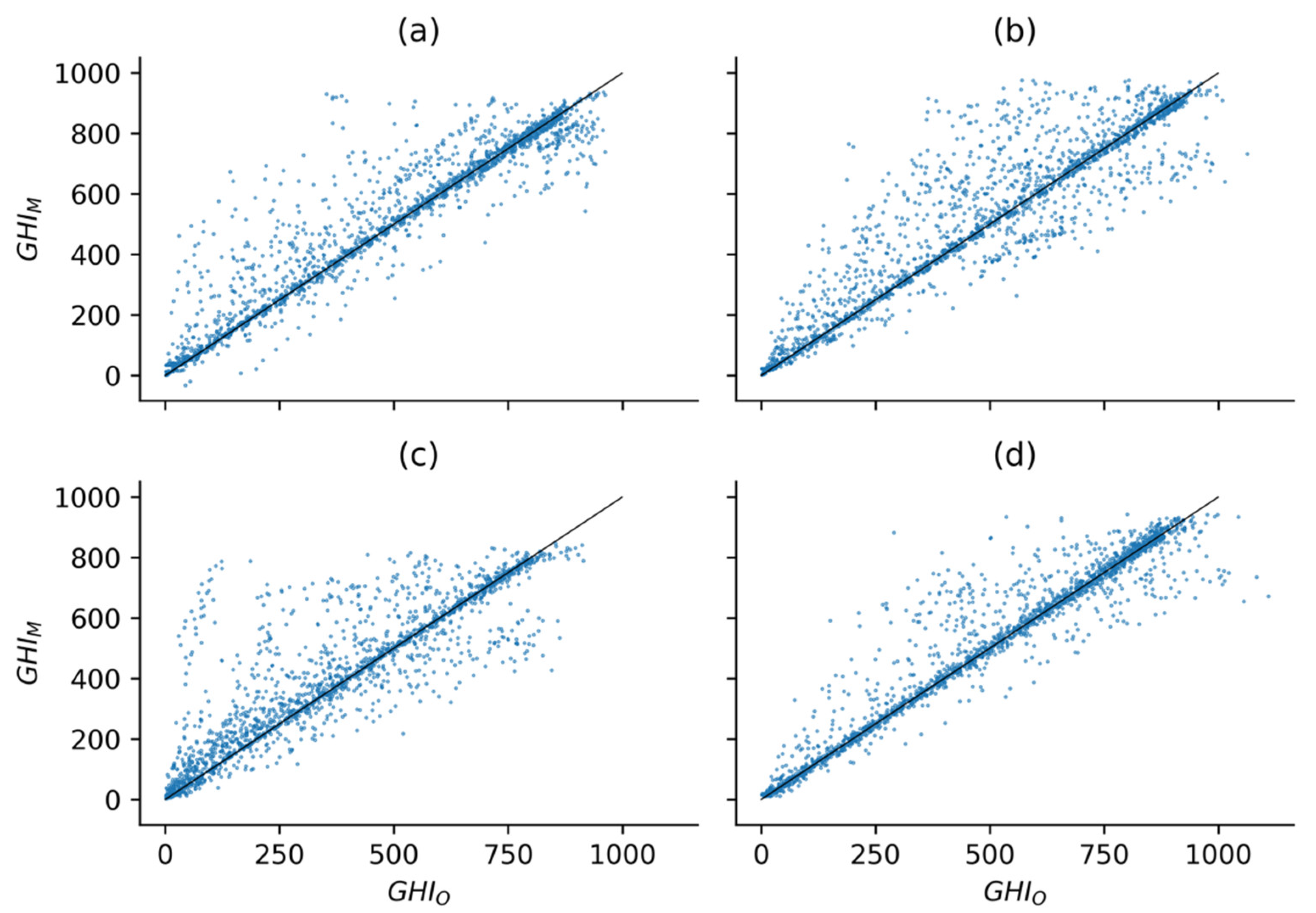
The fitting functions for individual sites was used to model irradiance () with coefficients listed in Table 3. Figure 4 demonstrates the applicability of using cloud index in approximating the clear sky index for the calculation of model irradiance from the clear sky model ():
The error metrics from comparison of modelled and observed GHI at all the sites investigated are shown in Table 4. The modelled and observed GHI closely follow each other at all sites with R2 > 0.7. The GHI values were mostly overestimated by the model in comparison to the observations during the benchmarking period (MBE > 0 Wm−2). All sites showed errors (RMSE < 119 Wm−2, nRMSE < 33%) with QLD-C performing the best. Note, Queensland has a hot to humid subtropical climate whereas Victoria has a cold semi-arid climate. Likewise, QLD-C is more inland than other sites and is less susceptible to oceanic meteorological conditions, such as sea breezes. Several authors also report similar magnitude of errors for all-sky conditions satellite derived GHI related to arid and temperate climates [49,55,56].
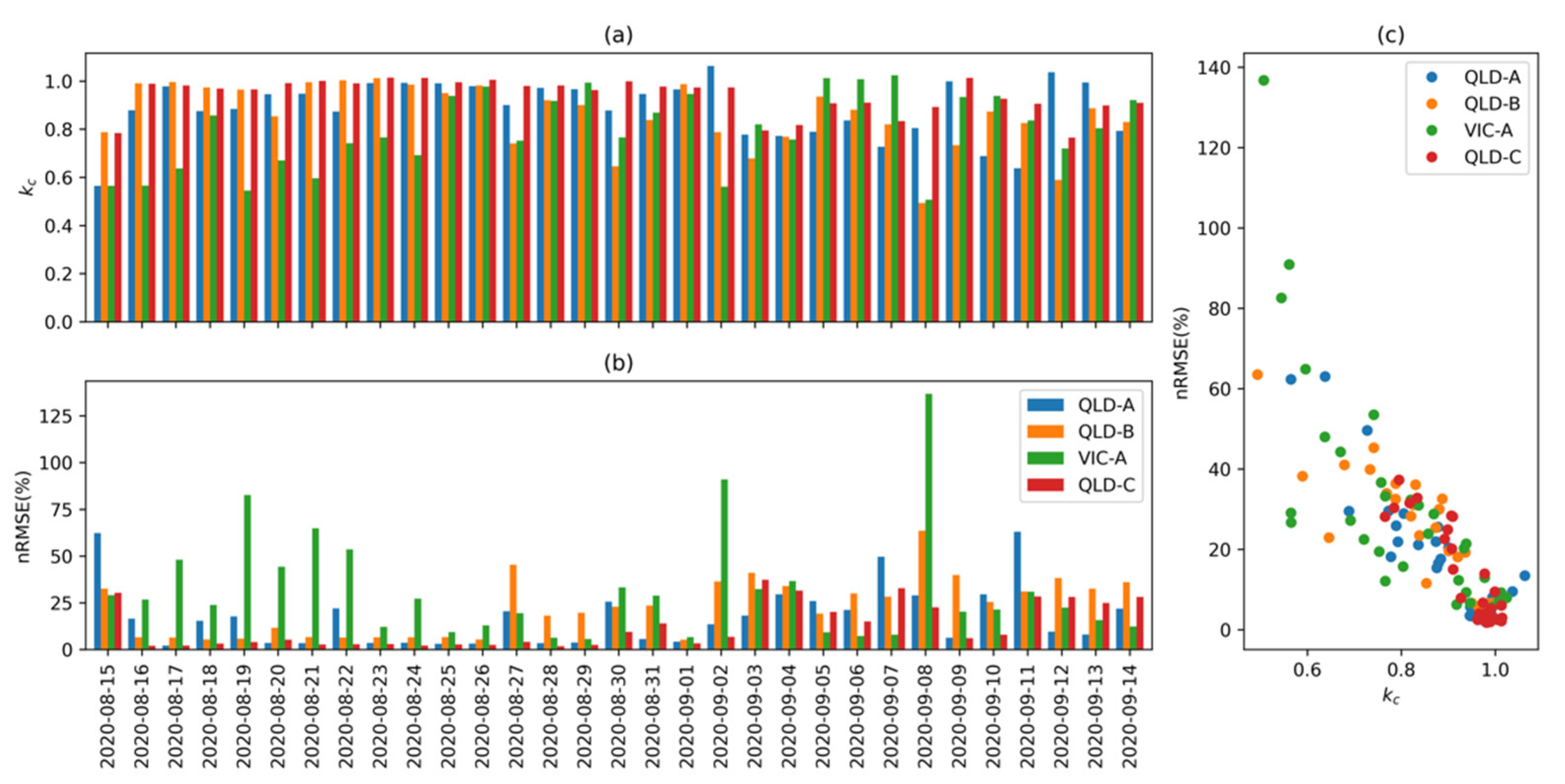
The errors reported in Table 4 included all-sky conditions. Note, each site experiences a different degree of cloudiness influencing these errors. The daily clear sky index and nRMSE related to the calculation of model irradiance () is shown in Figure 5.
The daily variations of clear sky index and nRMSE show errors increase rapidly as cloudiness increases. Furthermore, it is evident that QLD-C performs better due to more clear days in comparison to VIC-A, where cloudy days dominate. It is also evident that all Queensland sites start with more clear days late in the winter and as the season transitions into spring and the temperature warms up, more cloudy days develop resulting in increase in errors.
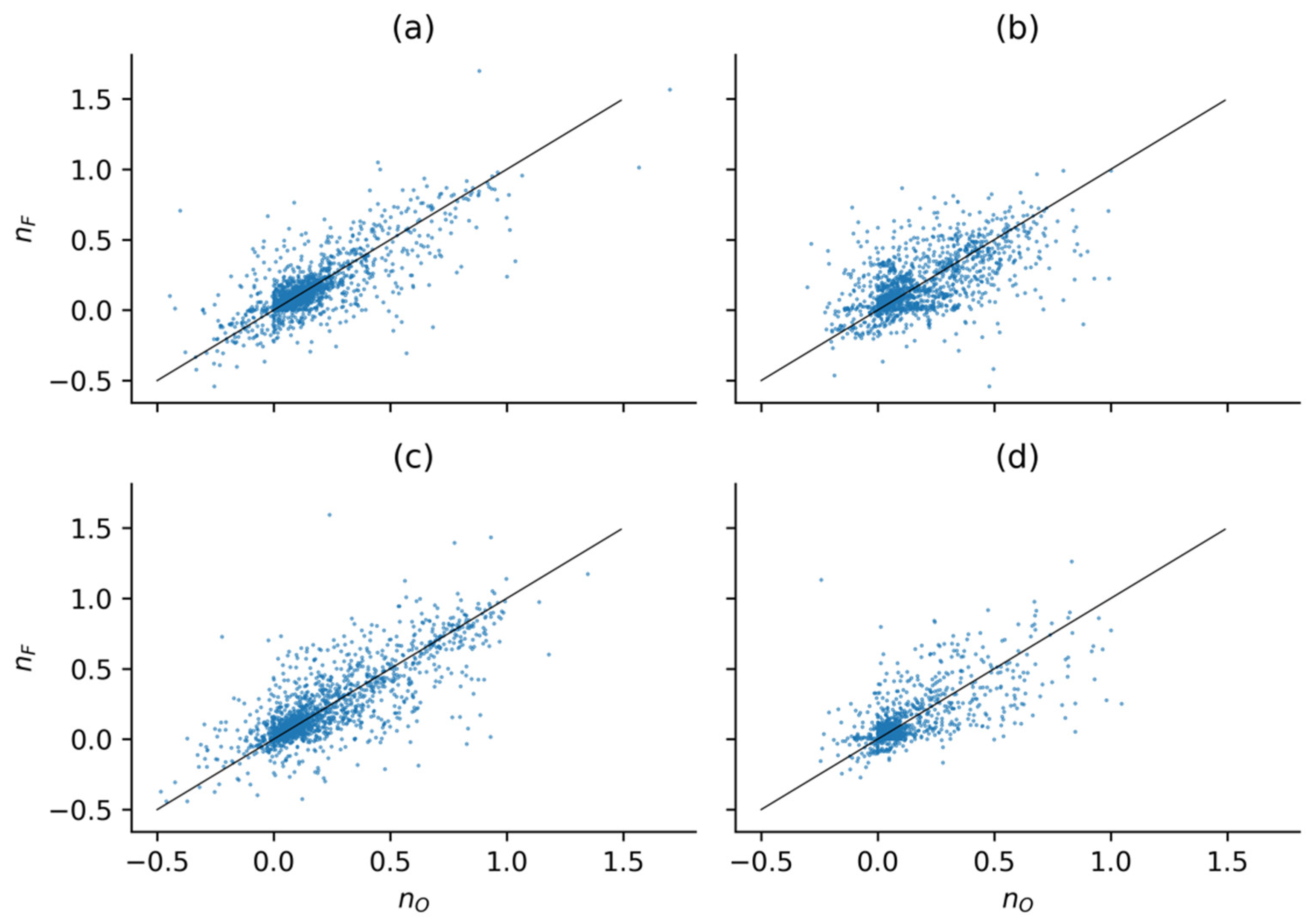
Another critical component of SIFM is image processing for the calculation of CMVs. The observed and predicted cloud index after advection at 5 min using two consecutive satellite images were used to test CMVs for the benchmark period (shown in Figure 6).
The error metrics related to cloud index advected using derived CMVs when compared to observed cloud index is shown in Table 5.
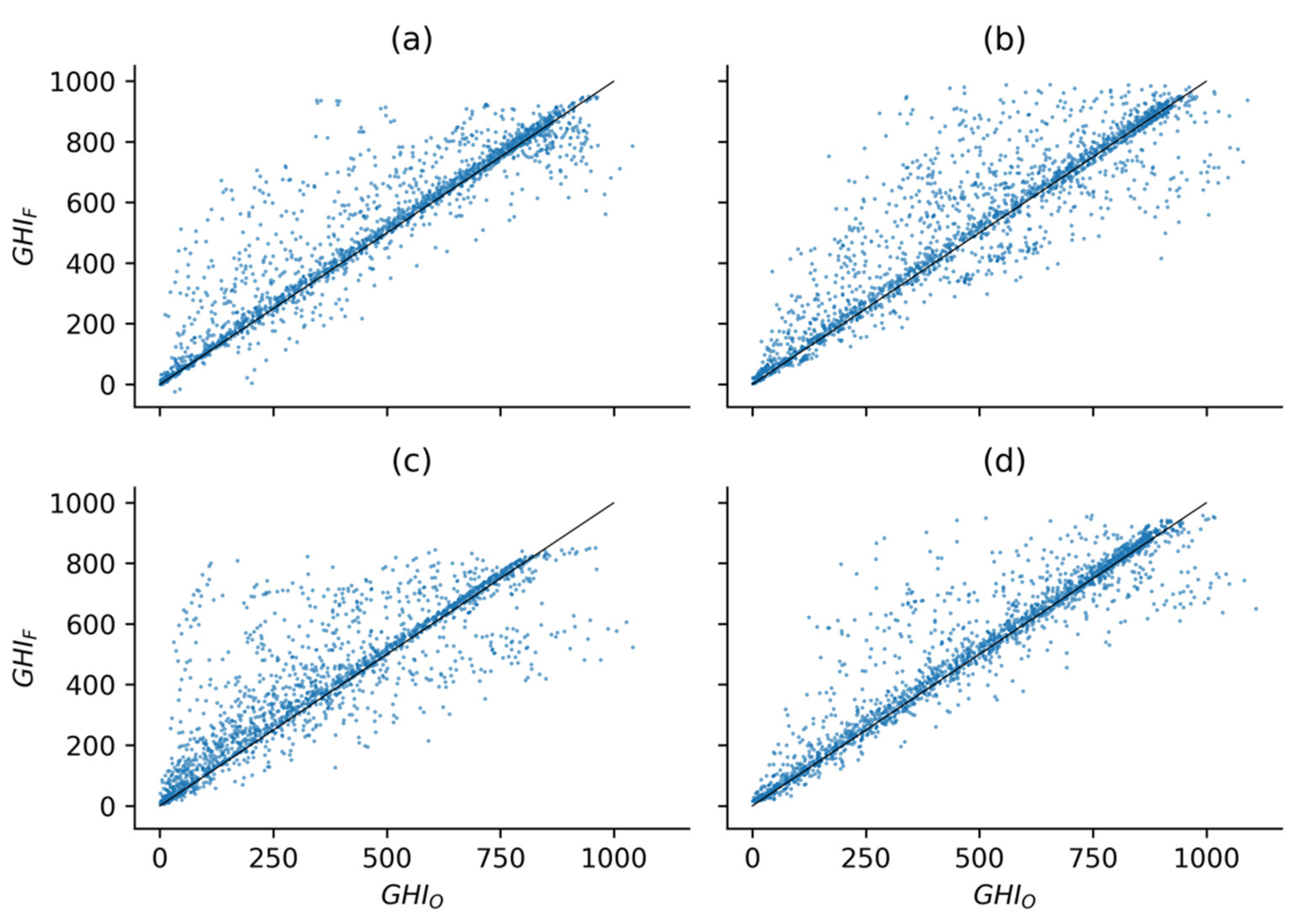
All sites show high residuals, but the forecasted cloud index follows the observed with modest R2, especially for QLD-A and VIC-A. The RMSE and MBE does not change much. A better way of looking at the accuracy of CMVs were to calculate the predicted GHI. Thus, all the predicted clear sky GHI were scaled by the clear-sky index corresponding to the predicted cloud index produced from the advection of cloud motion vectors. The predicted GHI (ensemble mean from all clear sky models) comparison with observations is shown in Figure 7.
The error metrics for predicted (ensemble mean) and observed GHI at a forecast horizon of 5 min is outlined in Table 6.
A number of compensating errors during the conversion of cloud index to clear sky index and the calculation of ensemble mean from clear sky models improve the predicted GHI. It is evident that all sites demonstrate high goodness of fits (R2 > 0.7). The predicted GHI is overestimated at all sites by as much as 79 Wm−2. The errors RMSE and nRMSE at all sites were <138 Wm−2 and 38%, respectively, with QLD-C performing the best.
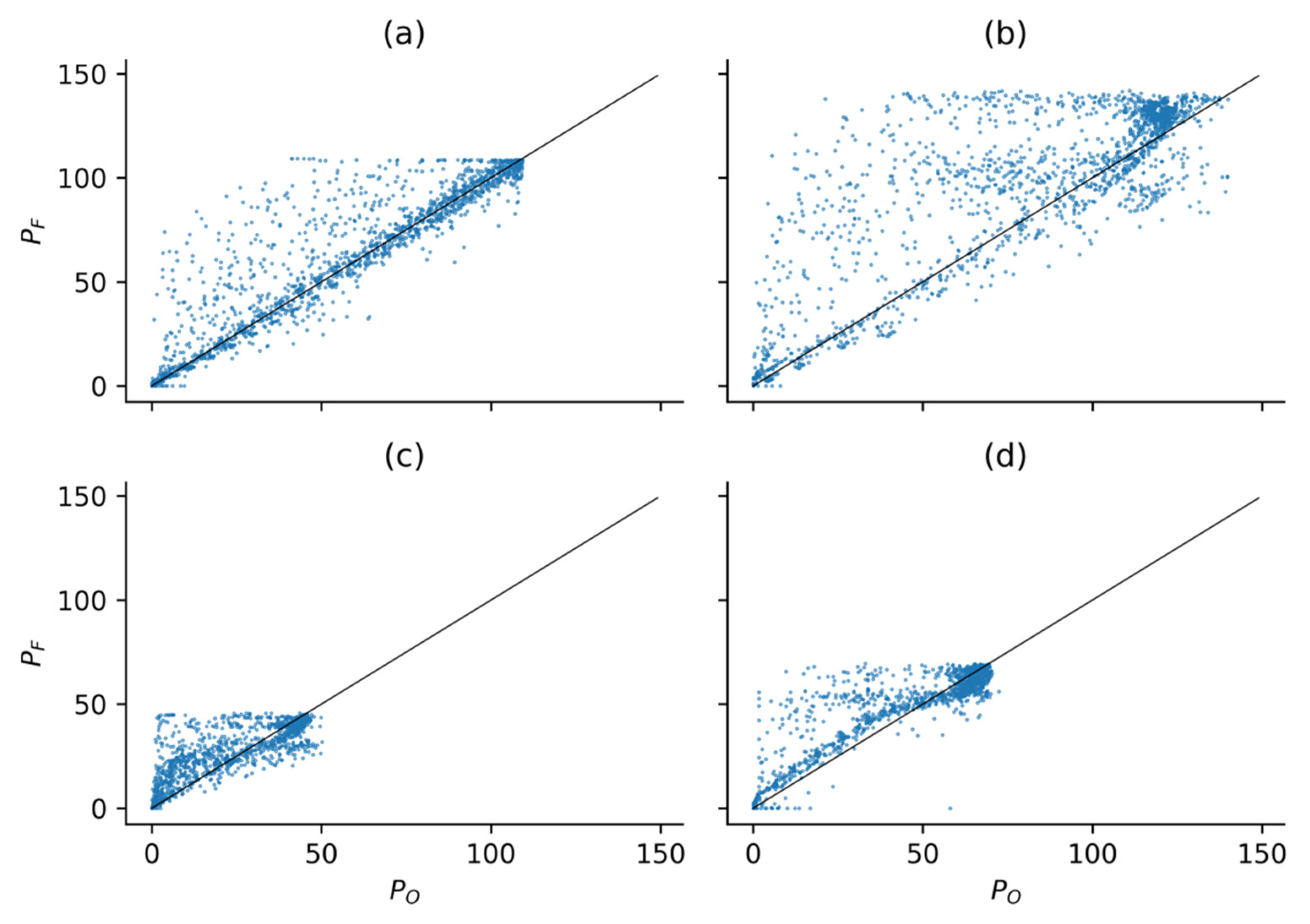
Similarly, the GHI ensemble was converted to power using the power conversion model trained at each site. The predicted power (ensemble mean) comparison with power produced is shown in Figure 8. Similarly, the error metrics for predicted (ensemble mean) and observed power at a forecast horizon of 5 min is also outlined in Table 7.
The conversion of GHI to power forecasts introduces additional errors. Nonetheless, the model closely follows observations at all sites with R2 > 0.6. The generators overestimate forecast power at all sites from 6–19 MW. Due to different capacity of generators, the RMSE cannot be directly compared at each site, but the nRMSE shows Queensland sites performed better (nRMSE < 34%) than the Victoria site.
3.2. Live Predictions
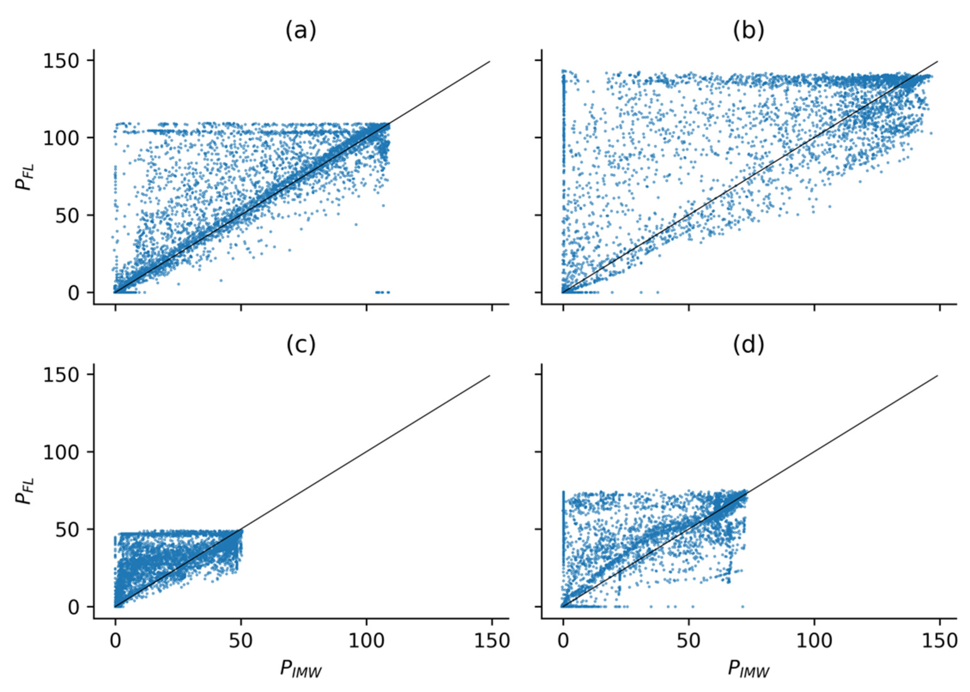
SIFM was tested with live predictions in the market. The forecast horizon was dependent on the latest satellite image available to the scheduled time for dispatch. The predicted power (ensemble mean) comparison with power produced for live predictions (denoted as initalmw) is shown in Figure 9. Likewise, the error metrics for predicted (ensemble mean) and observed power for live predictions are also presented in Table 8.
Generally, live predictions were dependent on the forecast horizons due to the times at which images were archived. Overall, real time predictions were poorer than benchmark predictions due to varying forecasts horizons; however, this was expected. Nonetheless, live predictions functioned in close range with the benchmark period with a 5-min forecast horizon, except for QLD-C.
3.3. Evaluations with Persistence
Comparisons of SIFM with a simple persistence model demonstrates the suitability of SIFM forecasts at short-time intervals. Evaluation metrics such as those reported in Table 8 do not show much difference when comparing SIFM and persistence forecasts to observations. This was expected since CMV based predictions of solar irradiance do not beat persistence at very short-time scales. Nonetheless, we illustrate the forecast skill of SIFM in comparison to simple persistence based on the percentage of samples where the forecasts were within ±1% (err < 1%), ±5% (err < 5%) and ±10% (err < 10%) of the observed for the benchmarking and live predictions in Table 9.
Overall, SIFM beats persistence in capturing greater percentage of good predictions (err < 1%, err < 5% and err < 10%) for GHI in the benchmarking period for all sites. Likewise, SIFM demonstrates greater success than simple persistence in generating predictions with err < 10% for nearly all sites in GHI and power predictions for the benchmarking and live period. Clearly, SIFM produces forecasts (err < 1%, err < 5% and err < 10%) which degrades in quality from GHI to power predictions in the benchmarking period suggesting strong dependence of the PCM. Likewise, SIFM power predictions show lower percentage of good predictions during the live predictions in comparison to the benchmarking period likely due to the different period of study. Moreover, SIFM predictions at Queensland sites capture greater percentage of good predictions (err < 1%, err < 5% and err < 10%) than Victoria, however QLD-A was the only site where SIFM fully beats persistence in GHI and Power predictions for the benchmarking and live period.
Additionally, aggregating the percentage of good predictions (err < 1%, err < 5% and err < 10%) by days demonstrates the daily SIFM skill in comparison to simple persistence forecasts. The percentage of days in the benchmarking and live period where SIFM beats the performance of simple persistence model is shown in Table 10.
Interestingly, SIFM outperforms persistence > 50% of the days in the benchmarking and live period with err < 10% for all sites, except VIC-A for power predictions in the benchmarking period. Note, live prediction period differs from the benchmarking period with forecasts horizons at times of 20–25 min. SIFM outperforms persistence on greater percentage of days during live power predictions in comparison to power predictions from the benchmarking period for all sites. This was expected since CMV based predictions of solar irradiance and power beat persistence at greater forecasts horizons.
4. Discussion
Errors in short-term irradiance forecasts using the advection of derived GHI with CMVs depend more on the quality of derived GHI than the CMVs. All-sky (both clear and cloudy cases) GHI produced using SIFM at four sites produced a nRMSE of 16–33%. Previous studies deriving all-sky GHI using satellite images have also produced similar magnitude of errors. Recently, Kamath and Srinivasan [49] produced GHI using INSAT-3D over India with nRMSE ranging from 18–35% when compared to ground observations for arid, tropical and temperate regions. Similarly, Yang and Bright [55] also compared satellite derived GHI with 57 Baseline Solar Radiation Network (BSRN) stations, which produced nRMSE ranging from 13–30%. Likewise, Bright [56] also showed that Solcast-derived GHI compared at 48 BSRN stations produced nRMSE ranging from 6–44%. SIFM produces GHI errors comparable to other satellite-derived products, however the key source of error in producing GHI using SIFM stems from the calculation of the cloud index and clear sky index. While cloud index calculation can be contaminated by surface reflectance [56] and cloud shadows [12], clear sky models used for the calculation of clear sky index also produces errors [57]. The latter errors can be bias corrected for based on the consistency of errors produced on clear days, however errors in cloud index requires constant injection of monthly datasets with equal proportion of clear and cloudy days that sample surface reflections and cloud shadows.
On the contrary, CMV derivations in SIFM were robust due to the consistent development of the optical flow techniques applied over the satellite images. Notable errors from CMVs only occurred when assumptions used in optical flow techniques were violated due to changes in contrast in satellite imagery with the rapidly developing cumulus congestus clouds. These challenges are not new in deriving CMVs and has been often discussed in the past literature [50]. Likewise, CMV errors can be exacerbated due to increased forecast horizons where cloud morphology changes extensively, especially in a real-time environment affected by latency in acquiring images from the remote data centers. At times, SIFM satellite latency varied from 15–25 min which also added to errors in power predictions in real-time. However, greater errors in SIFM were generated from the power conversion model due to added complexity and training dataset used at different sites with separate module parameters and losses from soiling, wiring and degradations. Notably, SIFM errors resulting from GHI estimates were amplified after power conversion due to the interaction of errors resulting from the two procedures as demonstrated in the benchmarking period of the study.
Although studies related to satellite-derived power predictions are limited, GHI predictions from satellite imagery are numerous, which could be compared to SIFM predictions of GHI in the benchmarking period. SIFM produced errors in nRMSE of 19–35% for 5-min forecasts. Recently, Yang, et al. [27] produced errors in nRMSE of 27% for 30-min GHI forecasts from FengYung-4 geostationary satellite over China. Later, a similar study showed errors in nRMSE of 19–22% for 15-min GHI forecasts [28]. Likewise, Kallio-Myers, et al. [22] demonstrated errors in nRMSE of 17–34% for 15-min GHI forecasts from MSG satellite over Finland. Evidently, for forecast horizons less than 30 min, nearly all studies report similar performance metrics in comparison to SIFM forecasts of GHI beating smart persistence predictions on most occasions, especially at forecasts horizons beyond 15 min.
Moreover, benchmarking performance with smart persistence model is ideal but not often conclusive for skill due to unrealistic prediction of ramps [22]. SIFM introduced more robust comparisons with the percentage of samples where the forecasts were within ±1% (err < 1%), ±5% (err < 5%) and ±10% (err < 10%) of the observed, which was more sensitive to the magnitude of errors. Thus, SIFM outperformed persistence on >50% of the days in the benchmarking and live period with err < 10% for all sites, which demonstrates the application of SIFM in an operational market.
5. Conclusions
This paper evaluates the performance of short-term power forecasts produced from the Satellite Irradiance Forecasting Model (SIFM) using near real-time Himawari-8 satellite images at four solar power farms located in Australia. The downwelling solar irradiance was converted to power forecasts using a power conversion model. SIFM was initially tested with at least one month of data for benchmarking at 5-min forecast horizon and later for operational phases with 15 to 25-min forecast horizon including satellite latency. For the benchmarking period, GHI forecasts produced errors with nRMSE ranging from 19–35% for 5-min forecasts beating persistence at all sites with almost 44–63% of predicted times or 61–84% of days in the period where errors were less than 10%. The model performed better in capturing GHI (especially on clear days), however conversion to power forecasts amplified errors. Power forecasts showcased errors in nRMSE of 24–43% for 5-min forecasts with 43–60% of predicted times or 52–87% of days in the period where errors were less than 10%, beating persistence except for the site in Victoria. During the live demonstration phase with a different period and forecasting horizon, SIFM outperformed persistence with errors less than 10% on 54–91% of days.
SIFM identified several challenges and possibilities of improvements in the future associated with errors resulting from the calculation of cloud index (cloud shadows and surface reflectance), clear sky index (clear sky model related biases), CMVs (cloud contrasts and intensity) and PCM (power conversion assumptions related to soiling, degradations, shading and module components). Notably, the development and movement of clouds are different at each location, including the surface reflectance. SIFM is very sensitive to the darkest and brightest pixels, which indirectly suggests frequent training of the model to derive the fitting functions using the clear sky index and the cloud index is required for live operations. Note, each of the site’s performance has not been weighted by equal number of clear and cloudy days, thus the performance at each site cannot be directly compared. Moreover, the performance of GHI and power predictions are not the same at each site, highlighting issues in deriving GHI and then converting to power using a separate trained power conversion model may compound errors. Nonetheless, SIFM compares well with other models tested outside Australia for GHI predictions and shows promising results for power predictions under live operations.
Author Contributions
Conceptualisation, A.A.P. and M.K.; methodology, A.A.P.; software, A.A.P.; validation, A.A.P. and M.K.; formal analysis, A.A.P.; investigation, A.A.P.; resources, M.K.; data curation, A.A.P.; writing—original draft preparation, A.A.P.; writing—review and editing, A.A.P. and M.K.; visualization, A.A.P.; supervision, M.K.; project administration, M.K.; funding acquisition, A.A.P. and M.K. Both authors have read and agreed to the published version of the manuscript.
Funding
This research was funded by the Australian Renewable Energy Agency (ARENA) for the project Solar Power Ensemble Forecaster (grant no. RG181399).
Acknowledgments
We sincerely acknowledge Ben Duck for developing the Power Conversion Model used in this study. We also thank Sam West, Matt Amos and Sebastian Consani for helpful discussions and installation of SIFM for testing on the cloud services.
Conflicts of Interest
The authors declare no conflict of interest.
Appendix A
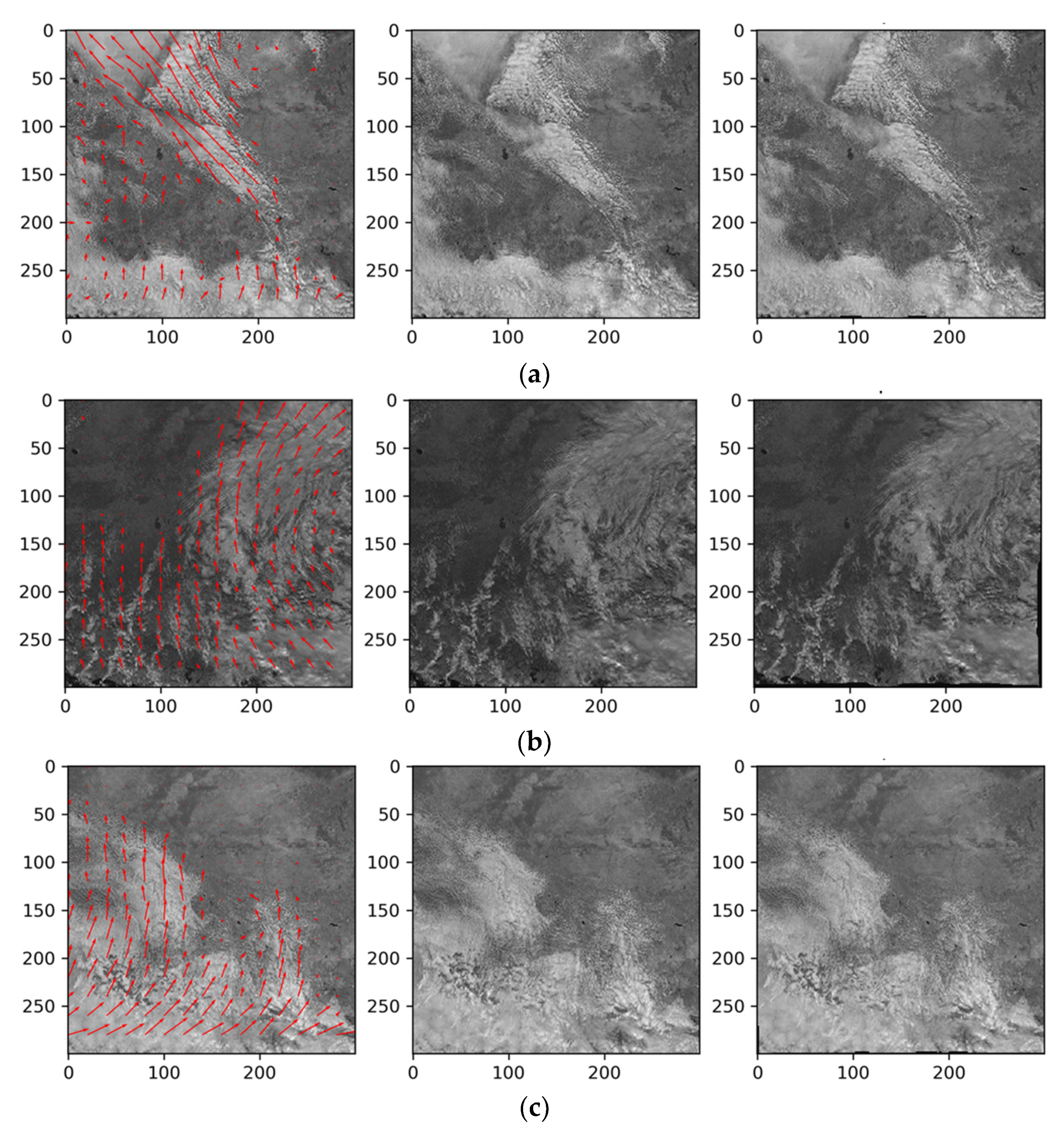
The CMVs derived using optical flow techniques are demonstrated in Figure A1 for satellite images selected in June 2019 during noon for the site in Victoria. The displacement vectors at each cloud index (pixel) are calculated using two consecutive images, which is then extrapolated using the forecast horizon to generate the advected pixel. CMVs are derived properly when contrast in images is high with cloud morphology consistent in time. Figure A1a shows brighter and thicker low-level scattered clouds advected towards the northwest, which matches with the true and predicted imagery.
Figure A1.
CMVs derived using optical flow techniques on (a) 1 June 2019, (b) 3 June 2019 and (c) 5 June 2019 with (left) the original image at noon with displacement vectors, (centre) true satellite image after 10 min from noon and (right) predicted image with a forecast horizon of 10 min using the displacement vectors derived from CMVs.

Similarly, Figure A1b shows organized clouds advected by a frontal circulation with clockwise rotational motion towards the west also matching with the true and predicted imagery. Likewise, Figure A1c shows low-level aggregated clouds advected towards the north closely matching the true and predicted imagery. Note, the startling difference in surface reflectance shown with darker patches in cloud free regions of Figure A1b as compared to Figure A1a,c with contamination from thin clouds over underlying surface.
References
- International Renewable Energy Agency. Renewable Capacity Highlights: 31 March 2021; International Renewable Energy Agency: Abu Dhabi, United Arab Emirates, 2021; p. 3. Available online: https://www.irena.org/publications/2021/March/Renewable-Capacity-Statistics-2021 (accessed on 10 June 2021).
- Department of Industry Science Energy and Resources. Australian Energy Update; Australian Energy Statistics: Canberra, ACT, Australia, 2020. Available online: https://www.energy.gov.au/publications/australian-energy-update-2020 (accessed on 12 June 2021).
- Prăvălie, R.; Patriche, C.; Bandoc, G. Spatial assessment of solar energy potential at global scale. A geographical approach. J. Clean. Prod. 2019, 209, 692–721. [Google Scholar] [CrossRef]
- Prasad, A.A.; Taylor, R.A.; Kay, M. Assessment of direct normal irradiance and cloud connections using satellite data over Australia. Appl. Energy 2015, 143, 301–311. [Google Scholar] [CrossRef]
- Prasad, A.A.; Taylor, R.A.; Kay, M. Assessment of solar and wind resource synergy in Australia. Appl. Energy 2017, 190, 354–367. [Google Scholar] [CrossRef]
- Yin, J.; Molini, A.; Porporato, A. Impacts of solar intermittency on future photovoltaic reliability. Nat. Commun. 2020, 11, 4781. [Google Scholar] [CrossRef] [PubMed]
- Bevrani, H.; Ghosh, A.; Ledwich, G. Renewable energy sources and frequency regulation: Survey and new perspectives. IET Renew. Power Gener. 2010, 4, 438–457. [Google Scholar] [CrossRef] [Green Version]
- Stringer, N.; Haghdadi, N.; Bruce, A.; MacGill, I. Fair consumer outcomes in the balance: Data driven analysis of distributed PV curtailment. Renew. Energy 2021, 173, 972–986. [Google Scholar] [CrossRef]
- Sharma, V.; Aziz, S.M.; Haque, M.H.; Kauschke, T. Effects of high solar photovoltaic penetration on distribution feeders and the economic impact. Renew. Sustain. Energy Rev. 2020, 131, 110021. [Google Scholar] [CrossRef]
- Prasad, A.A.; Kay, M. Assessment of simulated solar irradiance on days of high intermittency using WRF-solar. Energies 2020, 13, 385. [Google Scholar] [CrossRef] [Green Version]
- Law, E.W.; Prasad, A.A.; Kay, M.; Taylor, R.A. Direct normal irradiance forecasting and its application to concentrated solar thermal output forecasting—A review. Sol. Energy 2014, 108, 287–307. [Google Scholar] [CrossRef]
- Miller, S.D.; Rogers, M.A.; Haynes, J.M.; Sengupta, M.; Heidinger, A.K. Short-term solar irradiance forecasting via satellite/model coupling. Sol. Energy 2018, 168, 102–117. [Google Scholar] [CrossRef]
- Law, E.W.; Kay, M.; Taylor, R.A. Evaluating the benefits of using short-term direct normal irradiance forecasts to operate a concentrated solar thermal plant. Sol. Energy 2016, 140, 93–108. [Google Scholar] [CrossRef]
- Kumar, D.S.; Yagli, G.M.; Kashyap, M.; Srinivasan, D. Solar irradiance resource and forecasting: A comprehensive review. IET Renew. Power Gener. 2020, 14, 1641–1656. [Google Scholar] [CrossRef]
- Yang, D. Ensemble model output statistics as a probabilistic site-adaptation tool for satellite-derived and reanalysis solar irradiance. J. Renew. Sustain. Energy 2020, 12, 016102. [Google Scholar] [CrossRef] [Green Version]
- Mishra, M.; Nayak, J.; Naik, B.; Abraham, A. Deep learning in electrical utility industry: A comprehensive review of a decade of research. Eng. Appl. Artif. Intell. 2020, 96, 104000. [Google Scholar] [CrossRef]
- Mayer, M.J.; Gróf, G. Extensive comparison of physical models for photovoltaic power forecasting. Appl. Energy 2021, 283, 116239. [Google Scholar] [CrossRef]
- Ahmed, R.; Sreeram, V.; Mishra, Y.; Arif, M.D. A review and evaluation of the state-of-the-art in PV solar power forecasting: Techniques and optimization. Renew. Sustain. Energy Rev. 2020, 124, 109792. [Google Scholar] [CrossRef]
- Ahmed, A.; Khalid, M. A review on the selected applications of forecasting models in renewable power systems. Renew. Sustain. Energy Rev. 2019, 100, 9–21. [Google Scholar] [CrossRef]
- Yang, D.; Kleissl, J.; Gueymard, C.A.; Pedro, H.T.C.; Coimbra, C.F.M. History and trends in solar irradiance and PV power forecasting: A preliminary assessment and review using text mining. Sol. Energy 2018, 168, 60–101. [Google Scholar] [CrossRef]
- Wang, P.; van Westrhenen, R.; Meirink, J.F.; van der Veen, S.; Knap, W. Surface solar radiation forecasts by advecting cloud physical properties derived from Meteosat Second Generation observations. Sol. Energy 2019, 177, 47–58. [Google Scholar] [CrossRef]
- Kallio-Myers, V.; Riihelä, A.; Lahtinen, P.; Lindfors, A. Global horizontal irradiance forecast for Finland based on geostationary weather satellite data. Sol. Energy 2020, 198, 68–80. [Google Scholar] [CrossRef]
- Gallucci, D.; Romano, F.; Cersosimo, A.; Cimini, D.; Paola, F.D.; Gentile, S.; Geraldi, E.; Larosa, S.; Nilo, S.T.; Ricciardelli, E.; et al. Nowcasting surface solar irradiance with AMESIS via motion vector fields of MSG-SEVIRI data. Remote Sens. 2018, 10, 845. [Google Scholar] [CrossRef] [Green Version]
- Nonnenmacher, L.; Coimbra, C.F.M. Streamline-based method for intra-day solar forecasting through remote sensing. Sol. Energy 2014, 108, 447–459. [Google Scholar] [CrossRef]
- Kim, C.K.; Kim, H.-G.; Kang, Y.-H.; Yun, C.-Y. Toward Improved solar irradiance forecasts: Comparison of the global horizontal irradiances derived from the COMS satellite imagery over the Korean Peninsula. Pure Appl. Geophys. 2017, 174, 2773–2792. [Google Scholar] [CrossRef]
- Jia, D.; Hua, J.; Wang, L.; Guo, Y.; Guo, H.; Wu, P.; Liu, M.; Yang, L. Estimations of Global Horizontal Irradiance and Direct Normal Irradiance by Using Fengyun-4A Satellite Data in Northern China. Remote Sens. 2021, 13, 790. [Google Scholar] [CrossRef]
- Yang, L.; Gao, X.; Hua, J.; Wu, P.; Li, Z.; Jia, D. Very Short-Term Surface Solar Irradiance Forecasting Based on FengYun-4 Geostationary Satellite. Sensors 2020, 20, 2606. [Google Scholar] [CrossRef]
- Yang, L.; Gao, X.; Li, Z.; Jia, D.; Jiang, J. Nowcasting of surface solar irradiance using FengYun-4 satellite observations over China. Remote Sens. 2019, 11, 1984. [Google Scholar] [CrossRef] [Green Version]
- Qin, Y.; Huang, J.; McVicar, T.R.; West, S.; Khan, M.; Steven, A.D.L. Estimating surface solar irradiance from geostationary Himawari-8 over Australia: A physics-based method with calibration. Sol. Energy 2021, 220, 119–129. [Google Scholar] [CrossRef]
- Kim, M.; Song, H.; Kim, Y. Direct short-term forecast of photovoltaic power through a comparative study between COMS and Himawari-8 meteorological satellite images in a deep neural network. Remote Sens. 2020, 12, 2357. [Google Scholar] [CrossRef]
- Hammer, A.; Heinemann, D.; Lorenz, E.; Lückehe, B. Short-term forecasting of solar radiation: A statistical approach using satellite data. Sol. Energy 1999, 67, 139–150. [Google Scholar] [CrossRef]
- Arbizu-Barrena, C.; Ruiz-Arias, J.A.; Rodríguez-Benítez, F.J.; Pozo-Vázquez, D.; Tovar-Pescador, J. Short-term solar radiation forecasting by advecting and diffusing MSG cloud index. Sol. Energy 2017, 155, 1092–1103. [Google Scholar] [CrossRef]
- Cano, D.; Monget, J.M.; Albuisson, M.; Guillard, H.; Regas, N.; Wald, L. A method for the determination of the global solar-radiation from meteorological satellite data. Sol. Energy 1986, 37, 31–39. [Google Scholar] [CrossRef] [Green Version]
- Rigollier, C.; Lefèvre, M.; Wald, L. The method Heliosat-2 for deriving shortwave solar radiation from satellite images. Sol. Energy 2004, 77, 159–169. [Google Scholar] [CrossRef] [Green Version]
- McCandless, T.; Jiménez, P.A. Examining the potential of a random forest derived cloud mask from GOES-R satellites to improve solar irradiance forecasting. Energies 2020, 13, 1671. [Google Scholar] [CrossRef] [PubMed] [Green Version]
- Yagli, G.M.; Yang, D.; Srinivasan, D. Automatic hourly solar forecasting using machine learning models. Renew. Sustain. Energy Rev. 2019, 105, 487–498. [Google Scholar] [CrossRef]
- Lago, J.; De Brabandere, K.; De Ridder, F.; De Schutter, B. Short-term forecasting of solar irradiance without local telemetry: A generalized model using satellite data. Sol. Energy 2018, 173, 566–577. [Google Scholar] [CrossRef] [Green Version]
- Ayet, A.; Tandeo, P. Nowcasting solar irradiance using an analog method and geostationary satellite images. Sol. Energy 2018, 164, 301–315. [Google Scholar] [CrossRef] [Green Version]
- Aguiar, L.M.; Pereira, B.; Lauret, P.; Díaz, F.; David, M. Combining solar irradiance measurements, satellite-derived data and a numerical weather prediction model to improve intra-day solar forecasting. Renew. Energy 2016, 97, 599–610. [Google Scholar] [CrossRef] [Green Version]
- Aguiar, L.M.; Pereira, B.; David, M.; Díaz, F.; Lauret, P. Use of satellite data to improve solar radiation forecasting with Bayesian Artificial Neural Networks. Sol. Energy 2015, 122, 1309–1324. [Google Scholar] [CrossRef]
- Marquez, R.; Pedro, H.T.C.; Coimbra, C.F.M. Hybrid solar forecasting method uses satellite imaging and ground telemetry as inputs to ANNs. Sol. Energy 2013, 92, 176–188. [Google Scholar] [CrossRef]
- Yang, D.; Li, W.; Yagli, G.M.; Srinivasan, D. Operational solar forecasting for grid integration: Standards, challenges, and outlook. Sol. Energy 2021, 224, 930–937. [Google Scholar] [CrossRef]
- Chen, R.; Wang, J.; Botterud, A.; Sun, H. Wind power providing flexible ramp product. IEEE Trans. Power Syst. 2016, 32, 2049–2061. [Google Scholar] [CrossRef] [Green Version]
- Keeratimahat, K.; Bruce, A.; MacGill, I. Analysis of short-term operational forecast deviations and controllability of utility-scale photovoltaic plants. Renew. Energy 2021, 167, 343–358. [Google Scholar] [CrossRef]
- Yang, D.; Wu, E.; Kleissl, J. Operational solar forecasting for the real-time market. Int. J. Forecast. 2019, 35, 1499–1519. [Google Scholar] [CrossRef]
- El hendouzi, A.; Bourouhou, A. Solar Photovoltaic Power Forecasting. J. Electr. Comput. Eng. 2020, 2020, 1–21. [Google Scholar] [CrossRef]
- Bessho, K.; Date, K.; Hayashi, M.; Ikeda, A.; Imai, T.; Inoue, H.; Kumagai, Y.; Miyakawa, T.; Murata, H.; Ohno, T.; et al. An introduction to Himawari-8/9—Japan’s new-generation geostationary meteorological satellites. J. Meteorol. Soc. Jap. 2016, 94, 151–183. [Google Scholar] [CrossRef] [Green Version]
- Hammer, A.; Heinemann, D.; Hoyer, C.; Kuhlemann, R.; Lorenz, E.; Müller, R.; Beyer, H.G. Solar energy assessment using remote sensing technologies. Remote Sens. Environ. 2003, 86, 423–432. [Google Scholar] [CrossRef]
- Kamath, H.G.; Srinivasan, J. Validation of global irradiance derived from INSAT-3D over India. Sol. Energy 2020, 202, 45–54. [Google Scholar] [CrossRef]
- Urbich, I.; Bendix, J.; Müller, R. A novel approach for the short-term forecast of the effective cloud albedo. Remote Sens. 2018, 10, 955. [Google Scholar] [CrossRef] [Green Version]
- Farnebäck, G. Two-frame motion estimation based on polynomial expansion. Lect. Notes Comput. Sci. 2003, 2749, 363–370. [Google Scholar]
- Ineichen, P. A broadband simplified version of the Solis clear sky model. Sol. Energy 2008, 82, 758–762. [Google Scholar] [CrossRef] [Green Version]
- Ineichen, P.; Perez, R. A new airmass independent formulation for the Linke turbidity coefficient. Sol. Energy 2002, 73, 151–157. [Google Scholar] [CrossRef] [Green Version]
- André, M.; Perez, R.; Soubdhan, T.; Schlemmer, J.; Calif, R.; Monjoly, S. Preliminary assessment of two spatio-temporal forecasting technics for hourly satellite-derived irradiance in a complex meteorological context. Sol. Energy 2019, 177, 703–712. [Google Scholar] [CrossRef]
- Yang, D.; Bright, J.M. Worldwide validation of 8 satellite-derived and reanalysis solar radiation products: A preliminary evaluation and overall metrics for hourly data over 27 years. Sol. Energy 2020, 210, 3–19. [Google Scholar] [CrossRef]
- Bright, J.M. Solcast: Validation of a satellite-derived solar irradiance dataset. Sol. Energy 2019, 189, 435–449. [Google Scholar] [CrossRef]
- Engerer, N.A.; Mills, F.P. Validating nine clear sky radiation models in Australia. Sol. Energy 2015, 120, 9–24. [Google Scholar] [CrossRef]
Figure 1.
Flowchart representing the basic operations of SIFM.

Figure 2.
Hourly variation of observed GHI in the benchmarking period for: (a) QLD-A; (b) QLD-B; (c) VIC-A; (d) QLD-C. Outliers in the distribution are denoted with the “+” symbol.
Figure 2.
Hourly variation of observed GHI in the benchmarking period for: (a) QLD-A; (b) QLD-B; (c) VIC-A; (d) QLD-C. Outliers in the distribution are denoted with the “+” symbol.

Figure 3.
The relationship between the clear sky index () and cloud index () in the benchmarking period for: (a) QLD-A; (b) QLD-B; (c) VIC-A; (d) QLD-C. A vertical black dashed line at separates the relationship between and .
Figure 3.
The relationship between the clear sky index () and cloud index () in the benchmarking period for: (a) QLD-A; (b) QLD-B; (c) VIC-A; (d) QLD-C. A vertical black dashed line at separates the relationship between and .

Figure 4.
Modelled versus observed GHI in the benchmarking period for: (a) QLD-A; (b) QLD-B; (c) VIC-A; (d) QLD-C. The reference line y = x is shown in black.
Figure 4.
Modelled versus observed GHI in the benchmarking period for: (a) QLD-A; (b) QLD-B; (c) VIC-A; (d) QLD-C. The reference line y = x is shown in black.

Figure 5.
Daily evaluations of modelled GHI and cloudiness in the benchmarking period for: (a) mean clear sky index; (b) nRMSE; (c) relationship between daily clearness and errors in deriving GHI.
Figure 5.
Daily evaluations of modelled GHI and cloudiness in the benchmarking period for: (a) mean clear sky index; (b) nRMSE; (c) relationship between daily clearness and errors in deriving GHI.

Figure 6.
Forecasted cloud index at 5 min compared to observed in the benchmarking period for: (a) QLD-A; (b) QLD-B; (c) VIC-A; (d) QLD-C. The reference line y = x is shown in black.
Figure 6.
Forecasted cloud index at 5 min compared to observed in the benchmarking period for: (a) QLD-A; (b) QLD-B; (c) VIC-A; (d) QLD-C. The reference line y = x is shown in black.

Figure 7.
Forecasted GHI (ensemble mean) at 5 min compared to observed GHI in the benchmarking period for: (a) QLD-A; (b) QLD-B; (c) VIC-A; (d) QLD-C. The reference line y = x is shown in black.
Figure 7.
Forecasted GHI (ensemble mean) at 5 min compared to observed GHI in the benchmarking period for: (a) QLD-A; (b) QLD-B; (c) VIC-A; (d) QLD-C. The reference line y = x is shown in black.

Figure 8.
Forecasted power (ensemble mean) at 5 min compared to observed power in the benchmarking period for: (a) QLD-A; (b) QLD-B; (c) VIC-A; (d) QLD-C. The reference line y = x is shown in black.
Figure 8.
Forecasted power (ensemble mean) at 5 min compared to observed power in the benchmarking period for: (a) QLD-A; (b) QLD-B; (c) VIC-A; (d) QLD-C. The reference line y = x is shown in black.

Figure 9.
Forecasted power (ensemble mean) compared to observed power in the live period for: (a) QLD-A; (b) QLD-B; (c) VIC-A; (d) QLD-C. The reference line y = x is shown in black.
Figure 9.
Forecasted power (ensemble mean) compared to observed power in the live period for: (a) QLD-A; (b) QLD-B; (c) VIC-A; (d) QLD-C. The reference line y = x is shown in black.


Table 1.
Summary of solar farms.
| Sites 1 | Name | Capacity (MW) | Internet | Climate |
|---|---|---|---|---|
| Queensland A | QLD-A | 110 | 4G | Humid subtropical |
| Queensland B | QLD-B | 150 | Site | Hot and humid |
| Queensland C | QLD-C | 50 | Site | Humid subtropical |
| Victoria A | VIC-A | 72 | 4G | Cold semi-arid |
1 Solar farm names have been suppressed due to non-disclosure agreement.
Table 2.
Clear sky models used in generating the ensemble product.
| Ensemble | Clear Sky Model | Parameters |
|---|---|---|
| A | Ineichen | Climatological Turbidity |
| B | Ineichen | 1.1 × Climatological Turbidity |
| C | Ineichen | 0.9 × Climatological Turbidity |
| D | Haurwitz | Apparent Zenith Angle |
| E | Simplified Solis | Climatological Aerosol Optical Depth |
| F | Simplified Solis | 1.1 × Climatological Aerosol Optical Depth |
| G | Simplified Solis | 0.9 × Climatological Aerosol Optical Depth |
Table 3.
Coefficients relating cloud index to clear sky index.
| Sites | Name | a | b |
|---|---|---|---|
| Queensland A | QLD-A | 0.32877541 | 0.75064906 |
| Queensland B | QLD-B | 0.40395545 | 0.47190695 |
| Queensland C | QLD-C | 0.13397656 | 0.70901523 |
| Victoria A | VIC-A | 0.40674933 | 0.447415 |
Note, the relationship is static for the benchmark calculations but for real-time analysis, this relationship requires a monthly update to account for seasonal surface albedo changes affecting the calculation of the apparent ground albedo ().
Table 4.
Error metrics for modelled and observed GHI in the benchmarking period.
| Site Name | RMSE (Wm−2) | MBE (Wm−2) | MAE (Wm−2) | R2 |
|---|---|---|---|---|
| QLD-A | 92.49 (20%) | 21.03 | 47.91 | 0.90 |
| QLD-B | 113.58 (24%) | 26.41 | 65.52 | 0.84 |
| QLD-C | 78.08 (16%) | 12.66 | 38.27 | 0.92 |
| VIC-A | 118.58 (33%) | 28.78 | 62.63 | 0.77 |
nRMSE are listed in parenthesis.
Table 5.
Error Metrics for predicted cloud index at advection of 5 min.
| Site Name | RMSE | MBE | MAE | R2 |
|---|---|---|---|---|
| QLD-A | 0.13 | 0.07 | −0.0030 | 0.53 |
| QLD-B | 0.15 | 0.09 | 0.0002 | 0.29 |
| QLD-C | 0.11 | 0.06 | 0.0021 | 0.42 |
| VIC-A | 0.15 | 0.09 | 0.0039 | 0.61 |
Table 6.
Error metrics for predicted mean GHI ensemble at advection of 5 min.
| Site Name | RMSE (Wm−2) | MBE (Wm−2) | MAE (Wm−2) | R2 |
|---|---|---|---|---|
| QLD-A | 106.04 (23%) | 55.96 | 32.89 | 0.86 |
| QLD-B | 124.99 (26%) | 73.55 | 35.28 | 0.82 |
| QLD-C | 91.06 (19%) | 47.08 | 22.70 | 0.90 |
| VIC-A | 137.01(38%) | 78.59 | 39.32 | 0.71 |
nRMSE are listed in parenthesis.
Table 7.
Error metrics for predicted mean power ensemble at advection of 5 min.
| Site Name | RMSE (MW) | MBE (MW) | MAE (MW) | R2 |
|---|---|---|---|---|
| QLD-A | 14.14 (24%) | 7.44 | 4.35 | 0.85 |
| QLD-B | 28.75 (34%) | 19.35 | 14.48 | 0.49 |
| QLD-C | 11.09 (24%) | 7.07 | 3.12 | 0.76 |
| VIC-A | 10.05 (43%) | 6.69 | 3.16 | 0.62 |
nRMSE are listed in parenthesis.
Table 8.
Error metrics for predicted mean power ensemble for the live period.
| Site Name | RMSE (MW) | MBE (MW) | MAE (MW) | R2 |
|---|---|---|---|---|
| QLD-A | 18.36 (62%) | 5.38 | 7.66 | 0.77 |
| QLD-B | 40.42 (89%) | 14.92 | 19.40 | 0.48 |
| QLD-C | 23.13 (130%) | 8.47 | 11.37 | 0.23 |
| VIC-A | 10.57 (79%) | 3.76 | 5.42 | 0.63 |
nRMSE are listed in parenthesis.
Table 9.
SIFM skill compared to simple persistence forecasts in the benchmarking and live period.
| Operations | Error | QLD-A (%) | QLD-B (%) | QLD-C (%) | VIC-A (%) |
|---|---|---|---|---|---|
| GHI (Benchmarking) | err < 1% | 16 (8) | 9 (5) | 15 (16) | 10 (3) |
| err < 5% | 49 (33) | 38 (27) | 48 (38) | 33 (23) | |
| err < 10% | 63 (50) | 52 (43) | 63 (53) | 44 (39) | |
| Power (Benchmarking) | err < 1% | 12 (10) | 4 (22) | 8 (27) | 6 (15) |
| err < 5% | 43 (32) | 20 (40) | 31 (43) | 20 (32) | |
| err < 10% | 60 (48) | 43 (47) | 50 (49) | 34 (38) | |
| Power (Live Predictions) | err < 1% | 7 (5) | 2 (10) | 3 (6) | 4 (8) |
| err < 5% | 19 (9) | 14 (15) | 13 (11) | 13 (14) | |
| err < 10% | 26 (16) | 20 (20) | 18 (14) | 18 (18) |
Persistence forecasts are listed in parenthesis.
Table 10.
Percentage of days where SIFM outperforms simple persistence forecasts for the benchmarking and live period.
Table 10.
Percentage of days where SIFM outperforms simple persistence forecasts for the benchmarking and live period.
| Operations | Error | QLD-A (%) | QLD-B (%) | QLD-C (%) | VIC-A (%) |
|---|---|---|---|---|---|
| GHI (Benchmarking) | err < 1% | 48 | 67 | 32 | 58 |
| err < 5% | 74 | 74 | 68 | 77 | |
| err < 10% | 84 | 81 | 81 | 61 | |
| Power (Benchmarking) | err < 1% | 39 | 26 | 10 | 16 |
| err < 5% | 71 | 23 | 13 | 6 | |
| err < 10% | 87 | 52 | 54 | 26 | |
| Power (Live Predictions) | err < 1% | 83 | 26 | 48 | 17 |
| err < 5% | 91 | 51 | 71 | 34 | |
| err < 10% | 91 | 54 | 80 | 54 |
Publisher’s Note: MDPI stays neutral with regard to jurisdictional claims in published maps and institutional affiliations. |
© 2021 by the authors. Licensee MDPI, Basel, Switzerland. This article is an open access article distributed under the terms and conditions of the Creative Commons Attribution (CC BY) license (https://creativecommons.org/licenses/by/4.0/).
Share and Cite
MDPI and ACS Style
Prasad, A.A.; Kay, M. Prediction of Solar Power Using Near-Real Time Satellite Data. Energies 2021, 14, 5865. https://0-doi-org.brum.beds.ac.uk/10.3390/en14185865
AMA Style
Prasad AA, Kay M. Prediction of Solar Power Using Near-Real Time Satellite Data. Energies. 2021; 14(18):5865. https://0-doi-org.brum.beds.ac.uk/10.3390/en14185865
Chicago/Turabian StylePrasad, Abhnil Amtesh, and Merlinde Kay. 2021. "Prediction of Solar Power Using Near-Real Time Satellite Data" Energies 14, no. 18: 5865. https://0-doi-org.brum.beds.ac.uk/10.3390/en14185865
Note that from the first issue of 2016, this journal uses article numbers instead of page numbers. See further details here.