
Forecasting Water Quality Index in Groundwater Using Artificial Neural Network


1
Faculty of Management, Lublin University of Technology, 20-618 Lublin, Poland
2
Faculty of Environmental Engineering, Lublin University of Technology, 20-618 Lublin, Poland
*
Author to whom correspondence should be addressed.
Energies 2021, 14(18), 5875; https://0-doi-org.brum.beds.ac.uk/10.3390/en14185875
Submission received: 14 July 2021
/
Revised: 1 September 2021
/
Accepted: 13 September 2021
/
Published: 16 September 2021
(This article belongs to the Special Issue Economic Analysis and Policies for the Environment, Natural Resources and Energy)
Abstract
:Groundwater quality monitoring in the vicinity of drilling sites is crucial for the protection of water resources. Selected physicochemical parameters of waters were marked in the study. The water was collected from 19 wells located close to a shale gas extraction site. The water quality index was determined from the obtained parameters. A secondary objective of the study was to test the capacity of the artificial neural network (ANN) methods to model the water quality index in groundwater. The number of ANN input parameters was optimized and limited to seven, which was derived using a multiple regression model. Subsequently, using the stepwise regression method, models with ever fewer variables were tested. The best parameters were obtained for a network with five input neurons (electrical conductivity, pH as well as calcium, magnesium and sodium ions), in addition to five neurons in the hidden layer. The results showed that the use of the parameters is a convenient approach to modeling water quality index with satisfactory and appropriate accuracy. Artificial neural network methods exhibited the capacity to predict water quality index at the desirable level of accuracy (RMSE = 0.651258, R = 0.9992 and R2 = 0.9984). Neural network models can thus be used to directly predict the quality of groundwater, particularly in industrial areas. This proposed method, using advanced artificial intelligence, can aid in water treatment and management. The novelty of these studies is the use of the ANN network to forecast WQI groundwater in an area in eastern Poland that was not previously studied—in Lublin.
1. Introduction
Groundwater is one of the key water supply sources for people worldwide. Its quality is an issue of grave importance, as it is directly related to human health [1]. Consumption of contaminated water leads to health problems, as well as increased morbidity and mortality [2].
Industrial activities present a dire threat to the quality of groundwater [3]. The accelerated technological development of our civilization, which is fueled by the energy from crude oil and gas, has contributed to significant pollution of waters with oil derivatives among others [4].
Water quality indices (WQI) facilitate the water quality assessment. In some countries, they have been introduced into legal acts and are often used by the authorities supervising water quality [5]. One of such indicators is the water quality index (WQI), which is an established and one of the most effective tools for assessing water quality [6]. It is a stable, accurate unit of measure that informs about water quality [7]. No single parameter that characterizes the chemical, physical or biological properties of water can adequately express the WQI. WQI is typically assessed by measuring a wide range of parameters (e.g., temperature, pH, electrical conductivity (EC), turbidity, organic matter, metals). The advantage that WQI has over other assessment methods is that it determines the overall state of water quality without performing an individual interpretation of particular parameters [8]. However, computing the WQI may prove both time and effort-intensive, as well as occasionally involve unintended errors, which tend to occur when computing sub-indices. Therefore, mathematical models, especially those based on neural networks, are worth considering as water quality assessment tools [9]. The application of mathematical models for modeling water quality can aid in solving the problems with the management of its quality. Models can simulate the water quality conditions. Such an approach has numerous advantages, including the reduction in cost and time investment in analyses, lower demand for laboratory equipment and apparatus, ability to generate large amounts of synthesized data for analyses, and regeneration of missing data [10]. Mathematical models have the unique capacity for handling information deficit and unavailability of data, in addition to the flexibility with respect to limiting the scope of data for the assessment or prediction of the state of analyzed objects, if necessary.
Currently, an increase in the use of ANNs for predicting the value of the WQI from the applicable water quality parameters can be observed. ANNs constitute an alternative method for understanding and monitoring the quality of groundwater as well as the water in rivers and lakes. They are successfully used as a tool for calculating and predicting the water quality in various bodies of water.
Various studies examining the water quality index were presented. Hatzikos et al. (2008) used neural networks with active neurons as a tool to predict the future (daily) indicators of seawater quality, such as water temperature, pH, dissolved oxygen (DO), and turbidity. Experimental results yielded interesting information on the target variables and algorithm efficiency [11]. Yesilnacar et al. (2008) predicted the nitrate concentration in groundwater using four parameters of temperature, electrical conductivity, groundwater level, and pH as input parameters in the ANN. The model tracked the experimental data very closely (R = 0.93). Hence, with the proposed model application, it is possible to manage groundwater resources in a more cost-effective and easier way [12]. Hore proposed an ANN for predicting WQI the input parameters of which were seasonal and positional variability of wastewater parameters under natural conditions [13]. In turn, the ANN-based model developed by Salman et al. used monthly datasets on turbidity, total hardness, total dissolved solids, and electrical conductivity of the Shatt Al Arab River [14]. The results obtained by Chen et al. indicate that ANN models exhibit very high efficiency in predicting the quality of groundwater, as well as the water in rivers, lakes, and wastewater treatment plants (WWTP) [15].
The issues which may be encountered during ANN implementation include, e.g., inappropriate network structure, selection of an appropriate number of inputs and outputs, as well as the number of cases used for modeling. Correct network structures are obtained using past experience as well as the trial-and-error method. Moreover, overlearning of the network constitutes another problem; however, it can be avoided by analyzing the appropriate network quality indices [16]. Other frequent issues encountered by researchers during ANN modeling include the length of the training process and processing of the model itself, especially in the case of dynamic objects, when real-time results are expected. However, this problem does not concern the case investigated in this paper.
Reduction in the number of input parameters while maintaining high model efficiency constitutes a challenge in devising new ANN models for predicting WQI. Moreover, there are only a few works in which optimal input factors affecting WQI are found.
Therefore, the main motivation of this research was to examine the water quality based on the ANN approach with a two-layer feed-forward network with sigmoid hidden neurons and linear output neurons. This study demonstrates the values of the ANN model for selected water quality variables in various wells found in the direct vicinity of a Natural Gas Processing Plant, where shale gas is being extracted (Syczyn, Lublin Province, Poland). During the analytical calculations of WQI, the following physicochemical parameters were taken into account: pH, EC, TDS, TH, Ca2+, Mg2+, Na+, K+, Cl−, HCO3−, SO42−, NO3− and PO43−. Reduction in the number of parameters for WQI determination and optimization of their number and quality of prediction model were assumed.
Prediction of the water quality in rivers [17], lakes [18], as well as the quality of seawater [19], and drinking water [20] has been investigated by numerous researchers. However, the research gap defined there was no research conducted, the groundwater WQI prediction in drilling areas in Poland is conducted for the first time.
The aim of the research was to optimize the ANN regarding the selection of input variables for the prediction of groundwater quality index in mining areas. The first step of the research was to determine the variables that have a significant impact on the WQI values. For this purpose, it was the multiple regression model that provided the basis for subsequent analyses, as well as enabled determining key variables and network validation.
The main research contribution is as follows:
- assessment of the groundwater quality in the vicinity of the shale gas drilling rig by calculating the WQI;
- demonstration of the computational prowess of ANNs to create the models capable of effectively predicting WQI;
- defining the general framework of the ANN model (selection of the network type; selection of appropriate input data from multiple regression, selection of the number of hidden neurons; specification of the optimal setting of network learning parameters);
- optimizing the number of parameters and the quality of the WQI prediction model;
- creating a neural network model that can be used to directly predict the groundwater quality status and, thus, provide an alternative to the existing WQI calculation methods.
2. Materials and Methods
2.1. Research Object
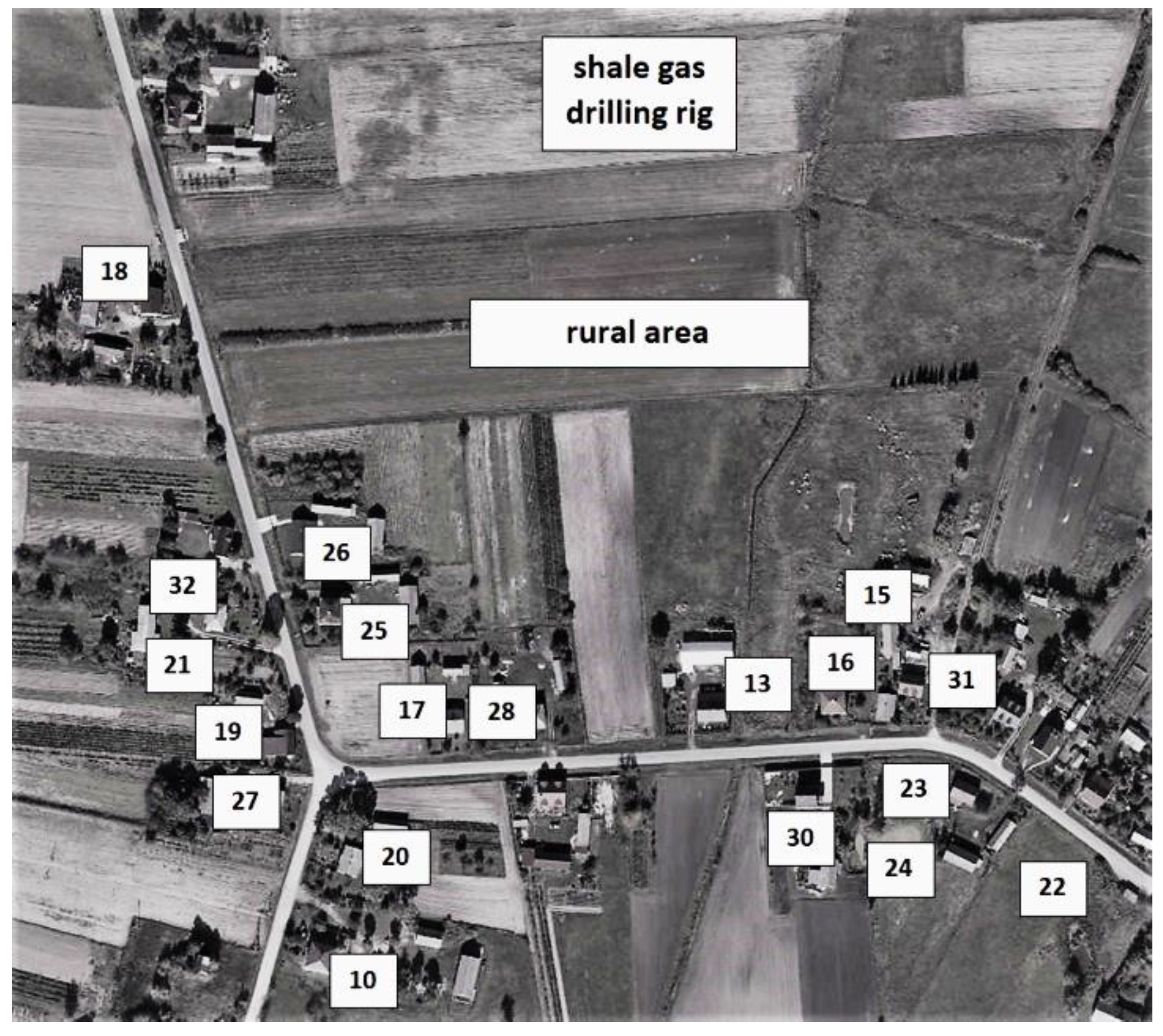
The analyzed water samples were taken from 17 dug wells located in the village of Syczyn and two deepwater wells, which constitute drinking water intakes for the Wierzbica commune in the Lubelskie Voivodeship in Poland (Figure 1). The sampling area is flattened and its height is in the range of 178–181 m above sea level. The study covered a rural area where agricultural activities are carried out. The dug wells are located in the immediate vicinity of the Natural Gas Processing Plant, where the shale gas well is located.
The closest of the wells is 220 m and the farthest is 600 m away from the plant site. The two deepwater wells are located 4.9 km and 6.75 km away on the opposite sides of the gas drilling rig. The groundwater samples were stored in a laboratory refrigerator at 4 °C until subjected to the standard analysis procedures in accordance with the American Public Health Association [21]. Table 1 specifies the methods and standards followed in the water quality parameters testing.
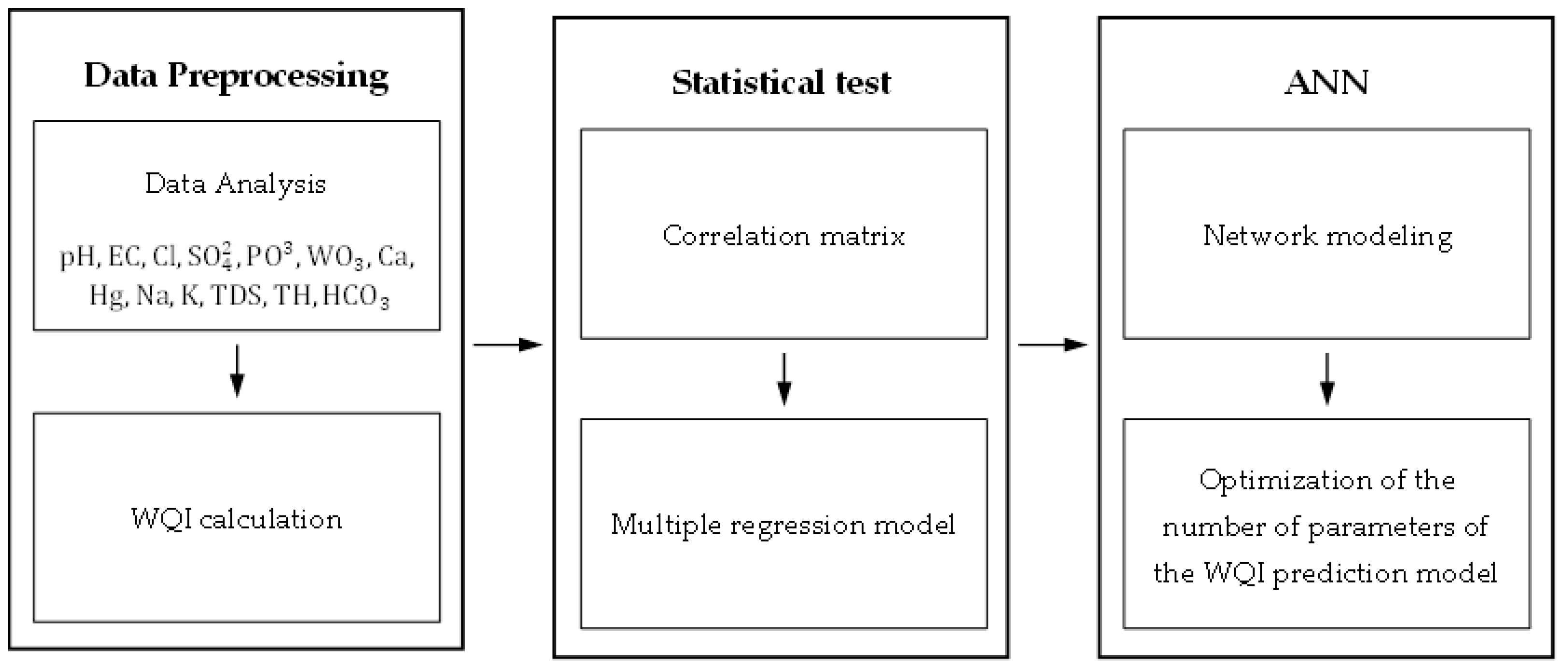
The methodology for the development of the WQI, MLR and ANN models is shown in the flowchart (Figure 2).
2.2. Water Quality Index
The Water Quality Index (WQI) is an assessment technique that reflects the complex impact of individual water quality parameters on the overall quality of water [22]. Typically, for the calculation of WQI, 10 important water quality parameters were selected, according to the drinking water quality standard recommended by the World Health Organization [23].
In this study, the physicochemical parameters in the three-step analysis of WQI were pH, EC, TDS, TH, Ca2+, Mg2+, Na+, K+, Cl−, HCO3−, SO42−, NO3− and PO43−.
In the first step, weights (wi) were assigned to each parameter on a 1–5 scale, reflecting their relative importance for drinking water quality. The weights for individual water parameters are presented in Table 2 [24].
In the second step, relative weights (Wi) were calculated from Equation (1):
where Wi is the relative weight, wi is the weight of each parameter, n is the number of parameters.
Thirdly, from the Formula (2) below, a quality rating scale (qi) was assigned to each parameter, by dividing its concentration in the water samples by its respective standard as per the WHO guidelines [23]
where qi is the quality rating, Ci is the concentration of each chemical parameter in each water sample in milligrams per liter; Si is the drinking water standard for each chemical parameter in milligrams per liter accordingly.
WQI was derived from Equations (3) and (4)
where is the subindex of i-th parameter, qi is the rating based on the concentration of i—the parameter, n is the number of parameters.
2.3. Selection of the ANN Input Parameters
Multiple regression was employed to establish the input parameters of the ANN model. The ANN was modeled in the R environment in the RStudio 1.0.153 program (Rstudio, Boston, MA, USA). The quality of the models was verified using the residual normality distribution with the application of the Shapiro–Wilk test. On the basis of the diagnostic plots of residues distribution against the predicted residues, the homoscedasticity of the residues and the absence of autocorrelation of residues were tested. Cook’s distance checked the existence of outliers in the regression model.
The multiple regression model allows examining the influence of a number of independent variables, i.e., water quality parameters (X1, X2, …, Xn) on the dependent variable WQI (Y). The Multiple Regression Model (5) is given below:
where:
—model parameters (regression coefficients) describing the influence of the j-th variable,
—random component (model residuals).
The measure of the model fitness is the multiple determination coefficient R2, the value of which is in the range <0;1>, calculated from the Formula (6):
where:
the value of water quality index for the i-th observation received from the model
the actual value of water quality index for the i-th observation
The coefficient involves comparing the variance of model residuals with the total variance of data. The closer it is to one, the better the fit to data. Conversely, the closer it is to zero, the worse the fit to data [26].
2.4. Modeling of the ANN
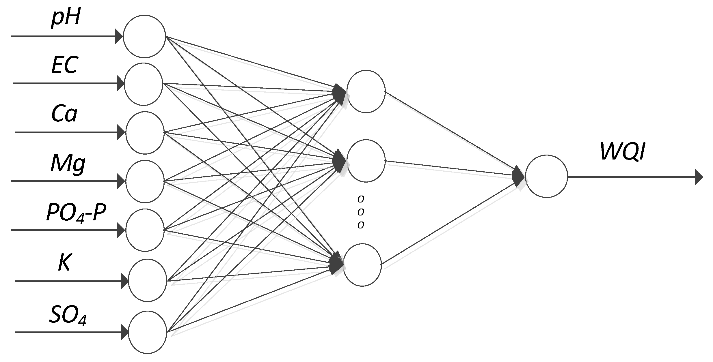
WQI prediction with the application of ANNs was performed using the Neural Network library in MatLab and Simulink computing environments (MathWorks, Massachusetts, USA). The number of input parameters was derived from the multiple regression analysis. The input parameters of the model were the physicochemical parameters EC, pH, Ca, Mg, PO4-P, K, SO42− (7 input neurons), and the output neuron—WQI. Subsequently, using the stepwise regression method, the models with ever fewer variables were tested. Modeling was performed using the Neural Network Fitting app, and the Levenberg–Marquardt algorithm for training. A two-layer feed-forward network with sigmoid hidden neurons and linear output neurons was used. The networks included one hidden layer. According to the literature, networks with a higher number of hidden layers are better fitting for higher complexity cases [27]. The number of neurons in the hidden layer (2 ÷ 10) was selected experimentally, as well as reflected the mean square error and the regression value R scores. The training set was 70%, and the test and validation sets were 15% each. A schematic representation of the ANN for the first model is shown in Figure 3.
Two measures of network quality were employed—mean square error (MSE) and regression R-value. MSE was calculated from the Equation below (7):
where n—number of cases in a given set; —the actual value of water quality index for the i-th observation; —a predicted value of water quality index for the i-th observation.
The regression coefficient R measures the correlation between outputs and inputs and is derived from (8):
where σy′—standard deviation of reference values, σy*—standard deviation of predicted values.
The higher the regression coefficient R and the lower the MSE, the better quality of the generated network is.
In order to compare the quality of WQI predictions for individual models, the root mean square error (RMSE) indicator will be used (9), calculated as:
where MSE—mean square error.
3. Results
3.1. Water Quality Index
The parameters of groundwater samples from the studied wells (Table 2) were juxtaposed with the drinking water quality guidelines defined by the WHO [23]. The contents of nitrate (V), chloride, magnesium, sodium, and bicarbonate (IV) ions did not exceed the limits in any of the tested wells. On the other hand, total hardness was several times higher than the value of TH specified in the WHO guidelines. Water pH was increased exclusively in well 15, and the concentration of sulfate (VI) in wells 18 and 19. The WHO standards were exceeded in the majority of wells for the following parameters: calcium concentration (except for wells 24 and 27—below 75 mg/L); potassium concentration (except for wells 16, 21–22, 28—below 10 mg/L); total dissolved solids (TDS) (except: 19, 21–26, 28, 30—below 500 mg/L) and for the phosphate (V) value (except wells 16, 18, 22–24, 30).
The calculated WQI is presented in Table 5. Wells 10, 15, 22, 24, 25, 28 are characterized by WQI < 50, which denotes water of excellent quality. The WQI value of the remaining wells was between 50.30 and 84.93, indicative of good water quality. None of the examined wells showed poor water quality.
In the first step, the correlation matrix between the variables was analyzed. Due to the singular form of the matrix with a set of variables, the variables were reduced.
3.2. WQI Modeling and Prediction
3.2.1. Multiple Regression Model
Given the high correlation coefficient between the variables of interest, i.e., EC (1.0) and TDS as well as TH and Ca (0.99), variables TDS and TH were removed. The remaining correlation coefficients between the independent variables were lower than 0.85 (the absolute value), which did not indicate an excessively strong correlation of the independent variables in the regression model.
After TDS and TH variables had been removed, it emerged that Cl−, SO42−, NO3−N, Na were insignificant in the regression model. Despite the high R2 of the model, 0.99, after verifying the assumptions, it was found that with a complete set of variables in the model, there is one outlier (Map 30) and no normal distribution of the residuals, for which reason, the model was rejected. The stepwise progressive regression produced a model that met the assumptions of the correct multiple regression: normal distribution of residuals, no residual autocorrelation, residual homoscedasticity, and no outliers. The coefficients in the model are shown in Table 6; the value of SO42− emerged as an insignificant variable, most likely owing to redundancy associated with high correlation with other variables. The determination coefficient R2 = 0.99 indicates a very good fit to the data model.
The model takes the following form:
Positive values of the model coefficients indicate a positive relationship between the dependent variables and the WQI score, while the negative ones denote the contrary. The results show that all the coefficients for the dependent variables are positive; hence, when the physicochemical parameters, EC, pH, Ca, Mg, PO43−, K, SO42− increase, the WQI value increases accordingly, thereby signifying an increase in water pollution.
3.2.2. ANN Modeling and WQI Prediction
In accordance with the results from the multiple regression model, the WQI variable was modeled by means of ANNs using EC, pH, Ca, Mg, PO43−, K, SO42− as input variables. From the executed ANN modeling, the best results were obtained for the network with five neurons, after 14 iterations. Other data, including performance validation and the rate of error decrease (gradient), are shown in Figure 4. The ANN performance was validated with MSE. The best validation result was exhibited by the network’s tenth iteration (Figure 5). In general, the error was found to decrease over successive training periods, but it is likely that it would start to increase in the validation dataset in the case when the network began to overfit the training data. The training was designed to stop after six consecutive increases in the validation error (or no decrease), and the best results were obtained from the iteration with the lowest validation error. Table 7 shows the network training results (MSE and Regression R-value) categorized into training, validation, and testing subsets.
The regression value (R) for training data is 0.9984, for validation data—0.9984 and the test data—0.9786, thus, in each case R > 0.95, which is typical of a good fit of the network. The overall regression coefficient was 0.9966, which confirms the high degree of overlap between the measurement points and the fit line with the ideal Y = T prediction line.
Subsequently, using the stepwise regression method, the models with ever fewer variables were tested. In the first step, the models with one variable removed were created. The best-performing model, i.e., the one with the minimal error, was the model with the rejected SO42− variable—Table 8. For comparison, the worst performance was delivered when Ca had been rejected (also Table 8). Having established that rejecting the SO42− variable improves the quality of the model, another variable was removed from the model in question and the models were compared. This time, the best model was the model with SO42− and PO43− variables rejected, where the mean square error is 0.651358, compared to the full model—1.25755. After the next variable was rejected, the mean square error started to increase, which proved that the quality of the model was deteriorating.
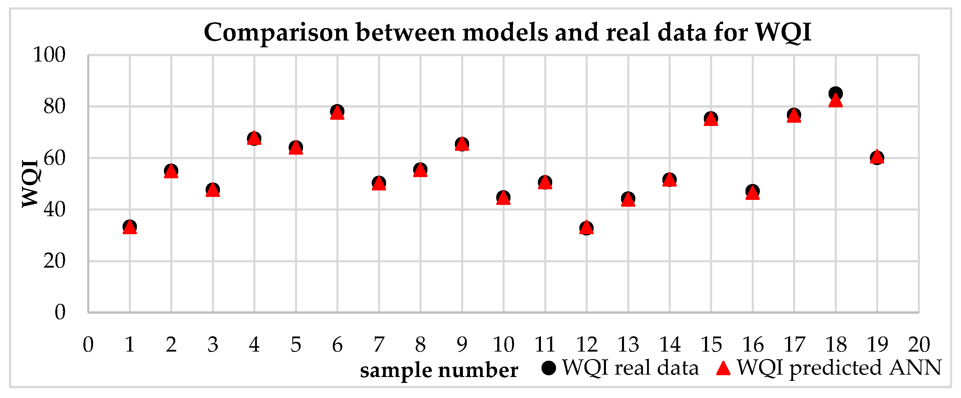
The optimization of the number of parameters and the quality of the network consisted in minimizing RMSE and the maximum error (%) relative to the WQI value. Table 8 shows two versions of the models. The models with one rejected variable were tested each time. The model with the best and worst parameters is presented. It can be seen that up to a point, the models have lower RMSE values when rejecting variables. The best network was obtained for the network with the following parameters: EC, pH, Ca, Mg, K, for which RMSE = 0.651258 and max% error (2.98%). The RMSE value obtained for this network was of a similar magnitude as in the case of the original multiple regression model (RMSE = 0.06167). Moreover, the good quality of this network is proven by R = 0.9992 and R2 = 0.9984. Next, after discarding the subsequent variables, the RMSE values began to increase and the properties of models deteriorated. Figure 6 presents a comparison of the experimental data and the data obtained from WQI prediction for the networks with optimal input parameters (EC, pH, Ca, Mg, K).
Despite the small discrepancies (RMSE = 0.06167), it can be concluded that the presented ANN models display an acceptable level of error and, therefore, emerge as reliable predictors supporting the decision-making processes [17].
4. Discussion
The drilling processes constitute a real threat involving the pollution of groundwater [28]. In accordance with legal regulations, the assessment of water quality in drilling areas must be controlled and constantly monitored. In the first part of this paper, the assessment of water quality indicators (Table 4) was performed according to the criteria defined by Sahu and Sikdar [25]. The results indicated that in 11 wells the water quality is good, and in 8, it is excellent (WQI < 50).
In the paper, an attempt was made to prove that ANN models are efficient tools for predicting the water quality, which can be employed for planning integrated water protection systems, while implementing good environmental management practices.
There are several advantages of employing the ANN method for predicting WQI over the computational approach. The latter method requires calculating the values of at least twelve water quality parameters (Table 1), which should be converted into partial indicators (Table 2). The formula for calculating the WQI is basically performed on sub-indices. Therefore, it is much easier to apply an existing ANN model that uses raw data without the need for additional recalculation. As few as five water quality parameters are required to build the model, which, among other things, reduces the cost of water quality monitoring.
The water quality prediction models are largely focused on rivers. The research object in this study involved the wells located in Poland, in the vicinity of a shale gas drilling rig. Thus far, no ANN models of water quality in drilling areas have been created in Poland. The presented modeling method can be adjusted for application in other drilling areas (coal, kerosene, gas). The authors believe that the application of artificial neural networks in various aspects of the environment constitutes a new approach to implementing good environmental management practices.
On the basis of results obtained via empirical studies on 19 wells located in the vicinity of a shale gas drilling rig, an ANN model of WQI was created for the water intakes located in shale gas drilling areas. Table 9 presents the results of the existing WQI models, including the one created by the authors.
The set of input variables in the model for WQI assessment can be composed in various ways. According to Nordin et al. (2021), the most common variable used for ANN modeling of the groundwater quality is SO42−, followed by Cl−, Mg, Ca, pH, TDS, and TH [19]. The analysis indicated that the above-mentioned parameters are strongly correlated with each other and were frequently selected as input parameters for the groundwater quality evaluation [40]. Input parameters accurately verify the groundwater quality, both for drinking and irrigation. The correlation analysis conducted in the paper indicated a strong correlation between the selected input data.
The presented model structure was optimized in order to minimize the number of input variables to the model while not compromising the quality of predictions. The input factors for building the neural network model were selected from the results of multiple regression. ANN validation with the use of linear regression analysis was proposed, e.g., by Flavelle (1992) [41]. Schenker and Agarwal (1996) proved that comparing regression models should be based on the closest adjustment of R-value [42]. The regression coefficient of the developed model reached R2 = 0.99, which indicates a very good fit to the data model. The multiple regression model showed that EC, pH, Ca, Mg, PO43−, K, SO42− are significant variables in the prognosis of WQI.
On the basis of the regression model, optimal input data for ANN model creation were selected. On the basis of network quality indicators, R, R2 and MSE, a network with five neurons in the hidden layer was selected as the best performer.
In order to develop a well-fitted and efficient ANN model (used for WQI prediction), it is necessary to appropriately select, i.e.,
- the number of neurons in the hidden layer
- dataset division: training, validation, test
- appropriate variables.
In the literature, there are various ways of dividing the dataset into training, testing, and validation data: Jian et al. (2020) created and optima WQI prediction model in the river using 70% training set as well as 15% test and 15% validation sets [34]; Nayayk et al. (2020), obtained an optimal WQI prediction model for the Godavari river using a training, validation, and testing set of 75%:15%:10%, respectively [32]. In turn, Al-Adhaileh and Alsaade created a WQI prediction model for selected rivers and lakes of India, using 70% for the training phase and 30% for the testing phase [30].
While creating the investigating model, the authors assumed the training, validation, and testing data ratio used by Jian et al. [34].
The number of neurons in the hidden layer constitutes another parameter used in developing a well-fitted model. The optimal number of neurons is determined using the trial-and-error method. It is expected that the number of hidden neurons should range from 11 to 11 [43]. In the presented studies, the model comprised five hidden neurons. Patki et al. (2021) developed an ANN model for WQI prediction in municipal distribution using the same number of neurons as in the model developed by the authors of this paper [30]. In turn, Yilma et al. (2018) obtained the most optimal model architecture using 15 hidden neurons that resulted in an R2 value of 0.93 [36].
The authors focused on selecting the least number of input data. The table shows that the number of input data for predicting the water quality differs, ranging from 6 [28] to 23 variables [39]. Moreover, the input data are rarely optimized for network creation, as in the case of the ANN model presented by Hore [14].
The models with a decreasing number of variables were tested using the backward stepwise regression method. First, the models with one variable removed were constructed to select the one with the minimum RMSE and the minimum percentage error in relation to the WQI value. In subsequent steps, other variables were removed until the WQI values began to increase in two subsequent iterations. From RMSE minimization and minimization of the maximum % error in relation to the WQI value, the optimal number of network parameters (EC, pH, Ca, Mg, K) was determined, under the constraint of maintaining the appropriate quality of this network (RMSE = 0.651258, max % error—2.98%). It was possible to create a model using only five types of input data, which showed an R = 0.9992, R2 = 0.9984; RMSE for the training set 0.0292, test set 0.2131, and validation set 1.3244. While analyzing the fit of the model to the actual data (comparing R and R2), the superior quality of the network was obtained in comparison to other presented models, even though fewer input parameters were used in the research (compared to other studies—Table 9).
The WQI predictions computed using the 5-5-1 network and trained by the Levenberg–Marquardt algorithm are strongly and positively correlated with WQI values of interest (r = 0.999, p < 0.05). This is further confirmed in Figure 6, delivering the comparison of the ANN-predicted WQI and the values of the models calculated on the basis of real data. On its basis, it can be concluded that the overall agreement between the real and simulated data is satisfactory. In turn, in the studies by Gazz et al. (2012), the relationship between the measured and simulated WQI of rivers (R = 0.977, p < 0.01; R2 = 95.4%; RMSE = 1.663) was obtained using the ANN model.
Koudari et al. (2021) created a WQIANN model for a region in south-east Algeria, characterized by the R2 value of 0.997 [43].
While comparing the created model with others (Table 9—values of R, R2, and RMSE), it can be stated that the general goodness of fit between the measured and simulated data is satisfactory.
Artificial neural network models should be used more frequently for predicting the quality of waters, as well as in other aspects of environmental protection.
The use of neural network models is possible even in the case of data deficiency, e.g., due to the unavailability, difficulty or high-cost expense of obtaining the actual figures. It also allows for the reconstruction of missing data, reducing costs and saving time for otherwise indispensable analyses, which can be a strong economic factor in science.
The obtained findings and drawn conclusions should encourage authorities and water quality management bodies to invest in the use of neural network modeling as a comprehensive and high-quality alternative to the standard WQI calculation methods.
5. Conclusions
The paper presented an alternative to an analytical method of water quality index determination, i.e., artificial neural network modeling for WQI prediction. The data used for conducting the study involved the results of empirical studies from 19 wells located in the vicinity of a shale gas drilling rig in Poland.
An ANN model was created based on the ANN approach with a two-layer feed-forward network with sigmoid hidden neurons and linear output neurons. The model was created using only five input parameters: EC, pH, Ca, Mg, and K. Optimal input data for ANN modeling were selected based on the results of multiple regression.
The ANN model was characterized by the correlation coefficient of 0.9992, as well as MSE equal to 0.0292, 0.2131, and 1.3244 for the training, testing and validating set, respectively. These results were obtained with the following set division: training (70%), validation (15%), and testing (15%), using the Neural Network Fitting app, and the Levenberg–Marquardt algorithm for training.
The advantage of using the ANN model proposed in this paper is the easy assessment of groundwater pollution levels; in addition, it enables the avoidance of lengthy calculations involved in prevalent conventional WQI.
In future works, the authors will attempt to effectively forecast water quality, using indicators that would depend on the proximity of pollution sources.
In future works, the authors are planning to employ other machine learning methods for groundwater quality assessment, including: deep neural network, Logistic Regression (LogR), Random Forest (RF). Decision Tree (DT) and K Nearest Neighbor (KNN). The results obtained using these methods will be compared and their impact on prediction quality will be investigated.
Moreover, forecasting of air pollution is within the scope of interest for the authors. The authors want to find out if the machine method learning can yield new information about air quality and the factors that have the greatest impact on this parameter.
Author Contributions
Conceptualization, J.K., M.K.; B.P. and W.C.; methodology, J.K., M.K.; B.P. and W.C.; software, M.K. and B.P.; validation, J.K., M.K.; B.P. and W.C.; formal analysis, J.K., M.K.; B.P. and W.C.; investigation, J.K. and W.C.; resources, J.K. and W.C.; data curation, J.K., M.K.; B.P. and W.C.; writing—original draft preparation, J.K., M.K.; B.P. and W.C.; writing—review and editing, J.K., M.K., B.P. and W.C.; visualization, J.K., M.K.; B.P. and W.C.; supervision, B.P.; project administration, M.K.; funding acquisition, J.K., M.K., B.P. and W.C. All authors have read and agreed to the published version of the manuscript.
Funding
This research received no external funding.
Data Availability Statement
Not applicable.
Conflicts of Interest
The authors declare no conflict of interest.
References
- Panaskar, D.B.; Wagh, V.M.; Muley, A.A.; Mukate, S.V.; Pawar, R.S.; Aamalawar, M.L. Evaluating groundwater suitability for the domestic, irrigation, and industrial purposes in Nanded Tehsil, Maharashtra, India, using GIS and statistics. Arab. J. Geosci. 2016, 9, 615. [Google Scholar] [CrossRef]
- Mukate, S.; Panaskar, D.; Wagh, V.; Muley, A.; Jangam, C.; Pawar, R. Impact of anthropogenic inputs on water quality in Chincholi industrial area of Solapur, Maharashtra, India. Groundw. Sustain. Dev. 2018, 7, 359–371. [Google Scholar] [CrossRef]
- Wagh, V.M.; Panaskar, D.B.; Mukate, S.V.; Gaikwad, S.K.; Muley, A.A.; Varde, A.M. Health risk assessment of heavy metal contamination in groundwater of Kadava River Basin. Model. Earth Syst. Environ. 2018, 4, 969–980. [Google Scholar] [CrossRef]
- Wagh, V.; Panaskar, D.; Muley, A.; Mukate, S.; Gaukwad, S. Neural network modelling for nitrate concentration in groundwater of Kadava River basin, Nashik, Maharashtra, India. Groundw. Sustain. Dev. 2018, 7, 436–445. [Google Scholar] [CrossRef]
- Bouslah, S.; Djemili, L.; Houichi, L. Water quality index assessment of Koudiat Medouar Reservoir, northeast Algeria using weighted arithmetic index method. J. Water Land Dev. 2017, 35, 221–228. [Google Scholar] [CrossRef]
- Kaurish, F.W.; Younos, T. Developing a standardized water quality index for evaluating surface water quality. J. Am. Water Resour. Assoc. 2007, 43, 533–545. [Google Scholar] [CrossRef]
- Babamiri, O.; Vanaei, A.; Guo, X.; Wu, P.; Richter, A.; Ng, K.T.W. Numerical Simulation of Water Quality and Self-Purification in a Mountainous River Using QUAL2KW. J. Environ. Inform. 2020, 37, 26–35. [Google Scholar] [CrossRef]
- Pesce, S.F.; Wunderlin, D.A. Use of water quality indices to verify the impact of Cordóba City (Argentina) on Suquía River. Water Res. 2000, 34, 2915–2926. [Google Scholar] [CrossRef]
- Scholten, H.; Kassahun, A.; Refsgaard, J.C.; Kargas, T.; Gavardinas, C.; Beulens, A.J.M. A Methodology to support multidisciplinary model-based water management. Environ. Model. Softw. 2007, 22, 743–759. [Google Scholar] [CrossRef]
- Salami, E.S.; Salari, M.; Ehteshami, M.; Bidokhti, N.T.; Ghadimi, H. Application of artificial neural networks and mathematical modeling for the prediction of water quality variables (case study: Southwest of Iran). Desalin. Water Treat. 2016, 57, 27073–27084. [Google Scholar] [CrossRef]
- Hatzikos, E.V.; Tsoumakas, G.; Tzanis, G.; Bassiliades, N.; Vlahavas, I. An empirical study on sea water quality prediction. Knowl.-Based Syst. 2008, 21, 471–478. [Google Scholar] [CrossRef] [Green Version]
- Yesilnacar, M.I.; Sahinkaya, E.; Naz, M.; Ozkaya, B. Neural network prediction of nitrate in groundwater of Harran Plain, Turkey. Environ. Geol. 2008, 56, 19–25. [Google Scholar] [CrossRef]
- Hore, A.; Dutta, S.; Datta, S.; Bhattacharjee, C. Application of an artificial neural network in wastewater quality monitoring: Prediction of water quality index. Int. J. Nucl. Desalin. 2008, 3, 160–174. [Google Scholar] [CrossRef]
- Dawood, A.S.; Hussain, H.K.; Hassan, A. Modeling of River Water Quality Parameters Using Artificial Neural Network—A Case Study. Int. J. Adv. Mech. Civ. Eng. 2016, 19, 51–55. [Google Scholar]
- Chen, Y.; Song, L.; Liu, Y.; Yang, L.; Li, D. A review of the artificial neural network models for water quality prediction. Appl. Sci. 2020, 10, 5776. [Google Scholar] [CrossRef]
- Bertolaccini, L.; Solli, P.; Pardolesi, A.; Pasini, A. An overview of the use of artificial neural networks in lung cancer research. J. Thorac. Dis. 2017, 9, 924–931. [Google Scholar] [CrossRef] [PubMed] [Green Version]
- Zali, M.A.; Retnam, A.; Juahir, H.; Zain, S.M.; Kasim, M.F.; Abdullah, B.; Saadudin, S.B. Sensitivity Analysis for Water Quality Index (WQI) Prediction for Kinta River, Malaysia. World Appl. Sci. J. 2011, 14, 60–65. [Google Scholar]
- Prasad, V.V.D.; Venkataramana, L.Y.; Kumar, P.S.; Prasannamedha, G.; Soumya, K.; Poornema, A.J. Water quality analysis in a lake using deep learning methodology: Prediction and validation. Int. J. Environ. Anal. Chem. 2020. [Google Scholar] [CrossRef]
- Palani, S.; Liong, S.Y.; Tkalich, P. An ANN application for water quality forecasting. Mar. Pollut. Bull. 2008, 56, 1586–1597. [Google Scholar] [CrossRef]
- Mischra, P.C.; Giri, A.K. rediction of Water Quality Indices by Using Artificial Neural Network Models: Prediction of Water Quality Indices. In Handbook of Research on Manufacturing Process Modeling and Optimization Strategies; IGI Global: Hershey, PA, USA, 2017. [Google Scholar] [CrossRef]
- American Public Health Association (APHA). Standard Methods for the Examination of Water and Wastewater, 21st ed.; American Public Health Association; American Water Works Association; Water Environment Federation: Washington, DC, USA, 2017. [Google Scholar]
- Ramakrishnalah, C.R.; Sadashivalah, C.; Ranganna, G. Assessment of water quality index for the groundwater in Tumkur Taluk, Karnataka state, India. Eur. J. Chem. 2009, 6, 523–530. [Google Scholar]
- WHO. Guidelines for Drinking Water Quality, 4th ed.; World Health Organization: Geneva, Switzerland, 2011. [Google Scholar]
- Varol, S.; Davraz, A. Evaluation of the groundwater quality with WQI (Water Quality Index) and multivariate analysis: A case study of the Tefenni plain (Burdur/Turkey). Environ. Earth Sci. 2015, 73, 1725–1744. [Google Scholar] [CrossRef]
- Sahu, P.; Sikdar, P.K. Hydrochemical Framework of the Aquifer in and around East Kolkata Wetlands, West Bengal, India. Environ. Geol. 2008, 55, 825–835. [Google Scholar] [CrossRef]
- Alexopoulos, E.C. Introduction to Multivariate Regression Analysis. Hippokratia 2005, 14, 23–28. [Google Scholar]
- Nguyen, T.T.; Nguyen, T.T.; Nguyen, N.A. Optimal Network Reconfiguration to Reduce Power Loss Using an Initial Searching Point for Continuous Genetic Algorithm. Complexity 2020, 2020, 2420171. [Google Scholar] [CrossRef]
- Patki, V.K.; Jahagirdar, S.; Patil, Y.M.; Karale, R.; Nadagouda, A. Prediction of water quality in municipal distribution system. Mater. Today Proc 2021, in press. [Google Scholar] [CrossRef]
- Al-Adhaileh, M.H.; Alsaade, F.W. Modelling and prediction of water quality by using artificial intelligence. Sustainability 2021, 13, 4259. [Google Scholar] [CrossRef]
- Vijay, S.; Kamaraj, K. Prediction of Water Quality Index in Drinking Water Distribution System Using Activation Functions Based Ann. Water Resour. Manag. 2021, 35, 535–553. [Google Scholar] [CrossRef]
- Nayak, J.G.; Patil, L.G.; Patki, V.K. Artificial neural network based water quality index (WQI) for river Godavari (India). Mater. Today Proc. 2021, in press. [Google Scholar] [CrossRef]
- Sakaa, B.; Brahmia, N.; Chaffai, H.; Hani, A. Assessment of water quality index in unmonitored river basin using multilayer perceptron neural networks and principal component analysis. Desalin. Water Treat. 2020, 200, 42–54. [Google Scholar] [CrossRef]
- Jian, B.T.P.; Mustafa, M.R.U.; Isa, M.H.; Yaqub, A.; Chia, H.Y. Study of the water quality index and polycyclic aromatic hydrocarbon for a river receiving treated landfill leachate. Water 2020, 12, 2877. [Google Scholar] [CrossRef]
- Vasanthi, S.; Kumar, A.S. Application of artificial neural network techniques for predicting the water quality index in the Parakai Lake, Tamil Nadu, India. Appl. Ecol. Environ. Res. 2019, 17, 1947–1958. [Google Scholar] [CrossRef]
- Yilma, M.; Kiflie, Z.; Windsperger, A.; Gessese, N. Application of artificial neural network in water quality index prediction: A case study in Little Akaki River, Addis Ababa, Ethiopia. Model. Earth Syst. Environ. 2018, 4, 175–187. [Google Scholar] [CrossRef]
- Hameed, M.; Sharqi, S.S.; Yaseen, Z.M.; Afan, H.A.; Hussain, A.; Elshafie, A. Application of artificial intelligence (AI) techniques in water quality index prediction: A case study in tropical region, Malaysia. Neural Comput. Appl. 2017, 28, 893–905. [Google Scholar] [CrossRef]
- Sakizadeh, M. Artificial intelligence for the prediction of water quality index in groundwater systems. Model. Earth Syst. Environ. 2016, 2, 8. [Google Scholar] [CrossRef]
- Gazzaz, N.M.; Yusoff, M.K.; Aris, A.Z.; Juahir, H.; Ramli, M.F. Artificial neural network modeling of the water quality index for Kinta River(Malaysia) using water quality variables as predictors. Mar. Pollut. Bull. 2012, 64, 2409–2420. [Google Scholar] [CrossRef] [PubMed]
- Che Nordin, N.F.; Mohd, N.S.; Koting, S.; Ismail, Z.; Sherif, M.; El-Shafie, A. Groundwater quality forecasting modelling using artificial intelligence: A review. Groundw. Sustain. Dev. 2021, 14, 100643. [Google Scholar] [CrossRef]
- Flavelle, P. A quantitative measure of model validation and its potential usefor regulatory purposes. Adv. Water Resour. 1992, 15, 5–13. [Google Scholar] [CrossRef]
- Schenker, B.; Agarwal, M. Cross-validated structure selection for neural networks. Comput. Chem. Eng. 1996, 20, 175–186. [Google Scholar] [CrossRef]
- Gupta, R.; Singh, A.N.; Singhal, A. Application of ANN for water quality index. Int. J. Mach. Learn. Comput. 2019, 9, 688–693. [Google Scholar] [CrossRef]
- Kouadri, S.; Kateb, S.; Zegait, R. Spatial and temporal model for WQI prediction based on back-propagation neural network, application on EL MERK region (Algerian southeast). J. Saudi Soc. Agric. Sci. 2021, 20, 324–336. [Google Scholar] [CrossRef]
Figure 1.
Research object (source: http://mapy.geoportal.gov.pl (accessed on 2 February 2021)).
Figure 1.
Research object (source: http://mapy.geoportal.gov.pl (accessed on 2 February 2021)).

Figure 2.
Flowchart of architecture of ANN and MLR models for WQI prediction.

Figure 3.
Schematic representation of an artificial neural network.

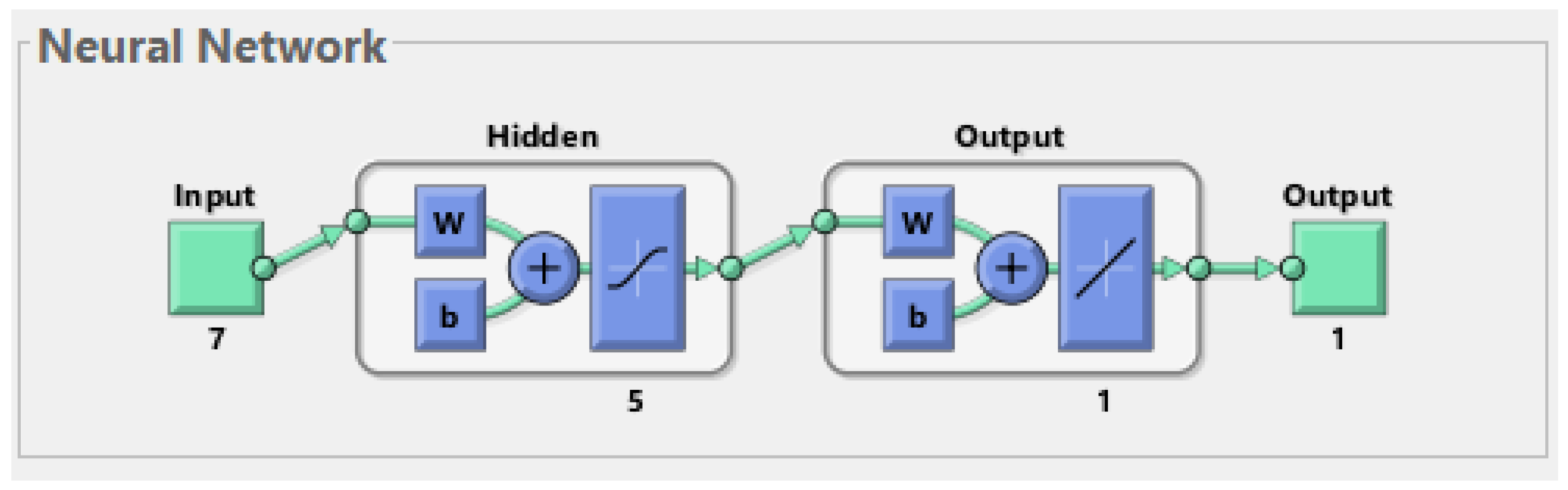
Figure 4.
Structure of the ANN.

Figure 5.
The best validation performance is 2.6218 at epoch 10.

Figure 6.
Comparison between models and real data for WQI.


Table 1.
Testing methods employed in the well water analysis.
| Parameter | Device | Norm |
|---|---|---|
| pH | ORION multimeter model: VERSA STAR (TermoFisher Scientific, London, United Kingdom; The Orion Navigator Pro computer software) | PN-EN 10390:1997 |
| Electrical conductivity (EC) | ORION multimeter model: VERSA STAR (TermoFisher Scientific, London, United Kingdom; The Orion Navigator Pro computer software) | PN-EN 27888:1999 |
| Total dissolved solids (TD) and total hardness (TH) | Titration kit | PN-C-04554-01:1971 |
| Na, K, Ca and Mg concentrations | ICP-OES JY 238 Ultrace (Jobin Yvon-Horriba, France, Analyst software) | PN-EN ISO 17294-2:2016-11 |
| Bicarbonate (IV) ions (HCO3−) | Titration kit | PN-C-04540-01:1990 |
| Nitrates (V) (NO3−) | Foss FIAstar 5000 flow analyzer with photometric detection (Foss, Hillerod, Denmark, software SoFIA) | ISO 13395 |
| Phosphates (V) (PO43−) | Foss FIAstar 5000 flow analyzer with photometric detection (Foss, Hillerod, Denmark, software SoFIA) | ISO/FDIS 15681-1 |
| Cl concentration | Titration kit | Mohr’s method |
| Sulfates concentration | HACH 8051 Spectrophotometer (Hach Company; AMES, USA, Application Software Drinking Water DOC022.98.90372) | Testing method PBL/CH/28/06 edition 02 of 07.11.2011 based on HACH 8051 |
Table 2.
The weights and relative weight of physicochemical parameters.
| Parameters | Weight (wi) | Relative Weight (Wi) |
|---|---|---|
| pH | 4 | 0.093 |
| EC | 4 | 0.093 |
| TDS | 5 | 0.116 |
| TH | 3 | 0.070 |
| Ca2+ | 3 | 0.070 |
| Mg2+ | 3 | 0.070 |
| Na+ | 2 | 0.047 |
| K+ | 2 | 0.047 |
| Cl− | 5 | 0.116 |
| HCO3− | 1 | 0.023 |
| SO42− | 5 | 0.116 |
| NO3− | 5 | 0.116 |
| PO43− | 1 | 0.023 |
Table 3.
Physicochemical parameter of water.
| Well No. | pH | EC | Cl− | SO42− | PO43− | NO3− | Ca2+ | Mg2+ | Na+ | K+ | TDS | TH | HCO32− |
|---|---|---|---|---|---|---|---|---|---|---|---|---|---|
| µS/cm | mg/L | ||||||||||||
| 10 | 7.55 | 375.05 | 17.75 | 84 | 6.52 | 9.13 | 65.16 | 2.65 | 13.45 | 15.8 | 240.00 | 166.19 | 300.01 |
| 13 | 7.08 | 762.56 | 28.40 | 79 | 6.33 | 10.24 | 107.57 | 9.49 | 31.01 | 75.27 | 487.68 | 295.35 | 251.52 |
| 15 | 8.07 | 578.73 | 28.40 | 85 | 2.81 | 0 | 101.62 | 6.18 | 16.79 | 45.52 | 369.92 | 267.58 | 243.13 |
| 16 | 7.06 | 775.46 | 35.50 | 64 | 0.44 | 2.73 | 195.11 | 3.42 | 20.92 | 4.60 | 496.00 | 479.07 | 30.05 |
| 17 | 6.95 | 1063.67 | 78.80 | 75 | 7.27 | 10.88 | 97.07 | 12.47 | 48.05 | 112.76 | 680.32 | 282.57 | 57.14 |
| 18 | 6.34 | 1153.35 | 106.50 | 240 | 0.47 | 11.65 | 161.02 | 17.42 | 70.72 | 46.89 | 737.92 | 455.31 | 111.21 |
| 19 | 6.80 | 712.58 | 46.15 | 53 | 0.58 | 12.14 | 94.45 | 9.74 | 43.55 | 27.45 | 455.68 | 265.11 | 164.17 |
| 20 | 6.97 | 875.94 | 31.95 | 63 | 6.91 | 8.63 | 84.79 | 10.92 | 46.97 | 100.69 | 560.00 | 246.93 | 267.35 |
| 21 | 7.25 | 762.24 | 10.65 | 81 | 0.28 | 12.26 | 170.84 | 10.03 | 21.92 | 14.70 | 487.68 | 448.37 | 221.33 |
| 22 | 7.12 | 487.51 | 28.40 | 14.4 | 0.10 | 11.18 | 108.15 | 7.39 | 5.82 | 3.99 | 311.68 | 288.11 | 287.46 |
| 23 | 6.99 | 529.26 | 3.55 | 5.4 | 0.14 | 7.78 | 128.15 | 12.05 | 7.72 | 5.48 | 338.56 | 354.92 | 134.52 |
| 24 | 6.95 | 356.78 | 0 | 29.3 | 0.16 | 6.67 | 72.84 | 2.95 | 9.59 | 8.61 | 227.84 | 185.72 | 93.31 |
| 25 | 7.42 | 581.92 | 14.20 | 38.1 | 1.08 | 10.31 | 88.02 | 4.99 | 23.75 | 39.8 | 371.84 | 230.28 | 84.57 |
| 26 | 6.89 | 779.26 | 21.30 | 63.6 | 0 | 12.50 | 88.24 | 8.37 | 25.38 | 95.09 | 498.56 | 244.68 | 154.28 |
| 27 | 6.73 | 1127.58 | 74.55 | 201 | 1.64 | 10.80 | 145.55 | 18.03 | 69.87 | 39.91 | 721.28 | 420.95 | 201.56 |
| 28 | 6.81 | 705.24 | 24.85 | 77.6 | 7.12 | 11.52 | 74.87 | 9.39 | 40.59 | 54.85 | 451.20 | 217.01 | 76.37 |
| 30 | 6.86 | 537.55 | 0 | 5.2 | 0.02 | 6.37 | 290.5 | 8.28 | 3.23 | 4.13 | 343.68 | 726.38 | 25.42 |
| 31 | 7.03 | 1290.18 | 53.25 | 201 | 1.93 | 11.94 | 169.31 | 16.51 | 44.85 | 132.40 | 825.60 | 471.33 | 47.68 |
| 32 | 7.11 | 949.68 | 35.5 | 57 | 1.09 | 11.06 | 100.45 | 10.46 | 59.45 | 88.11 | 607.36 | 282.37 | 46.79 |
| WHO limit | 6.5–8 | 500 | 250 | 250 | 0,5 | 45 | 75 | 50 | 200 | 10 | 500 | 100 | 500 |
Table 4.
The range and type of water for WQI [25].
Table 4.
The range and type of water for WQI [25].
| WQI Range | Water Types |
|---|---|
| <50 | Excellent water |
| 50–100 | Good water |
| 100.1–200 | Poor water |
| 200.1–300 | Very poor water |
| >300.1 | Water unsuitable for drinking purposes |
Table 5.
WQI values for samples of waters.
| Well No. | WQI | Well No. | WQI | Well No. | WQI |
|---|---|---|---|---|---|
| 10 | 33.22 | 20 | 55.38 | 26 | 51.48 |
| 13 | 54.98 | 21 | 65.34 | 27 | 75.30 |
| 15 | 47.62 | 22 | 44.69 | 28 | 47.04 |
| 16 | 67.49 | 23 | 50.50 | 30 | 76.66 |
| 17 | 64.07 | 24 | 32.75 | 31 | 84.93 |
| 18 | 78.10 | 25 | 44.13 | 32 | 59.98 |
| 19 | 50.30 |
Table 6.
Multiple regression model coefficients.
| b | Standard Error of b | p | |
|---|---|---|---|
| Constant | −0.313745 | 0.539090 | 0.572308 |
| EC | 0.033302 | 0.000239 | <0.000001 |
| Ca | 0.167108 | 0.000460 | <0.000001 |
| Mg | 0.301765 | 0.008489 | <0.000001 |
| pH | 1.171858 | 0.069464 | <0.000001 |
| PO43− | 0.053240 | 0.008371 | 0.000054 |
| K | 0.004032 | 0.001003 | 0.002023 |
| SO42− | 0.000869 | 0.000538 | 0.134578 |
Table 7.
Training ANN results.
| Data Subset | Mean Square Error (MSE) | Regression (R) Value |
|---|---|---|
| Training set (70%) | 0.56852 | 0.9984 |
| Validation set (15%) | 2.62182 | 0.9984 |
| Testing set (15%) | 4.93038 | 0.9786 |
Table 8.
Models with the best and worst parameters obtained in subsequent iterations.
| Step | ANN model | Rejected Variables | RMSE | Maximum Error Compared with WQI | R | R2 |
|---|---|---|---|---|---|---|
| 0 | Full model | 1.25755 | 6.02% | 0.9966 | 0.9932 | |
| I | Best | SO42− | 0.93944 | 6.44% | 0.9996 | 0.9992 |
| Worst | Ca | 7.370503 | 35.72% | 0.8818 | 0.7775 | |
| II | Best | SO42−, PO43− | 0.651358 | 2.98% | 0.9992 | 0.9984 |
| Worst | SO42−, Ca | 9.891332 | 39.17% | 0.7995 | 0.6392 | |
| III | Best | SO42−, PO43−, K | 0.856993 | 3.34% | 0.9990 | 0.9980 |
| Worst | SO42−, PO43−, Ca | 8.834689 | 41.91% | 0.7593 | 0.5765 | |
| IV | Best | SO42−, PO43−, K, pH | 0.90788 | 3.56% | 0.9990 | 0.9980 |
| Worst | SO42−, PO43−, K, Ca | 8.376916 | 38.13% | 0.7678 | 0.5895 |
Table 9.
Comparison of the proposed system with the existing models.
| Year | Test Object | Inputs (Variables) | Network Quality | Source |
|---|---|---|---|---|
| 2021 | Groundwater from wells located close to a shale gas extraction site | EC, pH, Ca, Mg, K | R = 0.9992 R2 = 0.9984 RMSE = 0.651258 | Proposed model |
| 2021 | Drinking water | pH, T-Alk, T-Hard, DO, TS, MPN | R = 0.999 MRE = 0.775 | Patki [29] |
| 2021 | Drinking water (India) | DO, pH, EC, BOD, N-NO3, Fecal Coliform, Total Coliform | R = 0.961 RMSE = 0.0029 | Al-Adhaileh [30] |
| 2021 | Drinking water distribution (India) | TDS, N-NO2+, N-NO3−, Ca, Mg, Na, K, Cl−, SO42−, CO32−, HCO3−, F−, pH, TH, SAR, RSC | Testing data RMSE = 0.057 R—no data Training data RMSE = 0.066 R—no data | Vijay [31] |
| 2021 | River (India) | pH, DO, BOD, Turbidity, TS | Training data MSE = 2.08 R = 0.997 Validation data MSE = 1.59 R = 0.997 Testing data MSE = 1.11 R—0.998 | Nayak [32] |
| 2020 | River (Algeria) | pH, WT, OS, TDS, NTU, N-NO3, P-PO4, BOD5, COD, Cl− | Testing data RMSE = 0.007 R2 = 0.811 Training data RMSE = 0.009 R2 = 0.929 | Sakaa [33] |
| 2020 | River (Malaysia) | TSS, BOD, COD, AN, DO, pH | Training data RMSE = 0.7001 R = 0.9964 Validation data RMSE = 2.174 R = 0.9829 Testing data RMSE = 1.186 R—0.9948 | Jian [34] |
| 2019 | Lake (India) | EC, TDS, Na, SSP, SAR, RSC, B | RMSE = 0.00617 R = 0.9907 | Vasanthi [35] |
| 2018 | River (Ethiopia) | TSS, NO3, NO2, T-N. T-Alk, TOC, COD, BOD, DO, T, EC, pH | RMSE = 1.97 R = 0,9993 | Yilma [36] |
| 2017 | River (Malaysia) | DO, BOD, COD, NH3-N, SS, pH | R2 = 0.9872 RMSE = 0.0157 | Hameed [37] |
| 2016 | Groundwater (Iran) | EC, TDS, NTU, pH, TH, Ca, Mg, SO42−, N-NO3, N-NO2, F−, P-PO4, Fe, Mn, Cu, Cr | Testing data RMSE = 7.71 R = 0.77 Training data RMSE = 0.01 R = 0.94 | Sakizadeh [38] |
| 2016 | Water river (Malaysia) | DO, BOD, COD, pH, SS, N-NH3 | R2 = 0.981 RMSE = 1.598 | Zali [17] |
| 2012 | River (Malaysia) | pH, EC, TDS, NTU, WT, BOD, DO, N-NH3, Mg, Cl, F, TH, Fe, Zn, As, Total caliform bacteria, E coli bacteria, SS, N-NO3, | RMSE = 1.633 R = 0.977 | Gazzaz [39] |
EC—electrical conductivity; pH—pondus hydrogenii; Ca—calcium, Mg—magnesium, K—potassium, TDS—total dissolved solids; N-NO2+, N-NO3—sum nitrite and nitrate; Cl−—chloride; SO42−—sulphate; CO32−—carbonate; HCO3−—bicarbonate; F−—fluorides; TH—total hardness; SAR—sodium absorption ratio; RSC—residual sodium carbonate; WT—water temperature; OS—oxygen saturation; NTU—turbidity; N-NO3,—nitrate; P-PO4—phosphate; BOD—biochemical oxygen demand; COD—chemical oxygen demand; B—boron; SSP—soluble sodium percent; DO—dissolved oxygen; N-NH3—ammonium; SS—sodium soluble percentage; Fe—iron; Mn—manganese; Cu—copper; Cr—chromium, Zn—zinc; As—arsenic.
Publisher’s Note: MDPI stays neutral with regard to jurisdictional claims in published maps and institutional affiliations. |
© 2021 by the authors. Licensee MDPI, Basel, Switzerland. This article is an open access article distributed under the terms and conditions of the Creative Commons Attribution (CC BY) license (https://creativecommons.org/licenses/by/4.0/).
Share and Cite
MDPI and ACS Style
Kulisz, M.; Kujawska, J.; Przysucha, B.; Cel, W. Forecasting Water Quality Index in Groundwater Using Artificial Neural Network. Energies 2021, 14, 5875. https://0-doi-org.brum.beds.ac.uk/10.3390/en14185875
AMA Style
Kulisz M, Kujawska J, Przysucha B, Cel W. Forecasting Water Quality Index in Groundwater Using Artificial Neural Network. Energies. 2021; 14(18):5875. https://0-doi-org.brum.beds.ac.uk/10.3390/en14185875
Chicago/Turabian StyleKulisz, Monika, Justyna Kujawska, Bartosz Przysucha, and Wojciech Cel. 2021. "Forecasting Water Quality Index in Groundwater Using Artificial Neural Network" Energies 14, no. 18: 5875. https://0-doi-org.brum.beds.ac.uk/10.3390/en14185875
Note that from the first issue of 2016, this journal uses article numbers instead of page numbers. See further details here.