Numerical Investigation for Three-Dimensional Multiscale Fracture Networks Based on a Coupled Hybrid Model

Abstract

The mismatching between the multi-scale feature of complex fracture networks (CFNs) in unconventional reservoirs and their current numerical approaches is a conspicuous problem to be solved. In this paper, the CFNs are divided into hydraulic macro-fractures, induced fractures, and natural micro-fractures according to their mode of origin. A hybrid model coupling various numerical approaches is proposed to match the three-dimensional multi-scale fracture networks. The macro-fractures with high-conductivity and wide-aperture are explicitly characterized by a mimetic Green element method-based hierarchical fracture model. The induced fractures and natural micro-fractures that have features of low-conductivity and small-openings are upscaled to the dual-medium grid and enhanced matrix grid through the equivalent continuum-medium method, respectively. Subsequently, some benchmark cases are implemented to confirm the high-precision and high-robustness of the proposed hybrid model that indeed accomplishes accurate modeling of fluid flow in multi-scale CFNs by comparing with commercial software tNavigator^®. Furthermore, an integrated workflow of simulation modeling for multiscale CFNs combined with a field example in Sichuan from China is used to analyzing the production information of fractured horizontal wells in shale gas reservoirs. Compared with the field production data from this typical well, it can be proved that the hybrid model has strong reliability and practicability.

1. Introduction

Shale has the characteristics of tight matrix with ultra-low permeability. At present, with the progress of hydraulic fracturing and horizontal well technology, shale gas production has been effectively improved [1,2]. Natural fractures developed in multiple tectonic stages, artificial hydraulic fractures reacted by improvement measures, and new connected induced fractures during hydraulic fracturing, combine to constitute a multiscale complex fractures system in the shale reservoir. The high-conductivity area formed by hydraulic fracturing is regarded as the stimulated reservoir volume (SRV), and the area without fracturing is the un-stimulated reservoir volume [3,4]. The SRV is composed of the multiscale complex fracture networks (CFNs) according to microseismic monitoring results [5,6,7], which leads to the flowing capability of fluids that are different from those in unstimulated formations. Consequently, the description and modeling of multiscale CFNs is the focus of current research. It is of great significance for petroleum engineers to investigate the fracture modeling of multistage fractured horizontal wells, which is one of the important approaches for accurate productivity evaluation and production planning.

At present, a large number of numerical methods are adopted to simulate the CFNs of multi-stage fractured horizontal wells with SRV, among which the first commonly used is the multicontinuum model [8,9,10]. One of the most practical models in the multicontinuum methods is the dual-medium model. The concept of dual-porosity was firstly presented by Barenblatt et al. [11] and superimposed the two media of matrix and fracture. Warren and Root [12] established the classical dual-porosity model and created a concept of inter-porosity flow to characterize the matrix–fracture mass transfer process. Then, Pruess et al. [13,14,15] developed a multiple interacting continua model that included a series of matrix control volumes nested in fracture control volumes, which can effectively describe the multiphase fluids and heat transfer in fractured reservoirs. Compared with explicit discretization, the multiple interacting continua approach can distinctly reduce the additional grids generated by subgridding. However, the above methods miss the matrix–matrix correlation and cannot make clear the fluid exchange between matrix cells. Subsequently, a developed model named the dual-porosity dual-permeability (DPDK) was presented by Blaskovich et al. [16] and Hill et al. [17] and it added the flux between matrix grids. However, there are still problems that lead to unaccepted results in the existence of highly-localized anisotropy and preferential channeling [18]. Overall, the multicontinuum model, such as the DPDK, is too idealistic to recover the geometrical feature of large-scale hydraulic fractures when it is applied to practical engineering problems.

Compared to the traditional multicontinuum model, the explicit discretization, such as the discrete fracture network (DFN) or model (DFM) [19,20,21] and the hierarchical fracture model (HFM) [22] that also known as the embedded discrete fracture model (EDFM) [23,24]. EDFM is a hot issue in the field of fractured reservoir simulation and has grown rapidly. DFM was firstly presented by Snow [25] and developed from single-phase flow to multiphase flow in fractured porous medium. The common numerical methods have been developed from finite element method [19,20] to control-volume finite element method [26,27,28], control-volume finite difference method [29], and mixed element method [30,31]. Among these, DFM can represent the real geometrical structure of different fractures with high resolution, but it is difficult to generate the unstructured grids and the simulation efficiency is poor when dealing with a large number of fractures. EDFM is a special dual-medium model considering the discrete distribution of fractures, which is usually regarded as an upgrade of DFM and dual-medium model. Li and Lee [23] developed the first generation of EDFM. They adopt a set of structured grids to discretize the computational domain, in which fractures are contained in these matrix grid-blocks such that fractures are segmented into many elements. This process saves the computational cost for superior matching grids and it can be easily introduced into the existing business simulators based on the finite difference method or finite volume method. Moinfar et al. [24] firstly proposed a practical embedded pre-processing algorithm for CFNs in a three-dimensional space and combined the DPDK model with EDFM to investigate the fluid flow behavior in fractured reservoirs. The research emphasis of 3D-EDFM is to work out the geometric relationship between matrix grid-blocks and fracture segments. However, the simulation accuracy cannot be guaranteed for low-connected and natural micro-fractures in EDFM because the grid conductivity of EDFM is calculated based on specific assumptions. When the permeability difference between the matrix and fracture is huge, errors can easily occur at the early stage.

In general, different models usually have their applicable conditions due to their limitations. There are many types of fractures according to different geological characterization and formation processes. These fractures are in the multi-scale coexisting state and fractures in different scales have different influences and contributions to reservoir fluid flow. Many studies had adopted a single method to deal with multi-scale fractures in actual reservoirs, which is unreasonable and insufficient. Consequently, the purpose of this paper is to classify scales of fractures during modeling and select the optimal simulation method respectively. Aiming at the contradiction between the simulation accuracy and the simulation efficiency of existing numerical simulation methods, authors adopted the different simulation methods for different scale fractures respectively and proposed a hybrid model coupling various numerical methods for capturing the behavior of fluids in multiscale CFNs.

The present work develops a hybrid model for modeling the complex fracture networks in fractured shale reservoirs in which the multi-scale fractures are classified into the hydraulic macro-fractures, induced meso-fractures, and natural micro-fractures. The characterization of three-dimensional ellipsoidal macro-fractures is the focus of our research. For this purpose, the discrete flux operator derived from mimetic FDM is firstly adopted to approximate the boundary integral of the product of fundamental solution and edge-normal flux in GEM, which improves the accuracy of matrix-fracture mass transfer. Then, a coupling method for multiscale fractures is introduced (in Section 2). The hybrid model is benchmarked against the tNavigator^® in Section 3. A field case of shale gas reservoirs from the Sichuan Basin of southwestern China is practiced by our model (in Section 4). Finally, some conclusions on the presented multi-scale fractures model are given.

2. Methods

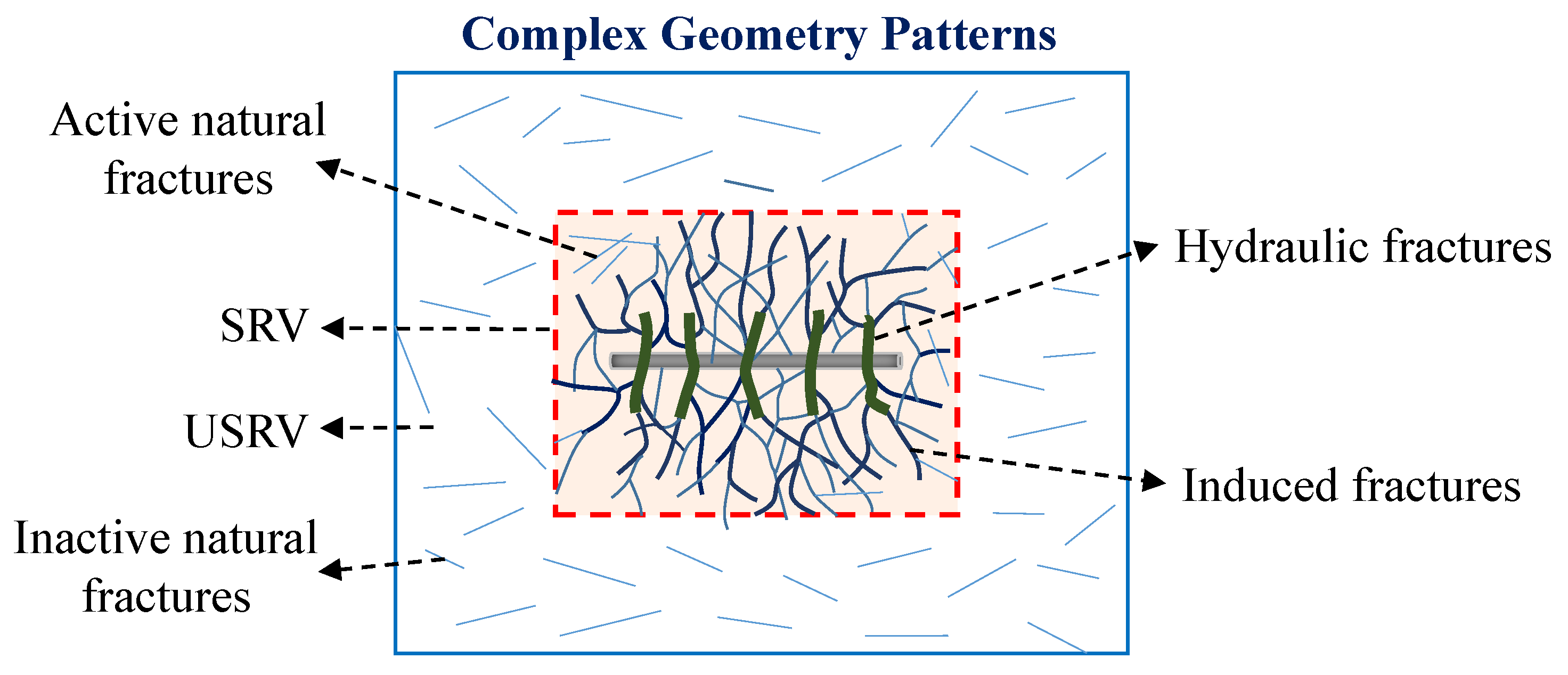
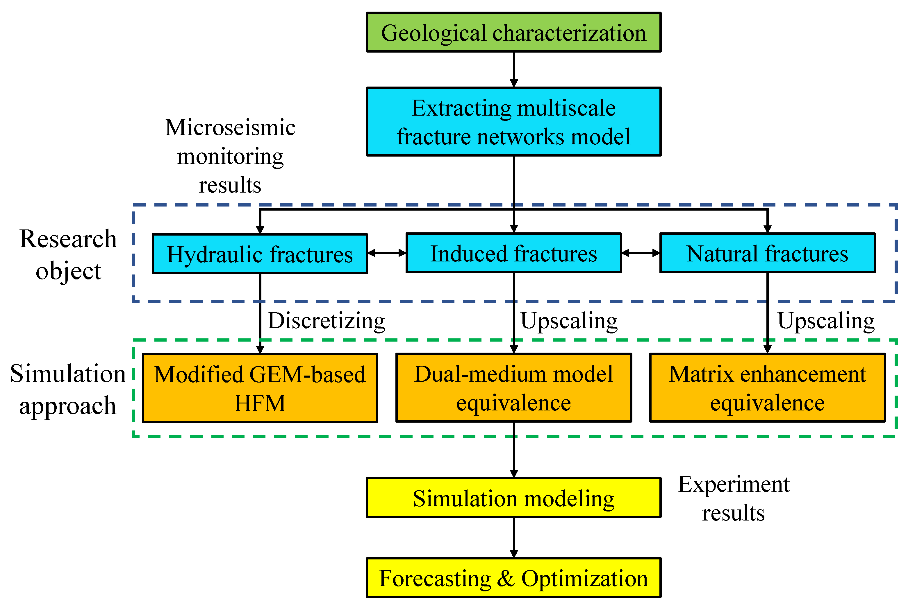
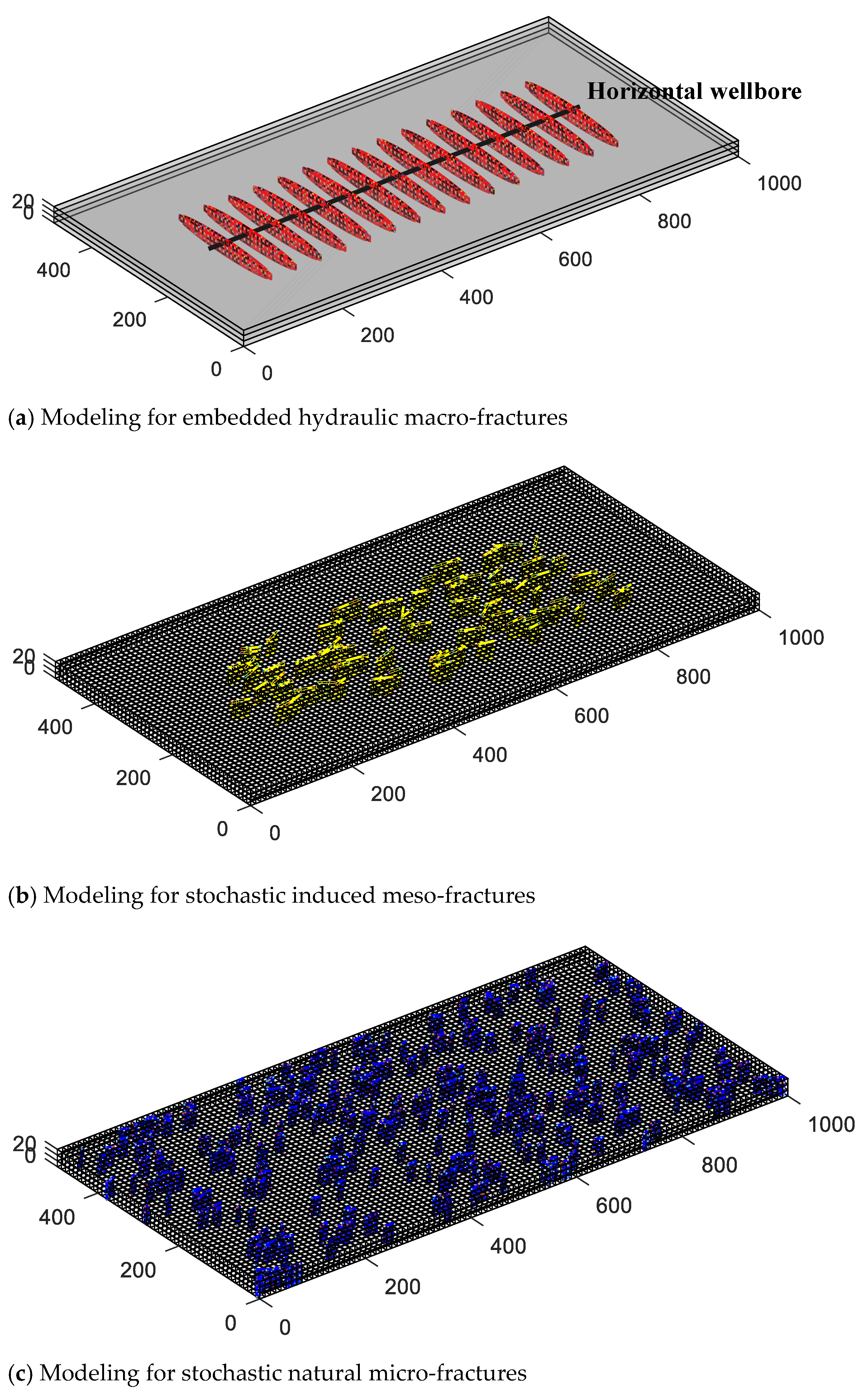
2.1. Classification for Multi-Scale Fractures

The shale gas reservoir has the geological characteristics of natural fracture development. However, these natural fractures are mostly closed due to the effect of in-situ stress, which does not improve the permeability of the whole gas reservoir in the initial state. Hydraulic fracturing, which is realized by injecting the fracturing fluids and the proppant materials with high pressure to open the formation, has been successfully employed for enhancing shale gas recovery for many years. Some natural fractures are activated and connected in the SRV area during hydraulic fracturing due to the change of the stress field and the filtration of a lot of fracturing fluids, which together with the hydraulic fractures to react the complex fracture networks. The distribution of hydraulic fractures, induced fractures, open and unopened natural fractures in shale gas reservoirs after SRV fracturing are shown in Figure 1. The SRV has greatly improved the overall reservoir permeability and made a great contribution to total well production. It should be noted that the SRV region is not necessarily a regular rectangle and it can be of arbitrary shape according to the distribution of multiscale fractures for actual reservoirs.

Generally, fractures can be classified into three scale levels: macro-scale, meso-scale, and micro-scale according to the aperture (flow conductivity) or length [32]. Hydraulic fractures can be regarded as macro-fractures because the permeability of hydraulic fractures is much larger than that of matrix domains, and it has a decisive effect on fluid flow. Generally, macro-fractures can be handled by EDFM because the morphology and flow behaviors of hydraulic fractures can be fully and explicitly characterized [33,34,35]. Induced fractures can be regarded as meso-scale fractures. When the number of fractures is small and the connectivity is poor, EDFM can also be used for fine simulation of induced fractures. However, when there is a large number of induced fractures that be connected to form fracture networks, the pretreatment process is unnecessarily complex and resulting in high computational cost [36]. In this condition, the efficient and stable dual-medium model can be used for equivalent simulation, and high simulation efficiency can be maintained with only a small part of accuracy loss [37]. The porosity and permeability of natural fractures are usually small and can be regarded as micro-fractures. Therefore, natural fracture properties can be directly equivalent to the matrix by the single-medium equivalent model, which effectively improves the computing efficiency.

With the application of high-resolution technologies such as microseismic and imaging logging, macro-scale hydraulic fractures have high recognition and precision. The dominant pretreatment mode of EDFM can make macro-fracture maintain high confidence to a large extent [38]. The meso-scale induced fractures and micro-scale natural fractures are mainly limited by existing detection techniques and are generally predicted by stochastical simulation methods because their confidence is usually low. For continuous medium models such as the dual-medium model and the single-medium equivalent model, it is easy to adjust the properties of low-confidence random fractures in the history matching stage, such as adjusting the shape factor, matrix equivalent permeability, etc.

At present, scales of fractures are mainly classified according to their geometry size [22,32]. However, the geometry size of fractures is relative, and the classification criteria also have big differences for different regions when solving practical problems. Therefore, the author believes that there are no fixed fracture-scale classification criteria. The classification of macro-scale, meso-scale, and micro-scale in the paper only refer to three types of fractures, respectively corresponding to three approaches with advantages and disadvantages in simulation accuracy and computational efficiency. Sometimes all-scale fractures can be discretized and it is completely unnecessary to classify all the fractures when it comes to the situation of a small number of fractures, high confidence, or advanced computer configuration resources. Conversely, it can flexibly select the equivalent method of dual-medium or single-medium to implicitly characterize the meso-scale and micro-scale fractures when there are a large number of fractures in reservoirs, the fracture confidence is low, or computer resources are poor. Accordingly, it is necessary to choose between the simulation accuracy and the computational efficiency according to the specific situation. To summarize, the classification of multiscale fractures depends on fracture geometric sizes, fracture confidence, practical computer resources, and other objective factors, and it should be comprehensively considered in practical applications.

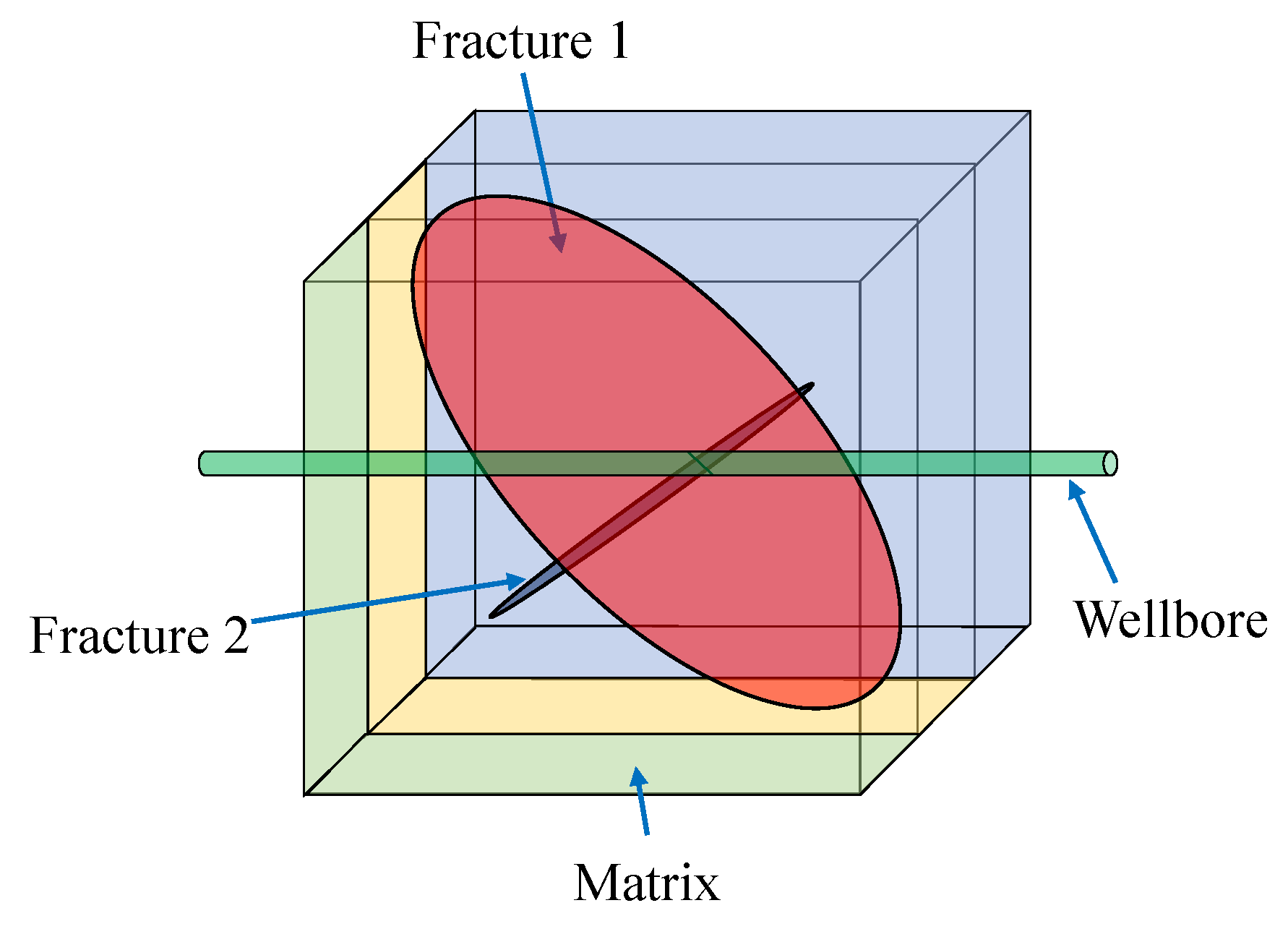
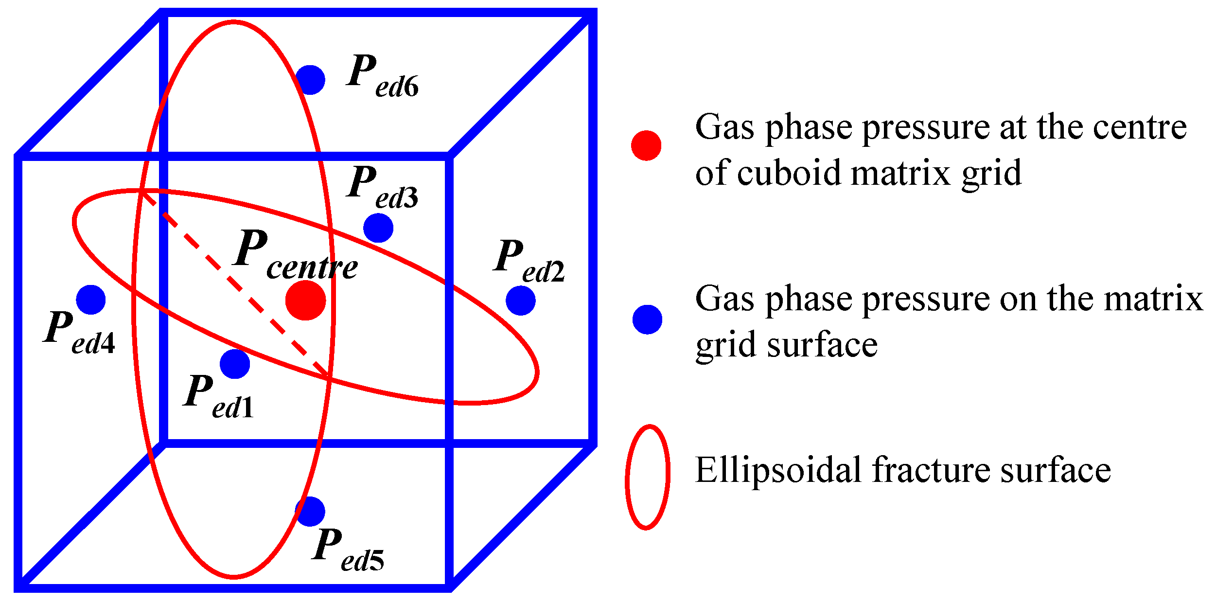
2.2. Parameterization of 3D Ellipsoidal Macro-Fracture

The existence of ellipsoidal fractures is especially common in three-dimensional and can provide a more comprehensive analysis than classical planar fractures. Because the classical homogeneous planar fracture model is the simplified shape according to the ellipsoidal fracture model [39]. However, there are few studies about the characterization method for ellipsoidal-shaped fractures in the three-dimensional reservoir. Macro-fractures need to be dimensionally reduced in the pre-processing algorithm of 3D-EDFM, which means a two-dimensional plane or curved surface is used to describe a hydraulic fracture in 3D reservoirs. Generally, the fracture is a two-dimensional curved surface when three-dimensional Euclidean space is used to describe the three-dimensional reservoir. The two-dimensional fracture plane can be uniquely defined by the first and second basic forms of the curved surface and a given base vector according to the classical curved surface theory in differential geometry. However, it is difficult to obtain the connection relationship between the fracture surface and matrix grids, and solve the geometric parameters of corresponding fracture grids if the fracture surface is represented by the 2D curved surface. Therefore, the fracture is generally simplified as a 2D plane in 3D-EDFM [36]. This paper uses 2D-plane to describe the high-conductive macro-fracture in 3D reservoirs, that is, a fracture corresponds to a 2D-plane.

To determine a 2D plane in a 3D-Euclidean space, it is necessary to first determine the direction of A₀ at a certain point on the plane, that is, the reference vector α₀ and two linearly independent (i.e., orthogonal) vectors α₁ and α₂ on the fracture plane. These two linearly independent vectors constitute two basis vectors of the local coordinate system with A₀ as the origin of the plane. The points on the fracture plane can be expressed as:

$$r={\alpha }_0+u{\alpha }_1+v{\alpha }_2$$

(1)

where r represents the vector diameter of the point on the fracture plane; α₀ is the reference vector; α₁ and α₂ are two linearly independent vectors selected on the fracture plane; u and v are corresponding parameters, i.e., even pair (u,v) (i.e., coordinates in the local coordinate system {A₀;α₁,α₂}) and points on the fracture plane.

Generally speaking, there are two types of fractures: rectangular fracture and ellipsoidal fracture. In this paper, the ellipsoidal shape is useThe regular italics of the formula and the text are not uniform, please confirmd to characterize the fractures in three-dimensional space because the ellipsoidal fractures are especially common in the real scenario and much more fit the engineering reality. The realization of ellipsoidal fracture is the combination of Equations (1) and (2), that is, Equation (3), in which the properties u and v need to satisfy the relationship f(u,v) ≤ 0, where f (u,v) = 0 to determine the boundary of fracture, and f (u,v) < 0 to determine the interior of fracture. The diagram of ellipsoidal fracture is shown in Figure 2.

$$\frac{u^2}{a^2}+\frac{v^2}{b^2}-1\le 0$$

(2)

$$f\left(u,v\right)=\frac{u^2}{a^2}+\frac{v^2}{b^2}-1$$

(3)

where a represents the length of the semi-major axis, and b represents the length of the semi-minor axis. Note that a and b are from the center outwards. We can determine the size of an elliptic plane by the values of a and b.

2.3. Mathematical Models for Matrix

2.3.1. Control Equations of Gas-Water Two-Phase Flow

Shale gas reservoir is generally divided into two parts: matrix and fracture, then mathematical models of flow in matrix and fracture are established respectively. This paper studies the three-dimensional flow problem and the assumptions are as follows:

(1)

Shale reservoir is homogeneous and equal thickness;

(2)

Compressible reservoir fluid is isothermal flow, and obeys Darcy’s law;

(3)

Mixed gas can be considered to be simplified as a single component CH₄;

(4)

Two-phase flow (gas & water) and the effect of dissolved gas in the water are considered;

(5)

The gravity term is considered on the fluids flow.

Then, the gas control equation in shale bedrock can be written as [36]:

$$\begin{array}{l}\nabla \cdot \left\{\frac{k{k}_{rg}}{B_g{\mu }_g}\left[\nabla p_g-{\rho }_{gsi}g\nabla \left(\frac{D}{B_{\mathrm{g}}}\right)\right]+\frac{R_{s}k{k}_{rw}}{B_w{\mu }_w}\left[\nabla p_w-{\rho }_{wsi}g\nabla \left(\frac{D}{B_w}\right)\right]\right\}\\ +q_{gsi}\delta +R_s{q}_{wsi}\delta +q_{diff}=\frac{\partial }{\partial t}\left(\frac{\varphi s_g}{B_g}+\frac{\varphi R_s{s}_w}{B_w}\right)\end{array}$$

(4)

where k indicates permeability attribute and the relative permeability is denoted with the subscript g for the gas phase and $w$ for the water phase respectively, likewise, B_g and B_w represent gas and water volume factor respectively; μ represents corresponding fluid viscosity; p represents corresponding fluid pressure; s represents corresponding fluid saturation; ρ_gsi and ρ_wsi indicate gas and water density under standard ground conditions respectively; q_gsi and q_wsi represent gas and water production rate under standard ground conditions respectively. In addition, symbol g represents gravitational acceleration; D indicates reservoir depth; R_s represents gas solubility; ϕ represents porous media porosity; δ is the Dirac function; q_diff is the flux rate of gas diffusion into the matrix grid.

The water control equation for matrix can be expressed as:

$$\nabla \cdot \left[\frac{k{k}_{rw}}{B_w{\mu }_w}\left(\nabla p_w-{\rho }_{wsi}g\nabla \left(\frac{D}{B_w}\right)\right)\right]+q_{wsi}\delta =\frac{\partial }{\partial t}\left(\frac{\varphi s_w}{B_w}\right)$$

(5)

Equations (4) and (5) are usually solved discretely by FDM or FVM. The matrix–fracture fluid exchange can be regarded as the interflow between two adjacent control volumes. In this paper, a coupling method is used for modeling the transient matrix–fracture fluid exchange according to the multi-scale feature of CFNs. We begin with a detailed introduction of the multiscale coupling method in Section 2.4 and Section 2.5.

2.3.2. Gas Desorption and Diffusion

The gas desorption effect is one of the most striking characteristics of shale rock, which is significantly distinguished from conventional gas reservoirs. At present, the frequently used method to describe the gas desorption phenomenon is the Langmuir equation [40]. It assumes that the gas adsorption is a single molecular layer, which was initially adopted in coalbed methane. For single-component gas, the Langmuir isothermal adsorption-desorption theory can be written as follows:

$$\overline{C}=V_L\frac{p_g}{P_L+p_g}$$

(6)

where $\overline{C}$ is adsorption concentration at equilibrium; V_L indicates the Langmuir volume; P_L represents the Langmuir pressure. The V_L represents the maximum gas adsorption amount obtained by the experiment test, and P_L is the pressure when the adsorption amount reaches half of the maximum adsorption amount. The Langmuir pressure in the Langmuir isothermal coefficient model can be obtained by fitting the experimental data.

In general, the process of gas desorption from the matrix into the macropore is assumed to be an instantaneous adsorption process, which means the gas concentration in fractures reaches equilibrium adsorption concentration instantaneously when the pressure changes. However, it takes a certain time for the desorption gas to diffuse from micropores into macropores due to the extremely-low matrix permeability. The gas diffusion flux of per-unit volume in matrix according to Fick’s law can be expressed as follows [41]:

$$q_{diff}={\rho }_{m}v\left(C_c-C_c^{\infty }\right)$$

(7)

where ρ_m is the matrix density; C_c is the current adsorption concentration of matrix; $C_c^{\infty }$ is the current equilibrium adsorption concentration, and it can be obtained from the Langmuir isotherm model (Equation (6)). The diffusion velocity v is used to characterize the diffusion speed of desorption gas into macropores, which can be obtained by fitting the time curve of adsorption volume.

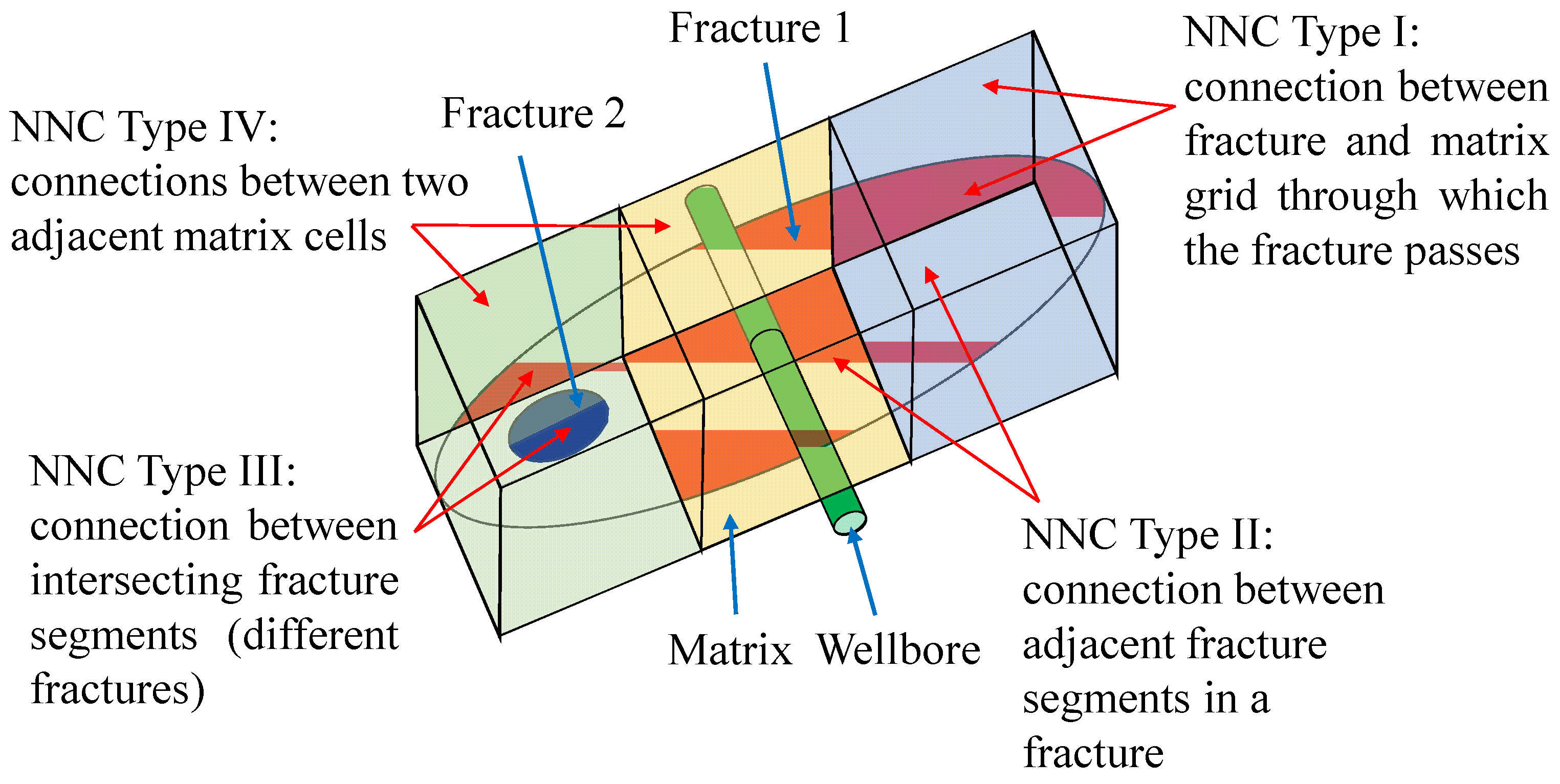
2.4. Coupling Method for Multiscale Fractures

2.4.1. Mass Transfer in Hydraulic Macro-Fractures

The conductivity calculation is an important step in the solution of fluid exchange capacity between adjacent grids when the EDFM is used to simulate macro-fractures. The expression contains three types of grid conductivity: matrix–matrix, matrix–fracture, and fracture–fracture. To determine the specific discrete format of control equations between fracture elements, the focus is to obtain the conductivity between fracture elements. The approximation of geometric factor in conductivity is associated with the connection relationship between matrix cell and fracture element. There are four types of non-neighboring connection (NNC) when dividing the fracture segments by matrix cell boundary (Moinfar et al. [24]; Rao et al. [36]; Du et al. [42]), which is illustrated in Figure 3. The significance of introducing NNC is to realize the mass transfer between adjacent grids in both theoretical and computational models. The transmissibility coefficient in NNC is calculated as follows [24]:

$$T_{\mathrm{NNC}}=\frac{K_{\mathrm{NNC}}{A}_{\mathrm{NNC}}}{{〈d〉}_{\mathrm{NNC}}}$$

(8)

where K_NNC represents the effective permeability of the NNC; A_NNC indicates the contact area of the NNC; ${〈d〉}_{\mathrm{NNC}}$ indicates the feature distances related to NNC.

As noted above, the matrix–fracture fluid exchange process is characterized by the geometric index in the conductivity term. In previous EDFMs, many researchers adopt the Equation (9) to approximate the average normal distance ${〈d〉}_{\mathrm{NNC}}$ which assumed that the pressure changes linearly in the normal direction to each fracture in a matrix gridblock (Li and Lee [23]; Moinfar et al. [24]; Hajibeygi et al. [43]). However, this assumption applies only to steady-state flow. Due to the huge difference between ultra-low matrix permeability and ultra-high fracture permeability, this linear steady assumption will lead to low calculation accuracy.

$${〈d〉}_{\mathrm{NNC}}=\frac{{\displaystyle {\mathrm{\int }}_V{x}_{n}dv}}{V_m}$$

(9)

where $dv$ represents the matrix volume cell; $x_n$ represents the normal distance of matrix cell from the fracture; V_m represents the volume of a matrix cell.

In this study, we adopt a modified Green element method (GEM) to calculate the transmissibility term in EDFM and aims to accurately characterize the transient matrix–fracture mass transfer term. The assumptions are the list:

(1)

Matrix–fracture mass transfer is the unsteady flow;

(2)

Matrix grid only flows to the fractures within the grid, and there is no fluid exchange with fractures in the adjacent grids;

(3)

The upstream weight is used to calculate the fluid mobility in the multiphase fluid exchange between matrix and fracture.

The unsteady mass conservation equation of gas components in anisotropic media in matrix grid including fracture grid is shown in Equation (10). The gas desorption does not need to be considered in fractures, which is different from the mass conservation equation in matrix. To simplify the equation form, the gas dissolution term is not considered in Equation (10).

$$\frac{\partial }{\partial x}\left(\frac{k_x{k}_{rg}}{\mu B_g}\frac{\partial p}{\partial x}\right)+\frac{\partial }{\partial y}\left(\frac{k_y{k}_{rg}}{\mu B_g}\frac{\partial p}{\partial y}\right)+\frac{\partial }{\partial z}\left(\frac{k_z{k}_{rg}}{\mu B_g}\frac{\partial p}{\partial z}\right)-{\tilde{q}}_{gmf}=\frac{\partial }{\partial t}\left(\frac{\varphi s_g}{B_g}\right)$$

(10)

In this matrix grid, the permeability is a constant, so the above formula can be transformed into an unsteady flow equation in equivalent isotropic medium through simple linear coordinate transformation, so that:

$$X=\sqrt{\frac{K_a}{k_x}}x,\hspace{1em}Y=\sqrt{\frac{K_a}{k_y}}y,\hspace{1em}Z=\sqrt{\frac{K_a}{k_z}}z$$

(11)

where $K_a=\sqrt[3]{k_x{k}_y{k}_z}$ represents the permeability of an equivalent isotropic medium.

Based on the above linear variable substitution, Equation (10) can be rewritten as:

$$\frac{{\partial }^{2}p}{\partial X^2}+\frac{{\partial }^{2}p}{\partial Y^2}+\frac{{\partial }^{2}p}{\partial Z^2}-\frac{\mu B_g}{K_a{k}_{rg}}{q}_{gmf}=\frac{\mu B_g}{K_a{k}_{rg}}\frac{\partial }{\partial t}\left(\frac{\varphi s_g}{B_g}\right)$$

(12)

By integrating the two ends of the above formula with time and adopting the implicit format, we can get:

$${\left(\frac{{\partial }^{2}p}{\partial X^2}+\frac{{\partial }^{2}p}{\partial Y^2}+\frac{{\partial }^{2}p}{\partial Z^2}-\frac{\mu B_g}{K_a{k}_{rg}}{q}_{gmf}\right)}^{t+\mathrm{\Delta }t}=\frac{1}{\mathrm{\Delta }t}{\left(\frac{\mu B_g}{K_a{k}_{rg}}\right)}^{t+\mathrm{\Delta }t}\left[{\left(\frac{\varphi s_g}{B_g}\right)}^{t+\mathrm{\Delta }t}-{\left(\frac{\varphi s_g}{B_g}\right)}^t\right]$$

(13)

Inspired by the idea of mimetic FDM [44], we utilize the discrete flux operator derived from mimetic FDM to approximate the boundary integral of the product of fundamental solution [45] and edge-normal flux in GEM. We present several main steps in the model derivation.

The corresponding boundary integral equation of Equation (13) is obtained as follows:

$$\begin{array}{l}c(\alpha ,\beta ,\gamma )p(\alpha ,\beta ,\gamma ,t+\mathrm{\Delta }t)={\displaystyle {\int }_{\partial \mathrm{\Omega }}p}(x,y,z,t+\mathrm{\Delta }t)\frac{\partial G_M(x,y,z;\alpha ,\beta ,\gamma )}{\partial n}\cdot ds(x,y,z)\\ -{\displaystyle {\mathrm{\int }}_{\partial \mathrm{\Omega }}{G}_M}(x,y,z;\alpha ,\beta ,\gamma )\frac{\partial p(x,y,z,t+\mathrm{\Delta }t)}{\partial n}\cdot ds(x,y,z)\\ +{\left(\frac{{\mu }_g{B}_g}{K_a{k}_{rg}}\right)}^{t+\mathrm{\Delta }t}{\displaystyle {\mathrm{\int }}_{\mathrm{\Omega }}{G}_M}(x,y,z;\alpha ,\beta ,\gamma )q_{gmf}(x,y,z,t+\mathrm{\Delta }t)dv(x,y,z)\\ +{\left(\frac{{\mu }_g{B}_g}{K_a{k}_{rg}}\right)}^{t+\mathrm{\Delta }t}{\displaystyle {\mathrm{\int }}_{\mathrm{\Omega }}{G}_M}(x,y,z;\alpha ,\beta ,\gamma )\frac{1}{\mathrm{\Delta }t}\left[{\left(\frac{\varphi s_g}{B_g}\right)}^{t+\mathrm{\Delta }t}-{\left(\frac{\varphi s_g}{B_g}\right)}^t\right]dv(x,y,z)\end{array}$$

(14)

where $\left(\alpha ,\beta ,\gamma \right)$ is the coordinate of the source point selected in the cuboid matrix grid; $\mathrm{\Omega }$ is the internal domain of the cuboid matrix grid; $\partial \mathrm{\Omega }$ is the boundary of the cuboid matrix mesh; $\left(x,y,z\right)$ is point coordinates on the $\Omega$ or $\partial \mathrm{\Omega }$; $\stackrel{\rightharpoonup }{n}$ is the external normal vector; $ds(x,y,z)$ is the area element on the matrix grid surface or fracture surface; $dv(x,y,z)$ is the volume element of the rectangular matrix cell or fracture; $c\left(\alpha ,\beta ,\gamma \right)$ is the corresponding feature of source point $\left(\alpha ,\beta ,\gamma \right)$; n_f is the number of fracture grids contained in the matrix grid.

As represented in Figure 4, the outer normal directional derivative of the gas phase pressure on the matrix grid surface is implicitly solved by the boundary integral equation, that is, the midpoint of the six surfaces of the matrix grid is selected as the source point in the boundary integral equation for obtaining the equation group composed of six equations, which is expressed in the form of vector and matrix as follows:

$$\begin{gathered} [G]\left[\frac{\partial p_{ged }^{t+\mathrm{\Delta }t}}{\partial n}\right]=\left[\frac{\partial G}{\partial n}\right]\left[p_{ged }^{t+\mathrm{\Delta }t}\right]+\left[G_{fm }\right]{\left(\frac{{\mu }_g{B}_g}{k{k}_{rg}}\right)}^{t+\mathrm{\Delta }t}\left[{\omega }_f{q}_{gmf }^{t+\mathrm{\Delta }t}\right] \\ +\left[G_{mt}\right]{\left(\frac{{\mu }_g{B}_g}{k_a{k}_{rg}}\right)}^{t+\mathrm{\Delta }t}\frac{1}{\mathrm{\Delta }t}\left[{\left(\frac{\varphi s_g}{B_g}\right)}^{t+\mathrm{\Delta }t}-{\left(\frac{\varphi s_g}{B_g}\right)}^t\right] \\ +\left[G_{mft }\right]{\left(\frac{{\mu }_g{B}_g}{k_a{k}_{rg}}\right)}^{t+\mathrm{\Delta }t}\left\{\frac{w_f}{\mathrm{\Delta }t}\right[{\left(\frac{\varphi s_g}{B_g}\right)}^{t+\mathrm{\Delta }t}-{\left(\frac{\varphi s_g}{B_g}\right)}^t\left]\right\} \end{gathered}$$

(15)

where $\left[p_{ged}^{t+\mathrm{\Delta }t}\right]$ is the column vector of gas-phase pressure at the center of grid-block at the time $t+\mathrm{\Delta }t$; $\left[\frac{\partial p_{ged}^{t+\mathrm{\Delta }t}}{\partial n}\right]$ is the column vector composed of the derivative of the outer normal direction of the gas phase pressure at the center of matrix grid surfaces at the time $t+\mathrm{\Delta }t$.

By solving the inverse matrix of $[G]$, we can know that the expressions of gas-phase pressure at the center of each matrix grid and fracture grid, and then vector $\left[{\omega }_f{q}_{gmf}^{t+\mathrm{\Delta }t}\right]$ composed of interflux per unit area of each fracture grid can be obtained through simple matrix operation. If the dissolved gas effect is considered, the final expression is shown as Equation (16):

$$\begin{array}{l}\left[{\omega }_f{q}_{gmf}^{\mathrm{t}+\mathrm{\Delta }\mathrm{t}}\right]={\left(\frac{K_a{k}_{rg}}{{\mu }_g{B}_g}\right)}^{t+\mathrm{\Delta }t}{\left(\left[G_{\mathrm{ff}}\right]-[Gf]{[G]}^{-1}\left[G_{fm}\right]\right)}^{-1}\\ \times \left\{\begin{array}{l}\left(\left[\frac{\partial Gf}{\partial n}\right]-[Gf]{[G]}^{-1}\left[\frac{\partial G}{\partial n}\right]\right)[C]p_g^{t+\mathrm{\Delta }t}-\left[p_{\mathrm{gf}}^{t+\mathrm{\Delta }t}\right]+\\ \left(\right[G_{fmt}]-[Gf]{[G]}^{-1}[G_{mt}\left]\right)\frac{1}{\mathrm{\Delta }t}{\left(\frac{{\mu }_g{B}_g}{k_a{k}_{rg}}\right)}^{t+\mathrm{\Delta }t}\left[{\left(\frac{\varphi s_g}{B_g}\right)}^{t+\mathrm{\Delta }t}-{\left(\frac{\varphi s_g}{B_g}\right)}^t\right]+\\ \left[G_{fft}\right]-[Gf]{[G]}^{-1}\left[G_{mft}\right]{\left(\frac{{\mu }_g{B}_g}{k_a{k}_{rg}}\right)}^{t+\mathrm{\Delta }t}\left\{\frac{{\omega }_f}{\mathrm{\Delta }t}\left[{\left(\frac{\varphi s_g}{B_g}\right)}^{t+\mathrm{\Delta }t}-{\left(\frac{\varphi s_g}{B_g}\right)}^t\right]\right\}\end{array}\right\}\\ +{\left(\frac{R_s{K}_a{k}_{rw}}{{\mu }_w{B}_w}\right)}^{t+\mathrm{\Delta }t}{\left(\left[G_{ff}\right]-[Gf]{[G]}^{-1}\left[G_{fm}\right]\right)}^{-1}\\ \times \left\{\left(\left[\frac{\partial Gf}{\partial n}\right]-[Gf]{[G]}^{-1}\left[\frac{\partial G}{\partial n}\right]\right)[C]p_w^{t+\mathrm{\Delta }t}-\left[p_{wf}^{t+\mathrm{\Delta }t}\right]\right\}\end{array}$$

(16)

Although the Equation (16) looks complex, it can be seen that the coefficient matrix in the above formula is only related to the geometric parameters between matrix and fracture. Therefore, these coefficient matrices only need to be calculated in the pretreatment stage without reducing the calculation efficiency. Moreover, the physical quantities contained in the above formula (matrix grid central pressure, fracture grid central pressure, and saturation) are linear, so the above formula does not increase the nonlinearity of the overall equation system. It can be easily coupled into the finite volume discrete scheme of Equations (4) and (5).

2.4.2. Dual-Medium Equivalence of Induced Fractures

The dual-medium model introduces a set of virtual grids that overlap with the original matrix grids in space to represent fractures. At the same time, the property of the shape factor is introduced to couple the flow exchange between two mediums to achieve equivalent simulation of fractured reservoir. Therefore, a suitable method is needed to calculate the dual-medium properties of meso-scale induced fractures such as shape factor, porosity, and permeability of fracture grids. At present, Kazemi analytical formula [46] is widely used in commercial simulators. The equation derivation is based on the Cartesian grid system. The pre-treatment of fractures and matrix in EDFM is separate, so it is enough for the structured grid system. In the dual-medium model, the matrix–fracture interflow rate between can be expressed as:

$$q_{gmf}=V_m\sigma \frac{k_m}{{\mu }_g}\left(P_m-P_f\right)$$

(17)

where $q_{gmf}$ represents the interflux between matrix and fracture; σ indicates the shape factor; k_m represents the permeability of matrix; P_m and P_f represent grid pressure of matrix and fracture respectively.

2.4.3. Matrix Enhancement Equivalence of Natural Micro-Fractures

Recessive characterization of natural micro-fractures equaled into matrix mainly involves the equivalent calculation of porosity and permeability properties. The equivalent properties of micro-fractures are consistent in calculation form with induced fractures in the dual-medium model. The difference is that properties calculated in the dual-medium model are the porosity and permeability of fracture grids but the properties calculated in natural micro-fractures equivalence are matrix enhancement porosity and permeability.

$${\varphi }_e={\varphi }_m+{\varphi }_f$$

(18)

$$k_e=k_m+k_f$$

(19)

where ϕ_e is the enhanced porosity of matrix grid; ϕ_m and ϕ_f represent porosity of matrix grid and fracture grid respectively; k_e represents the enhanced permeability of matrix grid; k_f denotes permeability of fracture grid.

2.5. Workflow of Modeling for Multi-Scale CFNs

The modeling process of multiscale fractures is mainly divided into 5 steps: (1) respectively extracting macro-scale fractures, meso-scale fractures, and micro-scale fractures from known information according to the geological characterization of reservoir; (2) macro-scale fractures are modeling by HFM, which corresponds to a set of embedded structured matrix grids. The key of discrete scheme is to solve the NNCs between matrix and fractures; (3) equivalently upscaling meso-scale fractures into partial simulation grids to construct the dual-medium model, which is to calculate dual-medium properties such as the shape factor of fracture grids, the fracture porosity, and the fracture permeability, etc.; (4) equaling properties of micro-fractures to partial matrix grids to form a single-medium equivalent model; (5) combining the three models to obtain a coupled multiscale fracture networks model.

Due to the simultaneous existence of embedded discrete fractures, dual-medium equivalent fractures, and matrix equivalent fractures, the multi-scale fracture networks model essentially is a triple-porosity triple-permeability hybrid model containing the discrete fractures, the equivalent fractures, and enhanced matrix. The relationship between the research object (hydraulic fractures, induced fractures, and natural fractures) and the simulation approach is illustrated in an integrated workflow as Figure 5.

3. Model Validation and Analysis

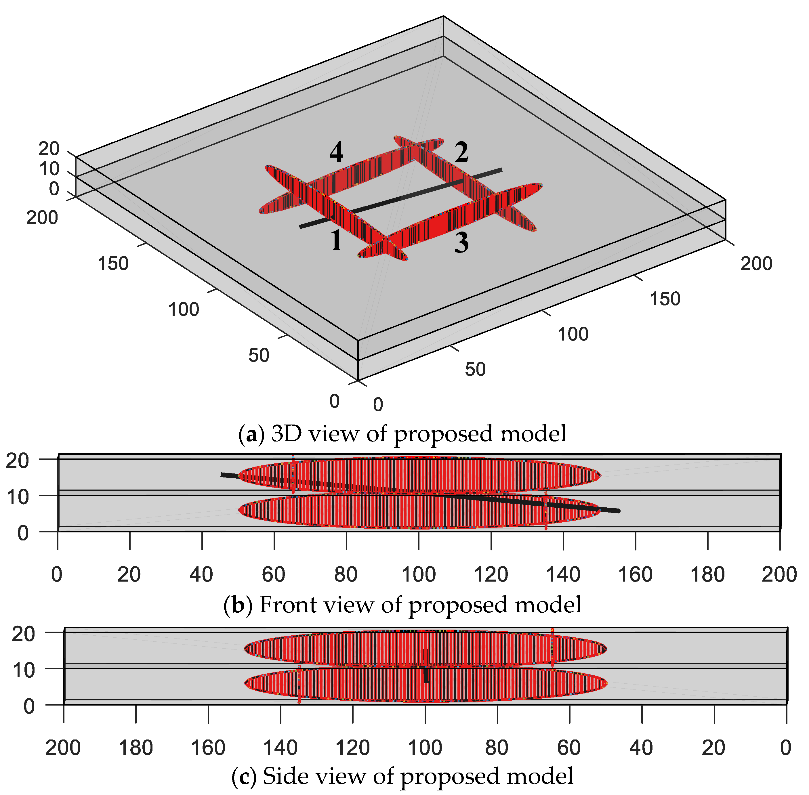
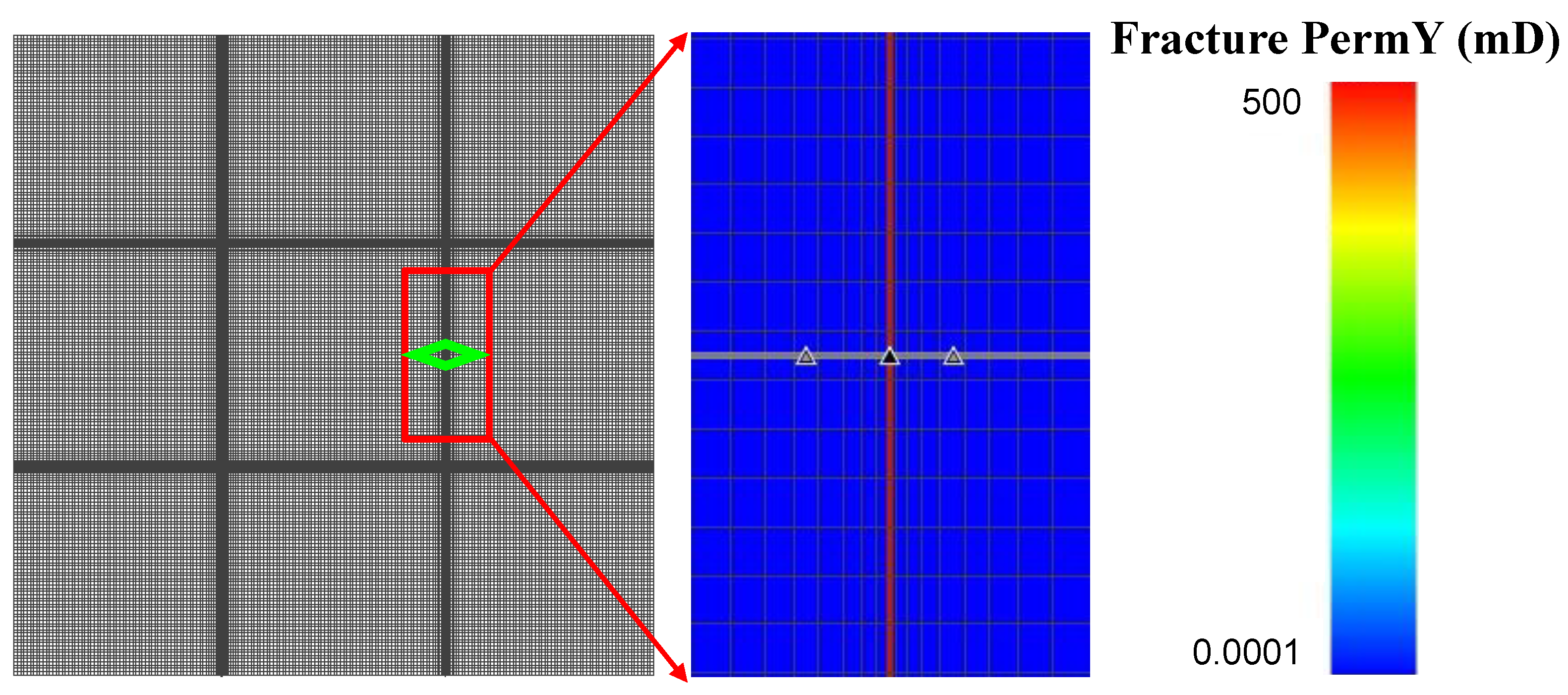
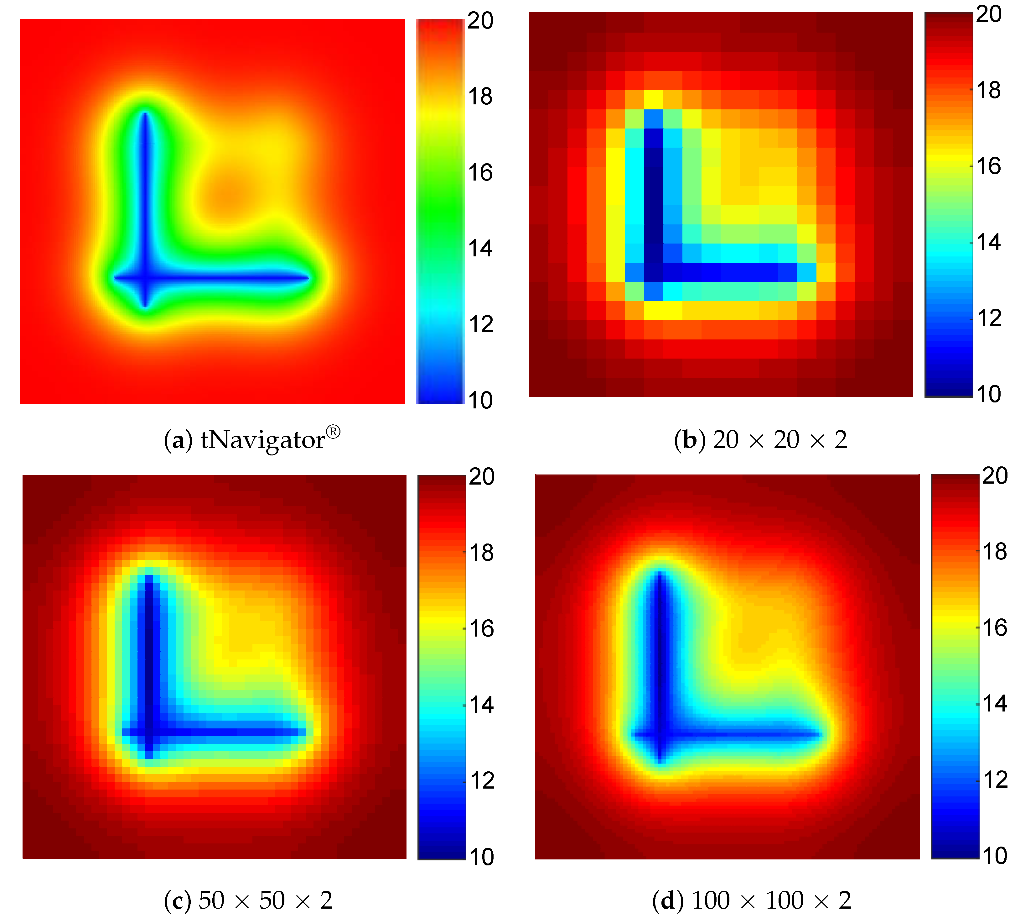
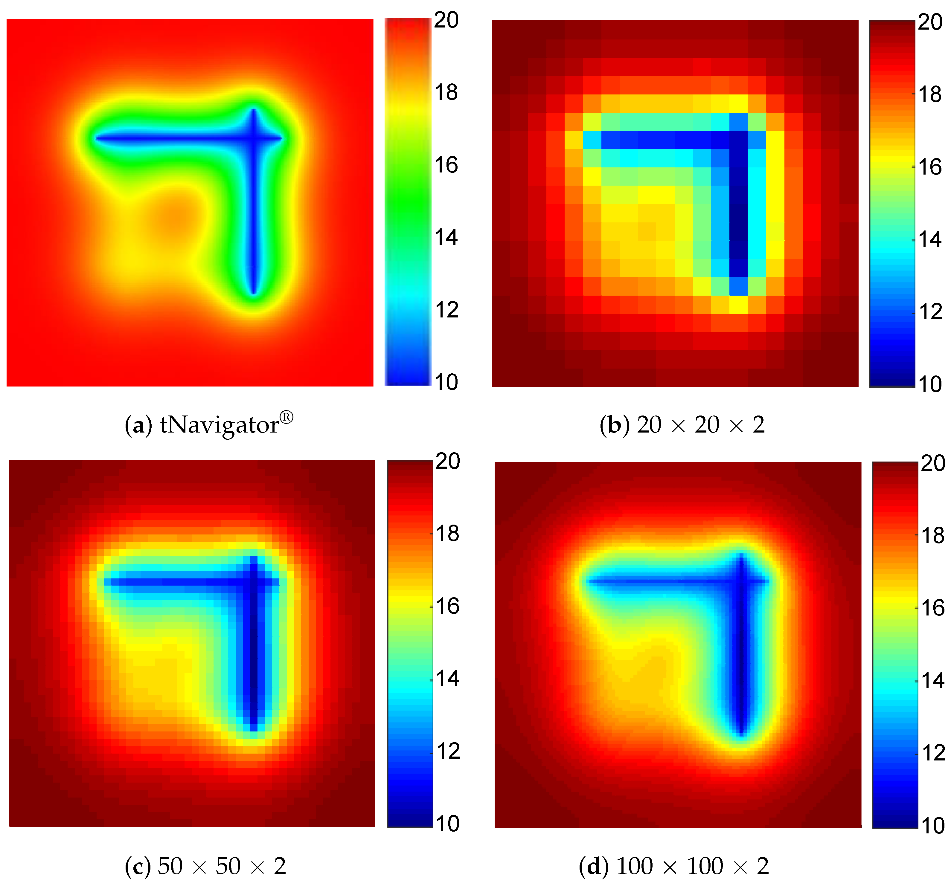
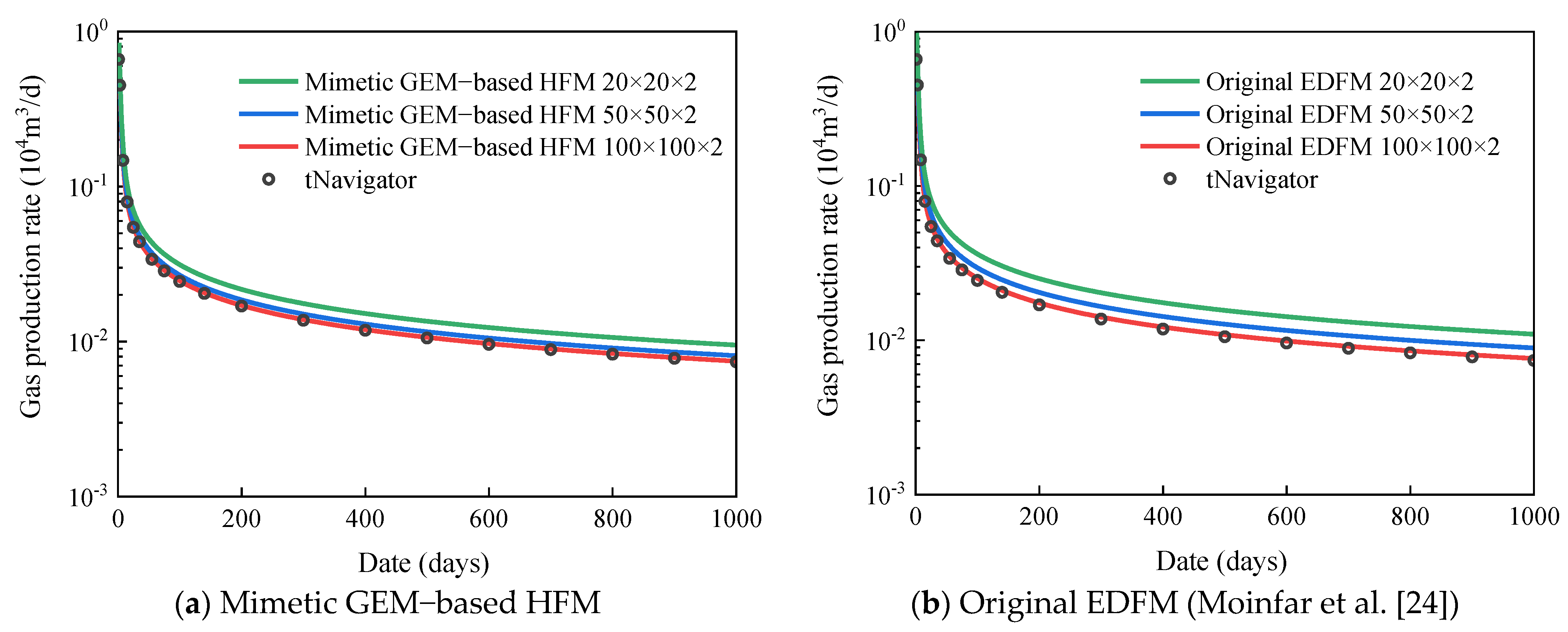
3.1. Simulation for Embedded Macro-Fractures

The accuracy of proposed three-dimensional embedded ellipsoidal macro-fracture model is compared with a commercial advanced reservoir-simulation software named tNavigator^® developed by a group named rock flow dynamics (RFD), which has become the industry standard. The induced fractures and natural fractures are removed in this comparison. The purpose of the first example is to verify whether the proposed method can generate arbitrary-placed fractures in different layers to achieve 3D reservoir simulation. The fractures are vertical in this case because it is relatively difficult for commercial software to characterize the fractures with arbitrary dip angles. A fractured inclined-well modeled by proposed method and the 3D reservoir model with fracture elements and the inclined wellbore is shown in Figure 6. The reservoir dimensions are 200 × 200 × 20 m and have two layers. The different grid divisions, such as 20 × 20 × 2, 50 × 50 × 2, and 100 × 100 × 2, are used to test the mesh sensitivity of proposed model. Modeling parameters of reservoir and fluid are shown in

Table 1. Modeling parameters of reservoir and fluid.

Properties	Value	Properties	Value
Initial reservoir pressure, MPa	20	Gas density, fraction	0.72
Gas viscosity, mPa·s	0.01	Gas Z-factor, fraction	0.8
Langmuir pressure, MPa	4.8	Langmuir volume, m3/kg	4 × 10−3
Matrix density, kg/m3	2400	Matrix compressibility, MPa−1	1.07 × 10−4
Matrix porosity, fraction	0.1	Matrix permeability, mD	1 × 10−4
Fracture compressibility, MPa−1	1 × 10−2	Fracture permeability, mD	500

. There are four fractures, of which No. 1 and No. 3 are in the top layer, and No. 2 and No. 4 are in the bottom layer. The fracture parameters in example 1 are shown in

Table 2. Fracture parameters in example 1.

Number	Reference Point Coordinates	Azimuth Angle, °	Fracture Length, m	Fracture Height, m
1	(65, 100, 15)	90	100	10
2	(135, 100, 5)	90	100	10
3	(100, 65, 15)	180	100	10
4	(100, 135, 5)	180	100	10

. The technology of local grid refinement (LGR) is used to describe the fractures and the schematic of the grid system with LGR for the commercial simulator tNavigator^® is illustrated as Figure 7. The fractured inclined-well is producing at a constant BHP of 10 MPa and the simulation time for production is 1000 days. The comparison of pressure profiles for different layers between tNavigator^® and our model on the 1000th day is illustrated in Figure 8 and Figure 9, and the computational results of the two models are very similar. Figure 10 shows the difference of the gas production rate of three simulators (tNavigator^®, original EDFM, and mimetic GEM-based HFM) simulating over 1000 days, in which the effect of mesh sensitivity is tested in this comparison between the original model and modified model. The comparison of grid number and average relative errors are shown in

Table 3. Comparison of grid number and average relative errors.

Modeling Simulator	Number of Grids	Average Relative Errors, %
tNavigator® (220 × 220 × 2)	96,800	-
Original EDFM (20 × 20 × 2)	800	48.11
Original EDFM (50 × 50 × 2)	5000	21.81
Original EDFM (100 × 100 × 2)	20,000	4.16
Proposed model (20 × 20 × 2)	800	28.24
Proposed model (50 × 50 × 2)	5000	9.59
Proposed model (100 × 100 × 2)	20,000	1.08

. The result of simulators under this benchmark proves that the modified model has higher precision and higher robustness than previous EDFMs that adopt a linear steady assumption. The HFM based on mimetic GEM achieves an accurate calculate of matrix–fracture mass transfer. Consequently, the mesh convergence and accuracy of proposed method in this paper are validated when we take the solution of tNavigator^® as the exact solution.

In the prior example, the arbitrary-placed fractures in different layers are modeled by proposed approach, and the results are proved to be accurate by comparing with LGR that is represented by a commercial simulator tNavigator^®. The second numerical example is supplemented to discuss the availability of the characterization model of inclined elliptic fractures. Figure 11 shows the 3D view and overhead view of the reservoir with a three-stage fractured horizontal well, in which it is obvious that some of the fractures are inclined and arbitrarily distributed. The reservoir size is 1000 × 500 × 40 m and has four layers. The modeling parameters of reservoir and fluid are the same as in Table 1. There are seven fractures with different azimuth angles, dip angles, lengths, heights, and the reference center point coordinates of fractures in this example are shown in

Table 4. Fracture parameters in example 2.

Number	Center Point Coordinates	Azimuth Angle, °	Dip Angle, °	Fracture Length, m	Fracture Height, m
1	(305, 255, 20)	70	95	300	30
2	(505, 255, 20)	93	70	280	30
3	(705, 255, 20)	87	75	295	30
4	(305, 195, 20)	15	60	200	25
5	(335, 345, 20)	30	90	180	25
6	(515, 315, 20)	20	88	190	20
7	(695, 155, 20)	20	90	210	15

. Fractures No. 1, No. 2, No. 3, No. 4, and No. 5 are completely penetrating the 2nd layer and 3rd layer, and partly penetrating the 1st layer and 4th layer in varying degrees. By contrast, the fracture No. 6 and No. 7 are not penetrating the top layer and the bottom layer because of the self-height and inclination degree. The constant BHP of 10 MPa. The production time is 1000 days, and the comparison of pressure profiles for different layers on the 1000th day is shown in Figure 12. It can be seen from this example that the proposed model can be adaptive to arbitrary inclined fracture with an elliptic shape. Compared with previous EDFMs, this is an innovative characterization method for ellipsoidal-shaped fractures in 3D-reservoir. Compared with the simulator tNavigator^®, the presented approach can handle not only arbitrary-placed fractures but also characterize the fractures with arbitrary dip angles.

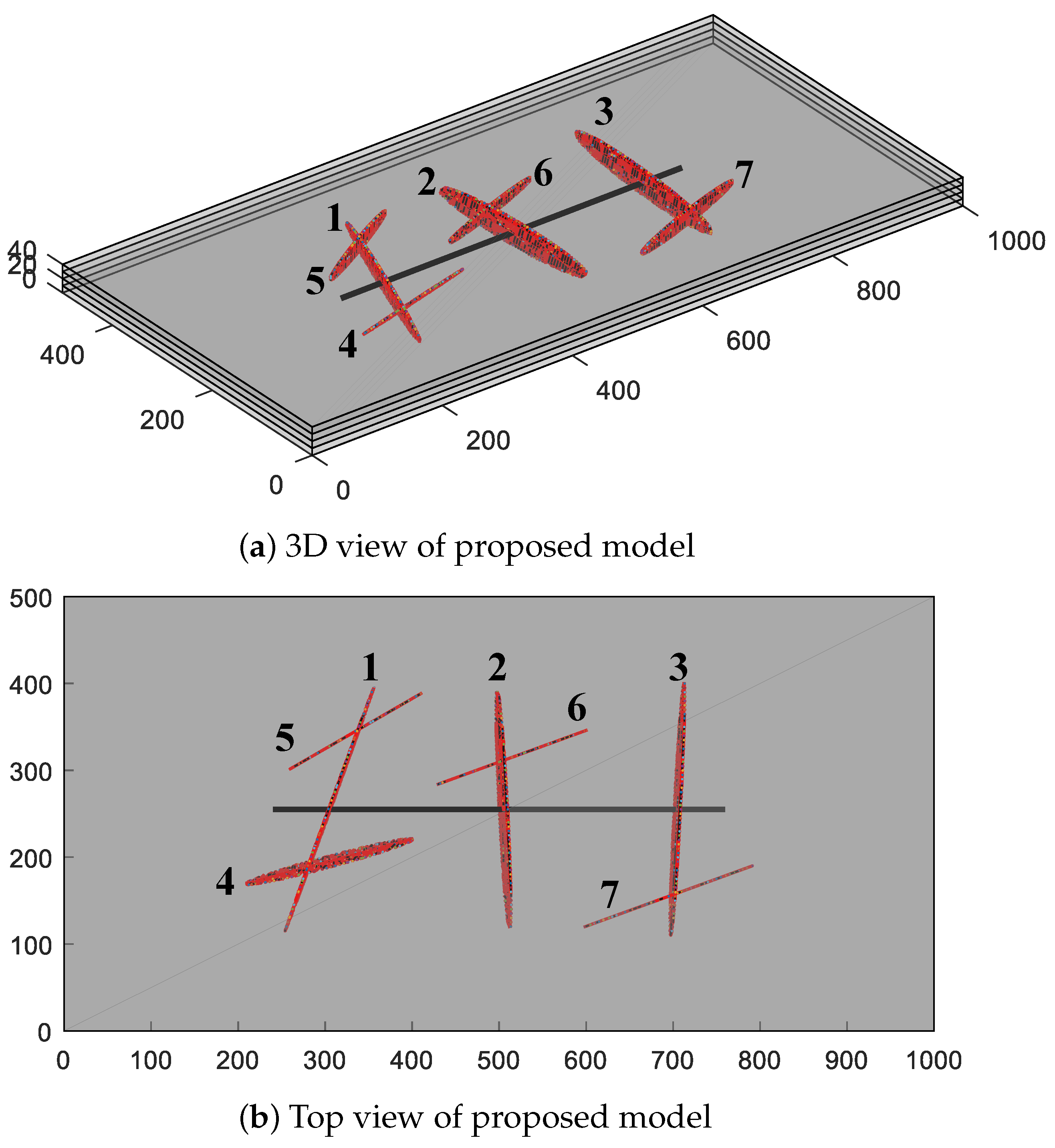
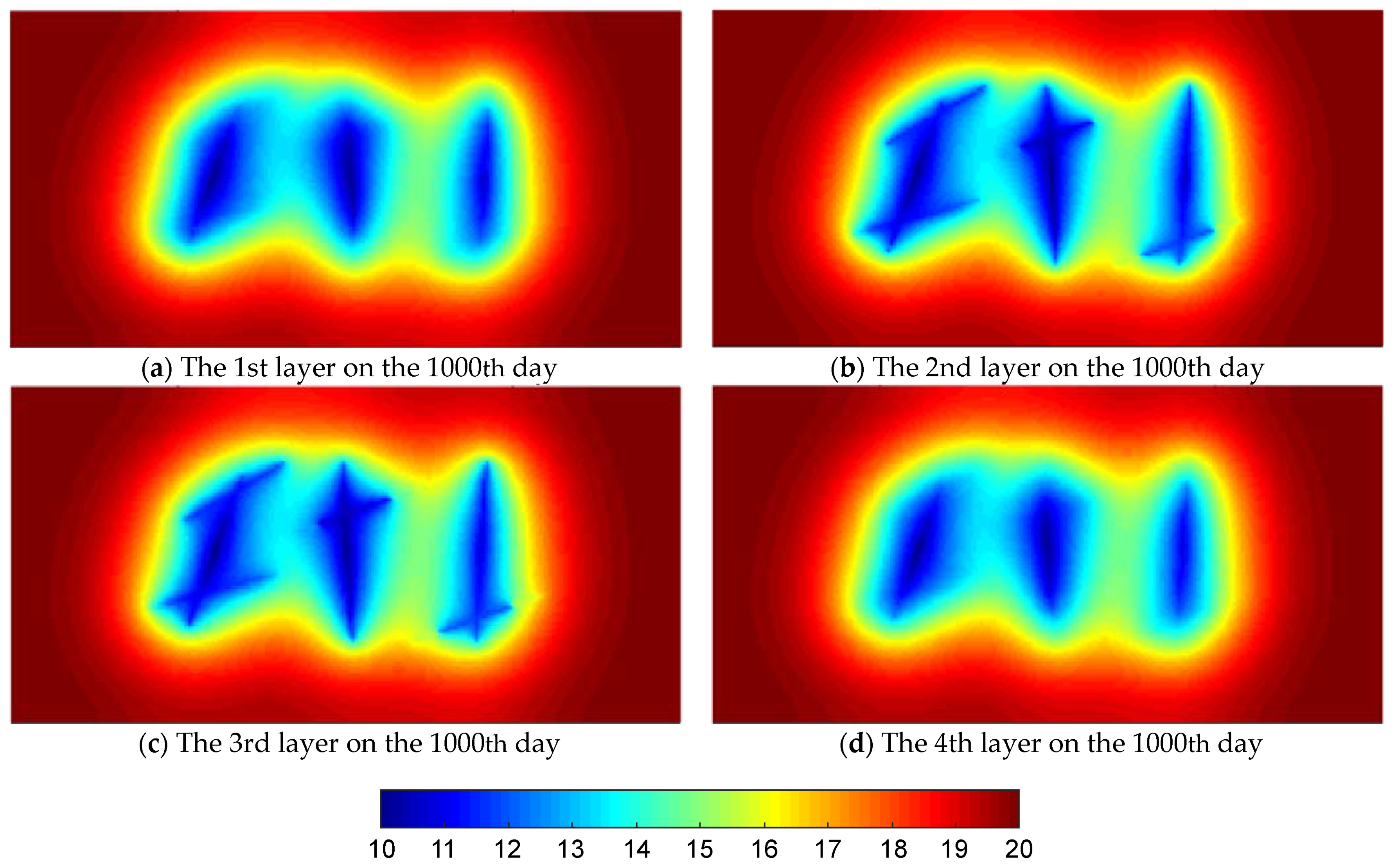
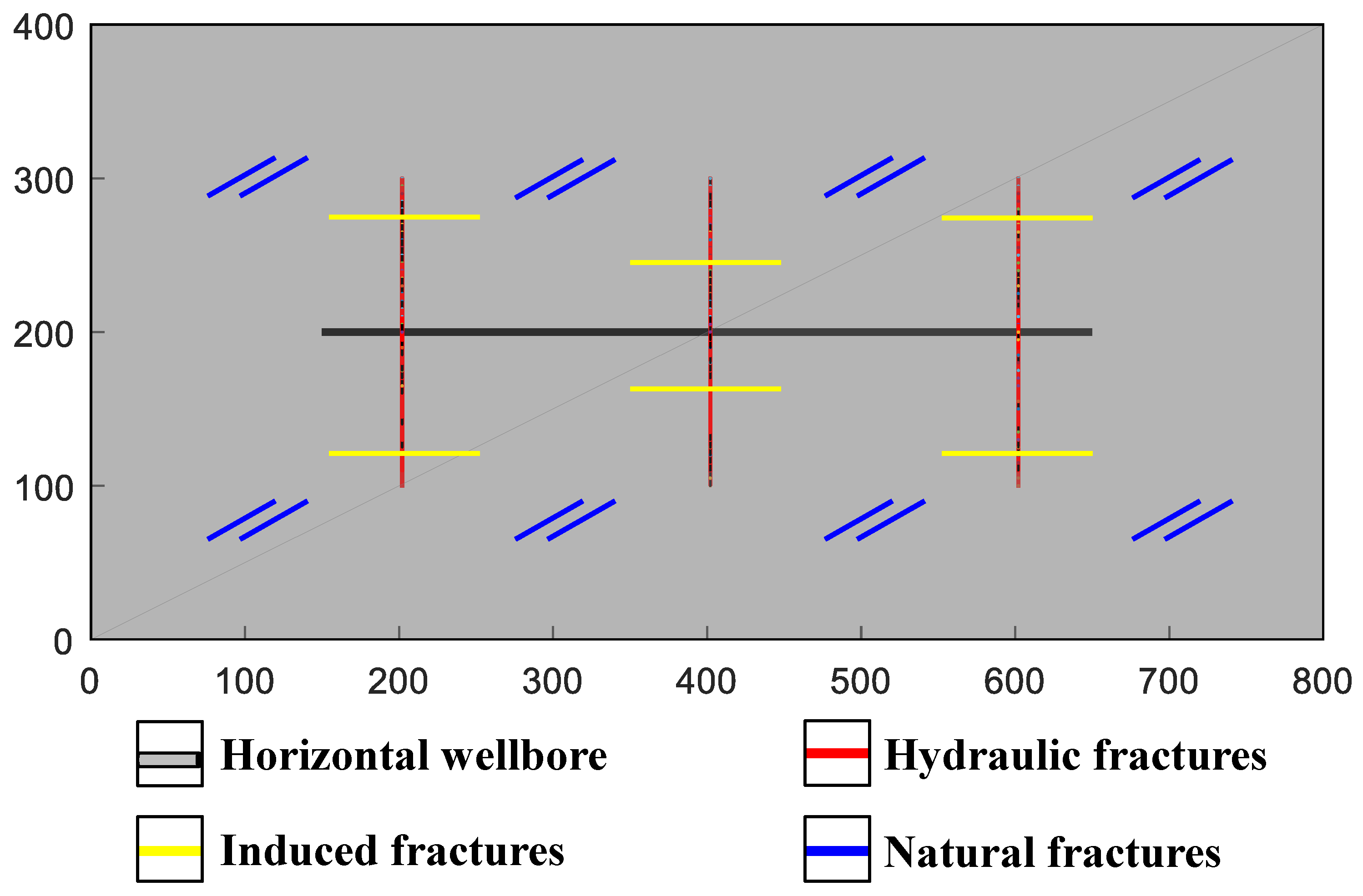
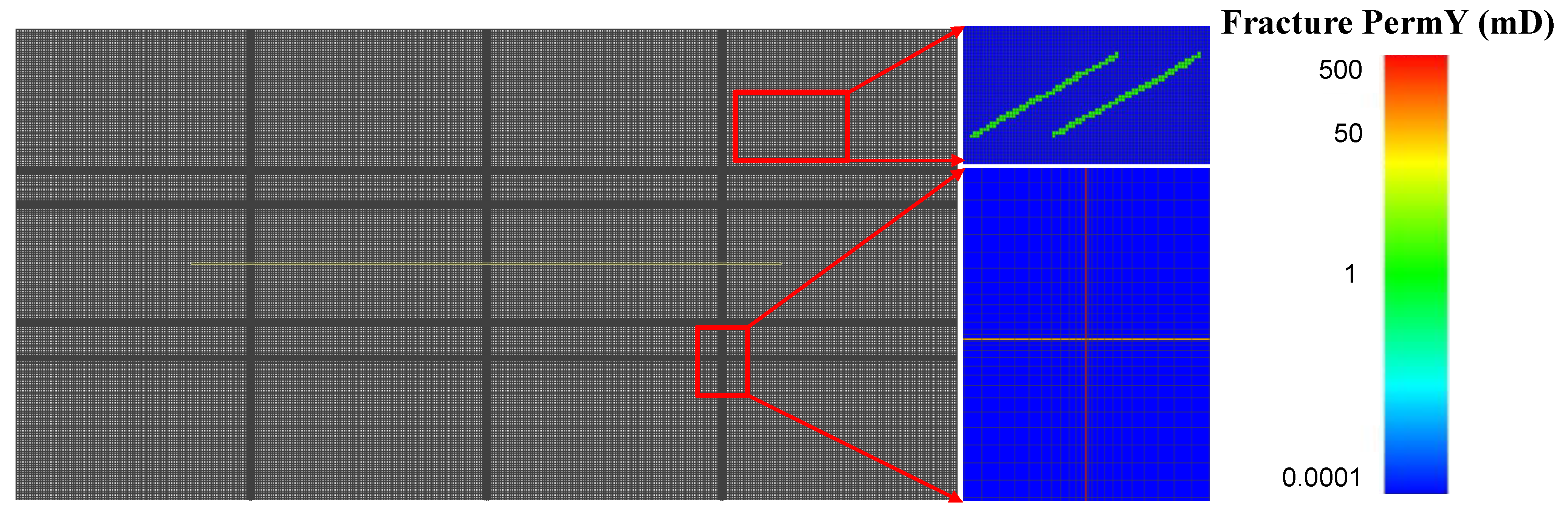
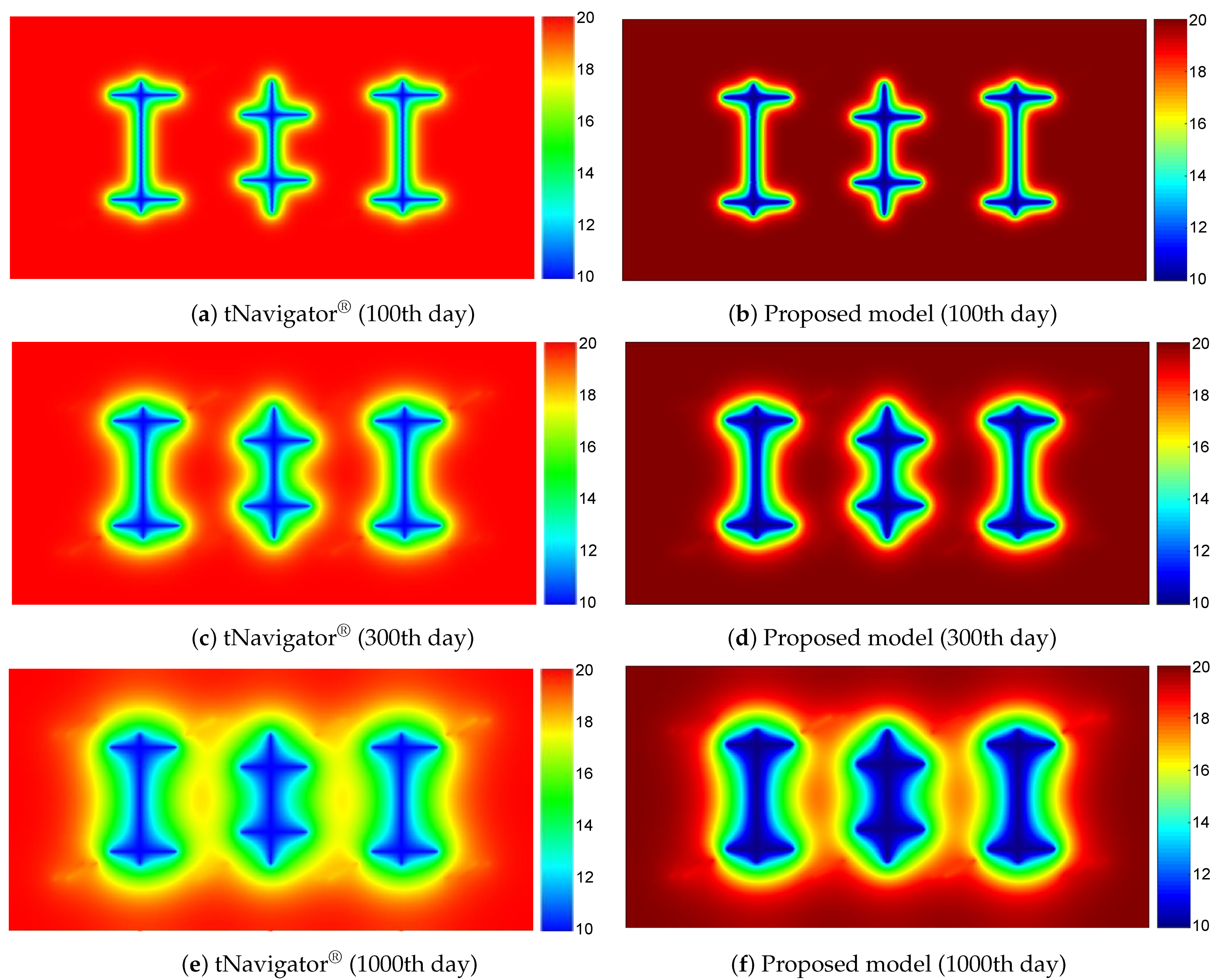
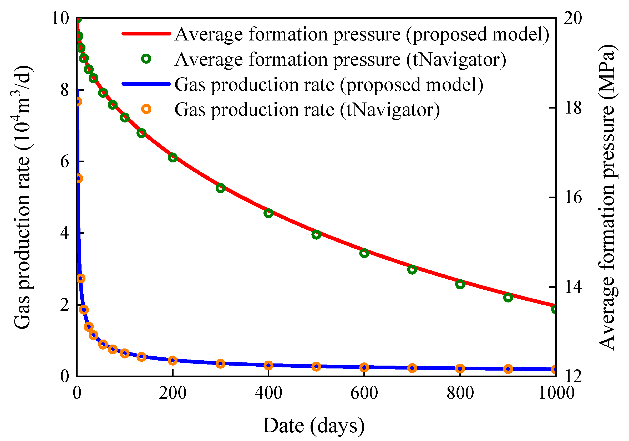
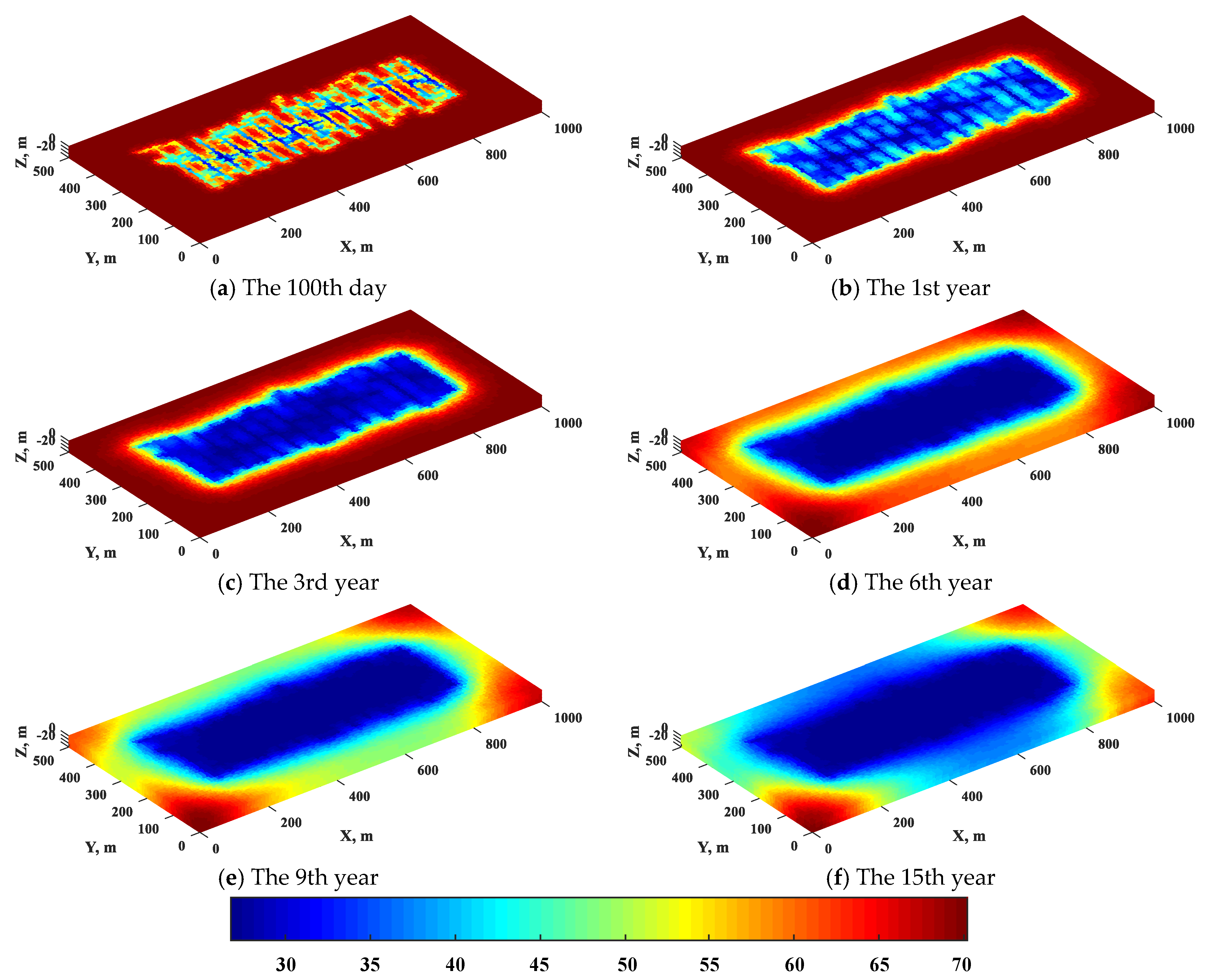
3.2. Simulation for Multi-Scale CFNs

A staged-fractured horizontal well with a set of multi-scale CFNs is designed by proposed hybrid model as shown in Figure 13. The accuracy and stability of proposed model are compared and verified by commercial simulator tNavigator^®. The reservoir dimensions are 800 × 400 × 10 m and only have one layer. The modeling parameters of the reservoir and fluid are the same as in Table 1. To saving the computing cost, all of the fractures are completely penetrating the reservoir and without any arbitrary dip angles. The fracture parameters are shown in

Table 5. Fracture parameters of multi-scale CFNs.

Fracture Type	Azimuth Angle, °	Fracture Length, m	Fracture Aperture, mm	Permeability, mD
Hydraulic fracture	90	200	1	500
Induced fracture	180	100	0.1	50
Natural fracture	30	50	0.01	1

and the noticeable differences between different scale fractures are length, aperture, and azimuth degree. The multi-scale CFNs are modeled by tNavigator^® and illustrated in Figure 14. In tNavigator^®, the LGR method and DPDK model are used for modeling the hydraulic fractures and induced fractures separately, and the matrix enhancement equivalent approach is adopted for micro-scale fractures. In this case, the two models keep the same size of grid-block, but the number of fracture elements in tNavigator^® is more than that in our model and this is caused by LGR. The production time is 1000 days under a constant BHP of 10 MPa. The comparison of pressure profiles for multi-scale CFNs in different periods is shown in Figure 15, the comparison of production dynamics calculated by two simulators over 1000 days is Figure 16, and the comparison of grid number and average relative errors for two simulators is

Table 6. Comparison of grid number and simulation time for two simulators.

Modeling Simulator	Number of Grids	Average Relative Errors, %
tNavigator® (830 × 440 × 1)	365,200	-
Proposed hybrid model (800 × 400 × 1)	320,000	4.09

. The simulation results showed a good agreement for pressure profiles, daily production curve, and the average reservoir pressure curve of two simulators on the 1000 days. The results within a reasonable error range indicate the high accuracy of the proposed hybrid model.

4. Application Case

In this section, we give a typical field case that simulates a multi-stage fractured horizontal well to discuss the practicability of proposed model. The studied shale gas well is located in the Sichuan Basin of southwestern China. A certain scale of natural fractures is developed in this shale formation and all the data come from this area.

Table 7. Modeling parameters of shale reservoir and fluids.

Properties	Value	Properties	Value
Reservoir volume, m	1000 × 500 × 30	Grid number	100 × 50 × 3
Depth, m	2800	Initial reservoir pressure, MPa	69
Horizontal wellbore length, m	805	Well radius, m	0.18
Skin factor	0.1	Gas density, fraction	0.72
Gas viscosity, mPa·s	0.01	Gas Z-factor, fraction	0.8
Langmuir pressure, MPa	4.8	Langmuir volume, m3/kg	4 × 10−3
Matrix density, kg/m3	2400	Matrix compressibility, MPa−1	1.07 × 10−4
Matrix porosity, fraction	0.1	Matrix permeability, mD	6 × 10−4
Fracture number	15	Fracture spacing, m	50
Fracture half-length, m	125	Fracture compressibility, MPa−1	1 × 10−2
Macro-fracture aperture, mm	1	Macro-fracture permeability, mD	500
Induced-fracture aperture, mm	0.1	Induced-fracture permeability, mD	50
Micro-fracture aperture, mm	0.01	Micro-fracture permeability, mD	1

shows the modeling parameters of reservoir and fluids, such as rock, fracture, and gas-phase properties.The testing results of water saturation show that the irreducible water saturation of shale rock is 28.1~40.2%, with an average of 34.2%, which is ultra-low water saturation. Additionally, the volume of adsorbed gas in shale core accounts for 27.8% of the total gas volume according to the experiment results.

Modeling for multi-scale fractures is shown in Figure 17. Firstly, all hydraulic macro-fractures are assumed to be evenly distributed on the horizontal section. The basic model of 3D reservoirs with the embedded macro-fractures and the horizontal wellbore is modeled in Figure 17a. The induced fractures and natural micro-fractures are modeled with the multi-stochastical simulation method according to the actual situation of shale gas reservoirs. Their corresponding 3D spatial position coordinates are stochastically generated by the Monte Carlo method [47] and generated in the formation. The difference between them is that the induced fractures only exist in the SRV, while the natural fractures exist in whole reservoirs. The strike of these fractures is determined by multiple-point geostatistics and the trend of minimum horizontal principal stress is taken as an average value with a standard deviation is 20°. The total number of meso-scale induced fractures is 70 and its length is determined by Boolean random simulation with an average value of 35 m and the standard deviation of 10 m. Similarly, the total number of natural micro-fractures is 300 and its average value of length is 15m with a standard deviation of 5 m. The basic model of induced fractures is shown in Figure 17b. and the natural micro-fractures modeling is shown in Figure 17c. The next step is to find the matrix grid where the meso-scale and micro-scale fractures are located and treat them with their respective equivalent methods. Lastly, combining the three models in Figure 17a, Figure 17b and Figure 17c to obtain a coupled triple-porosity triple-permeability hybrid model for simulating the multiscale fracture networks. The reservoir pressure distribution map at the different years, in this case, is illustrated in Figure 18.

Figure 19 shows the simulation results of formation pressure and the gas production rate. At present, this studied fractured horizontal well in Sichuan has been in production for about six years. Comparing the production performance data calculated by proposed model with the field production data, it can be proved that the trend of productivity is highly consistent and the errors were acceptable. The above comparison results explain that the proposed model has high reliability. The development of shale gas reservoirs is dominated by fracture-controlled resources. Therefore, the permeability of each scale fracture is an important evaluation parameter, which directly influences the gas recovery.

5. Conclusions

A hybrid hierarchical fracture modeling framework is proposed in this paper to match the multiscale CFNs and benchmarked with tNavigator^®. The results prove that the proposed model has high precision and high robustness. The proposed hybrid model was applied for simulation of a typical well in Sichuan shale, indicating that the proposed method can provide theoretical guidance for productivity forecasting and optimization. The simulation results show that the multiscale CFNs is an essential consideration affecting the production of gas wells. Generally, the enlightenment for engineering technicians mainly includes two aspects. Firstly, it is very important to establish high-conductivity macro-fractures as preferential channeling, and secondly, it is necessary to increase the area and utilization rate of SRV.

References

1. Wei, W.; Xia, Y. Geometrical, fractal and hydraulic properties of fractured reservoirs: A mini-review. Adv. Geo-Energy Res. 2017, 1, 31–38. [Google Scholar] [CrossRef] [Green Version]
2. Ebrahim, G.; Hassan, D. The fate of fracturing water: A field and simulation study. Fuel 2016, 163, 282–294. [Google Scholar]
3. Jia, P.; Cheng, L.-S.; Huang, S.-J. Transient behavior of complex fracture networks. J. Pet. Sci. Eng. 2015, 132, 1–17. [Google Scholar] [CrossRef]
4. Medeiros, F.; Ozkan, E.; Kazemi, H. A semianalytical approach to model pressure transients in heterogeneous reservoirs. SPE Reserv. Eval. Eng. 2010, 13, 341–358. [Google Scholar] [CrossRef]
5. Shakiba, M.; Cavalcante, A.; Sepehrnoori, K. Using embedded discrete fracture model (EDFM) in numerical simulation of complex hydraulic fracture networks calibrated by microseismic monitoring data. J. Nat. Gas Sci. Eng. 2018, 55, 495–507. [Google Scholar] [CrossRef]
6. Wu, Y.-H.; Cheng, L.-S.; Killough, J.E. Integrated characterization of the fracture network in fractured shale gas reservoirs—Stochastic fracture modeling, simulation and assisted history matching. In Proceedings of the SPE Annual Technical Conference and Exhibition, Calgary, AB, Canada, 30 September–2 October 2019. [Google Scholar]
7. Sun, J.; Niu, G.; Schechter, D. Numerical simulation of stochastically-generated complex fracture networks byutilizing core and microseismic data for hydraulically fractured horizontal wells in unconventional reservoirs—A field case study. In Proceedings of the SPE Eastern Regional Meeting, Canton, OH, USA, 13–15 September 2016. [Google Scholar]
8. Obembe, A.D.; Hossain, M.E. A new pseudosteady triple-porosity model for naturally fractured shale gas reservoir. In Proceedings of the SPE Annual Technical Conference and Exhibition, Houston, TX, USA, 28–30 September 2015. [Google Scholar]
9. Jiang, J.; Younis, R. A multimechanistic multicontinuum model for simulating shale gas reservoir with complex fractured system. Fuel 2015, 161, 333–344. [Google Scholar] [CrossRef]
10. Zhang, T.; Li, Z.; Adenutsi, C.D.; Lai, F. A new model for calculating permeability of natural fractures in dual-porosity reservoir. Adv. Geo-Energy Res. 2017, 1, 86–92. [Google Scholar] [CrossRef] [Green Version]
11. Barenblatt, G.; Zheltov, I. Basic flow equations for homogeneous fluids in naturally fractured rocks. Doklady Akad. Nauk. 1960, 13, 245–255. [Google Scholar]
12. Warren, J.; Root, P. The behavior of naturally fractured reservoirs. SPE J. 1963, 3, 245–255. [Google Scholar] [CrossRef] [Green Version]
13. Pruess, K.; Narasimhan, T. On fluid reserves and the production of superheated steam from fractured, vapor-dominated geothermal reservoirs. J. Geophys. Res. 1982, 87, 9329–9339. [Google Scholar] [CrossRef]
14. Pruess, K.; Narasimhan, T. A practical method for modeling fluid and heat flow in fractured porous media. SPE J. 1985, 25, 14–26. [Google Scholar] [CrossRef] [Green Version]
15. Wu, Y.; Pruess, K. A multiple-porosity method for simulation of naturally fractured petroleum reservoirs. SPE Reserv. Eng. 1988, 3, 327–336. [Google Scholar] [CrossRef] [Green Version]
16. Blaskovich, F.; Cain, G.; Webb, S. A multicomponent isothermal system for efficient reservoir simulation. In Proceedings of the Middle East Oil Technical Conference and Exhibition, Manama, Bahrain, 14–17 March 1983. [Google Scholar]
17. Hill, A.; Thomas, G. A new approach for simulating complex fractured reservoirs. In Proceedings of the Middle East Oil Technical Conference and Exhibition, Manama, Bahrain, 11–14 March 1985. [Google Scholar]
18. Moinfar, A.; Narr, W.; Hui, M. Comparison of discrete-fracture and dual-permeability models for multiphase flow in naturally fractured reservoirs. In Proceedings of the SPE Reservoir Simulation Symposium, Woodlands, TX, USA, 21–23 February 2011. [Google Scholar]
19. Noorishad, J.; Mehran, M. An upstream finite element method for solution of transient transport equation in fractured porous media. Water Resour. Res. 1982, 18, 588–596. [Google Scholar] [CrossRef] [Green Version]
20. Kim, J.G.; Deo, M.D. Finite element discrete-fracture model for multiphase flow in porous media. AIChE J. 2000, 46, 1120–1130. [Google Scholar] [CrossRef]
21. Wang, Y.; Shahvali, M. Discrete fracture modeling using Centroidal Voronoi grid for simulation of shale gas plays with coupled nonlinear physics. Fuel 2016, 163, 65–73. [Google Scholar] [CrossRef]
22. Lee, S.H.; Lough, M.F.; Jensen, C.L. Hierarchical modeling of flow in naturally fractured formations with multiple length scales. Water Resour. Res. 2001, 37, 443–498. [Google Scholar] [CrossRef]
23. Li, L.; Lee, S.H. Efficient field-scale simulation of black oil in a naturally fractured reservoir through discrete fracture networks and homogenized media. SPE Reserv. Eval. Eng. 2008, 11, 750–758. [Google Scholar] [CrossRef]
24. Moinfar, A.; Varavei, A.; Sepehrnoori, K. Development of an efficient embedded discrete fracture model for 3D compositional reservoir simulation in fractured reservoirs. SPE J. 2014, 19, 289–303. [Google Scholar] [CrossRef] [Green Version]
25. Snow, D.T. Rock fracture spacings, openings, and porosities closure. J. Soil Mech. Found. Div. 1968, 94, 73–92. [Google Scholar] [CrossRef]
26. Matthäi, S.; Mezentsev, A.; Belayneh, M. Control-volume finite-element two-phase flow experiments with fractured rock represented by unstructured 3D hybrid meshes. In Proceedings of the SPE Reservoir Simulation Symposium, Woodlands, TX, USA, 31 January–2 February 2005. [Google Scholar]
27. Reichenberger, V.; Jakobs, H.; Bastian, P. A mixed-dimensional finite volume method for two-phase flow in fractured porous media. Adv. Water Resour. 2006, 29, 1020–1056. [Google Scholar] [CrossRef]
28. Monteagudo, J.; Firoozabadi, A. Control-volume method for numerical simulation of two-phase immiscible flow in two and three-dimensional discrete fractured media. Adv. Water Resour. 2004, 40, 7405. [Google Scholar] [CrossRef] [Green Version]
29. Karimi-Fard, M.; Durlofsky, L.J.; Aziz, K. An efficient discrete-fracture model applicable for general-purpose reservoir simulators. SPE J. 2004, 9, 227–260. [Google Scholar] [CrossRef]
30. Hoteit, H.; Firoozabadi, A. An efficient numerical model for incompressible two-phase flow in fractured media. Adv. Water Resour. 2008, 31, 891–905. [Google Scholar] [CrossRef]
31. Cockburn, B.; Karniadakis, G.E.; Shu, C. The development of discontinuous Galerkin methods. In Discontinuous Galerkin Methods; Springer: Berlin/Heidelberg, Germany, 2000; pp. 3–50. [Google Scholar]
32. Su, H.; Lei, Z.; Li, J. An effective numerical simulation model of multi-scale fractures in reservoir. Acta Pet. Sin. 2019, 40, 587–593. [Google Scholar]
33. Panfili, P.; Cominelli, A. Simulation of miscible gas injection in a fractured carbonate reservoir using an embedded discrete fracture model. In Proceedings of the Abu Dhabi International Petroleum Exhibition and Conference, Abu Dhabi, United Arab Emirates, 10–13 November 2014. [Google Scholar]
34. Fang, S.-D.; Cheng, L.-S.; Ayala, L.F. A coupled boundary element and finite element method for the analysis of flow through fractured porous media. J. Pet. Sci. Eng. 2017, 152, 375–390. [Google Scholar] [CrossRef]
35. Cao, R.-Y.; Fang, S.-D.; Jia, P. An efficient embedded discrete-fracture model for 2D anisotropic reservoir simulation. J. Pet. Sci. Eng. 2018, 174, 115–130. [Google Scholar] [CrossRef]
36. Rao, X.; Cheng, L.-S.; Cao, R.-Y. An efficient three-dimensional embedded discrete fracture model for production simulation of multi-stage fractured horizontal well. Eng. Anal. Bound. Elem. 2019, 106, 473–492. [Google Scholar] [CrossRef]
37. Saidi, A. Simulation of naturally fractured reservoirs. In Proceedings of the SPE Reservoir Simulation Symposium, San Francisco, CA, USA, 15–18 November 1983. [Google Scholar]
38. Tene, M.; Bosma, S.B.; Al Kobaisi, M.S.; Hajibeygi, H. Projection-based embedded discrete fracture model (pEDFM). Adv. Water Resour. 2017, 105, 205–221. [Google Scholar] [CrossRef]
39. Nejati, M.; Paluszny, A.; Zimmerman, R.W. A finite element framework for modeling internal frictional contact in three-dimensional fractured media using unstructured tetrahedral meshes. Comput. Methods Appl. Mech. Eng. 2016, 306, 123–150. [Google Scholar] [CrossRef] [Green Version]
40. Zhang, J.; Huang, S.; Cheng, L.; Xu, W.; Liu, H.; Yang, Y.; Xue, Y. Effect of flow mechanism with multi-nonlinearity on production of shale gas. J. Nat. Gas Sci. Eng. 2015, 24, 291–301. [Google Scholar] [CrossRef]
41. Yang, Z.; Wang, W.; Dong, M.; Wang, J.; Li, Y.; Gong, H.; Sang, Q. A model of dynamic adsorption–diffusion for modeling gas transport and storage in shale. Fuel 2016, 173, 115–128. [Google Scholar] [CrossRef]
42. Du, X.; Cheng, L.; Liu, Y.; Rao, X.; Ma, M.; Cao, R.; Zhou, J. Application of 3D embedded discrete fracture model for simulating CO2-EOR and geological storage in fractured reservoirs. IOP Conf. Ser. Earth Environ. Sci. 2020, 467, 012013. [Google Scholar] [CrossRef]
43. Hajibeygi, H.; Karvounis, D.; Jenny, P. A hierarchical fracture model for the iterative multiscale finite volume method. J. Comput. Phys. 2011, 230, 8729–8743. [Google Scholar] [CrossRef]
44. Yan, X.; Huang, Z.; Yao, J.; Li, Y.; Fan, D. An efficient embedded discrete fracture model based on mimetic finite difference method. J. Pet. Sci. Eng. 2016, 145, 11–21. [Google Scholar] [CrossRef]
45. Rao, X.; Cheng, L.-S.; Cao, R.-Y. A mimetic Green element method. Eng. Anal. Bound. Elem. 2019, 99, 206–221. [Google Scholar] [CrossRef]
46. Karimi, F.M.; Firoozabadi, A. Numerical simulation of water injection in fractured media using the discrete-fracture model and the Galerkin method. SPE Reserv. Eval. Eng. 2003, 6, 117–126. [Google Scholar] [CrossRef]
47. Ritchie, D.; Mildenhall, B.; Goodman, N.D. Controlling procedural modeling programs with stochastically-ordered sequential Monte Carlo. ACM Trans. Graph. 2015, 34, 105. [Google Scholar] [CrossRef]
Figure 1. Schematic plot of multiscale fractures distribution after hydraulic fracturing.
Energies 14 06354 g001
Figure 2. Schematic plot of ellipsoidal fracture model (modified from Rao et al. [36]).
Energies 14 06354 g002
Figure 3. The NNCs of EDFM simulation of macro-fracture.
Energies 14 06354 g003
Figure 4. Schematic plot of mimetic GEM-based HFM in rectangle grid.
Energies 14 06354 g004
Figure 5. Integrated workflow of multiscale CFNs modeling.
Energies 14 06354 g005
Figure 6. Modeling of 3D reservoir with fracture elements for example 1.
Energies 14 06354 g006
Figure 7. (Left) top view of the global grid configuration for macro-fracture. (Right) a view of locally interconnecting fractures and surrounding matrix blocks with permeability distribution in Y-direction. The distribution of permeability is also presented in the schematic by using various colors and the permeability distribution in X-direction is the same as that in Y-direction.
Energies 14 06354 g007
Figure 8. Comparison of pressure profiles for the top layer on the 1000th day.
Energies 14 06354 g008
Figure 9. Comparison of pressure profiles for the bottom layer on the 1000th day.
Energies 14 06354 g009
Figure 10. Comparison of the gas production rate of various simulators over 1000 days.
Energies 14 06354 g010
Figure 11. Modeling of 3D reservoir with fracture elements for example 2.
Energies 14 06354 g011
Figure 12. Comparison of pressure profiles for different layers on the 1000th day.
Energies 14 06354 g012
Figure 13. Modeling of the multi-scale CFNs.
Energies 14 06354 g013
Figure 14. (Left) top view of the global grid configuration for multi-scale CFNs. (Right) a view of locally interconnecting fractures and surrounding matrix grids with permeability distribution in Y-direction. The distribution of permeability is also presented in the schematic by various colors and the permeability distribution in X-direction is the same as that in Y-direction.
Energies 14 06354 g014
Figure 15. Comparison of pressure profiles for multi-scale CFNs in different periods.
Energies 14 06354 g015
Figure 16. Comparison of production dynamics calculated by two simulators over 1000 days.
Energies 14 06354 g016
Figure 17. Modeling for multi-scale fractures.
Energies 14 06354 g017
Figure 18. Pressure distribution map at the different years in this case.
Energies 14 06354 g018
Figure 19. Curves of formation pressure and gas production rate.
Energies 14 06354 g019