RES and ES Integration in Combination with Distribution Grid Development Using MILP


Institute of Mechatronics and Information Systems, Lodz University of Technology, 90-924 Lodz, Poland
Energies 2021, 14(2), 383; https://0-doi-org.brum.beds.ac.uk/10.3390/en14020383
Submission received: 14 December 2020
/
Revised: 6 January 2021
/
Accepted: 8 January 2021
/
Published: 12 January 2021
(This article belongs to the Special Issue Solar and Wind Power and Energy Forecasting)
Abstract
:In the paper, a new method of long-term planning of operation and development of the distribution system, taking into account operational aspects such as power flows, power losses, voltage levels, and energy balances, is presented. The developed method allows for the allocation and selection of the power of Renewable Energy Sources (RES), control of energy storage (ES), curtailing of RES production (EC), and the development of the distribution grid (GD). Different types of RES and loads are considered, represented by generation/demand profiles reflecting their typical operating conditions. RES allocation indicates the node in the distribution system and the power level for each type of RES that may be built. Energy storage (ES) allows generation to be transferred from the demand valley to the peak load. Curtailment of RES generation indicates the moment and level of power by which generation will be reduced, while the grid development (GD) determines between which network nodes a new power line should be built. All these activities allow to minimize the costs of planning work and development of the distribution system at a specific level of energy consumption from RES in the analyzed distribution system using a Mixed Integer-Linear Programming (MILP).
1. Introduction
In traditional power systems, electricity is generated in large generating units, and then, using the transmission system and distribution systems, it is sent to final customers. The European Union’s policy on renewable energy has resulted in a rapid increase in the number of Renewable Energy Sources (RES) connected to the distribution system. Most of these systems are not adapted to such a high share of renewable energy sources, whose energy production depend on atmospheric conditions and are difficult to predict in the long run. Problems with accurate forecasting the volume of electricity production from renewable energy sources and the nature of their work cause difficulties in the operation of power systems, which include high generation in the valley of the night demand curve and rapid changes in the level of electricity produced. The nature of RES work also results in network overload, mismatch between generation and demand, and an increase in the operating costs of the distribution system.
Research carried out as part of this work is devoted to developing a method of long-term work planning and development of the distribution system, taking into account operational aspects such as power flows, power losses, voltage levels, and energy balances. The developed method allows the allocation and selection of Renewable Energy Sources (RES), controlling energy storage (ES), reducing renewable energy production, and the development of a distribution network allowing for the addition of new installations. Various types of renewable energy sources and loads are considered, which are represented by generation/demand profiles reflecting the typical conditions of their operation.
The allocation of distributed energy sources has become a topic in recent years. According to the European Union policy, at least 20% of energy in the EU will come from Renewable Energy Sources (RES) by 2020 and 32% by 2030. Because most RES are connected to the distribution system, which was constructed for distribution energy only, this makes it necessary to develop new methods of work planning and development of these systems. In recent papers, we can distinguish a few groups differing of a used objective function. In [1], the ABC algorithm was used to minimize the power losses by determining the RES location, size, and power factor. Minimization of power losses was also used in [2,3]. In [2], authors utilized a genetic algorithm to allocate three types of distributed generation; they also used the daily profiles to characterize generation units and loads. In [3], PSO technique was used to find the optimal size of distributed generation (DG) at each bus. References [4,5] include power loss minimization and voltage improvement. Other papers used maximization of revenues of distribution companies [6,7] as an objective function. In both mentioned papers, objective function is achieved by optimal location of DGs, but they differ in used programming method (linear programming in [6] and dynamic programming in [7]). The other objective function (minimization of total costs) was presented in [8,9,10]. In [8], authors used a genetic algorithm to determine optimal location and capacity of DG over the number of planning years. In both [9,10], Mixed Integer-Linear Programming (MILP) is utilized to allocate DGs in microgrids [9] or radial networks [10].
Along with the increased installed capacity in renewable energy, whose nature of electricity generation is variable and difficult to predict, solutions are needed to ensure the security of the electricity supply. One of such solutions is the construction of energy storage (ES). In [11,12], only allocation of energy storage (ES) is considered. Two mentioned papers differ in the objective function (minimization of power losses [11] and minimization of costs [12]) and used method (ABC algorithm [11] and PSO [12]). Another approach was presented in [13,14,15,16], where ES and RES are allocated in parallel. In each of the papers, a different method was used: GA [13], LP [14], TLBO [15], and MILP [16]. In both papers [14,16], simulations were carried out for one year with one hourly step. Another solution presented in the literature is to use hydrogen storage technology [17].
Another method to reduce the negative impact of RES on the network is to limit their generation. Four different energy curtailment (EC) methods were considered. In the first case, the generation units are exclusive for the entire period when a violation of technical restrictions may occur [18]. In the second method, generation curtailment is about limiting generation to a constant level throughout the entire period when a violation of technical limitations may occur [19]. In [20], energy curtailment (EC) is adapted to technical constraints, which allows better adaptation of the generation to the constraints. The last paper presents a method of the proportional energy curtailment (EC) consisting of reducing the generation by a fixed factor for the entire analyzed period, even for periods when the limitations are not violated [21].
There are also works on optimizing the development of distribution and transmission systems. Reference [22] presents transmission network expansion planning. In [23,24], building of new lines and substations in the distribution system are considered. In both mentioned papers, minimization of investment and losses cost are implemented, but [23] used MILP and [24], GA. In [25], building of new lines and the allocation of RES is presented by using GA to achieve minimal investment and operational costs. More complex approaches are presented in [26,27,28] in which building of new lines, allocation of RES, and substations are considered. Three mentioned papers have the same objective function: minimization of investment and operational costs and differences that lie in the using method (MILP [26,27] and dynamic programming [28]). In another paper [29], the building of new lines and allocation of ES is considered.
Another way to improve the operation of the power system is to implement demand-side management (DSM) system [30]. The big advantage of these systems is the ability to control the load by consumers in response to the system’s demand, which significantly facilitates its operation. On the other hand, the allocation of new RES and ES allows for the development of energy clusters and allows to meet the EU requirements regarding the level of RES in the national mix.
Novelty of the Paper
Although there are many works devoted to the development of distribution systems, none of them show the method of comprehensive optimization using MILP and maintaining the technical standards of system operation and taking into account the variability of the generation of RES/loads within one year.
The originality of the method proposed in the article consists of the use of comprehensive optimization of distribution systems, consisting of the possibility of allocation and selection of Renewable Energy Sources (RES), allocation and selection of energy storage (ES) capacity, construction of new lines, and control of renewable energy using variable generation limitation. The optimization is carried out with the criterion of the lowest capital and operating costs, taking into account the variable nature of sources and loads for the long-term horizon.
2. Problem Formulation
The aim of this paper is to develop and simulate a new comprehensive method for optimizing medium voltage electricity distribution systems that minimizes the costs of their operation and development using Mixed-Integer Linear Programming and a bottom-up approach in which the main problem is reached through a detailed analysis of the model and assumptions.
The research problem considered in this paper includes optimization regarding three groups of objects connected to medium voltage distribution networks: construction of new generating units, construction of new energy reservoirs, network development by building new lines.
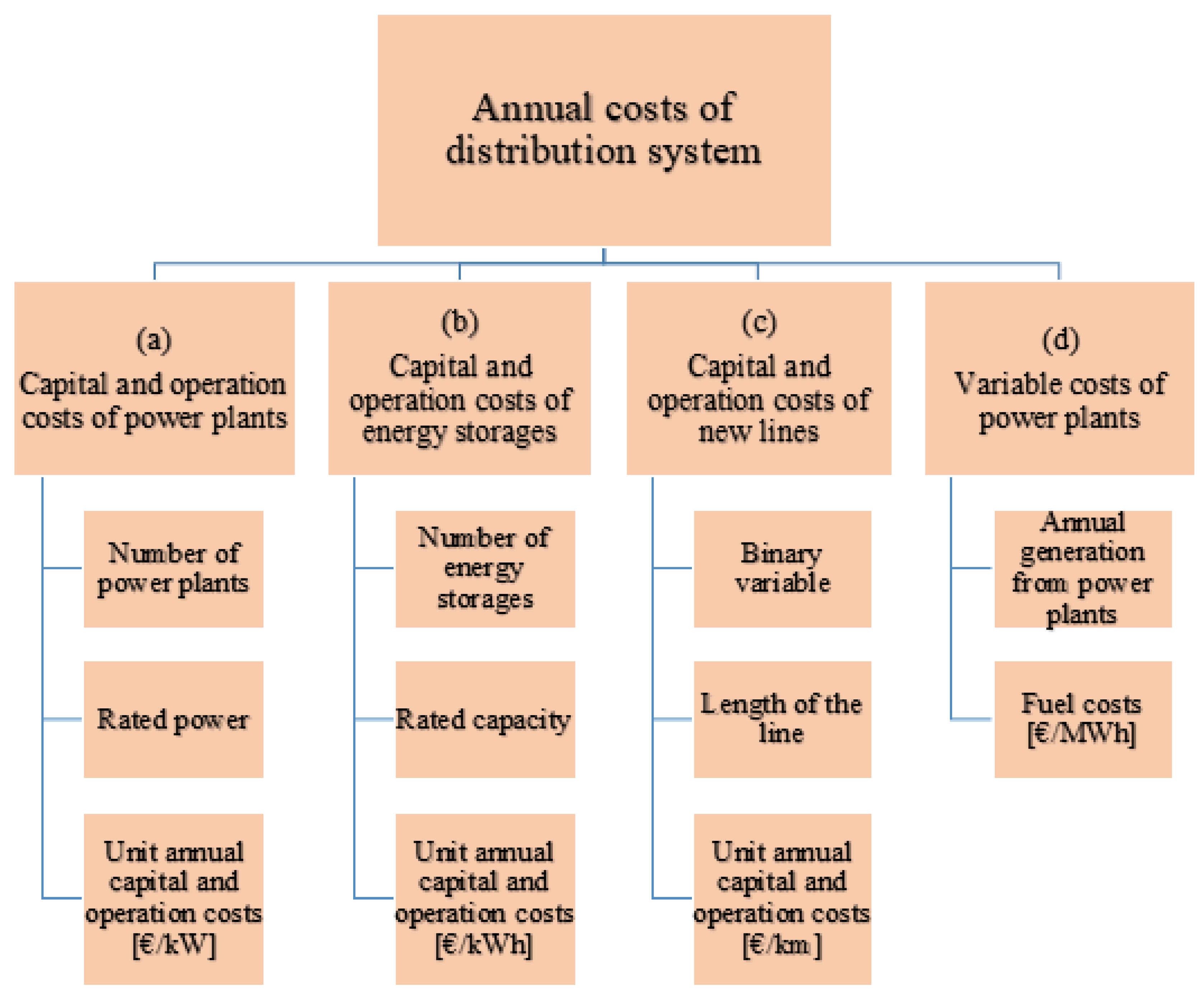
The objective function used in the optimization process consists of the following components expressing costs: capital and a fixed component of operating costs of generating units, capital and a fixed component of operating costs of energy storage, capital and a fixed component of operating costs of permanent new lines in the network, and variable component of operating costs of generating units.
The constraints used in optimization refer to the power and number of units installed in the nodes, the permissible long-term current capacity of the line, the direction of power exchange with the 110 kV system, the level of annual energy production relative to the total demand, power and capacity of energy storage, and voltage level in the nodes.
The optimization time horizon is taken as one year represented by twenty-four representative days.
2.1. Optimization Model
For each node and each renewable energy technology, the generation of electricity is determined on the basis of the number of renewable energy units, the power series, and the utilization of the rated power based on the assumed renewable energy generation profile. However, the demand for electricity in each node depends on the rated power of the installed loads and demand profile.
In each calculation step of the assumed time horizon, power flows in existing lines and new lines are determined, and the amount of power exchange with the transmission system is calculated. Power losses are determined on the basis of power flows, unit resistance, length, and long-term current-carrying capacity of the line. Due to the use of the Mixed-Integer Linear Programming (MILP) model, the losses are linearized.
The difference between the total annual electricity generation from all RES units and the total annual losses in lines is treated as RES energy consumed locally. The level of this consumption is determined before the optimization process as a percentage of the total annual electricity consumption of all loads. In the Appendix A presents a graphical diagram and a table allowing a better understanding of the problem.
2.2. Objective Function
The objective function used in the optimization process is expressed as the sum of the annual costs of the distribution system, including annual fixed costs of generating units, annual fixed costs of energy storage, annual fixed costs of new lines in the network, and operational variable costs.
Fixed costs of generating units are determined on the basis of the number of RES units (), a given capacity series (. ), and unit fixed costs (). The number of renewable energy units is expressed as an integer variable specified for each network node (n), RES technology (d), and values from the power series (r) and stored in a matrix with the dimensions “n” × “d” × “r”. The power series defines the rated power of a single RES generating unit, which is specified for each technology (d) separately. Unit fixed renewable energy costs (capital costs converted into one year and fixed operating costs) are expressed as the average annual investment cost increased by the annual fixed operating costs, determined individually (per kW of installed capacity) for each technology and RES series.
Fixed costs of energy storage units are calculated analogous to the fixed costs of generating units, and their values are determined on the basis of the number of energy storage units in the node (), their nominal capacity (), and unit fixed costs () (designated for 1 kWh of installed energy storage capacity). The number of energy storage units in a node is declared as an integer variable.
Fixed costs of new lines in the network were expressed using a binary variable, determining whether a new line will arise () specified for network nodes (n, w), length of this line () in kilometers, and unit investment costs of one kilometer of a line () specified for each type of line (s).
where:
It was assumed that for the entire time step (one hour), the generated power/load is constant, so the energy for a given time step is determined as the product of power and time (one hour (t′)).
The generation of electricity of a generating unit depends on the sum of the power installed for a given technology “d” in the node “n”, the factor of the utilization of the rated power, and the restrictions imposed on the size of the generation. The use of rated power is impressed as the degree of its use defined for each moment from the adopted time horizon. Generation curtailment is expressed as the power level by which the generation resulting from the power utilization profile is reduced. The total generation in the node can be reduced or increased by the power transmitted to and from the energy storage.
where: —number of units in node n for RES type d and rated power r; —rated power of RES technology d for the power unit series type r; —fixed cost of each type and rated power of renewable energy sources; —number of units in node n for energy storages; —nominal capacity of single energy storage; —fixed cost of energy storages; —binary variable that determines whether a given “s” line will arise between the “n” and “w” nodes; —distance between nodes “n” and “w”; —fixed cost of new lines; —annual energy production from each type of RES r in each node n; —variable cost of each type d and rated power r of renewable energy sources; —total energy from RES type d in node n in time step t; —total production from RES type d in node n in time t; —generation profile for RES technology d in time t; —generation curtailment of RES type d in node n in time t, —total production from RES in node n in time t; . —power which flows from grid to energy storage in node n in time t; —power which flows from energy storage to grid in node n in time t; t′—one hour.
2.3. Constraints
The technical limitations used in the model refer to the level of energy generation, power flows, power losses, a voltage in nodes, and energy storage operation.
The model assumes that annual energy production minus total energy losses in lines must be equal to or greater than its assumed share (k) in the annual demand of all loads in the distribution system under consideration. The annual demand of all loads is expressed as the sum of all the demand in all network nodes in the considered time horizon. The model considers three types of loads (residential, industrial, commercial).
In the analyzed model, only active power flows are considered, assuming that this approach is sufficiently accurate for the purposes of long-term analyses. The power flow in the line between “n” and “w” nodes depends on the generation and demand at these nodes and is expressed as:
The power flow from the 110 kV system to the system under consideration is determined on the basis of the total generation and total demand for the analyzed distribution system.
Power losses in a line are determined as the sum of five linear functions. The value of each function depends on the power flow limitation in the line between “n” and “w” nodes, unit line resistance, the distance between “n” and “w” nodes, power flow, and rated voltage in the analyzed network.
Each linear function was created for different values of power flow in relation to power line capacity. The first function was created for power flow in range 0–100% of line capacity. Rest functions were designed for power flow in ranges: f2: 20–100%, f3: 40–100%, f4: 60–100%, and f5: 80–100% of line capacity. Final power losses were created as a sum of all mentioned linear functions [16]. Equations that describe f1, f2, f3, f4, f5 are presented in Appendix A.
Voltages in nodes are determined on the basis of power flow in the lines and voltages in the nodes that connect these lines, line resistance, and rated voltage of the analyzed system.
The rated capacity of the energy storage at the “n” node is also a limitation on the storage capacity of the storage tanks. It was assumed that the energy storage is described by the efficiency of power exchange with the node, capacity, and power. The tray’s operating cycle is one day when the tray is completely discharged at the beginning and end of the day. The work cycle of the trays has been chosen due to the simplifications resulting from the selection of representative profiles.
where: —annual energy production from each type of RES r in each node; —power losses in a power line between nodes w and k in time t; —consumption of load in node n of type l in time t; —nominal power of load type l in node n; —consumption profile for load type l in time t; —total production from RES type d in node n in time t; —linearized power flow between nodes n and w in time t; —energy exchange between distribution and transmission system in time t; —value of voltage in nodes n/w in time t; —resistance of power line between nodes n and w; —nominal voltage of the distribution system (in this paper, assumed as a 30 kV; —distance between nodes “n” and “w”; —level of charge of energy storages in node n in time t; —number of units in node n for energy storages; —nominal capacity of single energy storage; —efficiency of energy exchange between nodes and energy storages; —power which flows from grid to energy storage in node n in time t; —power which flows from energy storage to grid in node n in time t.
3. Assumptions
It was assumed that it is possible to construct three types of renewable energy technologies: (a) photovoltaic panels, (b) wind turbines, and (c) biogas power plants. Three values of rated power (series) exist that the generating unit may have been selected for each technology (Table 1). Additionally, it was assumed that the total power of all units in one node may not exceed 5 MW except node “1” (node representing 110 kV system), in which no generating source can be installed.
Representative generation profiles have been created for each technology. These profiles were built based on real data for the Polish and German power systems [31,32,33,34,35]. Six profiles have been created for photovoltaic panels and wind turbines, and one profile for biogas power plants, which are constant throughout the considered time horizon, excluding eight days in the summer season, which are intended for renovation and repair. The generation on these days for biogas power plants is zero. Representative profiles for solar panels and wind farms were divided into two types of profiles mapping the high and low generation for three periods of the year: winter, summer, and spring and autumn together.
Representative demand profiles have been created for each type of pickup. These profiles were determined based on data obtained from the Polish DSO [36]. For each type of reception (residential, industrial, commercial), six representative profiles were created for working and non-working days for three periods of the year: winter, summer, and spring and autumn together.
In order to correlate the representative profiles with the actual capacity factor for each technology and the demand profile, it was determined for each period of the year how often a given combination of profiles occurs.
Individual capacity for photovoltaic panels and wind turbines were determined for each node of the analyzed system. This allows you to take into account the differences in sunlight and wind conditions at each node of the network. For biogas power plants, a constant power utilization factor was adopted for all network nodes.
Three types of costs have been determined for each technology and the range of rated power: capital costs, fixed operating costs, and variable costs. All costs are shown in Table 2.
It was assumed that it is possible to allocate one type of energy storage with a capacity of 10 kWh and a power of 5 kW. The efficiency of both energy storage and charging was assumed at 0.9. The energy storage works in a daily cycle, i.e., at the beginning and end of the day, the energy storage has the same state of charge. Capital costs (overnight) and fixed operating costs of the energy reservoir relate to its capacity and amount to € 600/kWh and € 67/kWh, respectively [38].
Two types of lines were also selected that can be used to build new connections between nodes. In Table 3, the types of lines are presented together with their parameters and costs.
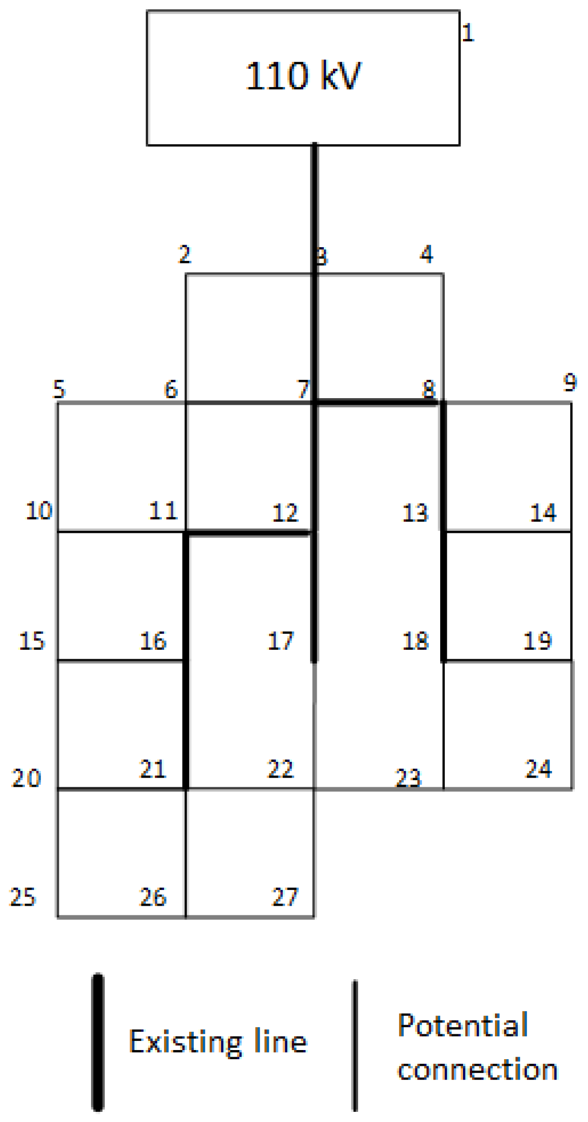
Simulations are carried out using a test network, consisting of 27 nodes, of which node 1 represents a 110 kV system, while nodes 2 to 27 represent a 15 kV system. It was also assumed that the voltage in the nodes must be in the range of 90–110% of the rated voltage (Figure 1).
4. Simulation
Five simulation scenarios with different activities were used for the analysis, which were used to simulate these scenarios (Table 4). These activities include a selection of power and quantity of renewable energy in network nodes, selection of capacity and quantity of energy storage in network nodes, reduction of renewable energy production, and construction of new lines.
The first scenario relates to planning energy clusters in the traditional form, i.e., the selection of generating units. The other scenarios show comprehensive optimization that allows reducing the cost of their operation.
Scenarios
The selection of the power and quantity of RES in network nodes consists of defining the type of generating units, their rated capacities, and their number that should be installed in individual nodes of the network in question. This action is carried out by means of an integer variable (), defining the number of generating units in a given node (n), a given technology (d), and the installed capacity series (r).
The selection of the capacity and number of energy storages in network nodes is based on the selection of the total capacity of energy storage in individual network nodes. This selection is made with the use of an integer variable () that defines the number of energy storage in a given node (n) of the network.
Curtailment of RES generation consists of reducing energy production resulting from representative profiles defined for each of the analyzed technologies. This operation is carried out by means of a real variable (), which determines the generation reduction in a given network node (n), a given technology (d), and at a given time instant (t).
The construction of new lines determines what type of line and between which nodes it will be created. This operation is expressed by a binary variable (), which defines whether a new line of a given type (s) will be created between the network nodes (n, w).
5. Results
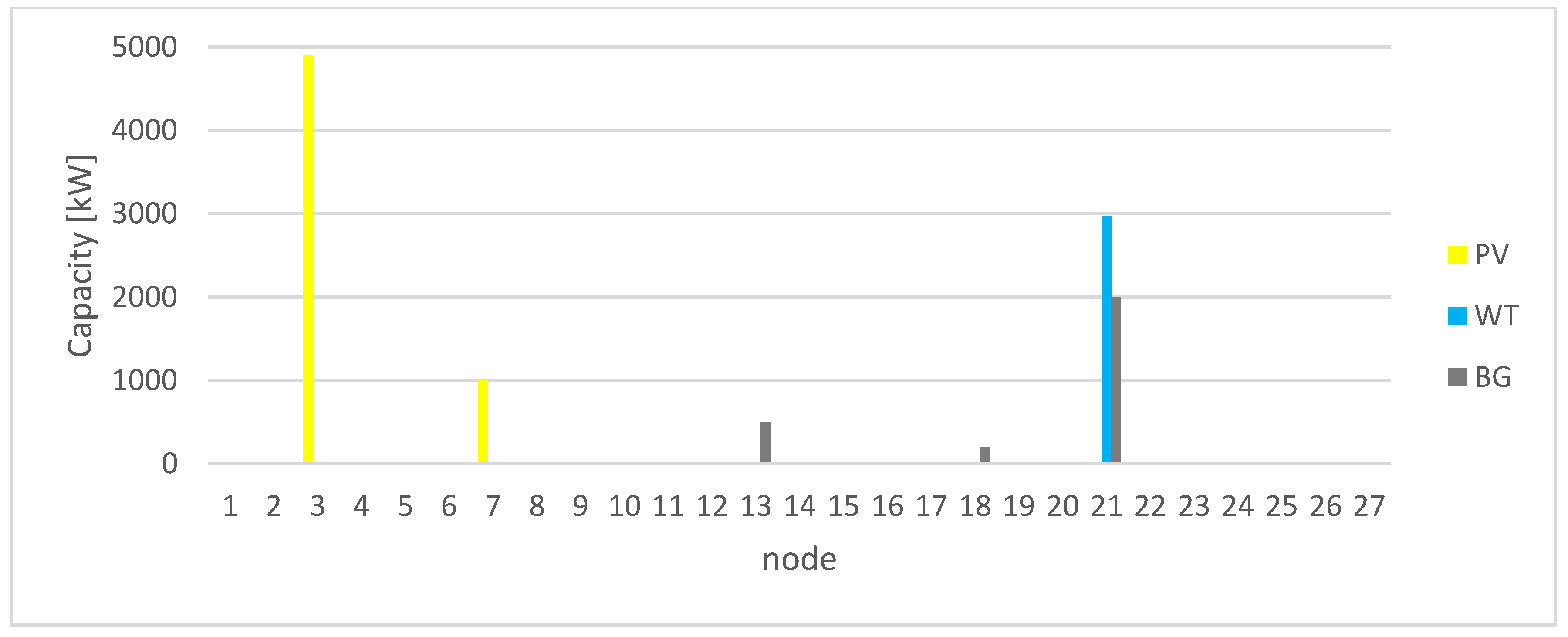
The following section shows the simulation results. The results concern the cost structure and total costs of the development of the distribution system. In the Appendix A, other results are displayed (location of RES, ES, and new lines).
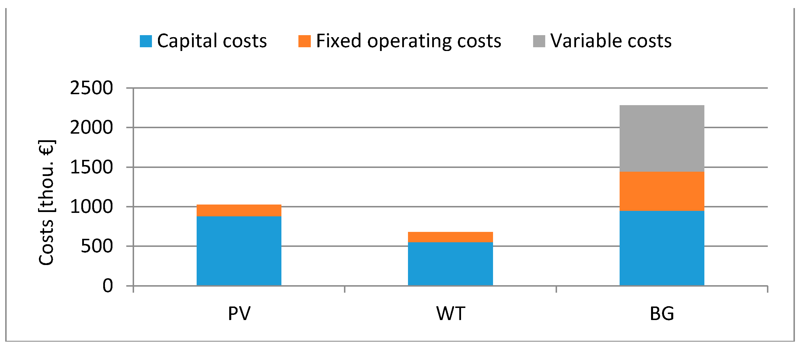
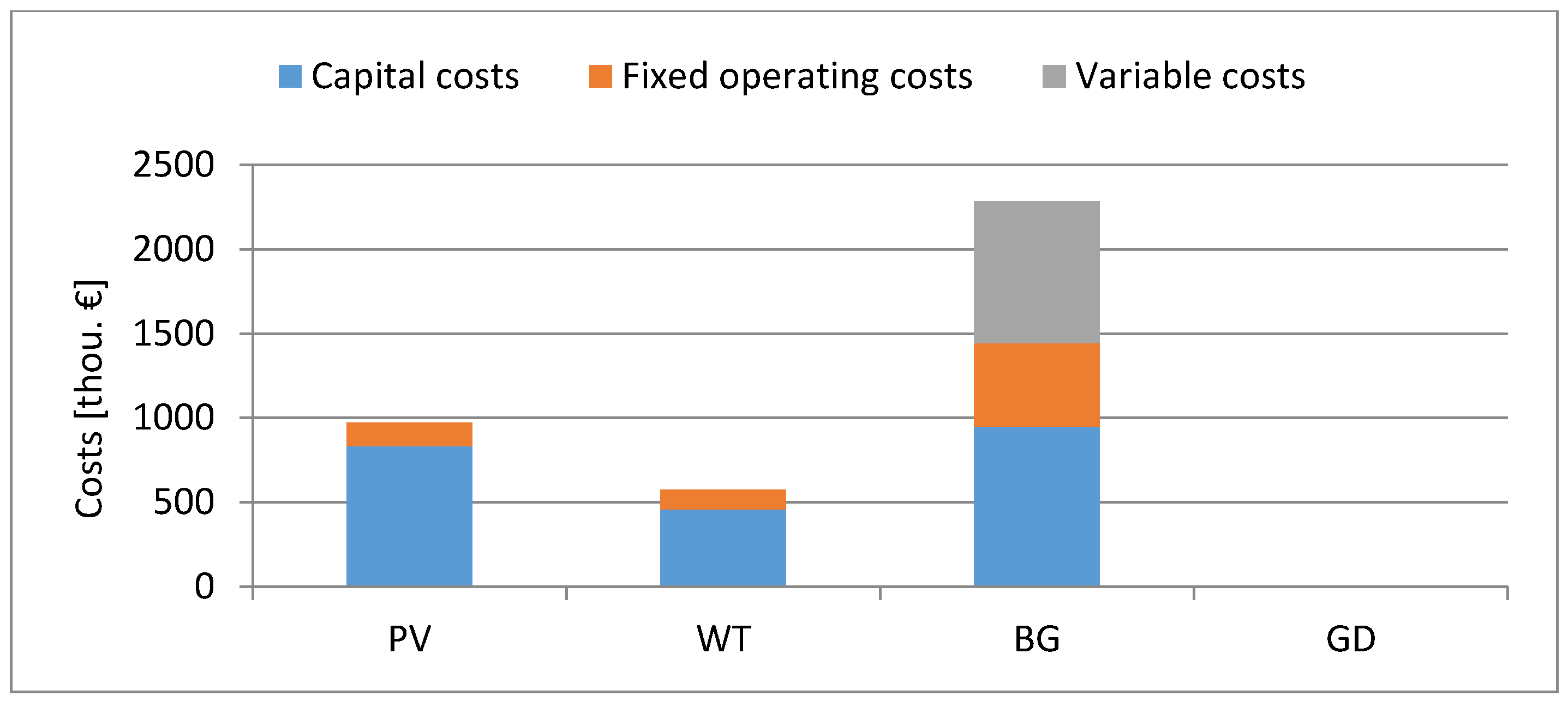
Figure 2 shows the cost structure for scenario “1” for which the largest part of the costs are the costs of biogas plants (approximately 57%). The costs of photovoltaic installations constitute approximately 26%, and wind farms approximately 17%. Moreover, the cost structure for biogas plants is different than in the case of the other two types of generation units. For photovoltaic installations, capital costs are around 86%, and fixed operating costs are 14%; for wind farms, these values are as follows: 80% and 20%. There is one more type of cost for biogas power plants—fixed operating costs (approx. 37%), while fixed capital and operating costs account for 42% and 21%, respectively.
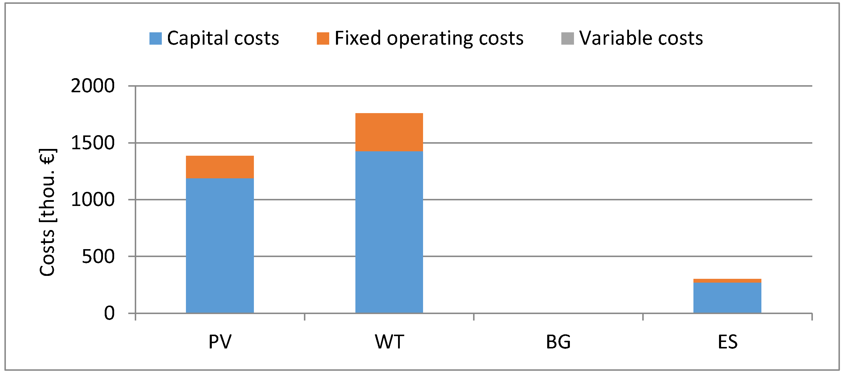
For scenario “2”, the cost structure for photovoltaic installations and wind turbines is similar to those in scenario “1”, for energy storage capital costs constitute 90% of costs and operating costs are fixed at 10%. On the other hand, the structure of total costs is different than in scenario “1” and looks as follows: photovoltaic installations—40%, wind farms—51%, and energy storage—9% (Figure 3).
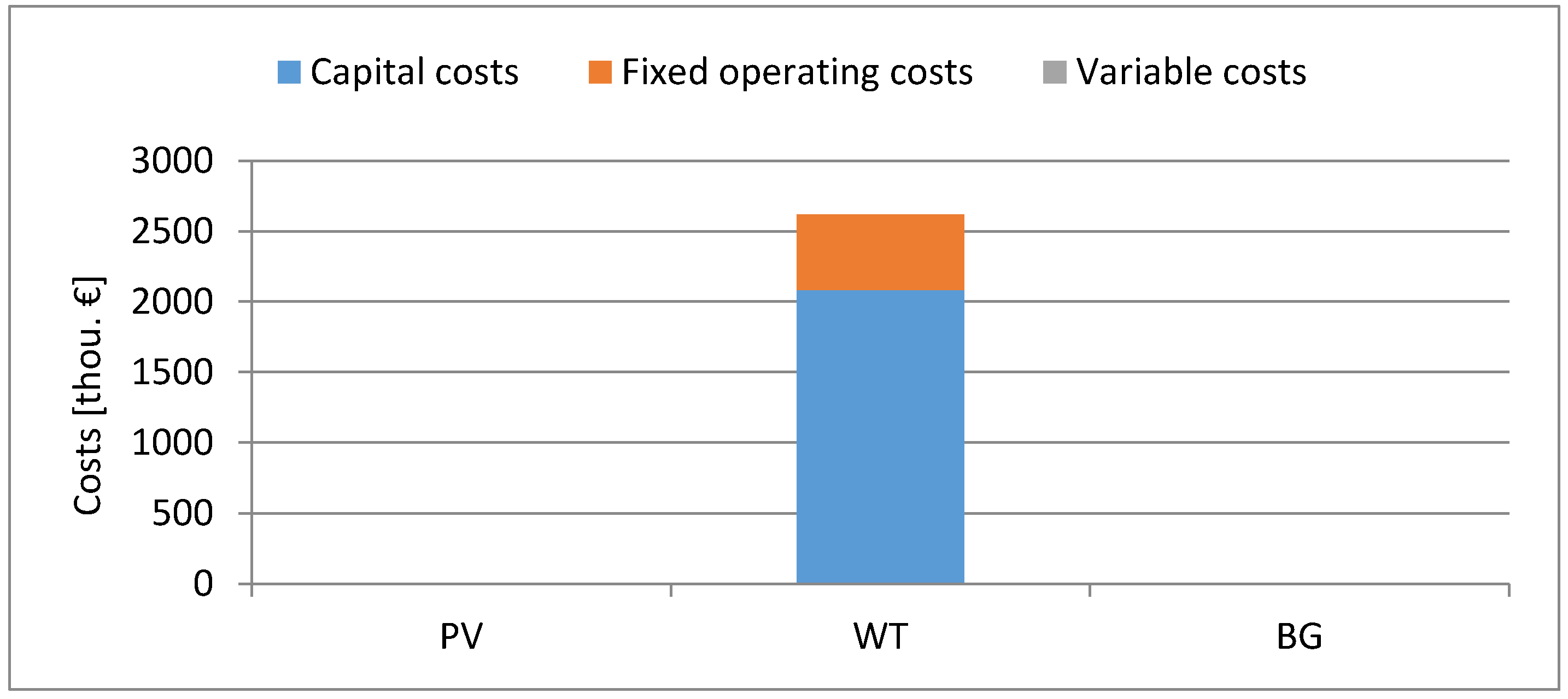
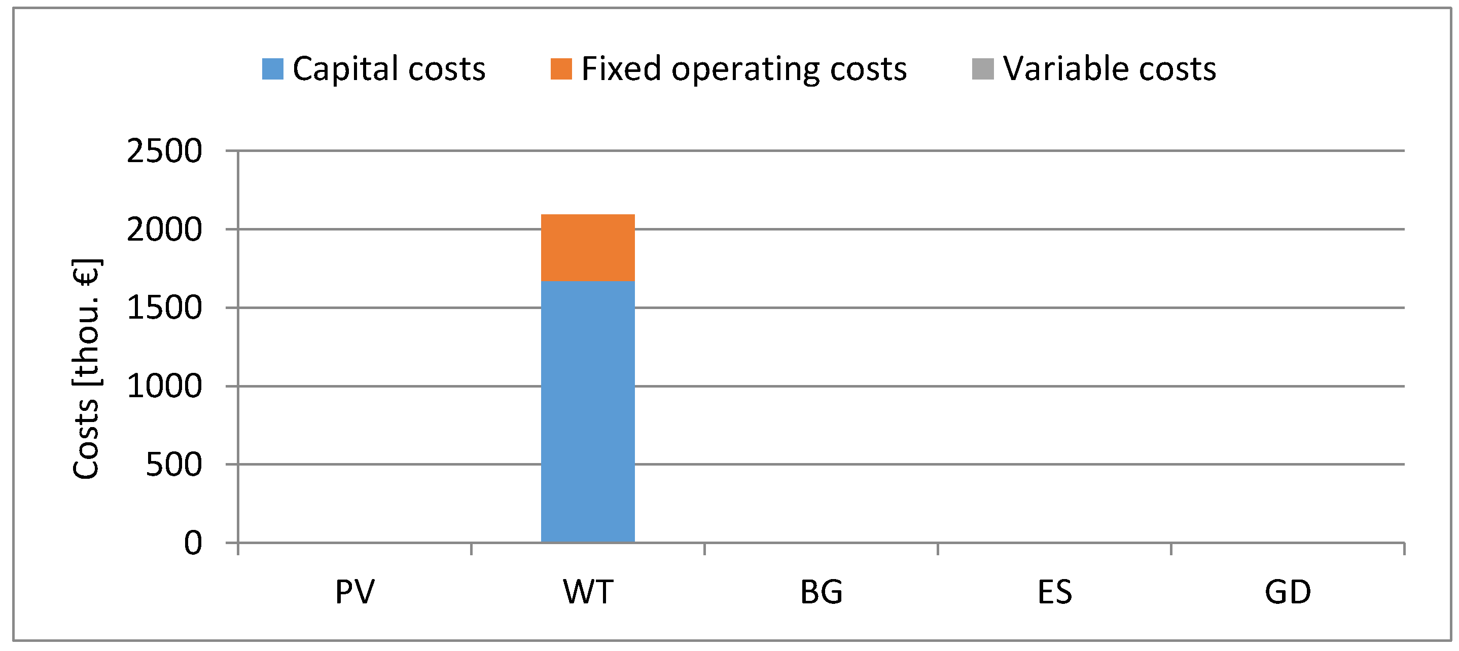
For scenario “3”, for which the selection of power and quantity of RES in the nodes of the analyzed grid and limiting their production was assumed, 100% of the costs are the costs of wind turbines. The capital costs are 85% and the fixed operating costs are 15% of the total costs. These values are different than for the two previous scenarios because only sources with the installed capacity of 500 MW were built, as opposed to the previous scenarios, for which sources with the other types of capacity were also built (Figure 4).
For scenario “4” as for scenario “1”, the largest part of the total costs are the costs of biogas power plants (59%), followed by photovoltaic (PV) installations (25%) and wind turbines (15%). In this scenario, part of the costs is incurred for the construction of new lines (1%) (Figure 5).
Most (99%) of the costs for scenario “5” are the costs of wind turbines and 1% of costs of building new lines. Moreover, each of these costs consists of capital and fixed operating costs in the proportion of, respectively, 80% and 20% for wind turbines and 96% and 4% for the construction of new lines (Figure 6).
The highest costs of development of the analyzed distribution system were obtained for scenario “1”, for which only the selection of power and quantity of RES in nodes was assumed. By adding the selection of capacity and the number of energy storages in the nodes, the overall costs were reduced by 14%. For scenario “3” an additional 21% cost reduction was achieved. The lowest cost reduction in relation to the first scenario was achieved for the 4—4% scenario. However, by assuming all actions together (scenario 5), the lowest system development costs were obtained, which were 48% lower than the costs obtained for scenario “1” (Figure 7).
6. Conclusions
The growing share of renewable energy sources supported by the European Union policy is becoming a challenge for the functioning of power systems. Due to the large expansion of renewable energy sources, whose generation depends on atmospheric conditions (wind farms, PV installations) and the fact that the majority of such installations are connected to distribution systems, this causes increasing problems in the operation of power networks. These problems result from the non-adaptation of distribution systems to the nature of RES work and the age of system components. One of the biggest is the difficulty of planning the operation of systems with a large generation of renewable energy sources (not adapting the generation to demand) and the need for oversize network elements.
One of the solutions to minimize the costs of work planning and the development of distribution systems is comprehensive optimization, taking into account:
- allocation and selection of renewable energy,
- allocation and selection of energy storage capacity,
- reducing renewable energy generation,
- extension of the line
Taking into account the technical aspects of the system operation, capital, and operational costs, each of these activities has specific benefits.
The highest costs of development of the analyzed distribution system were obtained for scenario “1”, for which only the selection of power and quantity of RES in nodes was assumed. Adding the selection of capacity and the number of energy storages in energy-saving nodes cost savings of 14%. For scenario “3”, an additional 21% cost reduction was achieved. The lowest cost reduction of the initial price of the scenarios was obtained for the scenarios “4”—4%. Additionally, after assuming all the works (scenario 5), the minimum development costs were obtained, which were 48% costs of obtaining the scenario “1”.
The allocation and selection of renewable energy capacity allow for better use of existing infrastructure. This operation consists of choosing the type of renewable energy sources, the number of sources from a given power series, and the node in which the units are to be built. Taking into account the generation profiles of individual RES, coefficients of power utilization of these units in individual parts of the network, generation profiles, and capacity of existing lines, it is possible to place such generating units that do not violate the technical parameters of the network and allow achieving the set level of their annual generation at the lowest possible costs total.
The allocation and selection of the capacity of energy storage allow for their distribution in the network and the selection of capacity, which will allow that they will support renewable energy at times when their generation exceeds the total demand in the system. Energy storage allows for energy storage at times when the generation from generating units exceeds the demand (usually these are the night demand valleys) and putting this energy into the network at the peak of demand.
Generation curtailment allows reducing energy production at times when their generation exceeds the total demand, which makes it possible to adjust the generation to the demand in these periods.
The construction of new lines allows the allocation of new units in the nodes, where the coefficient of their power utilization is higher; moreover, this action allows reducing the load on the elements of the existing technical infrastructure of the distribution system.
As the results show, the addition of each of these activities allows you to reduce the costs of operation and development of distribution systems, while the lowest costs are obtained by combining all activities. This shows that the presented mathematical formulation allows for long-term, comprehensive optimization of work planning and development of distribution systems, taking into account the technical aspects of the system, capital, and operational costs.
Funding
This research received no external funding.
Institutional Review Board Statement
Not applicable.
Informed Consent Statement
Not applicable.
Data Availability Statement
Data available in this manuscript.
Acknowledgments
Author would like to express the gratitude to the FICO® corporation for programming support and provision of academic licenses for Xpress Optimization Suite to Lodz University of Technology.
Conflicts of Interest
Author declares no conflict of interest.
Abbreviations
| Sets | |
| n,w ∊ N | sets of indices n,w representing number of nodes in distribution network, |
| d ∊ D | set of indices d representing type of Renewable Energy Sources (RES) technology—D = [d1,…, d3], where d1 is the first possible technology and d3 is the last one, |
| l ∊ L | set of indices l representing number of possible load type. L = [l1,…, l3], where l1 is the first possible type and l3 is the last one, |
| r ∊ R | set of indices r representing type of rated power for each type of possible RES technology, |
| s ∊ S | set of indices s representing type new line which can be built in distribution system |
| Coefficients | |
| annual energy production from each type of RES r in each node n, | |
| total production from RES type d in node n in time t, | |
| total production from RES in node n in time t, | |
| power losses in a power line between nodes w and k in time t, | |
| rated power of RES technology d for the power unit series type r, | |
| total energy from RES type d in node n in time step t, | |
| nominal capacity of single energy storage, | |
| distance between nodes “n” and “w”, | |
| generation profile for RES technology d in time t, | |
| consumption profile for load type l in time t, | |
| nominal power of load type l in node n, | |
| consumption of load in node n of type l in time t, | |
| linearized power flow between nodes n and w in time t, | |
| energy exchange between distribution and transmission system in time t, | |
| resistance of power line between nodes n and w, | |
| nominal voltage of the distribution system (in this paper assumed as a 30 kV), | |
| value of voltage in nodes n/w in time t, | |
| fixed cost of each type and rated power of renewable energy sources, | |
| fixed cost of energy storages, | |
| fixed cost of new lines, | |
| variable cost of each type d and rated power r of renewable energy sources, | |
| level of charge of energy storages in node n in time t, | |
| efficiency of energy exchange between nodes and energy storages, | |
| Decision Variable | |
| number of units in node n for RES type d and rated power r, | |
| number of units in node n for energy storages, | |
| binary variable that determines whether a given “s” line will arise between the “n” and “w” nodes, | |
| generation curtailment of RES type d in node n in time t, | |
| power which flow from grid to energy storage in node n in time t, | |
| power which flow from energy storage to grid in node n in time t, | |
| Acronyms | |
| wind turbine, | |
| photovoltaic installation, | |
| biogas power plant, | |
| renewable energy sources, | |
| ES | energy storages, |
| EC | energy curtailment, |
| GD | grid development. |
Appendix A
Figure A1.
Scheme of the objective function.


Table A1.
Parameters of nodes.
| Fixed Parameters | Variable Parameters |
|---|---|
|
|
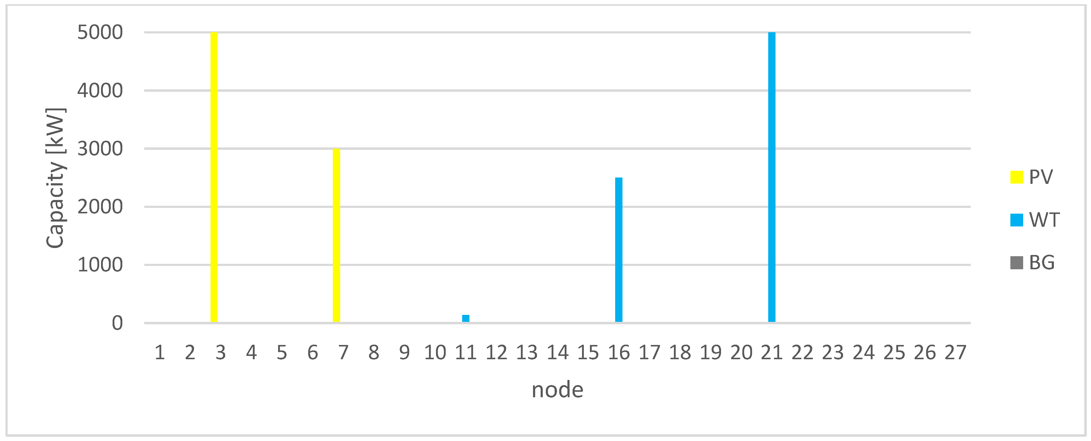
Figure A2.
Capacity structure for scenario “1”.

Figure A3.
Capacity structure for scenario “2”.

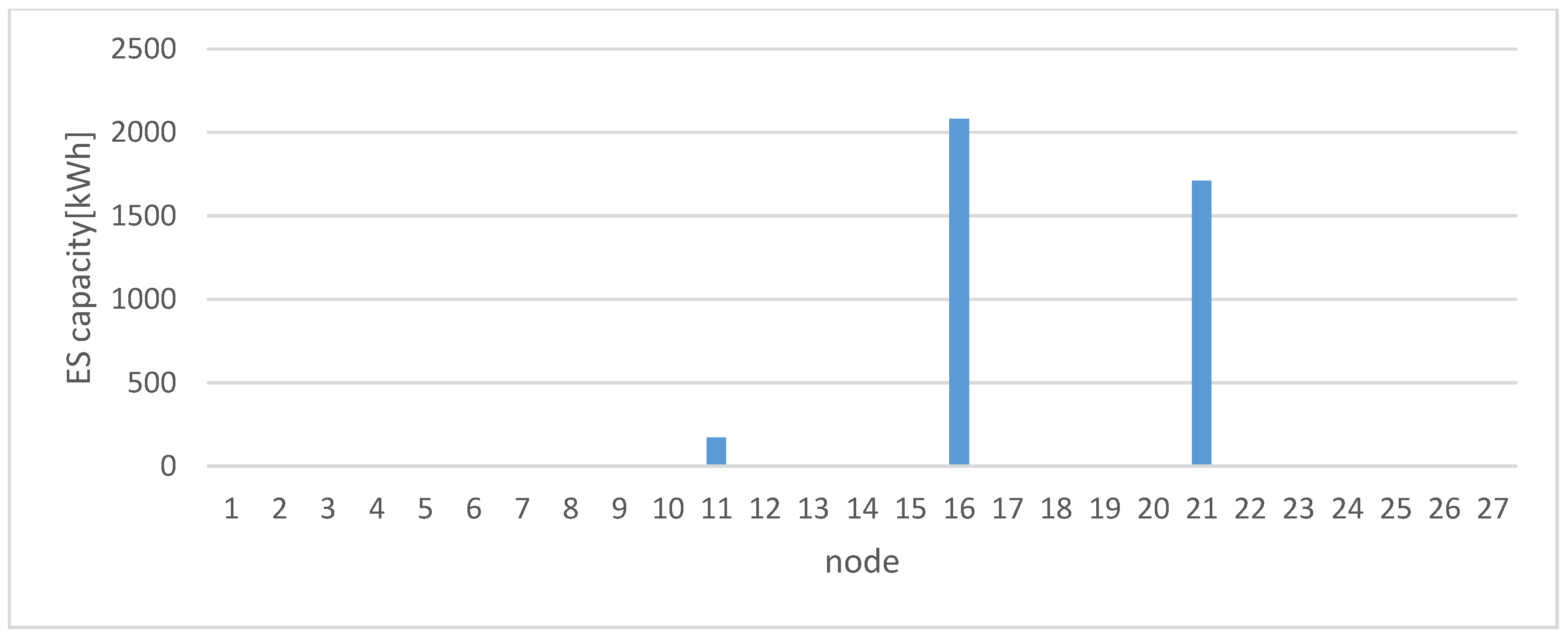
Figure A4.
ES capacity structure for scenario “2”.

Figure A5.
Capacity structure for scenario “3”.

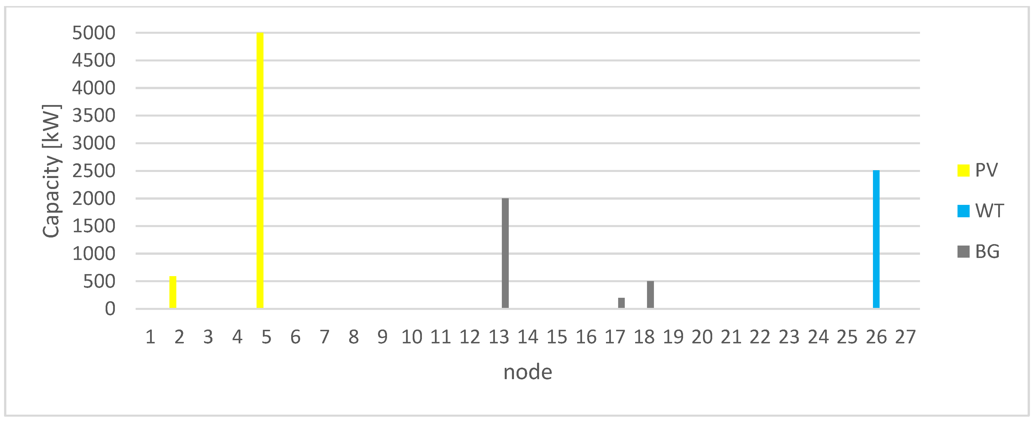
Figure A6.
Capacity structure for scenario “4”.

Figure A7.
Capacity structure for scenario “5”.

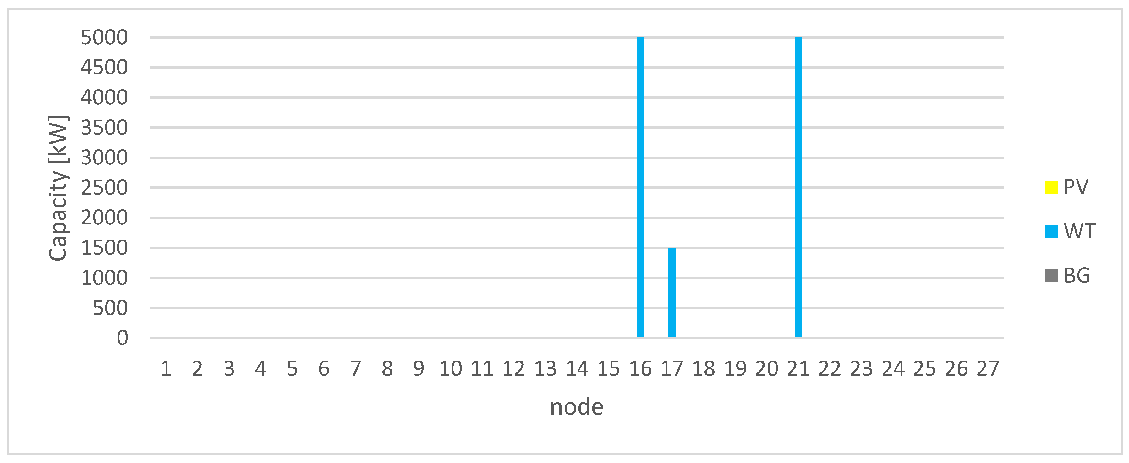
Figure A8.
New lines for scenario “4”.

Figure A9.
New lines for scenario “5”.

Equations corresponding to Equation (9) that describe power losses in lines.
References
- Abu-Mouti, F.; El-Hawary, M. Optimal Distributed Generation Allocation and Sizing in Distribution Systems via Artificial Bee Colony Algorithm. IEEE Trans. Power Deliv. 2011, 26, 2090–2101. [Google Scholar] [CrossRef]
- Prenc, R.; Škrlec, D.; Komen, V. Distributed generation allocation based on average daily load and power production curves. Int. J. Electr. Power Energy Syst. 2013, 53, 612–622. [Google Scholar] [CrossRef]
- Kansal, S.; Sai, B.; Tyagi, B.; Kumar, V. Optimal placement of distributed generation in distribution networks. Int. J. Eng. Sci. Technol. 2011, 3, 47–55. [Google Scholar] [CrossRef]
- Hung, D.Q.; Mithulananthan, N.; Lee, K.Y. Optimal placement of dispatchable and nondispatchable renewable DG units in distribution networks for minimizing energy loss. Int. J. Electr. Power Energy Syst. 2014, 55, 179–186. [Google Scholar] [CrossRef]
- Grisales-Noreña, L.F.; Montoya, D.G.; Ramos-Paja, C.A. Optimal Sizing and Location of Distributed Generators Based on PBIL and PSO Techniques. Energies 2018, 11, 1018. [Google Scholar]
- Keane, A.; O’Malley, M. Optimal utilization of distribution networks for energy harvesting. IEEE Trans. Power Syst. 2007, 22, 467–475. [Google Scholar] [CrossRef]
- Khalesi, N.; Rezaei, N.; Haghifam, M. DG allocation with application of dynamic programming for loss reduction and reliability improvement. Electr. Power Energy Syst. 2011, 33, 288–295. [Google Scholar] [CrossRef]
- Kuri, B.; Redfern, M.; Li, F. Optimization of rating and positioning of dispersed generation with minimum network disruption. IEEE Power Eng. Soc. Gen. Meet. 2004. [Google Scholar] [CrossRef]
- Mashayekh, S.; Stadler, M.; Cardoso, G.; Heleno, M. A mixed integer linear programming approach for optimal DER portfolio, sizing, and placement in multi-energy microgrids. Appl. Energy 2017, 187, 154–168. [Google Scholar] [CrossRef] [Green Version]
- Rueda-Medina, A.; Franco, J.F.; Rider, M.; Padilha-Feltrin, A.; Romero, R. A mixed-integer linear programming approach for optimal type, size and allocation of distributed generation in radial distribution systems. Electr. Power Syst. Res. 2013, 97, 133–143. [Google Scholar] [CrossRef]
- Jamian, J.; Mustafa, M.; Mokhlis, H.; Baharudin, M. Simulation study on optimal placement and sizing of battery switching station units using Artificial Bee Colony algorithm. Electr. Power Energy Syst. 2014, 55, 592–601. [Google Scholar] [CrossRef]
- Zheng, Y.; Dong, Z.; Luo, F. Optimal allocation of energy storage system for risk mitigation of DISCOs with high renewable penetrations. IEEE Trans. Power Syst. 2014, 21, 212–220. [Google Scholar] [CrossRef]
- Carpinelli, G.; Mottola, F. Optimal allocation of dispersed generators, capacitors and distributed energy storage systems in distribution networks. In 2010 Modern Electric Power Systems; IEEE: Piscataway, NJ, USA, 2010; pp. 1–6. [Google Scholar]
- Garcia, R.; Weisser, D. A wind–diesel system with hydrogen storage: Joint optimisation of design and dispatch. Renew. Energy 2006, 31, 2296–2320. [Google Scholar] [CrossRef]
- Gomez-Gonzalez, M.; Hernandez, J.C.; Vera, D.; Jurado, F. Optimal sizing and power schedule in PV household-prosumers for improving PV self-consumption and providing frequency containment reserve. Energy 2019, 191, 116554. [Google Scholar] [CrossRef]
- Andrychowicz, M. Comparison of the Use of Energy Storages and Energy Curtailment as an Addition to the Allocation of Renewable Energy in the Distribution System in Order to Minimize Development Costs. Energies 2020, 13, 3746. [Google Scholar] [CrossRef]
- Heris, M.-N.; Mirzaei, M.A.; Asadi, S.; Mohammadi-Ivatloo, B.; Jebelli, H.; Marzband, M. Evaluation of hydrogen storage technology in risk-constrained stochastic scheduling of multi-carrier energy systems considering power, gas and heating network constraints. Int. J. Hydrog. Energy 2020, 45, 30129–30141. [Google Scholar] [CrossRef]
- Delille, G.; Malarange, G.; Gaudin, C. Analysis of the options to reduce the integration costs of renewable generation in the distribution networks. Part 2: A step towards advanced connection studies taking into account the alternatives to grid reinforcement. In Proceedings of the CIRED, 22nd International Conference on Electricity Distribution, Stockholm, Sweden, 10–13 June 2013. [Google Scholar]
- Pagnetti, A.; Fournel, J.; Santander, C.; Minaud, A. A comparison of different curtailment strategies for distributed generation. In Proceedings of the CIRED, 23rd International Conference on Electricity Distribution, Lyon, France, 15–18 June 2015. [Google Scholar]
- Tonkoski, R.; Lopes, L.; El-Fouly, T.H. Coordinated Active Power Curtailment of Grid Connected PV Inverters for Overvoltage Prevention. IEEE Trans. Sustain. Energy 2011, 2, 139–147. [Google Scholar] [CrossRef]
- Sun, W.; Harrison, G.P. Influence of generator curtailment priority on network hosting capacity. In Proceedings of the CIRED, 22nd International Conference on Electricity Distribution, Stockholm, Sweden, 10–13 June 2013. [Google Scholar]
- Freitas, P.F.S.; Macedo, L.H.; Romero, R. A strategy for transmission network expansion planning considering multiple generation scenarios. Electr. Power Syst. Res. 2019, 172, 22–31. [Google Scholar] [CrossRef]
- Paiva, P.; Khodr, H.; Domínguez-Navarro, J.; Yusta, J.; Urdaneta, A. Integral planning of primary–secondary distribution systems using mixed integerlinear programming. IEEE Trans. Power Syst. 2005, 20, 1134–1143. [Google Scholar] [CrossRef]
- Türkay, B.; Artac, T. Optimal distribution network design using genetic algorithms. Electr. Power Compon. Syst. 2005, 33, 513–524. [Google Scholar] [CrossRef]
- Martins, V.; Borges, C. Active distribution network integrated planningincorporating distributed generation and load response uncertainties. IEEE Trans. Power Syst. 2011, 26, 2164–2172. [Google Scholar] [CrossRef]
- Haffner, S.; Pereira, L.; Pereira, L.; Barreto, L. Multistage model for dis-tribution expansion planning with distributed generation—Part I: Problemformulation. IEEE Trans. Power Deliv. 2008, 23, 915–923. [Google Scholar] [CrossRef]
- Haffner, S.; Pereira, L.; Pereira, L.; Barreto, L. Multistage model for dis-tribution expansion planning with distributed generation—Part II: Numericalresults. IEEE Trans. Power Deliv. 2008, 23, 924–929. [Google Scholar] [CrossRef]
- Celli, G.; Mocci, S.; Pilo, F.; Bertini, D.; Cicoria, R.; Corti, S. Multi-year optimal planning of active distribution networks. In Proceedings of the CIRED, 22th International Conference on Electricity Distribution, Vienna, Italy, 21–24 May 2007. [Google Scholar]
- Canizes, B.; Soaresa, J.; Lezamaa, F.; Silvaa, C.; Valea, Z.; Corchadobcd, J.M. Optimal expansion planning considering storage investment and seasonal effect of demand and renewable generation. Renew. Energy 2019, 138, 937–954. [Google Scholar] [CrossRef]
- Dargahi, A.; Sanjani, K.; Nazari-Heris, M.; Mohammadi-Ivatloo, B.; Tohidi, S.; Marzband, M. Scheduling of Air Conditioning and Thermal Energy Storage Systems Considering Demand Response Programs. Sustainability 2020, 12, 7311. [Google Scholar] [CrossRef]
- Pse, S.A.; Polish, T.S.O. Available online: https://www.pse.pl/dane-systemowe (accessed on 7 January 2020).
- 50HZ; Genrma, T.S.O. Available online: https://www.50hertz.com (accessed on 7 January 2020).
- Amprion; Genrman, T.S.O. 2015. Available online: https://www.amprion.net/ (accessed on 7 January 2020).
- Teene, T.; Genrman, T.S.O. Available online: http://www.tennet.eu/ (accessed on 7 January 2020).
- Transnet, B.W.; Genrman, T.S.O. 2015. Available online: https://www.transnetbw.com (accessed on 7 January 2020).
- Pge Dystrybucja, S.A.; Polish, D.S.O. Available online: https://pgedystrybucja.pl/content/download/2038/file/iriesd_pge-dystrybucja-sa_tekst-jednolity_od_27_08_2020.pdf (accessed on 7 January 2020).
- Impact Assesment-Ocena Skutków Regulacji do Projektu Ustawy o Odnawialnych Źródłach Energii, 12 November 2013. Available online: http://www.toe.pl/pl/wybrane-dokumenty/rok-2013?download=72:ocena-skutkow-regulacji (accessed on 7 January 2020).
- Lazard. Lazard’s Levelized Cost of Storage Analysis. November 2018. Available online: https://www.lazard.com/media/450774/lazards-levelized-cost-of-storage-version-40-vfinal.pdf (accessed on 7 January 2020).
Figure 1.
Benchmark model of medium voltage distribution network [16].
Figure 1.
Benchmark model of medium voltage distribution network [16].

Figure 2.
The cost structure for scenario “1”.

Figure 3.
The cost structure for scenario “2”.

Figure 4.
The cost structure for scenario “3”.

Figure 5.
The cost structure for scenario “4”.

Figure 6.
The cost structure for scenario “5”.

Figure 7.
Total costs of the development of the distribution system.

Table 1.
Rated power of Renewable Energy Sources (RES).
| Technology | Capacity [kW] | ||
|---|---|---|---|
| Photovoltaic panels | 10 | 100 | 1000 |
| Wind turbines | 10 | 100 | 500 |
| Biogas power plants | 200 | 500 | 2000 |
Table 2.
RES costs [37].
Table 2.
RES costs [37].
| Technology | PV | WT | BG | ||||||
|---|---|---|---|---|---|---|---|---|---|
| Rated power [kW] | 10 | 100 | 1000 | 10 | 100 | 500 | 200 | 500 | 2000 |
| Capital costs [mln €/MW] | 1.3 | 1.3 | 1.2 | 1.7 | 1.7 | 1.5 | 3.3 | 3 | 2.9 |
| Fixed operating costs [thou. €/MW/annum] | 27.4 | 27.4 | 24.3 | 34.1 | 34.1 | 46.2 | 197.6 | 187.4 | 185.5 |
| Variable costs [€/MWh] | 0 | 0 | 0 | 0 | 0 | 0 | 93.6 | 80 | 71.7 |
Table 3.
Parameters of new lines.
| Line Cross Section [mm2] | Computational Resistance [Ω/km] | Long-Term Current Carrying Capacity [A] | Capital Costs [€/km] | Fixed Operating Costs [€/km] |
|---|---|---|---|---|
| 50 | 0.59 | 228 | 51,667 | 60,000 |
| 70 | 0.43 | 280 | 2071 | 2405 |
Table 4.
Assumed scenarios.
| Scenario | Activities |
|---|---|
| 1 |
|
| 2 |
|
| 3 |
|
| 4 |
|
| 5 |
|
Publisher’s Note: MDPI stays neutral with regard to jurisdictional claims in published maps and institutional affiliations. |
© 2021 by the author. Licensee MDPI, Basel, Switzerland. This article is an open access article distributed under the terms and conditions of the Creative Commons Attribution (CC BY) license (http://creativecommons.org/licenses/by/4.0/).
Share and Cite
MDPI and ACS Style
Andrychowicz, M. RES and ES Integration in Combination with Distribution Grid Development Using MILP. Energies 2021, 14, 383. https://0-doi-org.brum.beds.ac.uk/10.3390/en14020383
AMA Style
Andrychowicz M. RES and ES Integration in Combination with Distribution Grid Development Using MILP. Energies. 2021; 14(2):383. https://0-doi-org.brum.beds.ac.uk/10.3390/en14020383
Chicago/Turabian StyleAndrychowicz, Mateusz. 2021. "RES and ES Integration in Combination with Distribution Grid Development Using MILP" Energies 14, no. 2: 383. https://0-doi-org.brum.beds.ac.uk/10.3390/en14020383
Note that from the first issue of 2016, this journal uses article numbers instead of page numbers. See further details here.