A New MPPT Algorithm for Photovoltaic Power Generation under Uniform and Partial Shading Conditions

 ,
,
Abstract
:
1. Introduction
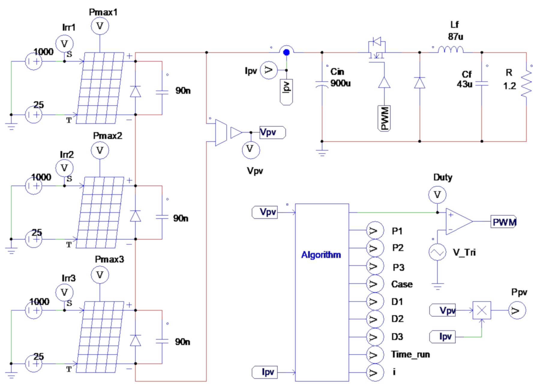
2. PV and Buck Converter Modeling
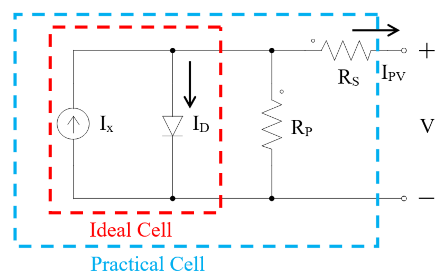
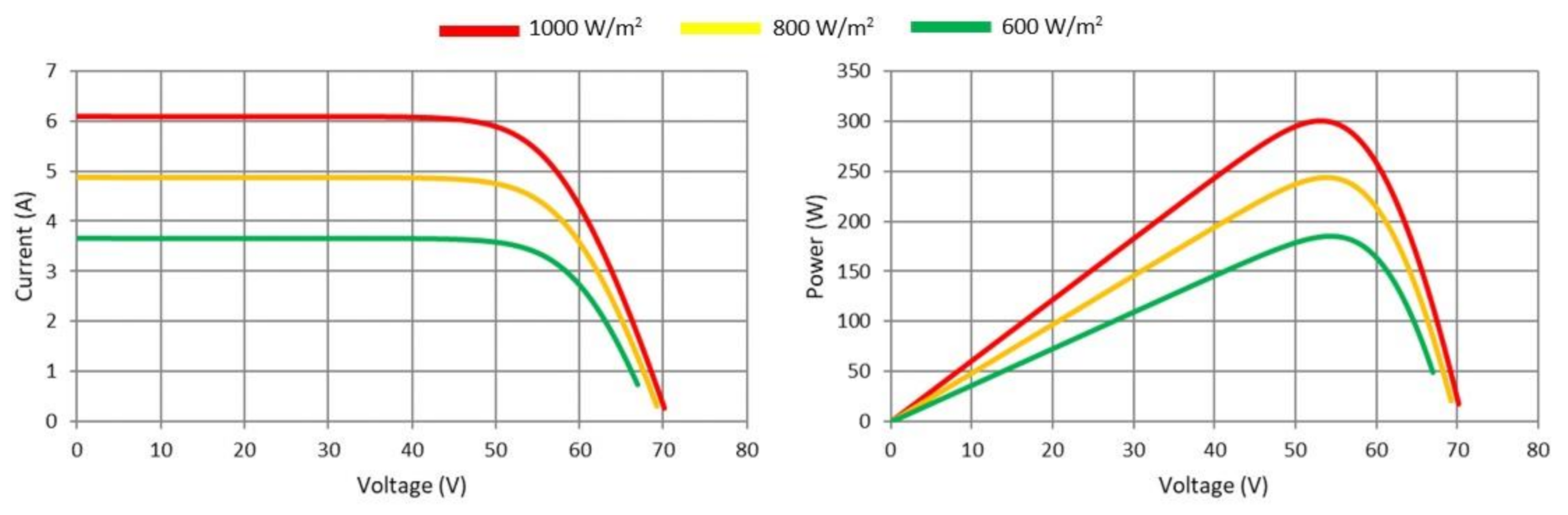
2.1. PV Cell Modeling
2.2. Partial Shading and Its Effects
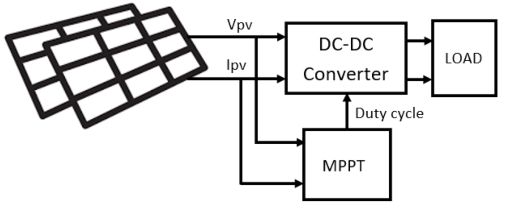
2.3. Buck Converter
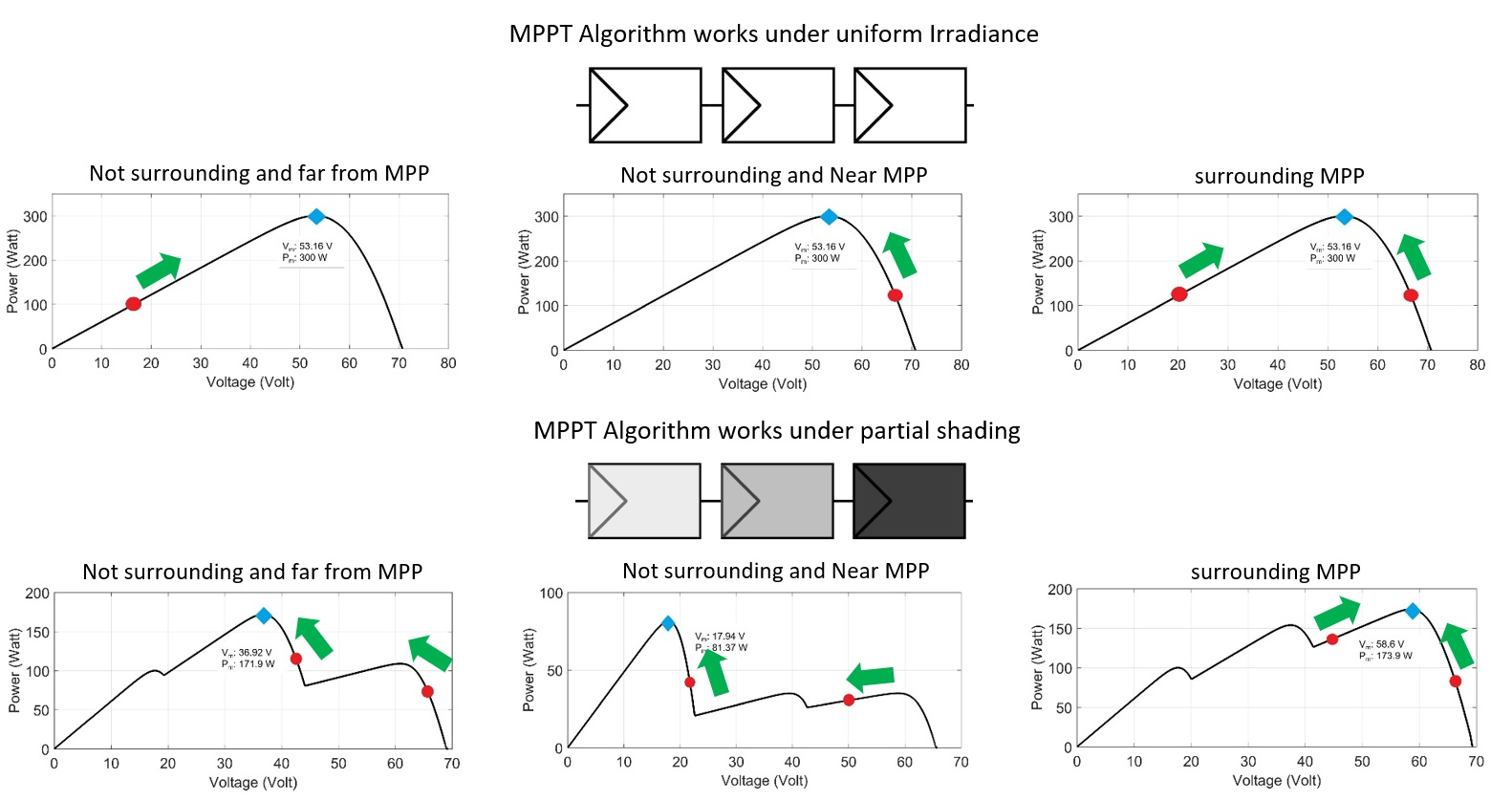
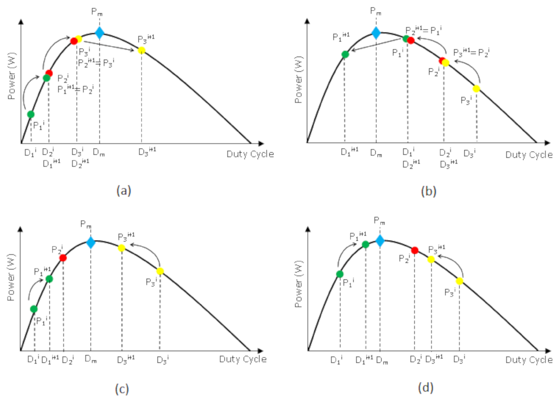
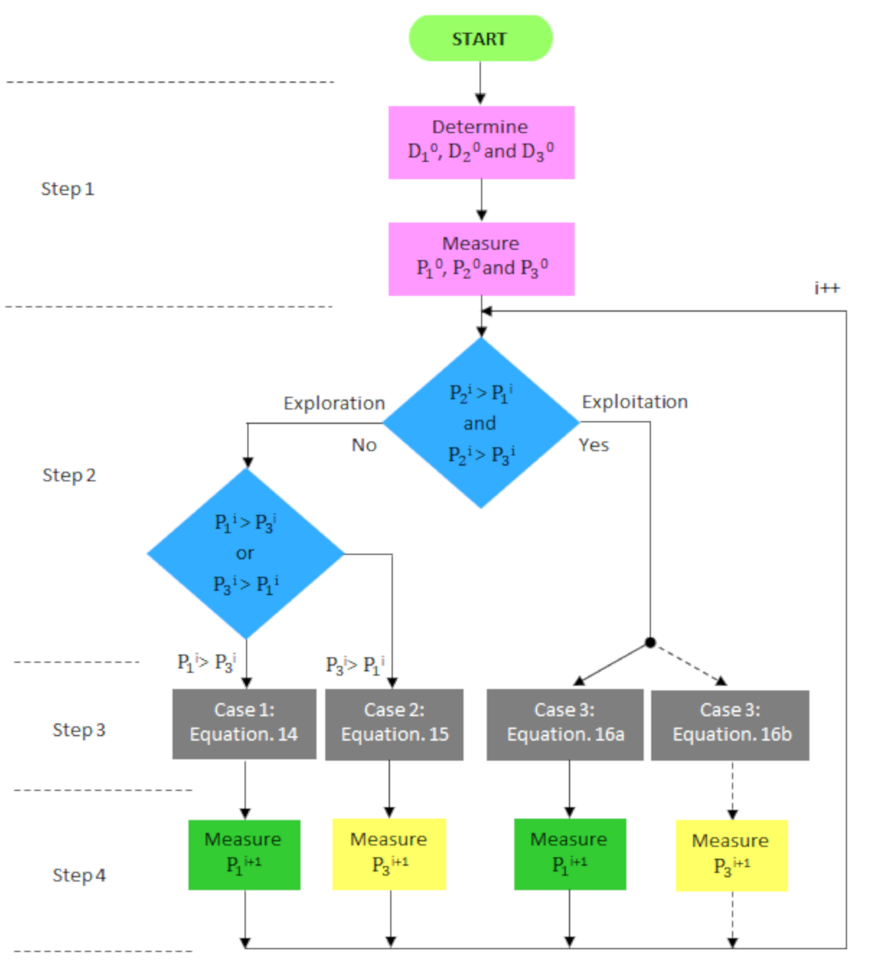
3. Proposed Algorithm
D2i+1 = D1i; D3i+1 = D2i
P2i+1 = P1i; P3i+1 = P2i
D1i+1 = D2i; D2i+1 = D3i
P1i+1 = P2i; P2i+1 = P3i
4. Simulations and Results
- (a)
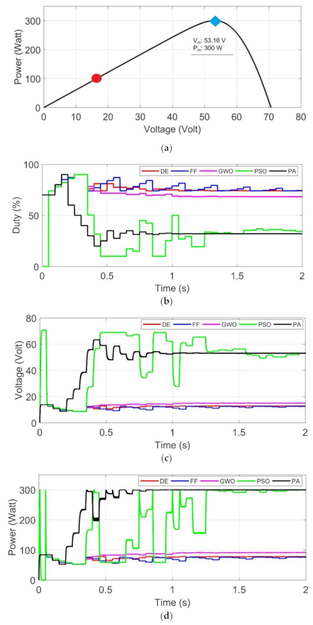
- DE, FF, PSO and GWO algorithms are implemented using five particles, while the proposed algorithm is using three particles to simplify the coding implementation.
- (b)
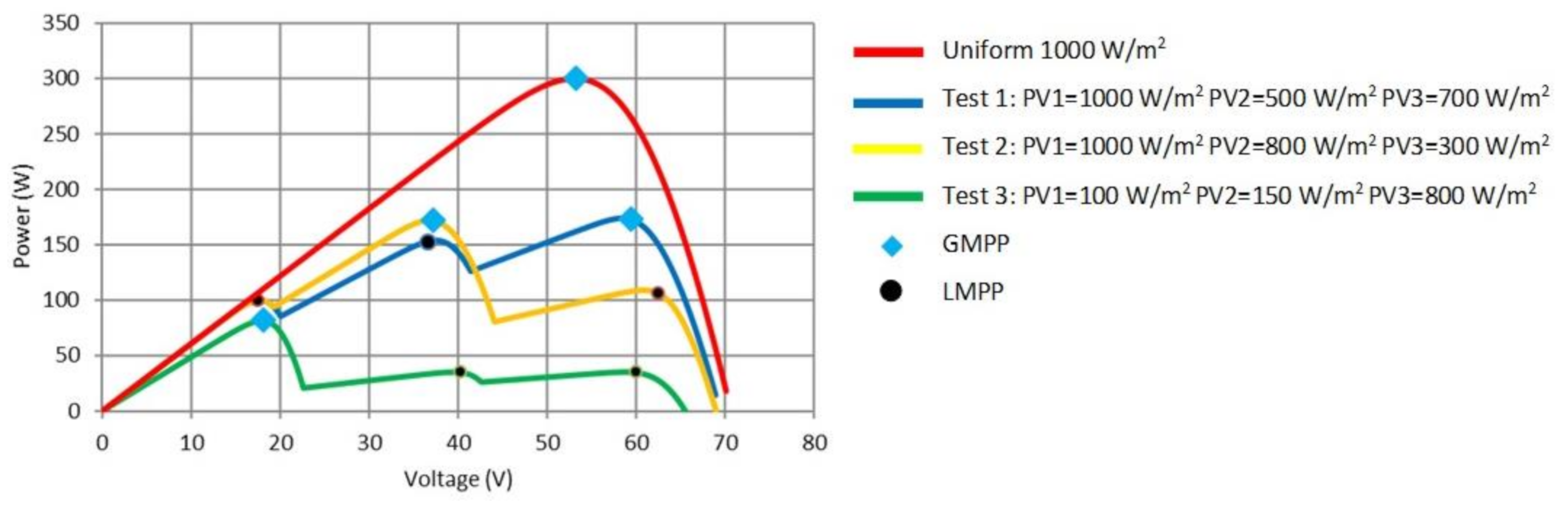
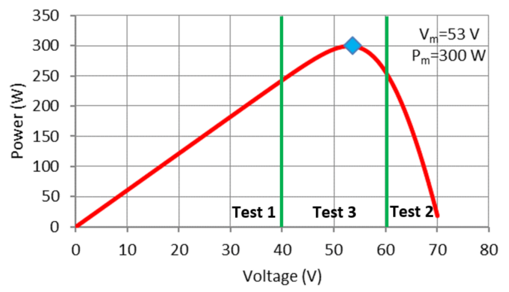
- Uniform irradiance tests: constant irradiance at STC (1000 W/m2 and 25 °C), targeted MPP is (Test 1) far from initial positions of particles, (Test 2) near initial positions, and (Test 3) laid between initial positions.
- (c)
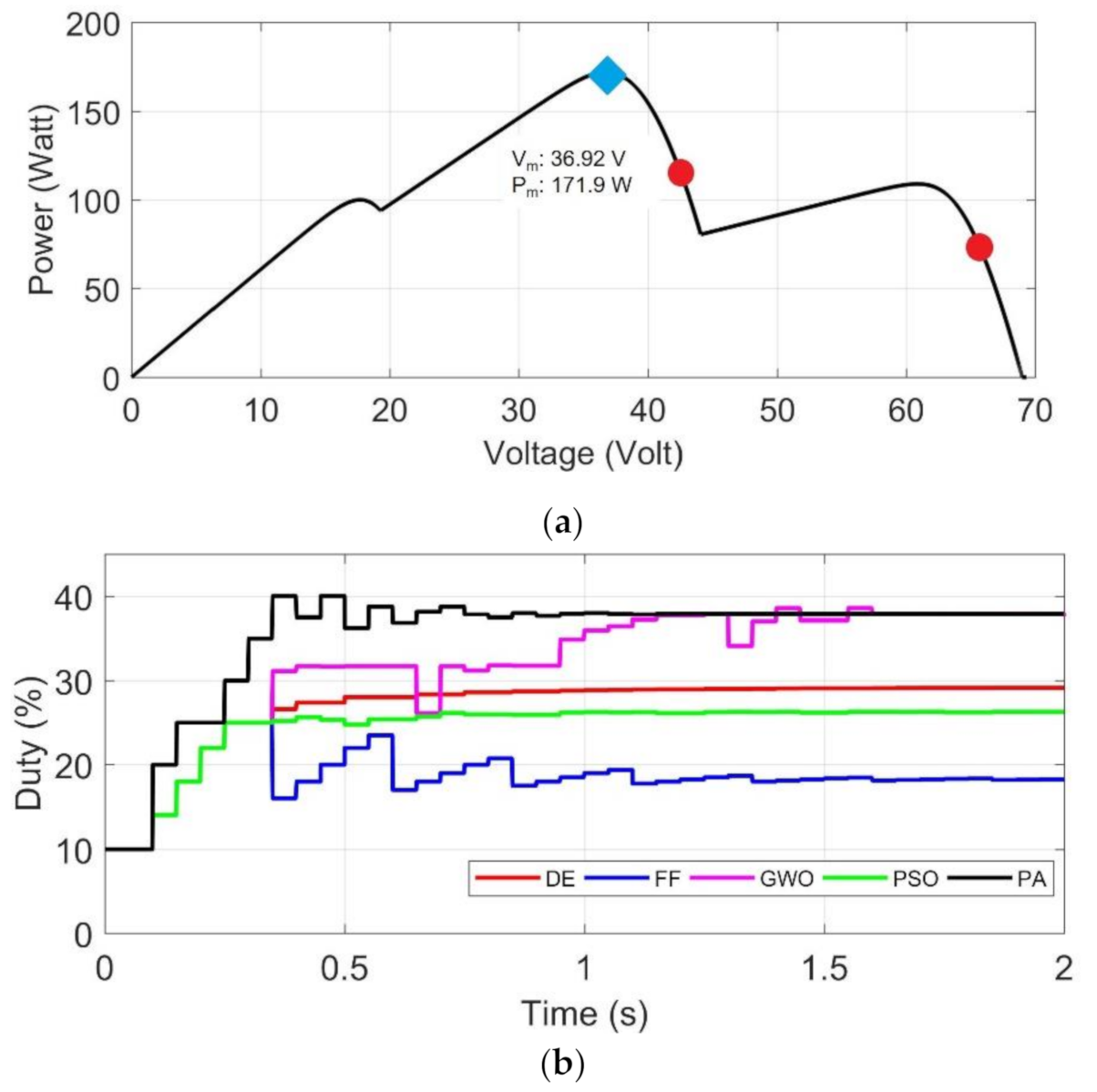
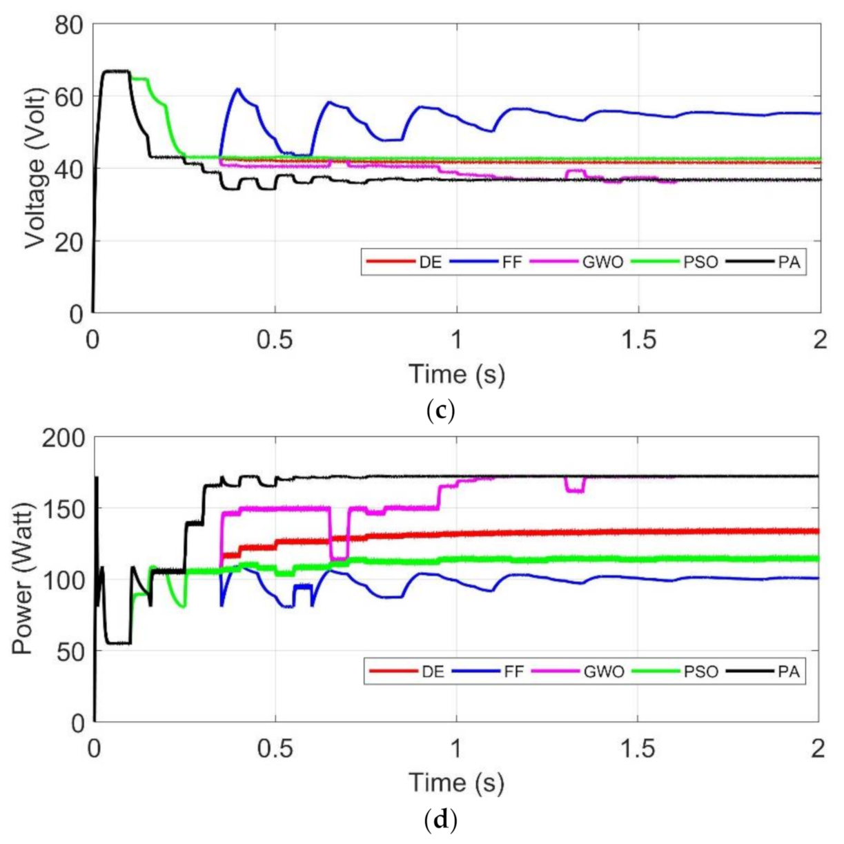
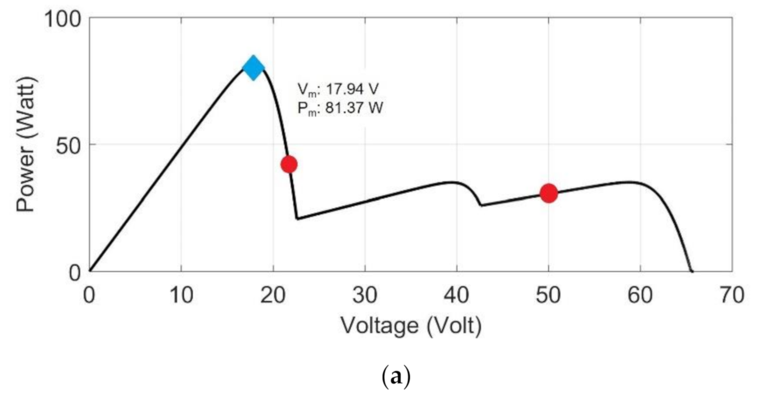
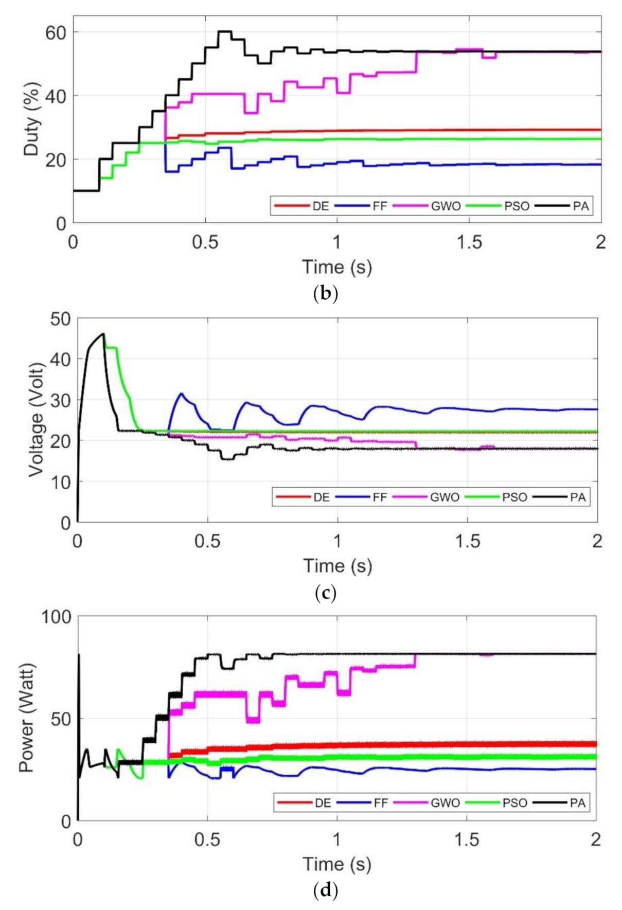
- Partial shading tests: targeted GMPP is (Test 4) laid between initial particles, (Test 5) near initial particles, and (Test 6) far from the initial particles with similar value of power points.
- (d)
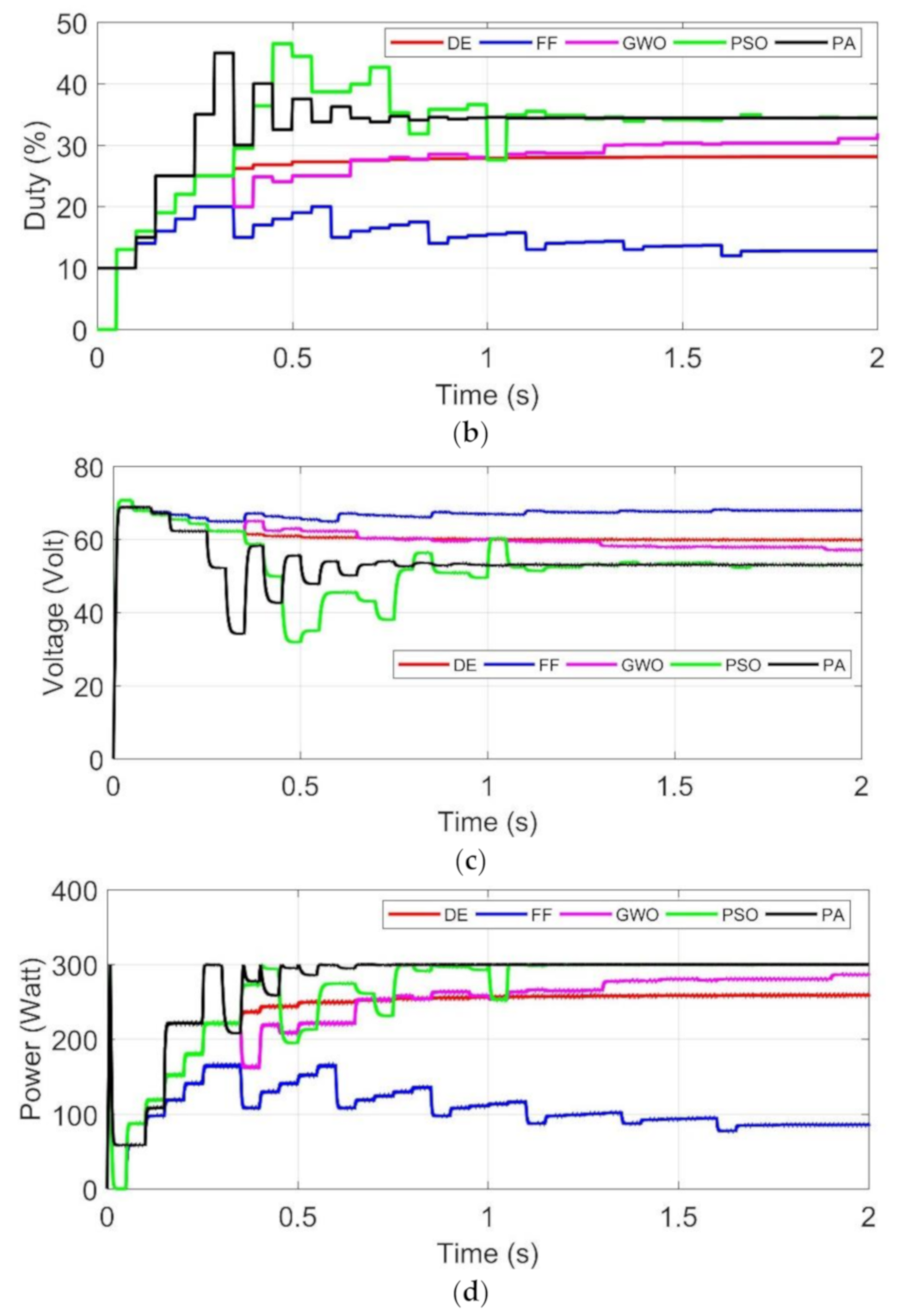
- To verify the performance, each algorithm is tested 10 times for each test 1–6. Duration of energy harvesting process in simulation is 2 s. Sample test is provided in Section 4.1. Uniform Irradiance test and 4.2. Partial Shading.
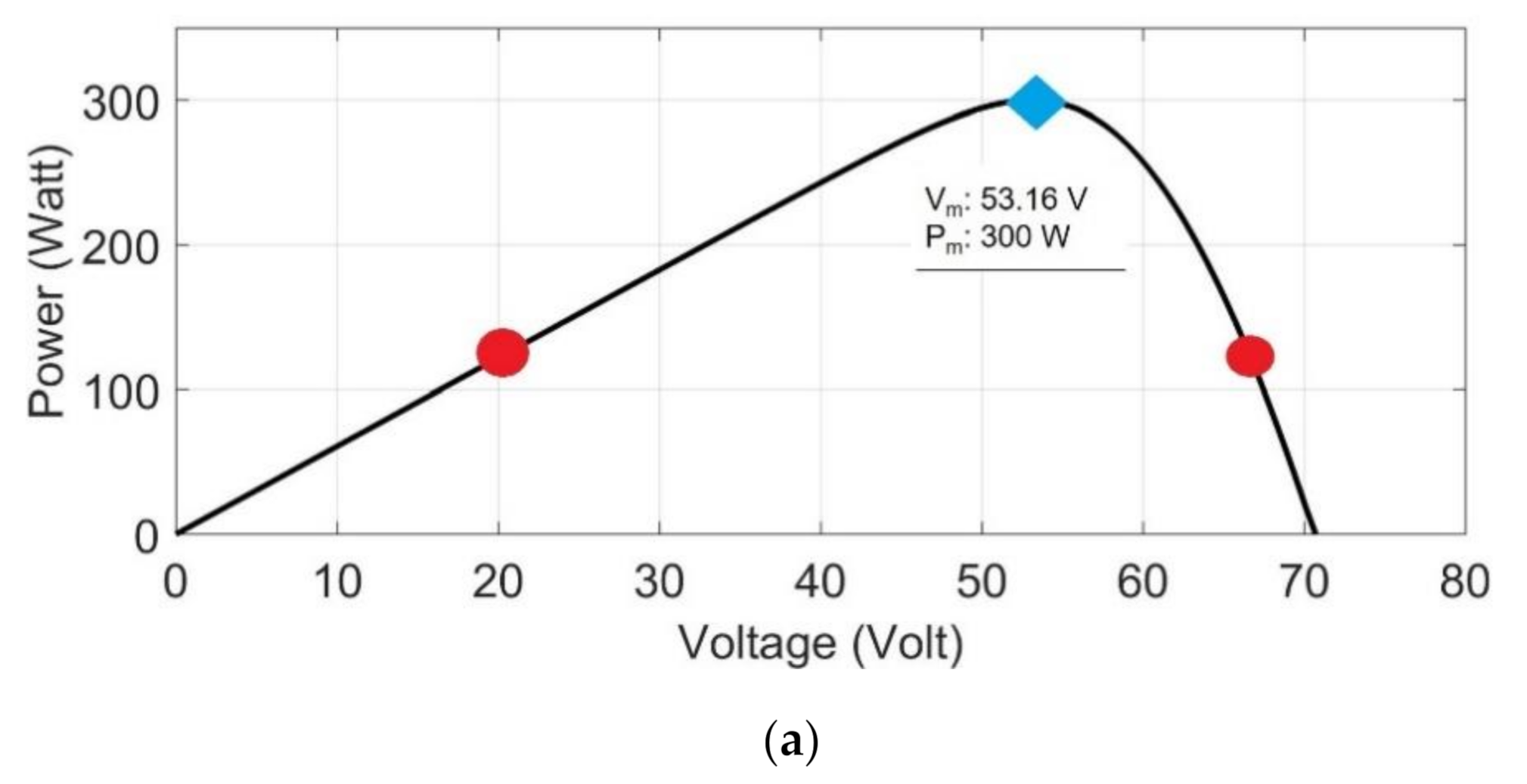
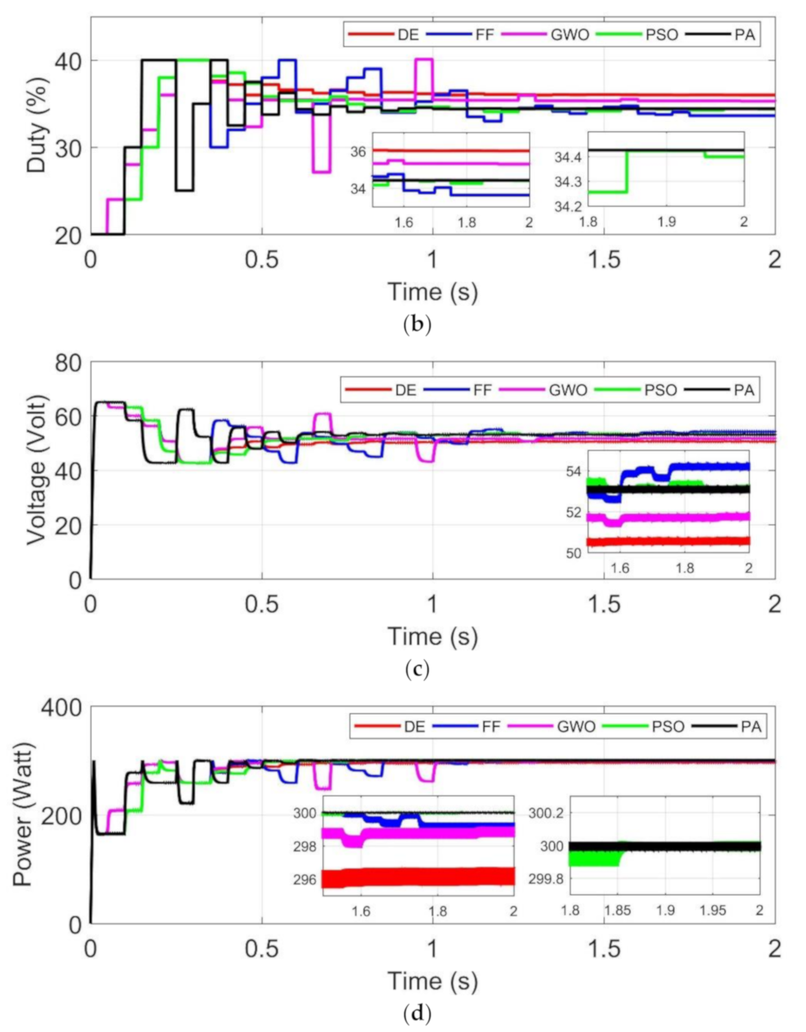
4.1. Uniform Irradiance Test
4.1.1. Test 1: Initial Particles at Left Side of MPP
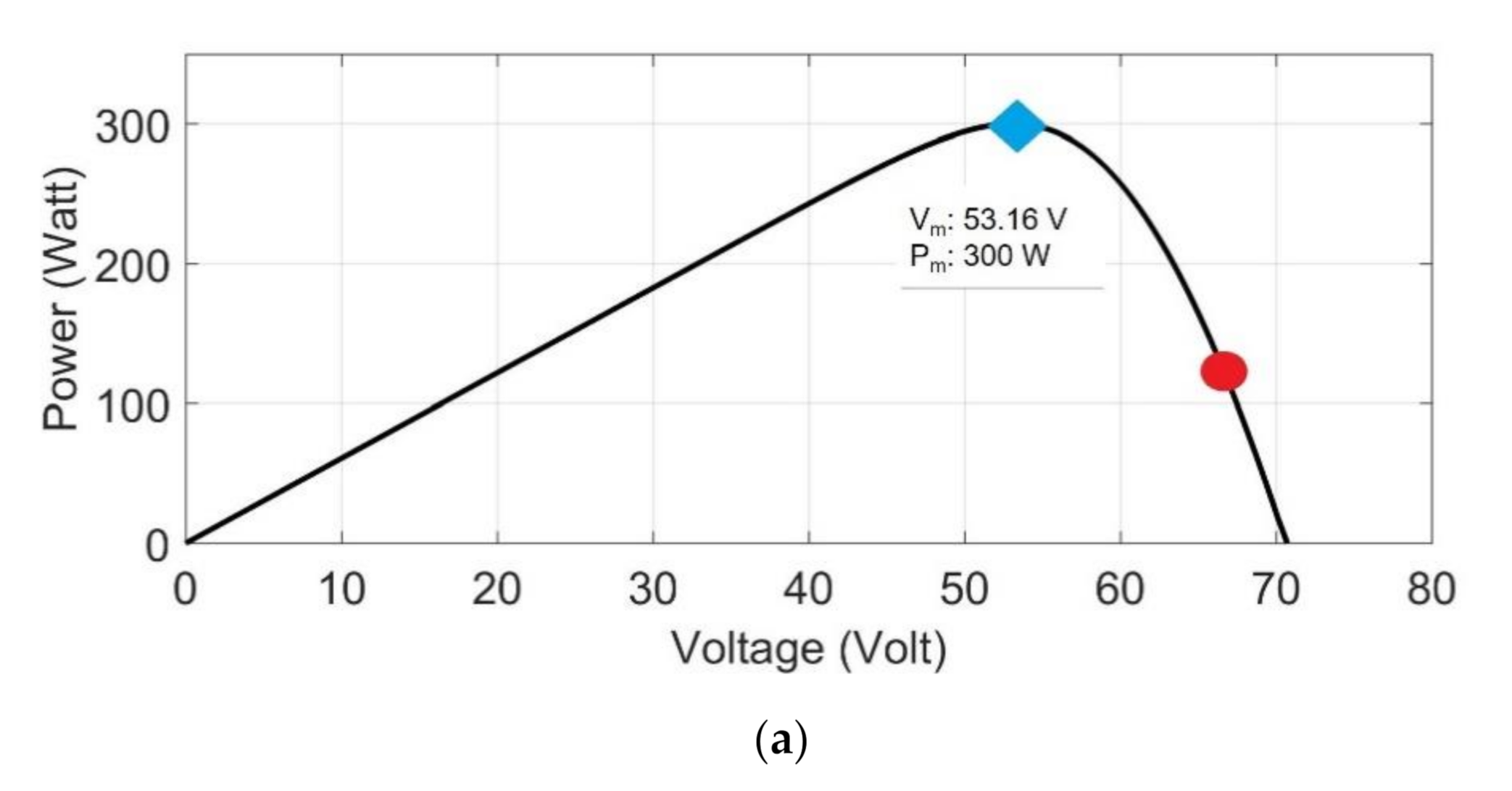
4.1.2. Test 2: Initial Particles at Right Side MPP
4.1.3. Test 3: Initial Particles at Surrounding MPP
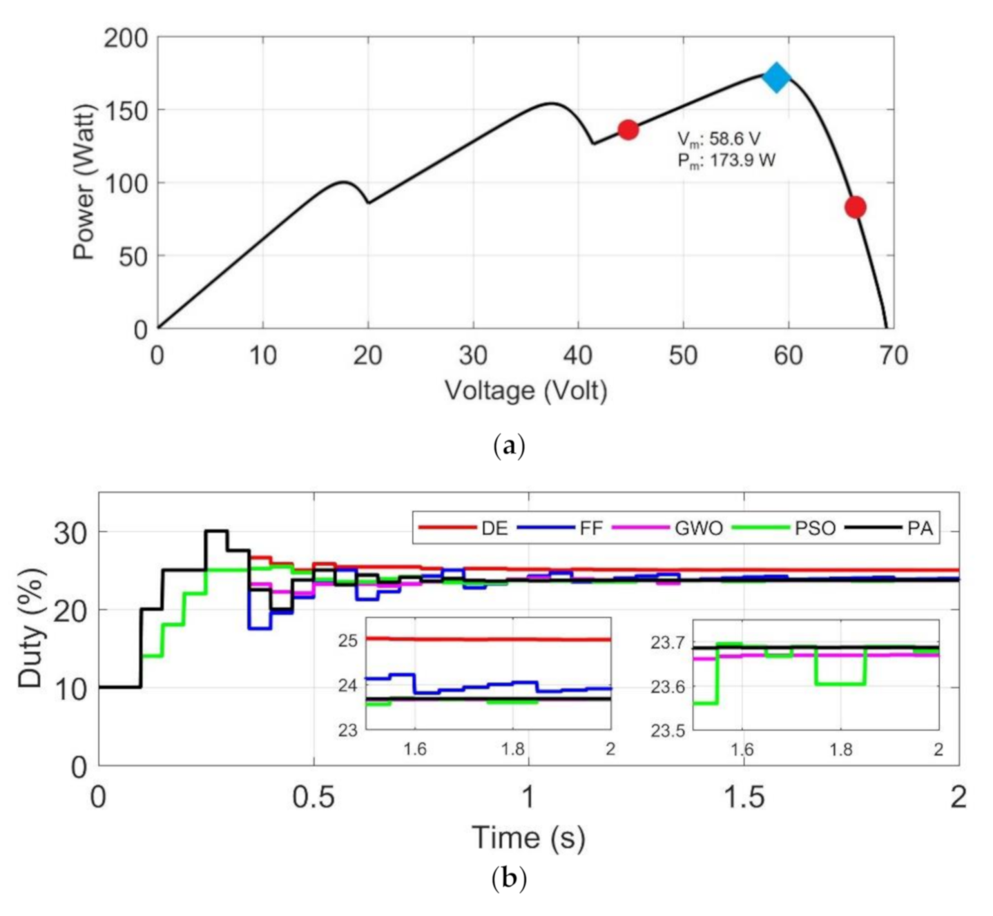
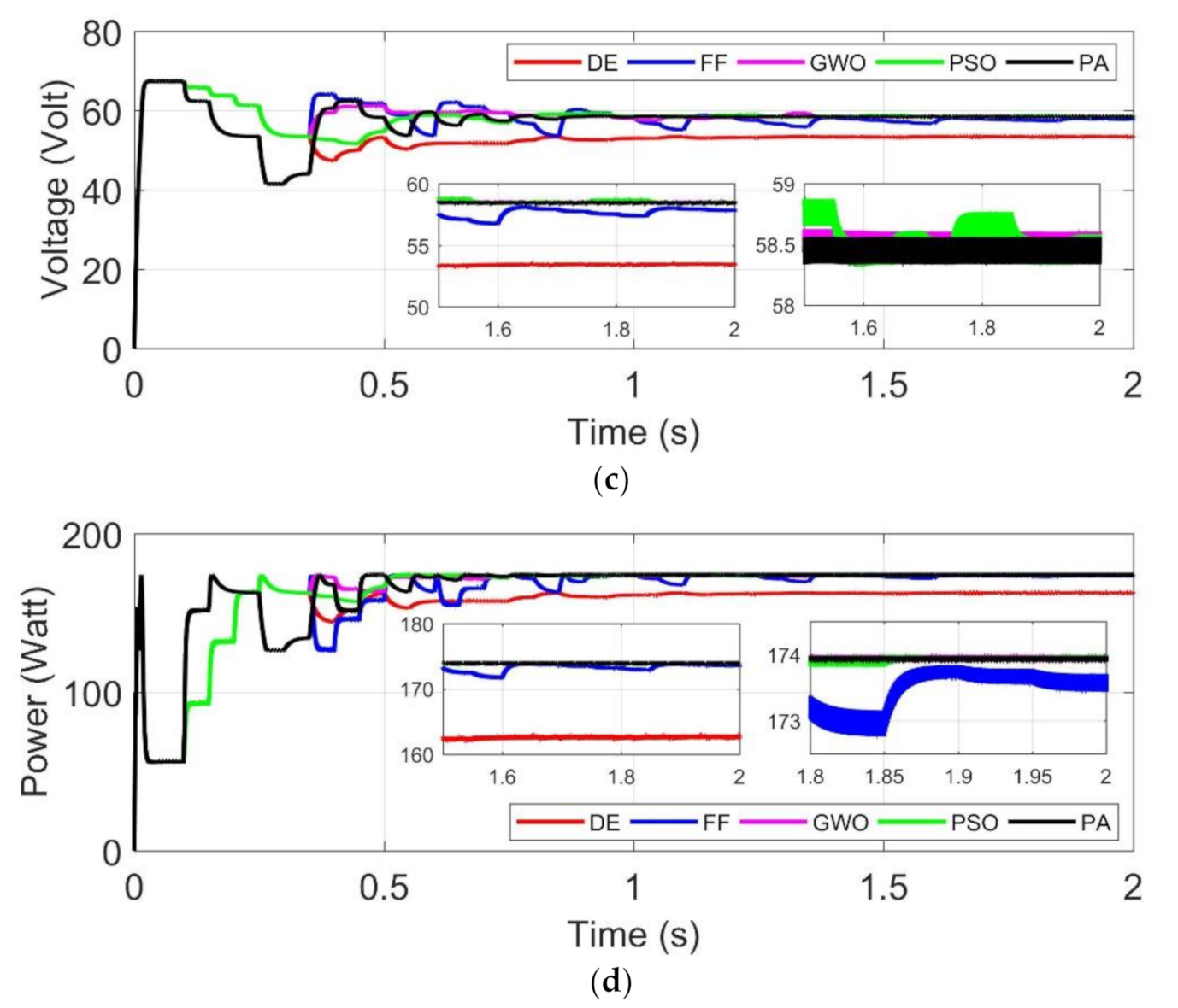
4.2. Partial Shading
4.2.1. Test 4: GMPP at Right Side
4.2.2. Test 5: GMPP Is Near Initial Particles Location
4.2.3. Test 6: GMPP Is Far from Initial Positions of Particles
5. Performance Evaluation
6. Conclusions
Author Contributions
Funding
Institutional Review Board Statement
Informed Consent Statement
Data Availability Statement
Conflicts of Interest
References
- Femia, N.; Giovanni, P.; Giovanni, S.; Massimo, V. A technique for improving P&O MPPT performances of double-stage grid-connected photovoltaic systems. IEEE Trans. Ind. Electron. 2009, 56, 4473–4482. [Google Scholar]
- Hung, H.I.; Shih, S.-F.; Hsieh, J.-H.; Hsieh, G.-C. A study of high-frequency photovoltaic pulse charger for lead-acid battery guided by PI-INC MPPT. In Proceedings of the International Conference on Renewable Energy Research and Applications (ICRERA), Nagasaki, Japan, 11–14 November 2012; IEEE: New York, NY, USA, 2012. [Google Scholar]
- Luigi, P.; Rizzo, R. Adaptive perturb and observe algorithm for photovoltaic maximum power point tracking. IET Renew. Power Gener. 2010, 4, 317–328. [Google Scholar]
- Fathabadi, H. Novel fast dynamic MPPT (maximum power point tracking) technique with the capability of very high accurate power tracking. Energy 2016, 94, 466–475. [Google Scholar] [CrossRef]
- Macaulay, J.; Zhou, Z. A fuzzy logical-based variable step size P&O MPPT algorithm for photovoltaic system. Energies 2018, 11, 1340. [Google Scholar]
- Alik, R.; Jusoh, A. Modified Perturb and Observe (P&O) with checking algorithm under various solar irradiation. Sol. Energy 2017, 148, 128–139. [Google Scholar]
- Tey, K.S.; Mekhilef, S. Modified incremental conductance MPPT algorithm to mitigate inaccurate responses under fast-changing solar irradiation level. Sol. Energy 2014, 101, 333–342. [Google Scholar] [CrossRef]
- Teng, J.; Huang, W.; Hsu, T.; Wang, C. Novel and Fast Maximum Power Point Tracking for Photovoltaic Generation. IEEE Trans. Ind. Electron. 2016, 63, 4955–4966. [Google Scholar] [CrossRef]
- Mahmoud, Y.; El-Saadany, E.F. Fast Power-Peaks Estimator for Partially Shaded PV Systems. IEEE Trans. Energy Convers. 2016, 31, 206–217. [Google Scholar] [CrossRef]
- Moshksar, E.; Ghanbari, T. A model-based algorithm for maximum power point tracking of PV systems using exact analytical solution of single-diode equivalent model. Sol. Energy 2018, 162, 117–131. [Google Scholar] [CrossRef]
- Rizzo, S.A.; Scelba, G. ANN based MPPT method for rapidly variable shading conditions. Appl. Energy 2015, 145, 124–132. [Google Scholar] [CrossRef]
- Schill, C.; Brachmann, S.; Koehl, M. Impact of soiling on IV-curves and efficiency of PV-modules. Sol. Energy 2015, 112, 259–262. [Google Scholar] [CrossRef]
- Ramli, M.A.M.; Prasetyono, E.; Wicaksana, R.W.; Windarko, N.A.; Sedraoui, K.; Al-Turkia, Y.A. On the investigation of photovoltaic output power reduction due to dust accumulation and weather conditions. Renew. Energy 2016, 99, 836–844. [Google Scholar] [CrossRef]
- Mamun, M.A.A.; Hasanuzzaman, M.; Selvaraj, J. Experimental investigation of the effect of partial shading on photovoltaic performance. IET Renew. Power Gener. 2017, 11, 912–921. [Google Scholar] [CrossRef]
- El-Baz, W.; Tzscheutschler, P.; Wagner, U. Day-ahead probabilistic PV generation forecast for buildings energy management systems. Sol. Energy 2018, 171, 478–490. [Google Scholar] [CrossRef]
- Corizzo, R.; Ceci, M.; Japkowicz, N. Anomaly Detection and Repair for Accurate Predictions in Geo-distributed Big Data. Big Data Res. 2019, 16, 18–35. [Google Scholar] [CrossRef]
- Ceci, M.; Malerba, R.C.D.; Rashkovska, A. Spatial autocorrelation and entropy for renewable energy forecasting. Data Min. Knowl. Discov. 2019, 33, 698–729. [Google Scholar] [CrossRef]
- Udenze, P.; Hu, Y.; Wen, H.; Ye, X.; Ni, K. A Reconfiguration Method for Extracting Maximum Power from Non-Uniform Aging Solar Panels. Energies 2018, 11, 2743. [Google Scholar] [CrossRef] [Green Version]
- Chandra, S.; Gaur, P. Radial Basis Function Neural Network Technique for Efficient Maximum Power Point Tracking in Solar Photo-Voltaic System. Procedia Comput. Sci. 2020, 167, 2354–2363. [Google Scholar] [CrossRef]
- Pathak, P.K.; Yadav, A.K. Design of battery charging circuit through intelligent MPPT using SPV system. Sol. Energy 2019, 178, 79–89. [Google Scholar] [CrossRef]
- Lin, W.; Hong, C.; Chen, C. Neural-Network-Based MPPT Control of a Stand-Alone Hybrid Power Generation System. IEEE Trans. Power Electron. 2011, 26, 3571–3581. [Google Scholar] [CrossRef]
- Liu, Y.-H.; Liu, C.-L.; Huang, J.-W.; Chen, J.-H. Neural-network-based maximum power point tracking methods for photovoltaic systems operating under fast changing environments. Sol. Energy 2013, 89, 42–53. [Google Scholar] [CrossRef]
- Yilmaz, U.; Kircay, A.; Borekci, S. PV system fuzzy logic MPPT method and PI control as a charge controller. Renew. Sustain. Energy Rev. 2018, 81, 994–1001. [Google Scholar] [CrossRef]
- Loukil, K.; Abbes, H.; Abid, H.; Abid, M.; Toumi, A. Design and implementation of reconfigurable MPPT fuzzy controller for photovoltaic systems. Ain Shams Eng. J. 2020, 11, 319–328. [Google Scholar] [CrossRef]
- Tang, S.; Sun, Y.; Chen, Y.; Zhao, Y.; Yang, Y.; Szeto, W. An Enhanced MPPT Method Combining Fractional-Order and Fuzzy Logic Control. IEEE J. Photovolt. 2017, 7, 640–650. [Google Scholar] [CrossRef]
- Nabipour, M.; Razaz, M.; Seifossadat, S.; Mortazavi, S.S. A new MPPT scheme based on a novel fuzzy approach. Renew. Sustain. Energy Rev. 2017, 74, 1147–1169. [Google Scholar] [CrossRef]
- Črepinšek, M.; Liu, S.-H.; Mernik, M. Exploration and exploitation in evolutionary algorithms: A survey. ACM Comput. Surv. 2013, 45, 1–33. [Google Scholar] [CrossRef]
- Priyadarshi, N.; Ramachandaramurthy, V.; Padmanaban, S.; Azam, F. An Ant Colony Optimized MPPT for Standalone Hybrid PV-Wind Power System with Single Cuk Converter. Energies 2019, 12, 167. [Google Scholar] [CrossRef] [Green Version]
- Titri, S.; Larbes, C.; Youcef-Toumi, K.; Benatchba, K. A new MPPT controller based on the Ant Colony Optimization Algorithm for Photovoltaic Systems under Partial Shading Conditions. Appl. Soft Comput. 2017, 58, 465–479. [Google Scholar] [CrossRef]
- Kinattingal, S.; Simon, S.P.; Nayak, P.S.R. MPPT in PV systems using ant colony optimisation with dwindling population. IET Renew. Power Gener. 2020, 14, 1105–1112. [Google Scholar]
- Ahmed, J.; Salam, Z. A soft computing MPPT for PV system based on Cuckoo Search algorithm. In Proceedings of the 4th International Conference on Power Engineering, Energy and Electrical Drives, Istanbul, Turkey, 13–17 May 2013; IEEE: New York, NY, USA, 2013. [Google Scholar]
- Mosaad, M.I.; El-Raouf, M.O.; Al-Ahmar, M.A.; Banakher, F.A. Maximum Power Point Tracking of PV system Based Cuckoo Search Algorithm; review and comparison. Energy Procedia 2019, 162, 117–126. [Google Scholar] [CrossRef]
- Basha, C.H.; Bansal, V.; Rani, C.; Brisilla, R.M.; Odofin, S. Development of Cuckoo Search MPPT Algorithm for Partially Shaded Solar PV SEPIC Converter. In Soft Computing for Problem Solving. Advances in Intelligent Systems and Computing; Springer: Singapore, 2020; pp. 727–736. [Google Scholar]
- Sundareswaran, K.; Peddapati, S.; Palani, S. MPPT of PV Systems under Partial Shaded Conditions through a Colony of Flashing Fireflies. IEEE Trans. Energy Convers. 2014, 29, 463–472. [Google Scholar]
- Huang, Y.-P.; Ye, C.-E.; Chen, X. A Modified Firefly Algorithm with Rapid Response Maximum Power Point Tracking for Photovoltaic Systems under Partial Shading Conditions. Energies 2018, 11, 2284. [Google Scholar] [CrossRef] [Green Version]
- Zhang, M.; Chen, Z.; Wei, L. An Immune Firefly Algorithm for Tracking the Maximum Power Point of PV Array under Partial Shading Conditions. Energies 2019, 12, 3083. [Google Scholar] [CrossRef] [Green Version]
- Chaurasia, G.S.; Singh, A.K.; Agrawal, S.; Sharma, N.K. A meta-heuristic firefly algorithm based smart control strategy and analysis of a grid connected hybrid photovoltaic/wind distributed generation system. Sol. Energy 2017, 150, 265–274. [Google Scholar] [CrossRef]
- Ebrahim, M.; Osama, A.; Kotb, K.M.; Bendary, F. Whale inspired algorithm based MPPT controllers for grid-connected solar photovoltaic system. Energy Procedia 2019, 162, 77–86. [Google Scholar] [CrossRef]
- Qais, M.H.; Hasanien, H.M.; Alghuwainem, S. Enhanced whale optimization algorithm for maximum power point tracking of variable-speed wind generators. Appl. Soft Comput. 2020, 86, 105937. [Google Scholar] [CrossRef]
- Tey, K.S.; Mekhilef, S.; Seyedmahmoudian, M.; Horan, B.; Oo, A.T.; Stojcevski, A. Improved Differential Evolution-Based MPPT Algorithm Using SEPIC for PV Systems Under Partial Shading Conditions and Load Variation. IEEE Trans. Ind. Inform. 2018, 14, 4322–4333. [Google Scholar] [CrossRef]
- NaimTajuddin, M.F.; Ayob, S.M.; SazliSaad, Z. Evolutionary based maximum power point tracking technique using differential evolution algorithm. Energy Build. 2013, 67, 245–252. [Google Scholar]
- Ramli, M.A.; Ishaque, K.; Jawaid, F.; Al-Turki, Y.A.; Salam, Z. A modified differential evolution based maximum power point tracker for photovoltaic system under partial shading condition. Energy Build. 2015, 103, 175–184. [Google Scholar] [CrossRef]
- Mohanty, S.; Subudhi, B.; Ray, P.K. A Grey Wolf-Assisted Perturb & Observe MPPT Algorithm for a PV System. IEEE Trans. Energy Convers. 2017, 32, 340–347. [Google Scholar]
- Eltamaly, A.M.; Farh, H.M. Dynamic global maximum power point tracking of the PV systems under variant partial shading using hybrid GWO-FLC. Sol. Energy 2019, 177, 306–316. [Google Scholar] [CrossRef]
- Mirza, A.F.; Mansoor, M.; Ling, Q.; Yin, B.; Javed, M.Y. A Salp-Swarm Optimization based MPPT technique for harvesting maximum energy from PV systems under partial shading conditions. Energy Convers. Manag. 2020, 209, 112625. [Google Scholar] [CrossRef]
- Farh, H.M.H.; Othman, M.F.; Eltamaly, A.M. Maximum power extraction from grid-connected PV system. In Proceedings of the 2017 Saudi Arabia Smart Grid (SASG), Jeddah, Saudi Arabia, 12–14 December 2017; IEEE: New York, NY, USA, 2017. [Google Scholar]
- Ram, J.P.; Rajasekar, N. A new robust, mutated and fast tracking LPSO method for solar PV maximum power point tracking under partial shaded conditions. Appl. Energy 2017, 201, 45–59. [Google Scholar]
- Eltamaly, A.M.; Al-Saud, M.; Abokhalil, A.G.; Farh, H.M. Simulation and experimental validation of fast adaptive particle swarm optimization strategy for photovoltaic global peak tracker under dynamic partial shading. Energy Rev. 2020, 124, 109719. [Google Scholar] [CrossRef]
- Peng, B.; Ho, K.; Liu, Y. A Novel and Fast MPPT Method Suitable for Both Fast Changing and Partially Shaded Conditions. IEEE Trans. Ind. Electron. 2018, 65, 3240–3251. [Google Scholar] [CrossRef]
- Mirza, A.F.; Ling, Q.; Javed, M.Y.; Mansoor, M. Novel MPPT techniques for photovoltaic systems under uniform irradiance and Partial shading. Sol. Energy 2019, 184, 628–648. [Google Scholar] [CrossRef]
- Shams, I.; Mekhilef, D.S.; Soon, T.K. Maximum Power Point Tracking using Modified Butterfly Optimization Algorithm for Partial Shading, Uniform Shading and Fast Varying Load Conditions. IEEE Trans. Power Electron. 2020. [Google Scholar] [CrossRef]
- Kumar, N.; Hussain, I.; Singh, B.; Panigrahi, B.K. Rapid MPPT for Uniformly and Partial Shaded PV System by Using JayaDE Algorithm in Highly Fluctuating Atmospheric Conditions. IEEE Trans. Ind. Inform. 2017, 13, 2406–2416. [Google Scholar] [CrossRef]
- Li, L.; Chen, Y.; Liu, H.; Tang, W.; Liu, M.; Wu, J.; Li, Z. A Multi-Producer Group-Search-Optimization Method-Based Maximum-Power-Point-Tracking for Uniform and Partial Shading Condition. IEEE Access 2020, 8, 184688–184696. [Google Scholar] [CrossRef]
- Veerasamy, B.; Thelkar, A.R.; Ramu, G.; Takeshita, T. Efficient MPPT control for fast irradiation changes and partial shading conditions on PV systems. In Proceedings of the 2016 IEEE International Conference on Renewable Energy Research and Applications (ICRERA), Birmingham, UK, 20–23 November 2016; IEEE: New York, NY, USA, 2016. [Google Scholar]
- Farayola, A.M.; Hasan, A.N.; Ali, A.; Twala, B. Distributive MPPT Approach Using ANFIS and Perturb&Observe Techniques Under Uniform and Partial Shading Conditions. In Artificial Intelligence and Evolutionary Computations in Engineering Systems; Springer: Singapore, 2018; pp. 27–37. [Google Scholar]
- Ostadrahimi, A.; Mahmoud, Y. Novel Spline-MPPT Technique for Photovoltaic Systems under Uniform Irradiance and Partial Shading Conditions. IEEE Trans. Sustain. Energy 2021, 12, 524–532. [Google Scholar] [CrossRef]
- Rhouma, M.B.; Gastli, A.; Brahim, L.B.; Touati, F.; Benammar, M. A simple method for extracting the parameters of the PV cell single-diode model. Renew. Energy 2017, 113, 885–894. [Google Scholar] [CrossRef]
- Patel, H.; Agarwal, V. MATLAB-Based Modeling to Study the Effects of Partial Shading on PV Array Characteristics. IEEE Trans. Energy Convers. 2008, 23, 302–310. [Google Scholar] [CrossRef]
- Hart, D.W. Power Electronics; Tata McGraw-Hill Education: New York, NY, USA, 2011. [Google Scholar]


| No. | Identified Existing Issues from the Literature | The Key Contributions of the Proposed Algorithm |
|---|---|---|
| 1. |
|
|
| 2. |
|
|
| 3. |
|
|
| 4. |
|
|
| 5. |
|
|
| No. | Parameters | Variable | Value |
|---|---|---|---|
| 1. | Number of Cells | 36 | |
| 2. | Maximum Power | Pm | 100 W |
| 3. | Voltage at Pm | Vm | 17.6 V |
| 4. | Current at Pm | Im | 5.69 A |
| 5. | Open-Circuit Voltage | Voc | 22.6 V |
| 6. | Short-Circuit Current | 6.09 A | |
| 7. | Shunt Resistance | 134.0754 Ohm | |
| 8. | Series Resistance | 0.286 Ohm | |
| 9. | Light Intensity | 1000 W/m2 | |
| 10. | Ambient Temperature | 25 °C | |
| 11. | Diode saturation current | 8.99 × 10⁻⁹ A | |
| 12. | Ideality factor | 1.25052 | |
| 13. | Temperature coefficient | 0.003958 A/°C | |
| 14. | Bandgap energy | 1.12 eV |
| No. | Component/Parameter | Label | Value |
|---|---|---|---|
| 1 | Switching frequency | 10 kHz | |
| 2 | Inductor | 87 µH | |
| 3 | Capacitor | 43 µF | |
| 4 | Load resistor | 1.2 Ω |
| Case | Irradiance (W/m2) | GMPP | Dstart | |||||
|---|---|---|---|---|---|---|---|---|
| Test | PV1 | PV2 | PV3 | Position | Pm (W) | Vm (V) | Dm (%) | D1 to Dn (%) |
| 4 | 1000 | 500 | 700 | Right | 173.9 W | 58.6 V | 23% | 10 to 25% |
| 5 | 1000 | 800 | 300 | Middle | 171.9 W | 36.9 V | 37% | 10 to 25% |
| 6 | 100 | 150 | 800 | Left | 81.3 W | 17.9 V | 53% | 10 to 25% |
| Test NO/Algorithm | Tracking Time (s) | Settling Time (s) | Power Tracking (W) | Power Tracking Acc. (%) | Energy Harvesting (Ws) | Energy Tracking Acc (%) |
|---|---|---|---|---|---|---|
| Test 1 | 300.0 | 100.00 | 600.0 | 100.00 | ||
| DE | - | - | 76.7 | 25.57 | 146.8 | 24.47 |
| FF | - | - | 76.5 | 25.50 | 72.7 | 12.12 |
| PSO | 0.44 | - | 299.9 | 99.97 | 382.2 | 63.70 |
| GWO | - | - | 92.3 | 30.77 | 169.6 | 28.27 |
| PA | 0.39 | 0.79 | 299.9 | 99.97 | 523.6 | 87.27 |
| Test 2 | 300.0 | 100.000 | 600.0 | 100.00 | ||
| DE | - | - | 256.7 | 85.57 | 466.5 | 77.75 |
| FF | - | - | 84.5 | 28.17 | 213.2 | 35.53 |
| PSO | 1.11 | 1.72 | 299.9 | 99.97 | 521.7 | 86.95 |
| GWO | - | - | 286.7 | 95.57 | 477.5 | 79.58 |
| PA | 0.61 | 0.82 | 299.9 | 99.97 | 550.7 | 91.78 |
| Test 3 | 300.0 | 100.00 | 600.0 | 100.00 | ||
| DE | - | - | 295.7 | 98.57 | 570.6 | 95.10 |
| FF | 1.19 | - | 299.9 | 99.97 | 568.1 | 94.68 |
| PSO | 1.01 | 1.92 | 299.9 | 99.97 | 570.6 | 95.10 |
| GWO | 0.60 | 1.62 | 298.5 | 99.50 | 572.4 | 95.40 |
| PA | 0.61 | 1.11 | 299.9 | 99.97 | 573.4 | 95.57 |
| Test 4 | 173.9 | 100.00 | 347.8 | 100.00 | ||
| DE | - | - | 163.4 | 93.96 | 305.1 | 87.72 |
| FF | 0.49 | - | 171.7 | 98.73 | 322.2 | 92.64 |
| PSO | 0.51 | - | 172.3 | 99.08 | 324.3 | 93.24 |
| GWO | 0.77 | 1.36 | 172.9 | 99.42 | 326.4 | 93.85 |
| PA | 0.45 | 0.85 | 172.9 | 99.42 | 327.3 | 94.11 |
| Test 5 | 171.9 | 100.00 | 343.8 | 100.00 | ||
| DE | - | - | 133.2 | 77.49 | 244.5 | 71.12 |
| FF | - | - | 103.2 | 60.03 | 191.4 | 55.67 |
| PSO | - | - | 113.6 | 66.08 | 216.4 | 62.94 |
| GWO | 1.12 | 1.72 | 170.9 | 99.42 | 298.3 | 86.77 |
| PA | 0.41 | 1.02 | 170.9 | 99.42 | 316.7 | 92.12 |
| Test 6 | 81.3 | 100.00 | 162.6 | 100.00 | ||
| DE | - | - | 35.7 | 43.91 | 70.2 | 43.17 |
| FF | - | - | 24.8 | 30.50 | 51.3 | 31.55 |
| PSO | - | - | 31.2 | 38.38 | 60.1 | 36.96 |
| GWO | 1.31 | 1.62 | 80.9 | 99.51 | 128.3 | 78.91 |
| PA | 0.52 | 0.87 | 80.9 | 99.51 | 140.3 | 86.29 |
Publisher’s Note: MDPI stays neutral with regard to jurisdictional claims in published maps and institutional affiliations. |
© 2021 by the authors. Licensee MDPI, Basel, Switzerland. This article is an open access article distributed under the terms and conditions of the Creative Commons Attribution (CC BY) license (http://creativecommons.org/licenses/by/4.0/).
Share and Cite
Windarko, N.A.; Nizar Habibi, M.; Sumantri, B.; Prasetyono, E.; Efendi, M.Z.; Taufik. A New MPPT Algorithm for Photovoltaic Power Generation under Uniform and Partial Shading Conditions. Energies 2021, 14, 483. https://0-doi-org.brum.beds.ac.uk/10.3390/en14020483
Windarko NA, Nizar Habibi M, Sumantri B, Prasetyono E, Efendi MZ, Taufik. A New MPPT Algorithm for Photovoltaic Power Generation under Uniform and Partial Shading Conditions. Energies. 2021; 14(2):483. https://0-doi-org.brum.beds.ac.uk/10.3390/en14020483
Chicago/Turabian StyleWindarko, Novie Ayub, Muhammad Nizar Habibi, Bambang Sumantri, Eka Prasetyono, Moh. Zaenal Efendi, and Taufik. 2021. "A New MPPT Algorithm for Photovoltaic Power Generation under Uniform and Partial Shading Conditions" Energies 14, no. 2: 483. https://0-doi-org.brum.beds.ac.uk/10.3390/en14020483