Article

Investigating the Asymmetric Effect of Economic Growth on Environmental Quality in the Next 11 Countries

by
Gideon Kwaku Minua Ampofo
1,
Jinhua Cheng
1,*,
Edwin Twum Ayimadu
2 and
Daniel Akwasi Asante
1
1
School of Economics and Management Sciences, China University of Geosciences, Wuhan 430074 China
2
Department of Land and Natural Resource, China University of Geosciences, Wuhan 430074, China
*
Author to whom correspondence should be addressed.
Submission received: 20 December 2020 / Revised: 13 January 2021 / Accepted: 15 January 2021 / Published: 18 January 2021

Abstract

:
This study investigates the asymmetric cointegration and causal relationships between economic growth, carbon emissions, and energy consumption in the next eleven (11) countries over the period 1972–2013. The nonlinear autoregressive distributed lag (NARDL) bounds testing approach and nonpragmatic Granger causality tests are employed. This research’s empirical results have entrenched vital relationships that have significant policy implications. We affirm nonlinear cointegration among the variables in Bangladesh, Iran, Turkey, and Vietnam. The long-run asymmetric effect outcomes indicate a definite boom in economic growth, significantly increases carbon emission in Turkey, and a decline in Vietnam. Additionally, a positive shock to energy consumption significantly increases the carbon emission in Bangladesh, Iran, and Turkey, but a decrease in emissions in Vietnam. Findings from the Wald test reveal a long-run asymmetric effect between carbon emission and economic growth in Bangladesh, Iran, and Vietnam, and for Iran, an asymmetric short-run impact. Long-run and short-run asymmetric effects between carbon emission and energy consumption in Bangladesh and Iran. In terms of asymmetric causality results, bidirectional causality between carbon emission and economic growth was noted in Bangladesh and Turkey, and a unidirectional causality from economic growth to carbon emission in Egypt and South Korea. Energy consumption causes carbon emission in Bangladesh, Egypt, Pakistan, South Korea, and not vice versa. We determined a bidirectional asymmetric causality relationship between carbon emission and energy consumption in Vietnam and a unidirectional causality link from carbon emissions to Turkey’s energy consumption.

1. Introduction

Globalization, which has been the hallmark of this current era, has had an unprecedented political, social, cultural, and economic impact on the world. It has led to some form of competition among developed and developing countries alike as they try to economically outperform each other since economic growth is deemed the penultimate goal by policymakers for sustainable development. Moreover, third world economies are frantically trying to induce human capital formation and economic activities while maintaining their comparative advantage in the globalized world. According to [1], the combination of labor, capital resources, other production inputs, and mainly human activities are responsible for growth globally. However, it is prudent to add that greenhouse gas (GHG) emissions have been on the ascending as a result of industrial growth in both first and third world countries. Notably, carbon emissions contribute to a more significant portion of GHG’s, which are more probably linked to climate change [2,3,4]. Moreover, the concentration of CO2 emission has increased by 45% in the past 130 years [5].
It is widely known in economic circles that sustainable development is a prerequisite to liberate an economy from backwardness, reducing poverty and instigating growth and development. Therefore, developing countries in the 21st century are embarking on aggressive economic growth and urbanization. The surge in their demand for energy and its consumption in recent years, however, can never go unnoticed. If the role machines played in the transition to new manufacturing processes in Europe and the United States was considered the game-changer during the industrial revolution, then energy was its driving force. Energy is an indispensable factor of production [6]. In this perspective, it is essential to note that, despite economic growth in developing countries is on the ascendance, its toll on natural resources and contribution to greenhouse gasses is alarming. All production categorically involves the conversion or metamorphosis of matter in some way using energy. Energy as a factor of production must be integrated into materials, machines, and the people who work them to be made useful; this provides the biophysical justification for treating capital, labor, and others as factors of production [7]. This proposes the efficient use of energy (i.e., the renewable or nonrenewable form). It is essential in the sense that carbon dioxide (CO2) emission, which goes hand in hand with increasing energy consumption, has an irreversible adverse impact on the environment if allowed to go unchecked. Furthermore, the Intergovernmental Panel on Climate Change [8] anticipated that GHG emissions would increase from 25% to 90% increased and energy-related CO2 emissions by 40–110% by the year 2030. The intricacies surrounding energy use and economic growth and their effects on carbon emissions have been unfolding into a severe topic among researchers [9,10].
To some extent, economic growth exerts pressure on environmental quality as boosting economic growth sabotage efforts aimed at either maintaining or improving environmental quality. The connection between economic growth, environmental quality, and energy consumption and how these entities affect one another has presented a challenging but intriguing topic of extensive academic research in energy economics literature [11] and [12]. As economies worldwide continue to strive to greater heights to the detriment of environmental quality, its impact on human life is alarming. For instance, an estimated 7,000,000 carbon emissions related deaths are recorded worldwide [13]. Interestingly, it has been uncovered that as much energy creation is imperative for industrialization in rising economies, for example, Africa; it has, however, shown many difficulties like air pollution [14]. The Intergovernmental Panel on Climate Change [15] asserted that, out of the numerous contributors to GHG, CO2 accounts for an estimated 76.7%, signaling the immense devastation effect CO2 will have on human life if allowed to go on unchecked. According to the International Energy Agency [16], to guard human life and wellbeing against profound climate change, an objective was developed under the Kyoto protocol in 1997. This was to lessen greenhouse gas emissions in advanced nations to 5.2% at some stage between 2008 and 2012. Nevertheless, the Kyoto Protocol was revised at the 2012 United Nations’ Climate Change Conference to be prolonged to the year 2020 [17,18].
Under the weight of directing environmental change, developing countries are confronted with an impasse of reducing GHG emissions and energy consumption or boosting economic growth [19,20,21,22] have indicated that if actions to resolve the issue of environmental change as a result of global warming are not taken, the consequences thereof will be an economic loss and environmental catastrophe. Therefore, introducing a consistent policy to sustain economic growth while addressing issues concerning CO2 emissions is paramount to economic development.
The next 11 countries, also known as N11 countries, include Egypt, Mexico, Bangladesh, Indonesia, Nigeria, Iran, Pakistan, Turkey, Vietnam, South Korea, and the Philippines: have developing markets that could turn out to be the world’s major economies [23]. According to [24], these countries account for around 8% of the overall gross domestic product (G.D.P.), justifying their growth potential. With the growth in N-11 economies comes increased energy consumption. As economies become more industry-intensive and less energy-efficient to enhance growth, environmental problems begin to arise J.M.K.C. Donev et al. (2020). N-11 countries, therefore, generate about 10% of the global CO2 emissions [25].
Several researchers have reviewed the nexus between economic growth, environmental pollution, energy consumption, and findings have been inconclusive. Although most macroeconomic variables constitute nonlinear characteristics, a substantial part of the existing research on modeling the economic growth-carbon emission nexus was executed in a linear structure that assumed a symmetric relationship using different time-series methods. The mixed results that were arrived at concerning the economic growth–carbon emission relationship could be due to the linearity assumptions. Using linear models may not be a suitable approach to exploring the link between economic growth and carbon emissions since it may offer misleading suggestions on such a relationship.
As shown in a recent study by [26,27], carbon emission response will differ depending on the level of economic growth. Our study adds to the current literature in numerous forms. This study also aims to buttress the potential asymmetric relationship between economic growth and carbon emission for the next 11 countries. To the best of the authors’ knowledge, this is the first study that examines the asymmetric relationship between economic growth and carbon emission in the next 11 countries using the nonlinear autoregressive distributed lag (NARDL) model.
Second, to study the possible nonlinear relation between economic growth, energy consumption, and carbon emission, we employ the nonlinear autoregressive distributed lag (N.A.R.D.L.) model proposed by [28] for the individual countries. We decompose the growth per capita into positive and negative changes. We also examine the asymmetric causality using the [29] nonlinear Granger causality in place of the extensively used [30] nonlinear causality test to assess the causal link between carbon emission and economic growth. Our decision to employ the [29] nonlinear Granger causality is because of the limitations pointed out by [29] in the [30] test that the null hypothesis of non-causality may be over rejected.
The remainder of this study is in the following format. Section 2 highlights the literature review focusing on previous related studies on energy consumption, economic growth, and carbon emission nexus. In Section 3, the sources of data and methodology employed are presented. Empirical results are shown in Section 4. Whiles Section 5 reports the conclusions drawn from the study with the main findings and corresponding policy recommendations.

2. Literature Review

Ever since the pioneering work of [31] on the EKC concept, which was named after [32] numerous empirical studies such [33,34,35,36] have examined the validity of an inverted “U” correlation between growth per capita and environmental contamination. With reference to the IEA 2016 report, human activities have increased greenhouse gas leading to global warming. An increase in greenhouse gas concentrations by 90% in 2014 originated from carbon dioxide emissions, and 68% of carbon dioxide emissions emanated from the energy sector. Therefore, in the energy sector, carbon dioxide emissions are generally produced by carbon oxidation in fuels, references [37,38] asserted that the consumption of energy critically affects the environment, and for that matter, these environmental issues impede economic growth.
Halicioglu, F. (2009) [17], who conducted his studies in Turkey found out that economic growth had a compelling impact in explaining the country’s carbon emission than energy consumption. Pao, H.-T and Tsai, C.-M (2011) [39] found a similar in Brazil. As mentioned earlier, a year before just this work, [40] in conducting studies about this phenomenon in the BRIC (Brazil, Russia, India and China) countries found that a short-run and long-run causal relationship exists between carbon emission, energy consumption, and economic growth. In the same year, [18] came out with similar results for Turkey. Mendum, R. and Njenga, M. (2018) [41] reiterated that there is a considerable usage of fossil fuel energy, contributing to environmental degradation. On the other hand, reference [42] acknowledged the existence of a significant correlation between energy economic growth and consumption.
Similarly, [37] advocated that South Africa has to lessen energy consumption to fewer carbon emissions. In Saudi Arabia, [43] found that huge energy consumption volatility negatively impacts oil G.D.P. and CO2 emission. IEA (2016) states that in 2014, electricity and heating had a combined carbon emission of 42.2%, with another 19% coming from construction and manufacturing. Paramati, S.R., Sinha A. and Dogan, E. [44] examined the impact of renewable energy and nonrenewable energy consumption on carbon emissions and economic growth in the next-11 countries. They reported that renewable energy consumption had reduced carbon emission significantly, but the same cannot be said about nonrenewable energy. Reference [45] disclosed that natural gas consumption had a positive knock-on effect on China and India’s carbon emission from 1952 to 2012. Table 1 presents a summary of recent related literature on empirical studies that examined the EKC hypothesis.

3. Material and Methods

3.1. Data Sources

This research investigated the influence of economic development and energy consumption on CO2 emissions in the next 11 countries by utilizing annual time series data from 1972 to 2013 obtained from the World Development Indicator (WDI, 2019-CD-ROM). The variables employed include economic growth (proxied by GDP per capita (constant 2010 US$), energy consumption (measured in kilogram (kg) of oil equivalent per capita), and carbon emissions (measured in metric tons per capita). The countries used for the study are the next 11 countries, and the timeframe was dictated by data availability. They include; Egypt, Bangladesh, South Korea, Mexico, Iran, Nigeria, Vietnam, Indonesia, Turkey, Pakistan, and the Philippines. To eliminate heteroscedasticity, energy consumption and GDP per capita series were transformed to logarithmic form.

3.2. Theoretical Framework and Methodology

This section presents a theoretical framework via which economic growth may affect a country’s carbon emission. Several studies have investigated this phenomenon known as the environmental Kuznets curve (EKC), which hypothesizes that countries experience an increase in environmental degradation during their early stages of development and a subsequent decline when economic growth at a certain threshold is attained.
Although there are differences in environmental quality relations, most researchers adopt standard endogenous variables and exogenous explanatory variables based on the stud’s focus. It is important to note that several possible factors influence carbon emission apart from economic growth and energy consumption. For instance [75,76,77,78,79] included trade openness in their model. Other empirical studies also included financial development to investigate its impact on environment quality ([19,76,78,80,81,82], population density is another factor that has been identified to influence carbon emission as reported by [77,83,84], in their studies). Furthermore, [85,86] added technology and capital y to their explanatory variables whiles analyzing the link between carbon emission and economic growth. The impact of globalization and oil prices on carbon emission was also investigated in studies conducted by [51,75]. Some recent studies also included resource rents in their model to define the correlation between resource extraction, revenue, and carbon emissions. Our choice of variables is partly influenced by availability of a complete time data series in all the next-11 countries. We decided not to include other demographic variables, which in some previous studies are normally included as weak regressors because they are of little interest concerning the objectives of our research.
Some previous studies have established that a capital increase positively affects environmental quality in the long-run [86]. In terms of trade openness, [79] reported from a panel analysis that, trade openness hinders environmental quality for low income and middle, high income and global panels but noted that the effect is not the same in the various groups of countries investigated. Mrabet, Z., AlSamara, M. and Jarallah, S.H. (2017) [75] also noted that trade openness negatively impacts ecological footprint in the long-run. Jalil, A. and Feridun, M (2011) [76] revealed that financial development leads to a decline in China’s environmental pollution, and similar findings were made by [82]. In contrast, [87] in their study, posited financial development takes place at the expense of environmental quality, consistent with findings of [88]; reference [81] who reported that an increase in financial development leads to a rise in carbon emission and so does not mitigate it. Onafowora, O.A. and Owoye, O. (2014) [77] found no unique relationship between population density and the environment. However, [83] found out that as Taiwan’s population grows, there is an upsurge in carbon emission consistent with what has been reported by [89] in another study. A major driving force behind an increase in carbon emission globally in the last two decades is population [84]. The type of technology used also determines the level of environmental degradation [85].
This study adopts the multivariate framework, which controls for energy consumption since economic growth and carbon emission depend on the degree of energy consumption; thus, energy consumption has a significant effect on these variables and consistently included in models of most previous studies (see [26,34,90,91]). Similar studies conducted using a trivariate framework from which inspiration was drawn for this study are captured in the literature review.
Following the recent empirical work by [26], it is possible to test the long-run nexus between carbon emission, economic growth, and energy consumption. The primary, extended model, therefore, takes the following functional form with all variables converted into logarithms:
l o g C O i , t   = α + α 1 l o g E G i , t + α i , t   l o g E C i , t + μ i , t
where i and t indicate countries and years, while log represents the natural logarithm. CO represents the carbon emission, EG denotes G.D.P. per capita, which we used as a measure of economic growth, and EC is energy consumption.
The nonlinear cointegration regression proposed by [28] specified as:
y t =   β + x t + +   β x t +   μ +
where β + and β are long term parameters of k x 1 vector of regressors x t , decomposed as:
x t =   x 0 +   x t + +   x t  
where x t + x t are the partial sums of positive (negative) change in x t as follows:
x t + = j = 1 t Δ x j + = j = 1 t max ( Δ x j , 0 )
x t = j = 1 t Δ x j = j = 1 t min ( Δ x j , 0 )
The N.A.R.D.L. (p, q) form of Equation (3), in the form of asymmetric error correction model (A.E.C.M.), can be specified as:
Δ C O t = α 0 + p C O t 1 + θ 1 + E G t 1 + + θ 2 E G t 1 + θ 3 + E C t 1 + + θ 4 E C t 1 + i = 1 p α 1 Δ C O t 1 + i = 0 q α 2 Δ E G t 1 + + i = 0 q α 3 Δ E G t 1 + i = 0 q α 4 Δ E C t 1 + + i = 0 q α 5 Δ E C t 1   + μ t
where i = 1, …, 5., α i signifies the short-run coefficients, and θ i represents the long-run coefficients. At this point, the short-run coefficients disclose the immediate impact of independent variables on dependent variables. On the other hand, long-run coefficients display the speed and reaction time of the adjustment towards an equilibrium level. The Wald test is applied to analyze the null hypothesis for short-run asymmetry ( α = α + = α ) and long-run asymmetry ( θ = θ + = θ ) for variables C O t ,   E G t ,   and   E C t , which represents carbon emission, energy consumption, and economic growth, respectively. The optimal lags p and q will be resolved by the Akaike information criterion (A.I.C.) for the dependent variable C O t and independent variables E G t   and   E C t . To decompose, the positive and negative sum of all independent variables are given in the manner as follows.
x t + = j = 1 t Δ x j + = j = 1 t max Δ x j , 0   a n d   x t = j = 1 t Δ x j = j 1 t m i n Δ x j , 0  
where x t denotes the independent variables, E G t   and   E C t .
Where θ + =     ρ β + and   θ =     ρ β . To establish cointegration in a nonlinear structure, the first two initial steps are similar to the A.R.D.L. bound testing technique, i.e., estimating Equation (6) using ordinary least square and conducting the joint null ( ρ = θ + =   θ = 0 ) hypothesis test. However, in nonlinear A.R.D.L., the Wald test is applied to examine the long-run ( θ + =   θ ) and short-run ( π + =   π ) asymmetries in the relationship.
In the framework of the asymmetric error correction model presented above, [28] proposed two test statistics, namely the t-BDM and F-PSS, for testing the existence or absence of a cointegration relationship. While the t-BDM tests the null of no cointegration H 0 :   ρ = 0 against the alternative hypothesis of cointegration H 1 :   ρ < 0 , the F-PSS tests the joint null of no cointegration H 0 :   ρ = θ + = θ = 0 against the alternative joint hypothesis of cointegration H 1 :   ρ = θ + = θ < 0 . As the asymptotic distribution of the t-BDM and F-PSS statistics is non-standard regardless of whether the variables are at a level I(0) or first difference I(1), the conclusion for cointegration is taken by assessing two groups of critical values, one of which assumes that all variables are I(1). It provides a bound covering with all possible categorizations of the variables. If the computed test statistics fall above the upper level of the bound, the null hypothesis ( H 0 ) is rejected, supporting cointegration. If the computed test statistics fall below the lower level of the bound, the null hypothesis ( H 0 ) cannot be rejected, which indicates that cointegration does not exist.
The equation below used to determine the asymmetric dynamic multiplier effects:
m h + = j = 0 h C O t + j E G t + , m h = j = 0 h C O t + j E G t , m h + = j = 0 h C O t + j E C t + , m h = j = 0 h C O t + j E C t , m h +
If h ,   m h + L m + and   m h L m . It indicates the asymmetric reaction of the exogenous variable to both positive and negative changes in endogenous variables. The dynamic modification from the initial equilibrium to the new equilibrium in system variables can be observed.
The nonparametric Diks–Panchenko causality test:
In 1969, Granger proposed a causality test to define the dependence relations between economic time series. According to this, if two variables { X t , Y t , t 1 } are strictly stationary, Y t Granger causes X t if past or current values of X contain additional information on future values of Y .
Suppose that X t l x = X t 1   X + 1 , , X t and Y t l y = Y t 1   y + 1 , , Y t are the delay vectors, where l X , l Y 1 .
Diks, C.; Panchenko (2006) [29] examine the null hypothesis that past observations of X t l x contain any additional information about Y t + 1 (beyond that in Y t l y ):
H 0 :   Y t + 1       X t l X   ;   Y t l Y   ~   Y t + 1     Y t l Y
The equation below represents the test statistic:
T n ε n =   n 1 n n 2   .   i ( f ^ . X , Z , Y X i , Z i , Y i f ^ . Y Y i f ^ . X , Y X i , Y i f ^ . Y , Z Y i , Z i )
where f X , Y , Z x , y , z is the joint probability density function. For l X = l Y = 1 and if ε n = C n β ( C > 0, 1 4 < β < 1 3 ) , [29] prove that the test statistic in Equation (2) satisfies the following:
n T n ε n q S n D N 0 , 1
where D denotes convergence in distribution and S n is an estimator of the asymptotic variance of T n . [29,92].

4. Main Results and Discussions

Table 2 presents the main descriptive statistics of 41-year carbon emission, energy consumption, and growth values for each country. As can be observed, the highest amount of carbon emission was 11.803 recorded in South Korea. In terms of energy consumption, South Korea and Egypt recorded the highest value, 8.566, while the maximum growth value of 10.073 was reported in South Korea.

4.1. Unit Root Test

We began by testing the stationary properties of energy consumption, carbon emission, and economic growth. We applied the Phillips–Perron (PP) test and the augmented Dickey–Fuller (ADF) test to approve that the variables are not integrated at the second level difference since the NARDL test disallows the use of I(2) variables. The augmented Dickey–Fuller (A.D.F.) [93] and Phillips–Perron (P.P.) [94] test results shown in Table 3 indicate that all the variables are stationary at the first difference and level, respectively. This indicates that the variables are not integrated at the second level difference.

4.2. Linear Cointegration Test

Table 4 presents the results of the maximum-likelihood Johansen’s cointegration between economic growth, energy consumption, and carbon emission in the N-11 countries. Since none of the parameters were significant at 5%, in most countries except Bangladesh and Vietnam, we ruled out cointegration between economic growth, energy consumption, and carbon emission in those countries. Apart from Bangladesh, the null hypothesis of no cointegration was not rejected in other countries. This might have arisen due to the long-run nonlinear cointegration between energy consumption, carbon emission, and economic growth to be established by employing nonlinearity tests.

4.3. Linear Granger Causality Results

We assessed the linear causality between carbon emission, energy consumption, and economic growth, using each country’s conventional linear Granger causality test. The null hypothesis of the analysis states that there was no Granger causality. Thus, there was no linear causal relationship between carbon emissions and the two independent variables (economic growth and energy consumption). In contrast, there existed a linear Granger causality between the variables as proposed by the alternative hypothesis. Table 5 presents the results of maximum-likelihood Johansen cointegration between the variables.
In Bangladesh’s case, we found no bidirectional causality betwixt carbon emissions and energy consumption; instead, we observed economic growth Granger, causing carbon emission. Furthermore, energy consumption and economic growth were found to Granger cause carbon emissions in Pakistan. In Egypt, a unidirectional causality was seen running from carbon emission to economic growth. Concerning the Philippines, we failed to reject the null hypothesis of no Granger causality between our variables at all levels of significance. We confirmed a unidirectional Granger causality linkage running from energy consumption and economic growth to carbon emissions in Indonesia and South Korea. For Iran, we mentioned that economic growth Granger causes carbon emissions at a 5% level of significance. However, there was no significant causality that existed from energy consumption to carbon emissions. For Turkey, we failed to reject the null hypothesis of no Granger causality between our variables at all levels of significance. We rejected the null hypothesis of economic growth, not Granger causing carbon emission at a 5% significance level for Mexico. Results for Vietnam show a bidirectional Granger causality betwixt carbon emission and energy consumption and a unidirectional causality running from economic growth to carbon emission. The results also point out that there was no causal relationship between the variables for Nigeria.

4.4. B.D.S. Test

In examining the likelihood of nonlinear dependence between energy consumption and G.D.P. per capita, we utilized the Brock, Dechert and Scheinkman (B.D.S.) test [95]. The test’s null hypothesis states that the data were identically and independently distributed (i.i.d). As displayed in Table 6, we rejected the null hypothesis of i.i.d residuals at all the embedding dimensions (m). As strong evidence existed at the highest level of significance against linearity in various variables, it implies, the time series used for this particular study was nonlinear dependent.

4.5. Diagnostic Test Results

We conducted robustness checks through the post-estimation technique of the NARDL model. As shown in Table 7, results indicate that the model did not suffer from serial correlation. Additionally, the Breusch and Pagan heteroscedasticity test results infer a rejection of the chances of homoscedasticity and heteroscedasticity, which demonstrates that variance was constant in the data variables. Furthermore, the Ramsey RESET test was employed, and the results presented confirmed models were stable and did not have misspecification errors or bias.

4.6. Nonlinear Cointegration Results

The NARDL bounds cointegration results are illustrated in Table 8. The t-statistic ( T B D M ) developed by [96] confirms cointegration among variables in Bangladesh, Iran, Turkey, and Vietnam at various levels of statistical significance. The NARDL F-statistic ( F P S S ) from [28] validates the presence of asymmetric cointegration amongst the variables, which shows that carbon emission, economic growth, and energy consumption have a long run asymmetric nexus in Bangladesh, Iran, and Vietnamese economies.

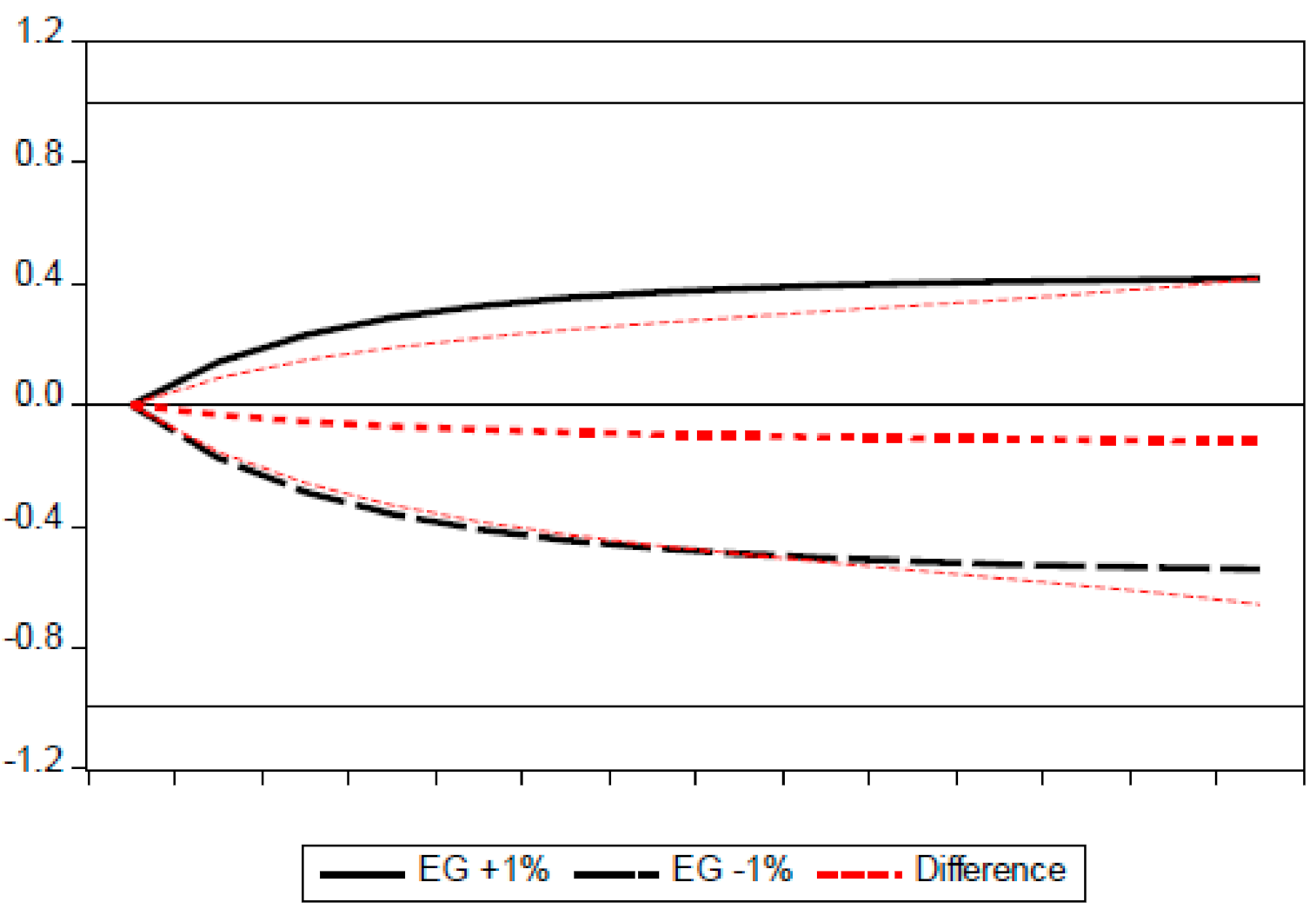
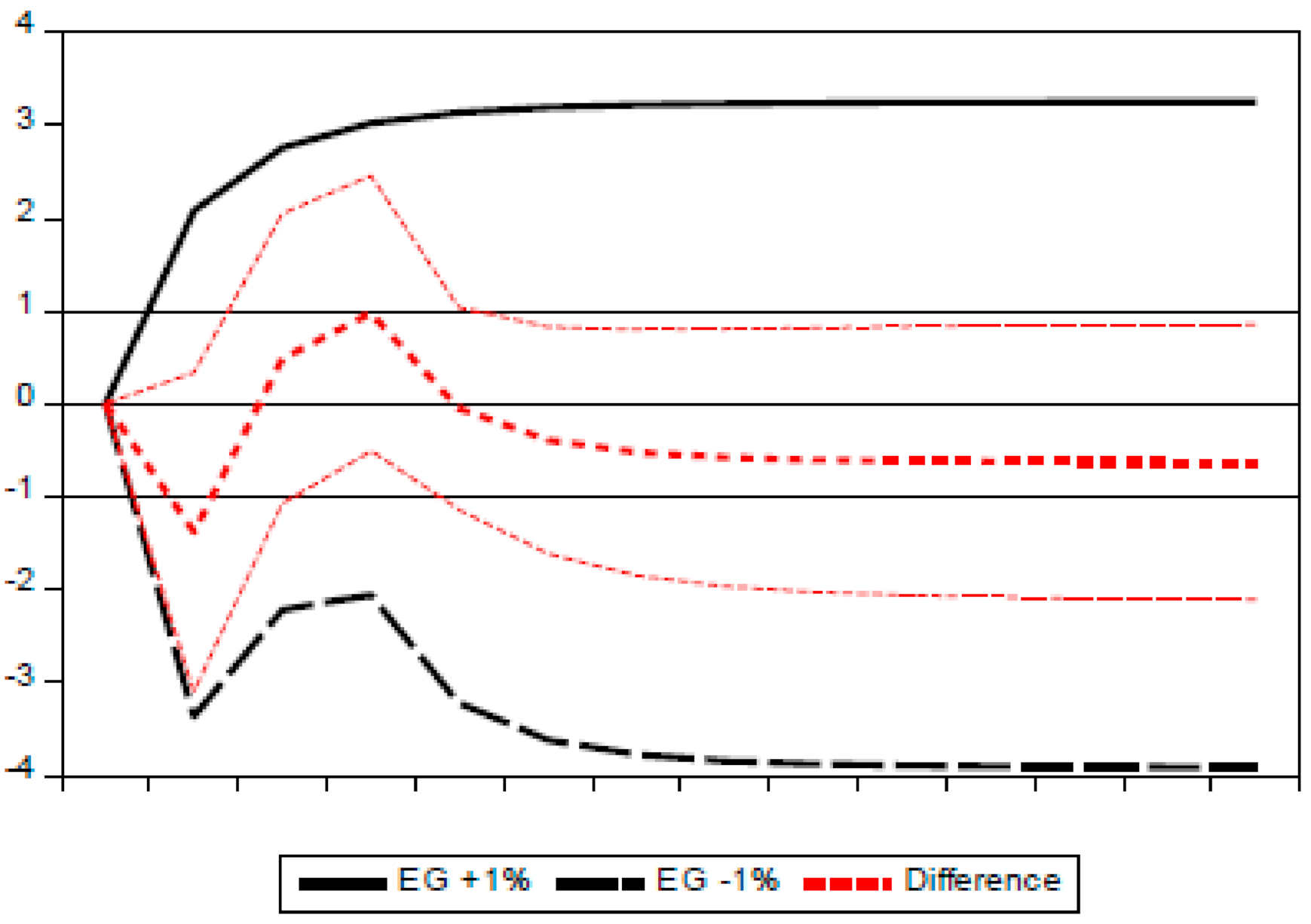
4.7. Long-Run Nonlinear Effect Results

Table 9 and Appendix A presents the projected long-run coefficients related to the negative and positive changes in energy consumption and economic growth.
Concerning the long-run link betwixt carbon emission and economic growth, a boost in Bangladesh’s economic growth leads to a negative but not statistically significant consequence on carbon emission (a coefficient −0.056) at all levels of significance. A decline in economic growth reduces carbon emission (with a coefficient of −0.379) and statistically significant. This result opposes the findings of [60], who found the existence of the conventional EKC hypothesis in Bangladesh based on bounds testing cointegration. However, the study results of [53] using the cointegration technique concluded that EKC does not exist in Venezuela, which is consistent with our findings with regards to Bangladesh. In the case of energy consumption, an increase in energy consumption not only has a positive but statistically significant effect on carbon emission (a coefficient of 0.604). However, a decrease in energy consumption has a negative and statically significant consequence (a coefficient of −0.964) on carbon emission in Bangladesh. It means that an upsurge in Bangladesh’s energy consumption contributes to a significant increase in carbon emission by 0.604%. In comparison, a down string in energy consumption will significantly cause a decline in carbon emission by 0.964%. This outcome is consistent with [97] findings of an upsurge in the consumption of energy, which contributed to environmental pollution when the author examined the relationship between energy use and economic growth employing panel estimation systems in sub-Sahara African countries.
Concerning Iran, a boom in economic growth has a negative relationship with carbon emission (a coefficient of −3.579) but statistically insignificant. While a decrease in economic growth also negatively affects carbon emissions (a coefficient of −5.924) and statistically significant. This means that a drop in economic growth will account for a 5.924% reduction in carbon emission in Iran. This outcome is also in harmony with findings from [61]. They found no presence of the EKC hypothesis when the author used time-varying Granger causality analysis to test for G7 countries. A rise in energy consumption accounts for a positive and statistically significant effect (with a coefficient of 7.161) on carbon emission. While a negative shock to energy consumption has a positive (with a coefficient of 1.493) impact on economic carbon emission but not statistically significant. Therefore, it implies that an increase in energy consumption in Iran increases carbon emission by 7.161%. This result confirms the findings of [98], who asserted that the use of energy critically affects the environment.
For Turkey, an increase in economic growth has a statistically significant positive relationship with carbon emission (a coefficient of 1.766). Additionally, a downswing in economic growth leads to a statistically significant carbon emission reduction (a coefficient of −2.555). This implies that Turkey’s economic boom increases carbon emission by 1.766%, while a decline in economic growth reduces the country’s carbon emission by 2.555%. Findings for Turkey are contrary to [51] results that found the conventional EKC hypothesis based on cointegration analysis. Moreover, the results are also in line with [17], who found out that economic growth had a compelling impact in explaining the CO2 emission in Turkey.
Nevertheless, an upsurge in energy consumption resulted in a statistically significant increase (a coefficient of 1.517) in carbon emissions. In contrast, a decrease in energy consumption led to a statistically insignificant reduction (a coefficient of −0.794) in carbon emission. In Turkey, when there was an increase in energy consumption by 1%, it led to a 1.517% rise in carbon emission in the long-run. The result of a significant increase in Turkey’s carbon emission caused by an increase in the country’s energy consumption is in line with the findings of [37,99] about the rise in carbon emissions as a result of energy consumption.
Results for Vietnam indicate that a boom in economic growth results in a statistically significant negative effect on carbon emission (a coefficient of −0.365). However, a negative shock to economic growth results in a statistically significant rise in carbon emission (a coefficient of 1.168). It implies that in Vietnam, an upsurge in economic growth lessens carbon emissions by 0.365%, while a reduction in economic growth increases carbon emissions by 1.168%. With this, an observation of the existence of the conventional EKC hypothesis is made and is contrary to findings from the works of [52,61]. Concerning energy consumption, an increase is associated with a statistically significant increase in carbon emissions (a coefficient of 1.901), while a decline in energy consumption is associated with a statistically significant reduction in carbon emissions (a coefficient of −1.665). Thus, in Vietnam, an upsurge in energy consumption consequently increased carbon emissions by 1.901%, and a reduction in energy consumption decreases carbon emissions by 1.665%. The attribution of an upsurge in carbon emissions to an upsurge in energy consumption is in line with results published from the work of [38].

4.8. Results for Nonlinear Restrictions

The Wald test results for economic growth validate the presence of long-run asymmetric effects for Bangladesh, Iran, and Vietnam. Wald test outcomes in the short-run show asymmetric effects for only Iran. We found both the long-run and the short-run asymmetric effects in Bangladesh and Iran concerning energy consumption. These results are displayed in Table 10. This asymmetric effect implies that carbon emissions reacted differently to an increase and decrease in energy consumption and economic growth in these countries.

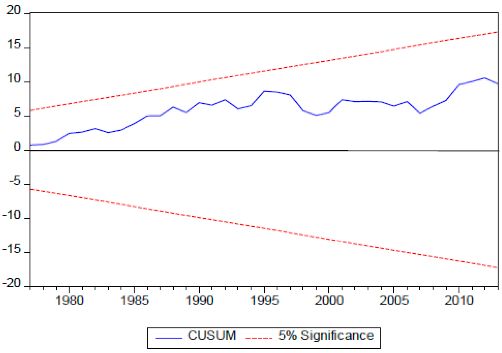
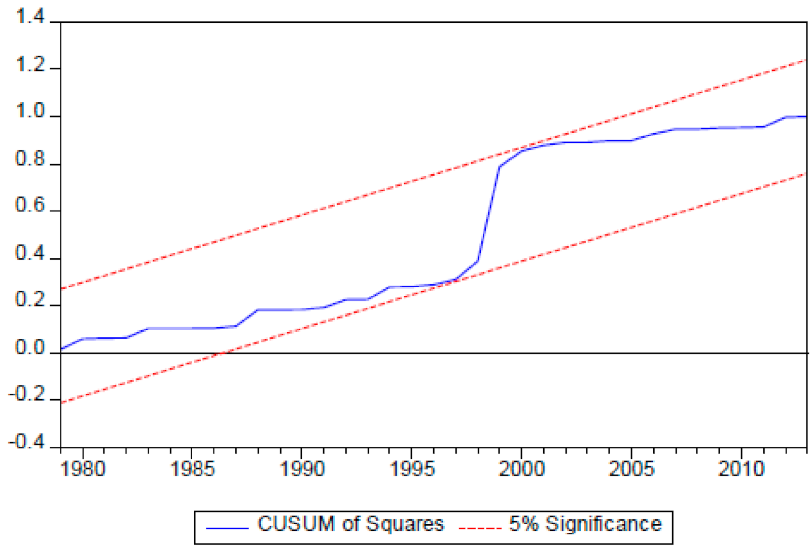
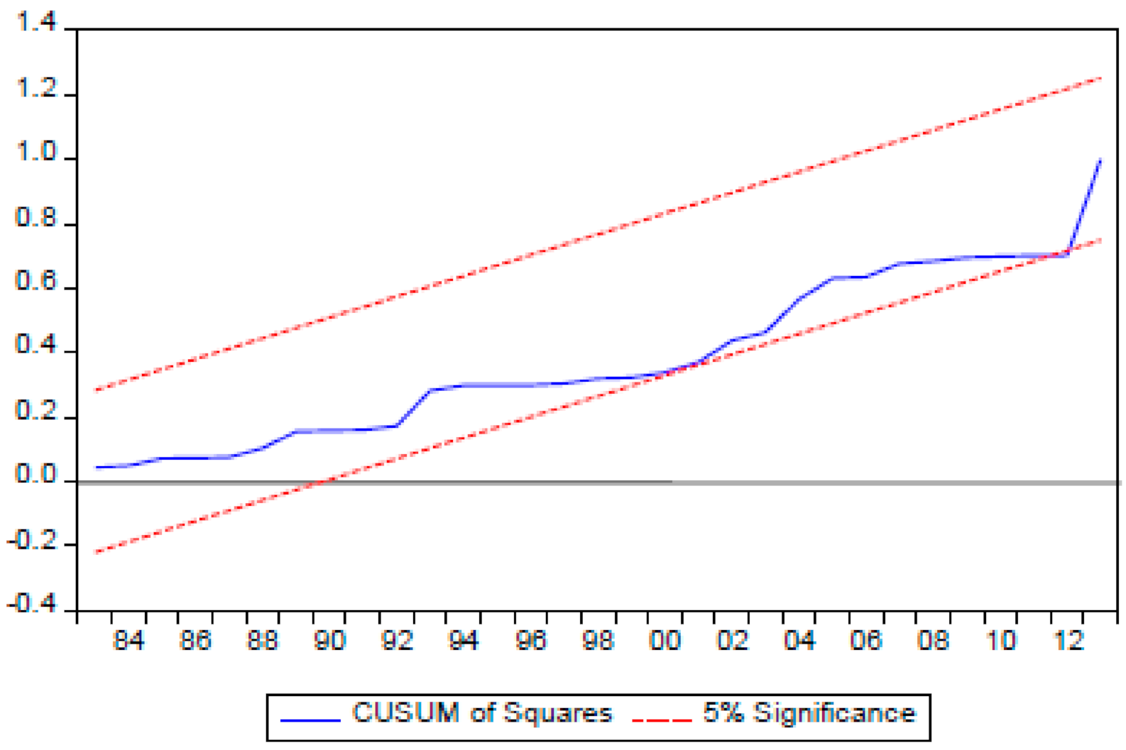
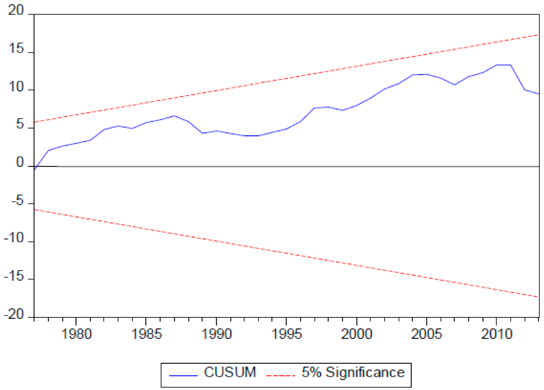
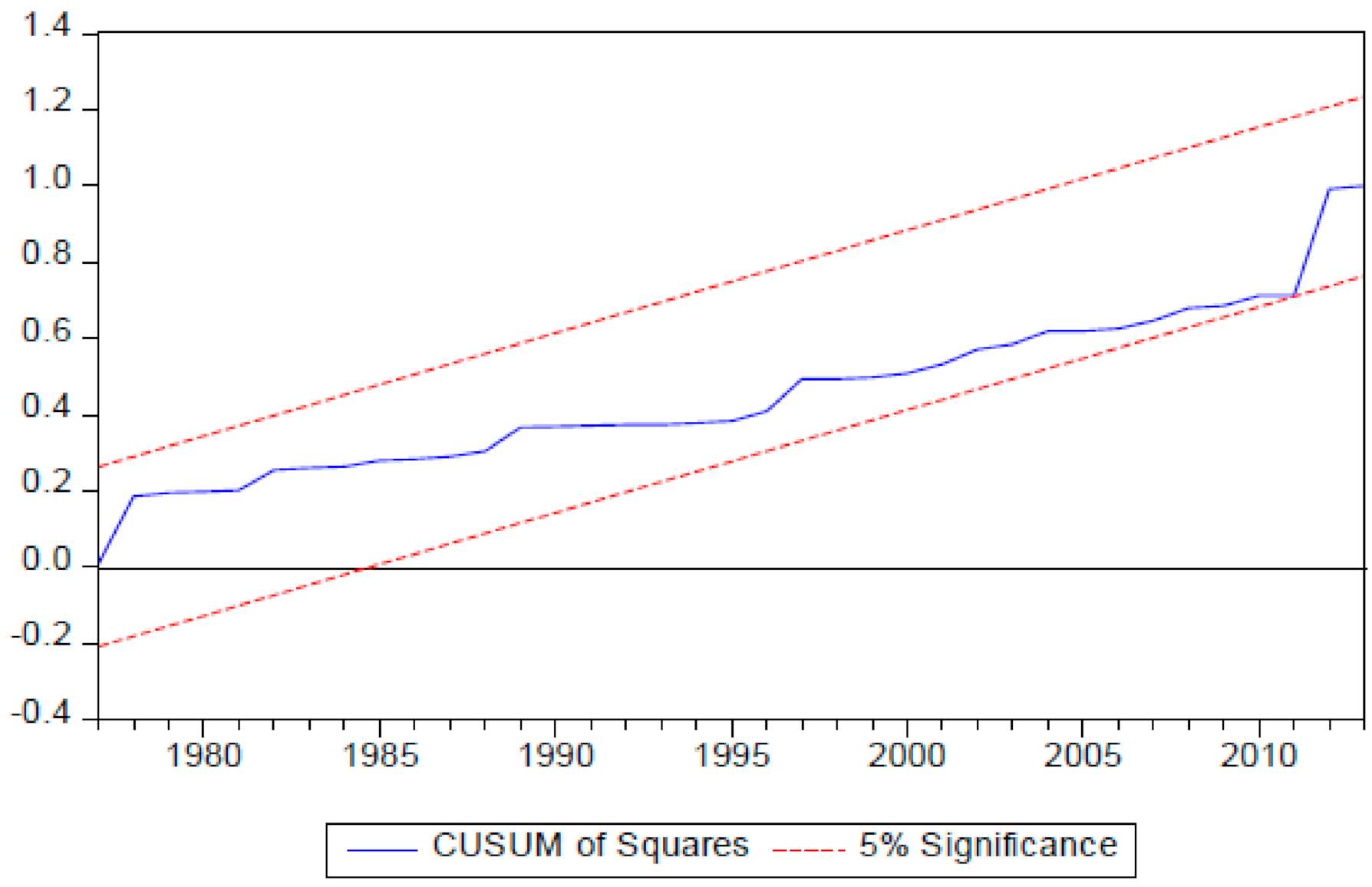
4.9. Model Stability Tests

We then present the dynamic asymmetric nexus between economic growth and carbon emissions by graphing the multipliers effects. These dynamic multipliers (see Figure 1, Figure 2, Figure 3 and Figure 4) display carbon emission adjustments to a unit change in economic growth to its new long-run equilibrium following a negative or positive single shock in the 42 years. The positive change depicted by a continuous black line and negative change indicated by dashed black line curves describes the adjustment of carbon emission to a positive and negative effect of multipliers to shocks in the 42-year economic growth at a given forecast horizon. The asymmetry line (continuous red line) indicates the variance between the negative and positive effects multipliers to shocks in the 42-year economic growth. The empirical findings affirm the presence of a nonlinear connection between carbon emission and economic growth. The occurrence of a long-run nonlinear relationship between changes in 42-year carbon emission and economic growth shows the essence to consider nonlinearity when studying the relationship among the variables.
Figure 5, Figure 6, Figure 7, Figure 8, Figure 9, Figure 10, Figure 11 and Figure 12 display the CUSUM and CUSUMSQ tests graphs. CUSUM and CUSUM of squares are utilized to explore if the coefficients are stable or not. Therefore, the two graphs validate that the model was reliable and stable since they both fell within the critical bounds at a 5% significance level.

4.10. Asymmetric Causality Results

The nonlinear Granger causality test outcomes presented in Table 11 for Bangladesh describe a feedback causality betwixt carbon emission and economic growth. It is contrary to no bidirectional causality reported from the linear Granger causality test. The outcome of [100], which is similar to ours, found a feedback causality in the long-run between carbon emission and economic growth in Bangladesh. Additionally, the unidirectional causality, which runs from energy consumption to carbon emissions as reported in the nonlinear framework, was consistent with findings presented in the linear framework in Table 5. Similar findings were made by [100] in Bangladesh and [101] in China’s case.
In Egypt, we identified a unidirectional asymmetric Granger causality connection, which runs from economic growth to carbon emission in dimension four (4) at a 10% level of statistical significance. However, it contrasts with the linear Granger causality results for Egypt but consistent with results reported by [100] in Egypt. Contrary to no causality between energy consumption and carbon emission in Egypt, we identified a nonlinear unidirectional causality that runs from energy consumption to carbon emission. Chebbi, H.E. (2010) [102] also found that energy consumption Granger causes carbon emission in Tunisia, and in South Africa, [103] made similar findings.
Our findings regarding Indonesia revealed no causality running between carbon emission and economic growth consistent with [104] in India’s study. However, [105] revealed that economic growth Granger causes carbon emission in Indonesia. Tiwari, A.K., Shahbaz, M. and Hye, Q.M.A (2013) [54] also discovered a feedback effect between carbon emission and economic growth in India. In terms of nonlinear causality, a unidirectional causality that runs from energy consumption to carbon emission is confirmed with similar findings reported in the traditional Granger causality results. Soytas, U., Sari, R. and Ewing, B.T (2007) [4] also made similar findings in the U.S. reporting that causality exists between carbon emission and energy consumption.
We discovered a unidirectional linear causality that runs from economic growth to Iran’s carbon emission. However, a unidirectional nonlinear causality was found to run from carbon emission to economic growth. No feedback causality was found between energy consumption and carbon emission in both the linear and nonlinear framework.
The nonlinear Granger causality results revealed no causality between economic growth, energy consumption, and carbon emission in Nigeria and Mexico. These results are comparable to the findings reported by [105] in the two countries using time-varying and time constant Granger causality tests.
Asymmetric causality results from Pakistan show no causality between carbon emission and economic growth, but a unidirectional causality is confirmed, running from energy consumption to carbon emission. Compared with the linear Granger causality was found running from energy consumption and economic growth to carbon emission.
In the Philippines’ economy, we found that economic growth did not Granger cause carbon emission in the symmetric framework, similar to a finding from the symmetric Granger causality results. The result is similar to [52,106] in the case of Ecuador and Venezuela, where the existence of the EKC hypothesis could not be found. However, a unidirectional causality that runs from carbon emission to energy consumption was found from the asymmetric results contrary to no causality between the variables in the symmetric results. Using a dynamic Granger causality test [103] also found that carbon emission and economic growth in the Philippines led to energy consumption.
Regarding South Korea, our results indicate a significant asymmetric Granger causality that runs from economic growth to carbon emission, which implies that economic growth causes carbon emission, which confirms the existence of the EKC hypothesis. Baek (2015) and [105] also confirmed the existence of EKC in South Korea in their studies. It is comparable to the results of symmetric Granger causality, which indicates that the economic growth Granger causes carbon emission in South Korea. Additionally, in both the linear and nonlinear causality framework, energy consumption leads to carbon emission. In a similar study, [26] also found asymmetric causality that runs from energy consumption to carbon emission in Italy and France.
In Turkey’s economy, the null hypothesis of no asymmetric Granger causality that runs from economic growth to carbon emission and vice versa was rejected. It means that an asymmetric Granger causality relation exists from carbon emission to economic growth vice versa. This finding is divergent to results reported in the linear Granger causality structure, signifying no bidirectional causality between the variables in Turkey. However, the asymmetric causality results are similar to findings made by [51] in Turkey, where they affirmed the existence of the EKC hypothesis. We identified a unidirectional asymmetric causality that runs from carbon emission to energy consumption whiles no linear causality was reported. Lean, H.H. and Smyth, R (2010) [107] also reported a causal relationship that runs from electricity consumption to carbon emission in Asian Nations.
Asymmetric Granger causality results from Vietnam also show no feedback causality betwixt carbon emission and economic growth in contrast to bidirectional linear Granger causality result reported earlier. However, linear Granger causality outcomes reported earlier shows a unidirectional causality from economic growth to carbon emission in the case of Vietnam. The asymmetric Granger causality results are in contrast with findings made by [105], who also found a linear relationship from economic growth to carbon emission in Vietnam. However, it is consistent with [52,61]. We found bidirectional asymmetric causality between energy consumption and carbon emission consistent with [60] in the case of Bangladesh.

5. Conclusions and Recommendations

This research contributes to the significant debate on the nexus between carbon emission, energy consumption, and economic growth. Our analysis was based on the 42 years (1972–2013) data on carbon emission, energy consumption, and economic growth for the next 11 (N-11) countries globally. Nonlinear A.R.D.L. and linear Granger causality tests were applied to investigate the cointegration and causality link among the variables. The empirical findings show a significant rejection of a significant feedback causality connection between the dependent variable (carbon emission) and the two independent variables (economic growth and energy consumption) in all of the N11 countries excluding Vietnam. Vietnam shows a bidirectional Granger causality betwixt carbon emission and energy consumption and unidirectional causality that runs from economic growth to carbon emission. Economic growth granger causing carbon emissions were observed in South Korea, Bangladesh, Mexico, Iran, Indonesia, and Pakistan.
Meanwhile, in Egypt, a unidirectional causality nexus running from carbon emission to economic growth was observed. Furthermore, Indonesia, Pakistan, and South Korea displayed a unidirectional Granger causality running from energy consumption to carbon emission. Interestingly, no Granger causality relationship was found to exist between carbon emission, energy consumption, and economic growth in both Nigeria and Turkey.
Various vital findings were attained from the N.A.R.D.L. bounds testing analysis outcomes. The nonlinear cointegration outcomes show four significant long-run links between economic growth, carbon emissions, and energy consumption at usual significance levels for Bangladesh, Iran, Turkey, and Vietnam. Substantial evidence was also obtained from our long-run asymmetric effect results. Concerning the linkage between economic growth and carbon emission, we obtained evidence that showed the EKC hypothesis exists in Vietnam but does not exist in Bangladesh, Iran, and Turkey. For Bangladesh and Iran, an upsurge in economic growth has a statistically insignificant negative consequence on carbon emission, while a decrease in economic growth has a statistically significant negative consequence on carbon emissions.
On the other hand, results for Vietnam show that a boost to economic development leads to a statistically significant negative consequence on carbon emission, confirming the EKC hypothesis. In contrast, a reduction in economic growth results in a statistically significant upsurge in carbon emissions. No evidence of the existence of the EKC hypothesis was established for Turkey because an expansion in economic growth has a statistically significant positive relationship with carbon emission. In contrast, a downswing in economic growth leads to a statistically significant reduction in carbon emissions. Concerning the EKC hypothesis, the mixed results obtained were consistent with findings from [56,58]. In the case of the relationship between carbon emission and energy consumption, we found evidence of a positive shock to energy consumption, leading to a statistically significant increase in carbon emissions in Bangladesh, Iran, Turkey, and Vietnam. In contrast, a negative shock in energy consumption leads to a statistically significant decrease in carbon emissions in Bangladesh and Vietnam. Moreover, negative shocks in energy consumption for Iran and Turkey both obtained statistically insignificant effects, with Iran and Turkey having a statistically insignificant increase in carbon emissions and a statistically insignificant decrease in carbon emissions, respectively.
According to the Wald test results, with regards to nonlinear associations, long-run results show evidence of an asymmetric relationship between carbon emissions and economic growth in Bangladesh, Iran, and Vietnam. For carbon consumption and energy emission, long-run asymmetries were found in Bangladesh and Iran. Short-run asymmetries between carbon emissions and energy consumption were observed for both Bangladesh and Iran. In contrast, short-run asymmetries between carbon emissions and economic growth were only observed for Iran.
Based on these findings, Bangladeshi policymakers can tackle the problem of carbon emissions by controlling energy consumption. From our analysis, changes in economic growth do not have a significant increasing influence on carbon emissions. Instead, changes in energy consumption have huge impacts on carbon emissions. Hence, new alternative sources of energy must be explored by Bangladesh’s government by implementing energy exploring policies and investing in renewable energy systems, which will help reduce cumulative amounts of carbon emissions without affecting its economic growth.
Iranian policymakers should also focus on the energy consumption of the country. From our analysis, a decline in economic growth significantly reduces Iran’s carbon emission, but this will not be the path the Iranian government would want to pursue. Thus, without affecting the country’s economic growth, the Iranian government can also explore new energy sources and switch to renewable energy to reduce carbon emissions. Expediently, the government can encourage both local and foreign investors to adopt energy sufficient technologies without reducing their productivity level.
Economic growth can play a significant role in reducing energy consumption; consequently, it has an insignificant effect on carbon emissions. The Turkish government should improve its environmental quality by introducing carbon emission trading and tax schemes. The government can also initiate educational programs about the dangers associated with carbon emissions to help create awareness. The government should make sure that those responsible do implement these recommended policies, and those who fail to adhere should face the full force of the law. Policymakers in Turkey can also embrace forceful investment in developing energy expertise and elevating energy exploration to accomplish technological breakthroughs that will possibly empower the nation to deliver more output with lesser emissions. Investment can also be made into green energy technologies such as e-transport. The usage of e-bikes, e-cars, e-trains, and e-buses like what is being implemented in China can go a long way to help drastically reduce the carbon emissions in Turkey.
Interestingly, findings for Vietnam enable the issue of carbon emissions to be tackled from both the economic growth aspect and the energy consumption aspect. From our results for Vietnam, a boost in economic growth reduced carbon emissions significantly, and a reduction in economic growth boosts the carbon emissions. With the expansion of the Vietnamese economy, carbon emissions reduced significantly. Policymakers have put in place tight regulations to lessen the level of carbon emissions of the country. Additionally, the adoption of improved technological equipment and investment into renewable energy has helped the country decrease carbon emissions level without affecting its economic growth. The Vietnamese government can still explore new energy sources from the energy consumption aspect by investing in other untapped renewable energy available.
Finally, empirical results from the entire sample of the next 11 countries indicate a significant increase in carbon emission linked to economic growth. A corresponding increase in energy consumption in some countries should be a global concern. Therefore market-based policy options such as “polluter pay”, which require the imposition of fees and taxes such as carbon taxes on industries associated with high carbon emissions in their operations. Additionally, public policies aimed at moving to the use of environmentally friendly energy production projects should be aggressively rolled out and implemented.

Author Contributions

Conceptualization, G.K.M.A.; methodology, G.K.M.A.; validation, J.C., E.T.A. and D.A.A.; formal analysis, G.K.M.A. and E.T.A.; data curation, E.T.A.; writing—original draft preparation, D.A.A. and E.T.A.; writing—review and editing, G.K.M.A.; supervision, J.C.; funding acquisition, J.C. All authors have read and agreed to the published version of the manuscript.

Funding

This research was supported by the Major Project Topic of the National Natural Science Foundation “Research on the Supply, Security and Management Policy of Strategic Key Mineral Resources in the New Era” (Grant No. 71991482).

Institutional Review Board Statement

Not applicable.

Informed Consent Statement

Not applicable.

Data Availability Statement

Not applicable.

Conflicts of Interest

The authors declare no conflict of interest.

Appendix A

Table A1. Summary of the long-run asymmetric effects of economic growth and energy consumption on carbon emission.
CountriesPositive and Negative Changes in Economic Growth and Energy Consumption (Independent Variables)The outcome of Changes in Independent Variables (Economic Growth and Energy Consumption) on the Dependent Variable (Carbon Emission)
BangladeshIncrease in economic growthReduces carbon emission but not significant
A decrease in economic growthA significant decline in carbon emission
Increase in energy consumptionSignificantly increases carbon emission
A decrease in energy consumptionLeads to a significant reduction in carbon emission
IranIncrease in economic growthDecreases carbon emission but not significant
A decrease in economic growthCarbon emission decreases significantly
Increase in energy consumption A significant rise in carbon emissions
A decrease in energy consumptionCarbon emission increases but not significant
TurkeyIncrease in economic growthA significant upsurge in carbon emissions
A decrease in economic growthCarbon emission declines significantly
Increase in energy consumptionA significant rise in carbon emission
A decrease in energy consumptionA nonsignificant reduction in carbon emissions
VietnamIncrease in economic growthSignificantly decreases carbon emission
A decrease in economic growthIncreases carbon emissions significantly
Increase in energy consumptionCarbon emissions significantly rise
A decrease in energy consumptionA significant decline in carbon emissions

References

  1. Owusu, P.A.; Asumadu-Sarkodie, S. A review of renewable energy sources, sustainability issues and climate change mitigation. Cogent Eng. 2016, 3, 1167990. [Google Scholar] [CrossRef]
  2. The World Bank. The World Bank Annual Report 2007; The World Bank: Washington, DC, USA, 2007. [Google Scholar]
  3. Perry, L.G.; Andersen, D.C.; Reynolds, L.V.; Nelson, S.M.; Shafroth, P.B. Vulnerability of riparian ecosystems to elevated CO 2 and climate change in arid and semiarid western N orth A merica. Glob. Chang. Biol. 2011, 18, 821–842. [Google Scholar] [CrossRef]
  4. Soytas, U.; Sari, R.; Ewing, B.T. Energy consumption, income, and carbon emissions in the United States. Ecol. Econ. 2007, 62, 482–489. [Google Scholar] [CrossRef]
  5. Bello, M.O.; Solarin, S.A.; Yen, Y.Y. The impact of electricity consumption on CO2 emission, carbon footprint, water footprint and ecological footprint: The role of hydropower in an emerging economy. J. Environ. Manag. 2018, 219, 218–230. [Google Scholar] [CrossRef] [PubMed]
  6. Stern, F. Electron Exchange Energy in Si Inversion Layers. Phys. Rev. Lett. 1973, 30, 278–280. [Google Scholar] [CrossRef]
  7. Stern, D.I. Energy and economic growth in the USA: A multivariate approach. Energy Econ. 1993, 15, 137–150. [Google Scholar] [CrossRef]
  8. Solomon, S. IPCC (2007): Climate change the physical science basis. AGUFM 2007, 2007, U43D-01. [Google Scholar]
  9. Sarkodie, S.A.; Adams, S. Renewable energy, nuclear energy, and environmental pollution: Accounting for political institutional quality in South Africa. Sci. Total. Environ. 2018, 643, 1590–1601. [Google Scholar] [CrossRef]
  10. Apergis, N.; Jebli, M.B.; Youssef, S.B. Does renewable energy consumption and health expenditures decrease carbon dioxide emissions? Evidence for sub-Saharan Africa countries. Renew. Energy 2018, 127, 1011–1016. [Google Scholar] [CrossRef]
  11. Ang, J.B. Economic development, pollutant emissions and energy consumption in Malaysia. J. Policy Model. 2008, 30, 271–278. [Google Scholar] [CrossRef]
  12. Omri, A. CO2 emissions, energy consumption and economic growth nexus in MENA countries: Evidence from simultaneous equations models. Energy Econ. 2013, 40, 657–664. [Google Scholar] [CrossRef] [Green Version]
  13. Hanif, I. Impact of economic growth, nonrenewable and renewable energy consumption, and urbanization on carbon emissions in Sub-Saharan Africa. Environ. Sci. Pollut. Res. 2018, 25, 15057–15067. [Google Scholar] [CrossRef] [PubMed]
  14. Brandt, A.R. How does energy resource depletion affect prosperity? Mathematics of a minimum energy return on investment (EROI). Biophys. Econ. Resour. Qual. 2017, 2, 1986. [Google Scholar] [CrossRef] [Green Version]
  15. Eggleston, H.S.; Buendia, L.; Miwa, K.; Ngara, T.; Tanabe, K. 2006 IPCC Guidelines for National Greenhouse Gas Inventories; Institute for Global Environmental Strategies: Hayama, Japan, 2006; Volume 5. [Google Scholar]
  16. International Energy Agency. World Energy Outlook 2011; International Energy Agency: Paris, France, 2011; p. 666. [Google Scholar]
  17. Halicioglu, F. An econometric study of CO2 emissions, energy consumption, income and foreign trade in Turkey. Energy Policy 2009, 37, 1156–1164. [Google Scholar] [CrossRef] [Green Version]
  18. Ozturk, I.; Acaravci, A. CO2 emissions, energy consumption and economic growth in Turkey. Renew. Sustain. Energy Rev. 2010, 14, 3220–3225. [Google Scholar] [CrossRef]
  19. Tamazian, A.; Chousa, J.P.; Vadlamannati, K.C. Does higher economic and financial development lead to environmental degradation: Evidence from BRIC countries. Energy Policy 2009, 37, 246–253. [Google Scholar] [CrossRef]
  20. Adamantiades, A.; Kessides, I.N. Nuclear power for sustainable development: Current status and future prospects. Energy Policy 2009, 37, 5149–5166. [Google Scholar] [CrossRef]
  21. DeCanio, S.J. The political economy of global carbon emissions reductions. Ecol. Econ. 2009, 68, 915–924. [Google Scholar] [CrossRef]
  22. Reddy, B.S.; Assenza, G.B. The great climate debate. Energy Policy 2009, 37, 2997–3008. [Google Scholar] [CrossRef]
  23. Sachs, G. The future of finance, The rise of the new Shadow Bank, New York. Goldman Sachs Equity Res. 2015, 3. Available online: https://www.fdic.gov/analysis/cfr/bank-research-conference/annual-17th/papers/15-piskorski.pdf (accessed on 18 January 2021).
  24. The World Bank. World Development Report 2015: Mind, Society, and Behavior; The World Bank: Washington, DC, USA, 2015. [Google Scholar]
  25. US Energy Information Administration. Electric Power Annual 2012; US Energy Information Administration: Washington, DC, USA, 2015.
  26. Bosah, P.; Li, S.; Ampofo, G.K.M.; Asante, D.A.; Wang, Z. The Nexus Between Electricity Consumption, Economic Growth, and CO2 Emission: An Asymmetric Analysis Using Nonlinear ARDL and Nonparametric Causality Approach. Energies 2020, 13, 1258. [Google Scholar] [CrossRef] [Green Version]
  27. Raggad, B. Economic development, energy consumption, financial development, and carbon dioxide emissions in Saudi Arabia: New evidence from a nonlinear and asymmetric analysis. Environ. Sci. Pollut. Res. 2020, 27, 21872–21891. [Google Scholar] [CrossRef] [PubMed]
  28. Shin, Y.; Yu, B.; Greenwood-Nimmo, M. Modelling asymmetric cointegration and dynamic multipliers in a nonlinear ARDL framework. In Festschrift in Honor of Peter Schmidt; Springer Science & Business Media: New York, NY, USA, 2014; pp. 281–314. [Google Scholar]
  29. Diks, C.; Panchenko, V. A new statistic and practical guidelines for nonparametric Granger causality testing. J. Econ. Dyn. Control 2006, 30, 1647–1669. [Google Scholar] [CrossRef] [Green Version]
  30. Hiemstra, C.; Jones, J.D. Testing for linear and nonlinear Granger causality in the stock price-volume relation. J. Financ. 1994, 49, 1639–1664. [Google Scholar]
  31. GrossmanGM, K. Environmental Impacts of the North American Free Trade Agreement; NBER: Cambridge, UK, 1991. [Google Scholar]
  32. Kuznets, S. Economic growth and income inequality. Am. Econ. Rev. 1955, 45, 1–28. [Google Scholar]
  33. Ahmad, A.; Zhao, Y.; Shahbaz, M.; Bano, S.; Zhang, Z.; Wang, S.; Liu, Y. Carbon emissions, energy consumption and economic growth: An aggregate and disaggregate analysis of the Indian economy. Energy Policy 2016, 96, 131–143. [Google Scholar] [CrossRef]
  34. Gao, J.; Zhang, L. Electricity Consumption–Economic Growth—CO2 Emissions Nexus in Sub-Saharan Africa: Evidence from Panel Cointegration. Afr. Dev. Rev. 2014, 26, 359–371. [Google Scholar] [CrossRef]
  35. Bargaoui, Z.K.; Chebbi, A. Comparison of two kriging interpolation methods applied to spatiotemporal rainfall. J. Hydrol. 2009, 365, 56–73. [Google Scholar] [CrossRef]
  36. Al-Mulali, U.; Solarin, S.A.; Ozturk, I. Investigating the presence of the environmental Kuznets curve (EKC) hypothesis in Kenya: An autoregressive distributed lag (ARDL) approach. Nat. Hazards 2016, 80, 1729–1747. [Google Scholar] [CrossRef]
  37. Menyah, K.; Wolde-Rufael, Y. CO2 emissions, nuclear energy, renewable energy and economic growth in the US. Energy Policy 2010, 38, 2911–2915. [Google Scholar] [CrossRef]
  38. Hamit-Haggar, M. Greenhouse gas emissions, energy consumption and economic growth: A panel cointegration analysis from Canadian industrial sector perspective. Energy Econ. 2012, 34, 358–364. [Google Scholar] [CrossRef]
  39. Pao, H.-T.; Tsai, C.-M. Multivariate Granger causality between CO2 emissions, energy consumption, FDI (foreign direct investment) and GDP (gross domestic product): Evidence from a panel of BRIC (Brazil, Russian Federation, India, and China) countries. Energy 2011, 36, 685–693. [Google Scholar] [CrossRef]
  40. Pao, H.-T.; Tsai, C.-M. CO2 emissions, energy consumption and economic growth in BRIC countries. Energy Policy 2010, 38, 7850–7860. [Google Scholar] [CrossRef]
  41. Mendum, R.; Njenga, M. Integrating wood fuels into agriculture and food security agendas and research in sub-Saharan Africa. Facets 2018, 3, 1–11. [Google Scholar] [CrossRef] [Green Version]
  42. Lorde, T.; Waithe, K.; Francis, B. The importance of electrical energy for economic growth in Barbados. Energy Econ. 2010, 32, 1411–1420. [Google Scholar] [CrossRef]
  43. Mezghani, I.; Haddad, H.B. Energy consumption and economic growth: An empirical study of the electricity consumption in Saudi Arabia. Renew. Sustain. Energy Rev. 2017, 75, 145–156. [Google Scholar] [CrossRef]
  44. Paramati, S.R.; Sinha, A.; Dogan, E. The significance of renewable energy use for economic output and environmental protection: Evidence from the Next 11 developing economies. Environ. Sci. Pollut. Res. 2017, 24, 13546–13560. [Google Scholar] [CrossRef]
  45. Solarin, S.A.; Lean, H.H. Natural gas consumption, income, urbanization, and CO2 emissions in China and India. Environ. Sci. Pollut. Res. 2016, 23, 18753–18765. [Google Scholar] [CrossRef]
  46. Esteve, V.; Tamarit, C. Threshold cointegration and nonlinear adjustment between CO2 and income: The environmental Kuznets curve in Spain, 1857–2007. Energy Econ. 2012, 34, 2148–2156. [Google Scholar] [CrossRef]
  47. Esteve, V.; Tamarit, C. Is there an environmental Kuznets curve for Spain? Fresh evidence from old data. Econ. Model. 2012, 29, 2696–2703. [Google Scholar] [CrossRef]
  48. Fosten, J.; Morley, B.; Taylor, T. Dynamic misspecification in the environmental Kuznets curve: Evidence from CO2 and SO2 emissions in the United Kingdom. Ecol. Econ. 2012, 76, 25–33. [Google Scholar] [CrossRef] [Green Version]
  49. Shahbaz, M.; Lean, H.H.; Shabbir, M.S. Environmental Kuznets curve hypothesis in Pakistan: Cointegration and Granger causality. Renew. Sustain. Energy Rev. 2012, 16, 2947–2953. [Google Scholar] [CrossRef] [Green Version]
  50. Shahbaz, M.; Mutascu, M.; Azim, P. Environmental Kuznets curve in Romania and the role of energy consumption. Renew. Sustain. Energy Rev. 2013, 18, 165–173. [Google Scholar] [CrossRef] [Green Version]
  51. Shahbaz, M.; Ozturk, I.; Afza, T.; Ali, A. Revisiting the environmental Kuznets curve in a global economy. Renew. Sustain. Energy Rev. 2013, 25, 494–502. [Google Scholar] [CrossRef] [Green Version]
  52. Robalino-López, A.; Nieto, A.I.M.; García-Ramos, J.-E.; Golpe, A.A. Studying the relationship between economic growth, CO2 emissions, and the environmental Kuznets curve in Venezuela (1980–2025). Renew. Sustain. Energy Rev. 2015, 41, 602–614. [Google Scholar] [CrossRef] [Green Version]
  53. Sephton, P.; Mann, J. Further evidence of an environmental Kuznets curve in Spain. Energy Econ. 2013, 36, 177–181. [Google Scholar] [CrossRef]
  54. Tiwari, A.K.; Shahbaz, M.; Hye, Q.M.A. The environmental Kuznets curve and the role of coal consumption in India: Cointegration and causality analysis in an open economy. Renew. Sustain. Energy Rev. 2013, 18, 519–527. [Google Scholar] [CrossRef] [Green Version]
  55. Cicea, C.; Marinescu, C.; Popa, I.; Dobrin, C. Environmental efficiency of investments in renewable energy: Comparative analysis at macroeconomic level. Renew. Sustain. Energy Rev. 2014, 30, 555–564. [Google Scholar] [CrossRef]
  56. Cowan, W.N.; Chang, T.; Inglesi-Lotz, R.; Gupta, R. The nexus of electricity consumption, economic growth and CO2 emissions in the BRICS countries. Energy Policy 2014, 66, 359–368. [Google Scholar] [CrossRef] [Green Version]
  57. Ibrahim, M.H.; Law, S.H. Social capital and CO2 emission—output relations: A panel analysis. Renew. Sustain. Energy Rev. 2014, 29, 528–534. [Google Scholar] [CrossRef]
  58. Robalino-López, A.; Mena-Nieto, A.; García-Ramos, J.E. System dynamics modeling for renewable energy and CO2 emissions: A case study of Ecuador. Energy Sustain. Dev. 2014, 20, 11–20. [Google Scholar] [CrossRef] [Green Version]
  59. Shahbaz, M.; Khraief, N.; Uddin, G.S.; Ozturk, I. Environmental Kuznets curve in an open economy: A bounds testing and causality analysis for Tunisia. Renew. Sustain. Energy Rev. 2014, 34, 325–336. [Google Scholar] [CrossRef] [Green Version]
  60. Shahbaz, M.; Uddin, G.S.; Rehman, I.U.; Imran, K. Industrialization, electricity consumption and CO2 emissions in Bangladesh. Renew. Sustain. Energy Rev. 2014, 31, 575–586. [Google Scholar] [CrossRef]
  61. Ajmi, A.N.; Hammoudeh, S.; Nguyen, D.K.; Sato, J.R. On the relationships between CO2 emissions, energy consumption and income: The importance of time variation. Energy Econ. 2015, 49, 629–638. [Google Scholar] [CrossRef]
  62. Baek, J. A panel cointegration analysis of CO2 emissions, nuclear energy and income in major nuclear generating countries. Appl. Energy 2015, 145, 133–138. [Google Scholar] [CrossRef]
  63. Ramadan El, A.M.; Kamel, M.M. The Relationship Between Economic Growth and Environmental Pollution: Testing The Environmental Kuznets Curve Hypothesis in Egypt. Available online: https://www.researchgate.net/profile/Maie_Kamel/publication/336563247_The_Environmental_Kuznets_Curve_Hypothesis_in_Egypt/links/5da5c2f492851caa1ba600fa/The-Environmental-Kuznets-Curve-Hypothesis-in-Egypt.pdf (accessed on 18 January 2021).
  64. Zhang, X.; Zhang, H.; Yuan, J. Economic growth, energy consumption, and carbon emission nexus: Fresh evidence from developing countries. Environ. Sci. Pollut. Res. 2019, 26, 26367–26380. [Google Scholar] [CrossRef]
  65. Aydoğan, B.; Vardar, G. Evaluating the role of renewable energy, economic growth and agriculture on CO2 emission in E7 countries. Int. J. Sustain. Energy 2020, 39, 335–348. [Google Scholar] [CrossRef]
  66. Demissew Beyene, S.; Kotosz, B. Testing the environmental Kuznets curve hypothesis: An empirical study for East African countries. Int. J. Environ. Stud. 2020, 77, 636–654. [Google Scholar] [CrossRef] [Green Version]
  67. Destek, M.A.; Shahbaz, M.; Okumus, I.; Hammoudeh, S.; Sinha, A. The relationship between economic growth and carbon emissions in G-7 countries: Evidence from time-varying parameters with a long history. Environ. Sci. Pollut. Res. 2020, 27, 29100–29117. [Google Scholar] [CrossRef]
  68. Jin, T.; Kim, J. Investigating the environmental Kuznets curve for Annex I countries using heterogeneous panel data analysis. Environ. Sci. Pollut. Res. 2020, 27, 10039–10054. [Google Scholar] [CrossRef]
  69. Ongan, S.; Işık, C.; Ozdemir, D. Economic growth and environmental degradation: Evidence from the US case environmental Kuznets curve hypothesis with application of decomposition. J. Environ. Econ. Policy 2020. [Google Scholar] [CrossRef]
  70. Isik, C.; Ongan, S.; Özdemir, D. The economic growth/development and environmental degradation: Evidence from the US state-level EKC hypothesis. Environ. Sci. Pollut. Res. 2019, 26, 30772–30781. [Google Scholar] [CrossRef] [PubMed]
  71. Jebli, M.B.; Kahia, M. The interdependence between CO2 emissions, economic growth, renewable and nonrenewable energies, and service development: Evidence from 65 countries. Clim. Chang. 2020, 162, 193–212. [Google Scholar] [CrossRef]
  72. Erdogan, S.; Okumus, I.; Guzel, A.E. Revisiting the Environmental Kuznets Curve hypothesis in OECD countries: The role of renewable, nonrenewable energy, and oil prices. Environ. Sci. Pollut. Res. 2020, 1–9, 23655–23663. [Google Scholar] [CrossRef]
  73. Kotroni, E.; Kaika, D.; Zervas, E. Environmental Kuznets Curve in Greece in the period 1960–2014. Int. J. Energy Econ. Policy 2020, 10, 364–370. [Google Scholar] [CrossRef]
  74. Koc, S.; Bulus, G.C. Testing validity of the EKC hypothesis in South Korea: Role of renewable energy and trade openness. Environ. Sci. Pollut. Res. 2020, 27, 29043–29054. [Google Scholar] [CrossRef]
  75. Mrabet, Z.; AlSamara, M.; Jarallah, S.H. The impact of economic development on environmental degradation in Qatar. Environ. Ecol. Stat. 2017, 24, 7–38. [Google Scholar] [CrossRef]
  76. Jalil, A.; Feridun, M. The impact of growth, energy and financial development on the environment in China: A cointegration analysis. Energy Econ. 2011, 33, 284–291. [Google Scholar] [CrossRef]
  77. Onafowora, O.A.; Owoye, O. Bounds testing approach to analysis of the environment Kuznets curve hypothesis. Energy Econ. 2014, 44, 47–62. [Google Scholar] [CrossRef]
  78. Ozturk, I.; Acaravci, A. The long-run and causal analysis of energy, growth, openness and financial development on carbon emissions in Turkey. Energy Econ. 2013, 36, 262–267. [Google Scholar] [CrossRef]
  79. Shahbaz, M.; Nasreen, S.; Ahmed, K.; Hammoudeh, S. Trade openness–carbon emissions nexus: The importance of turning points of trade openness for country panels. Energy Econ. 2017, 61, 221–232. [Google Scholar] [CrossRef] [Green Version]
  80. Boutabba, M.A. The impact of financial development, income, energy and trade on carbon emissions: Evidence from the Indian economy. Econ. Model. 2014, 40, 33–41. [Google Scholar] [CrossRef] [Green Version]
  81. Shahzad, S.J.H.; Kumar, R.R.; Zakaria, M.; Hurr, M. Carbon emission, energy consumption, trade openness and financial development in Pakistan: A revisit. Renew. Sustain. Energy Rev. 2017, 70, 185–192. [Google Scholar] [CrossRef]
  82. Shahbaz, M.; Solarin, S.A.; Mahmood, H.; Arouri, M. Does financial development reduce CO2 emissions in Malaysian economy? A time series analysis. Econ. Model. 2013, 35, 145–152. [Google Scholar] [CrossRef] [Green Version]
  83. Yeh, J.-C.; Liao, C.-H. Impact of population and economic growth on carbon emissions in Taiwan using an analytic tool stirpat. Sustain. Environ. Res. 2017, 27, 41–48. [Google Scholar] [CrossRef] [Green Version]
  84. Shi, A. Population growth and global carbon dioxide emissions. In Proceedings of the IUSSP Conference in Brazil/SESSION-S09. 2001. Available online: https://iussp.org/sites/default/files/Brazil2001/s00/S09_04_Shi.pdf (accessed on 18 January 2021).
  85. Shahbaz, M.; Mallick, H.; Mahalik, M.K.; Loganathan, N. Does globalization impede environmental quality in India? Ecol. Indic. 2015, 52, 379–393. [Google Scholar] [CrossRef] [Green Version]
  86. Baz, K.; Xu, D.; Ali, H.; Ali, I.; Khan, I.; Khan, M.M.; Cheng, J. Asymmetric impact of energy consumption and economic growth on ecological footprint: Using asymmetric and nonlinear approach. Sci. Total Environ. 2020, 718, 137364. [Google Scholar] [CrossRef]
  87. Javid, M.; Sharif, F. Environmental Kuznets curve and financial development in Pakistan. Renew. Sustain. Energy Rev. 2016, 54, 406–414. [Google Scholar] [CrossRef]
  88. Abbasi, F.; Riaz, K. CO2 emissions and financial development in an emerging economy: An augmented VAR approach. Energy Policy 2016, 90, 102–114. [Google Scholar] [CrossRef]
  89. Hang, G.; Yuan-Sheng, J. The relationship between CO2 emissions, economic scale, technology, income and population in China. Procedia Environ. Sci. 2011, 11, 1183–1188. [Google Scholar] [CrossRef] [Green Version]
  90. Mardani, A.; Streimikiene, D.; Nilashi, M.; Arias-Aranda, D.; Loganathan, N.; Jusoh, A. Energy consumption, economic growth, and CO2 emissions in G20 countries: Application of adaptive neuro-fuzzy inference System. Energies 2018, 11, 2771. [Google Scholar] [CrossRef] [Green Version]
  91. Ben-Salha, O.; Dachraoui, H.; Sebri, M. Natural resource rents and economic growth in the top resource-abundant countries: A PMG estimation. Resour. Policy 2018. [Google Scholar] [CrossRef]
  92. Bekiros, S.D.; Diks, C.G. The relationship between crude oil spot and futures prices: Cointegration, linear and nonlinear causality. Energy Econ. 2008, 30, 2673–2685. [Google Scholar] [CrossRef] [Green Version]
  93. Dickey, D.A.; Fuller, W.A. Distribution of the estimators for autoregressive time series with a unit root. J. Am. Stat. Assoc. 1979, 74, 427–431. [Google Scholar]
  94. Phillips, P.C.; Perron, P. Testing for a unit root in time series regression. Biometrika 1988, 75, 335–346. [Google Scholar] [CrossRef]
  95. Broock, W.A.; Scheinkman, J.A.; Dechert, W.D.; LeBaron, B. A test for independence based on the correlation dimension. Econ. Rev. 1996, 15, 197–235. [Google Scholar] [CrossRef]
  96. Banerjee, A.; Dolado, J.; Mestre, R. Error-correction mechanism tests for cointegration in a single-equation framework. J. Time Ser. Anal. 1998, 19, 267–283. [Google Scholar] [CrossRef] [Green Version]
  97. Ssali, M.W.; Du, J.; Hongo, D.O.; Mensah, I.A. Impact of Economic Growth, Energy Use and Population Growth on Carbon Emissions in Sub-Sahara Africa. J. Environ. Sci. Eng. B 2018, 7, 178–192. [Google Scholar]
  98. Sathiendrakumar, R. Greenhouse emission reduction and sustainable development. Int. J. Soc. Econ. 2003, 30, 1233–1248. [Google Scholar] [CrossRef]
  99. Fong, W.-K.; Matsumoto, H.; Lun, Y.-F.; Kimura, R. Influences of indirect lifestyle aspects and climate on household energy Consumption. J. Asian Arch. Build. Eng. 2007, 6, 395–402. [Google Scholar] [CrossRef]
  100. Alam, M.J.; Begum, I.A.; Buysse, J.; Van Huylenbroeck, G. Energy consumption, carbon emissions and economic growth nexus in Bangladesh: Cointegration and dynamic causality analysis. Energy Policy 2012, 45, 217–225. [Google Scholar] [CrossRef]
  101. Chang, C.-C. A multivariate causality test of carbon dioxide emissions, energy consumption and economic growth in China. Appl. Energy 2010, 87, 3533–3537. [Google Scholar] [CrossRef]
  102. Chebbi, H.E. Long and short–run linkages between economic growth, energy consumption and CO2 emissions in Tunisia. Middle East Dev. J. 2010, 2, 139–158. [Google Scholar] [CrossRef]
  103. Menyah, K.; Wolde-Rufeal, Y. Energy consumption, pollutants emissions and economic growth in South Africa. Energy Consum. 2010, 32, 1374–1382. [Google Scholar] [CrossRef]
  104. Ghosh, S. Import demand of crude oil and economic growth: Evidence from India. Energy Policy 2009, 37, 699–702. [Google Scholar] [CrossRef]
  105. Shahbaz, M.; Mahalik, M.K.; Shah, S.H.; Sato, J.R. Time-varying analysis of CO2 emissions, energy consumption, and economic growth nexus: Statistical experience in next 11 countries. Energy Policy 2016, 98, 33–48. [Google Scholar] [CrossRef] [Green Version]
  106. Robalino-López, A.; García-Ramos, J.E.; Golpe, A.; Mena, A. System dynamics modelling and the environmental Kuznets curve in Ecuador (1980–2025). Energy Policy 2014, 67, 923–931. [Google Scholar] [CrossRef] [Green Version]
  107. Lean, H.H.; Smyth, R. CO2 emissions, electricity consumption and output in ASEAN. Appl. Energy 2010, 87, 1858–1864. [Google Scholar] [CrossRef]
Figure 1. Dynamic multiple adjustments of carbon emission to a unitary change of economic growth in Bangladesh.
Energies 14 00491 g001
Figure 2. Dynamic multiple adjustments of carbon emission to a unit change in economic growth in Iran.
Energies 14 00491 g002
Figure 3. Dynamic multiple adjustments of carbon emission to a unit variation of economic growth in Turkey.
Energies 14 00491 g003
Figure 4. Dynamic multiple adjustments of carbon emission to a unitary variation of economic growth in Vietnam.
Energies 14 00491 g004
Figure 5. Plot of cumulative sum of recursive residuals for Bangladesh.
Energies 14 00491 g005
Figure 6. Plot of cumulative sum squares of recursive residuals for Bangladesh.
Energies 14 00491 g006
Figure 7. Plot of cumulative sum of recursive residuals for Iran.
Energies 14 00491 g007
Figure 8. Plot of cumulative sum squares of recursive for residuals for Iran.
Energies 14 00491 g008
Figure 9. Plot of cumulative sum of recursive residuals for Turkey.
Energies 14 00491 g009
Figure 10. Plot of cumulative sum of squares recursive residuals for Turkey.
Energies 14 00491 g010
Figure 11. Plot of cumulative sum of recursive residuals for Vietnam.
Energies 14 00491 g011
Figure 12. Plot of cumulative sum of squares recursive residuals for Vietnam.
Energies 14 00491 g012
Table 1. Summary of related studies and results.
AuthorsRelationshipRegionMethodologyPeriodFindings
[46]CO2-GDPSpainThreshold cointegrationFrom 1857 to 2007Existence of EKC
[47]CO2-GDPSpainEKC analysisFrom 1857 to 2007Existence of EKC
[48]CO2-GDPUKNonlinear threshold cointegration and error correction methodFrom 1830 to 2003Existence of EKC
[49]CO2-Energy-GDPPakistanCointegration, Granger and EKC analysisFrom 1971 to 2009Existence of EKC
[50]CO2-Energy-GDPRomaniaCointegration and EKC analysisFrom 1980 to 2010Existence of EKC
[51]CO2-Energy-GDPTurkeyCointegration and EKC analysisFrom 1970 to 2010Existence of EKC
[52]CO2-Energy-GDPEcuadorSystem dynamics modeling and EKC analysisFrom 1980 to 2025Existence of EKC
[53]CO2-GDPSpainMultivariate adaptive regression splinesFrom 1857 to 2007Existence of EKC
[54]CO2-Energy-GDPIndiaBound testing cointegration.From 1966 to 2009Existence of EKC
[55]CO2-GDPEUIndicator analysisFrom 1990 to 2008Mixed Results
[56]CO2-Energy-GDPBRICS MembersGranger causality analysisFrom 1990 to 2010Existence of EKC
[57]CO2-GDP69 countriesGeneralized method of moment estimatorsFrom 2000 to 2008Mixed results
[58]CO2-Energy-GDPEcuadorSystem dynamics modeling and scenario analysisFrom 1980 to 2025Existence of EKC
[59]CO2-Energy-GDPTunisiaA.R.D.L. cointegration and EKC analysisFrom 1971 to 2010Existence of EKC
[60]CO2-Industrial-GDPBangladeshBounds Testing cointegrationFrom 1975 to 2010Existence of EKC
[61]CO2-Energy-GDPG7 countriesTime-varying Granger causality analysisFrom 1960 to 2010EKC non-existence.
[52]CO2-GDPVenezuelaCointegration TechniqueFrom 1980 to 2025EKC non-existence.
[62]CO2-GDPKoreaBounds Testing cointegrationFrom 1978 to 2007Existence of EKC
[63]GDP–Energy–CO2EgyptJohansen CointegrationFrom 1977 to 2014Existence of EKC
[64]GDP–Energy–CO250 Developing countriesFully-modified OLS (FMOLS)From 1995 to 2017EKC exists in Mexico, Croatia, Kazakhstan, Iran, Algeria, Indonesia, and Thailand
[65]CO2-Energy-GDPE7 countriesOLS, FMOLS, and DOLSFrom 1990 to 2014Existence of EKC
[66]GDP–CO2Twelve (12) East African countriesPooled Mean Group (PMG)From 1990 to 2013EKC non-existence.
[67]GDP–CO2G-7 countriesTime-varying cointegration and bootstrap-rolling windowFrom the 1800s to 2010EKC pre-existed in Italy, France, and the USA in the 1973 period
[68]GDP–CO234 Annex I countriesPanel cointegration testFrom 1990 to 2016EKC exists in 5 out of 34 countries
[69]GDP–CO2United States of AmericaARDL/NARDL1990M1 and 2019M7EKC exists in the NARDL approach
[70]Energy–CO250 US states and a Federal District (Washington, D.C.)(CCE) and the augmented mean group (AMG) estimationFrom 1980 to 2015EKC exists in 14 states
[71]CO2–Energy-GDPA panel of 65 countries(VAR) model, Granger causality, and Toda–Yamamoto testsFrom 1980 to 2014Existence of EKC
[72]GDP–CO2Different Income Group CountriesPanel FMOLSFrom 1980 to 2013EKC hypothesis is validated for lower middle income and also for upper-middle-income country panel
[73]GDP–Energy–CO2GreeceGranger CausalityFrom 1960–2014EKC non-existence.
[74]GDP–Energy–CO2KoreaARDLFrom 1971 to 2017EKC non-existence.
Table 2. Descriptive statistics.
CountriesVariableMeanMedianMax.Min.Std. Dev.SkewnessKurtosisJBProb.
BangladeshCO0.1880.1560.4420.0520.1100.8422.6965.1260.077
EC4.8544.8005.3724.4650.2540.5182.2082.9730.226
EG6.1306.0436.7795.7610.2890.7502.4264.5110.105
EgyptCO1.5611.4272.5280.6350.5630.2501.9922.2170.330
EC7.6897.8908.5666.3120.718−0.3931.7153.9690.137
EG7.3297.3427.8646.6020.375−0.3872.2482.0380.361
IndonesiaCO1.0971.0602.5600.3580.5430.7983.1694.5030.105
EC6.2986.3856.7745.7080.361−0.2261.5154.2140.122
EG7.4867.5628.1786.7320.406−0.1781.9662.0950.351
IranCO4.9674.4948.0042.8071.6070.5962.0344.1160.128
EC7.2917.2677.9566.2940.449−0.0752.0471.6300.443
EG8.6248.5529.2378.2000.2740.7492.6464.1520.125
MexicoCO3.7463.8194.3532.3880.497−1.3094.05813.9500.001
EC7.2277.2867.4146.7530.166−1.5114.27318.8100.000
EG8.9788.9809.1498.6580.133−0.6652.6553.3050.192
NigeriaCO0.6520.6881.0100.3250.193−0.2152.0241.9900.370
EC6.5426.5426.6826.3720.074−0.4012.8391.1710.557
EG7.4367.4047.8147.1880.2030.2501.5714.0150.134
PakistanCO0.6430.6540.9910.3090.218−0.0321.7112.9120.233
EC5.9896.0336.2615.6530.193−0.3101.6593.8190.148
EG6.6046.6746.9886.1180.267−0.3151.9372.6730.263
PhilippinesCO0.7930.8180.9960.5160.119−0.6022.6912.7060.258
EC6.1226.1176.2406.0080.0540.2712.6720.7010.705
EG7.4027.3707.7837.1850.1450.9513.2006.4000.041
S. KoreaCO7.6998.44411.8032.6033.111−0.2061.5753.8500.146
EC7.6897.8908.5666.3120.718−0.3931.7153.9690.137
EG9.0689.21010.0737.6340.759−0.3361.7653.4610.177
TurkeyCO2.7972.7364.4191.4720.8790.2231.9192.3910.302
EC6.8926.8857.3696.4020.2760.0361.8522.3160.314
EG8.8668.8419.4628.4260.2920.2992.0102.3410.310
VietnamCO0.6630.4271.7010.2620.4561.0782.7028.2940.016
EC5.8305.6646.5015.5240.3270.9732.4547.1460.028
EG6.2366.0727.2345.5570.5320.4171.8563.5110.173
Table 3. Results for the unit root test.
CountryVariableADFP.P.
1st Diff.Level
BangladeshCO−4.958053 ***−5.095271 ***
EC−8.105175 ***−8.105175 ***
EG−9.388714 ***−6.578150 ***
EgyptCO−8.060522 ***−5.095271 ***
EC−5.466056 ***−5.529220 ***
EG−9.388714 ***−3.840639 ***
IranCO−5.534588 ***−5.533646 ***
EC−8.056607 ***−8.302803 ***
EG−4.343252 ***−4.323196 ***
IndonesiaCO−7.351991 ***−5.113169 ***
EC−6.408486 ***−6.416679 ***
EG−4.740846 ***−4.711259 ***
MexicoCO−7.493528 ***−7.424368 ***
EC−4.697482 ***−4.767260 ***
EG−5.225727 ***0.0001 ***
NigeriaCO−7.798879 ***−7.850522 ***
EC−5.680019 ***−5.716808 ***
EG−4.477894 ***−4.678554 ***
PakistanCO−6.569886 ***−6.612215 ***
EC−5.081361 ***−5.081473 ***
EG−4.927686 ***−4.990064 ***
PhilippinesCO−6.003711 ***−6.065572 ***
EC−8.881027 ***−8.511704 ***
EG−3.471897 **−3.527832 **
South KoreaCO−6.740287 ***−6.843895 ***
EC−5.466056 ***−5.529220 ***
EG−4.913235 ***−4.908296 ***
TurkeyCO−6.418895 ***−7.079606 ***
EC−6.434442 ***−6.915337 ***
EG−5.979640 ***−5.980426 ***
VietnamCO−4.981646 ***−5.104254 ***
EC−5.091775 ***−5.385382 ***
EG−5.091775 ***−5.385382 ***
Note: ** indicates 5% level of statistical significance, *** indicates 1% level of statistical significance.
Table 4. Linear cointegration results.
Trace Test Statisticsp-ValueMax-Eign Test Statisticsp-Value
Hypothesis of no cointegration
Bangladesh42.47640.001128.51850.0038
Egypt30.5920.040418.49780.1123
Indonesia23.85960.206418.74930.1043
Iran29.02940.061117.19460.163
Mexico26.71220.108917.81880.1368
Nigeria12.50340.91297.01530.9533
Pakistan18.11260.557711.38720.6087
Philipines21.16840.347215.80660.2364
South Korea23.72020.212514.00650.3645
Turkey21.22140.34414.64630.3144
Vietnam32.24860.025620.04020.0705
Hypothesis of at most 1 cointegration relationship
Bangladesh13.95790.08419.7840.2265
Egypt12.09420.15257.80390.399
Indonesia5.11030.7974.39820.8151
Iran11.83470.16511.81760.1177
Mexico8.89340.37537.94450.3844
Nigeria5.4880.7555.48760.6794
Pakistan6.72530.60986.48330.552
Philipines5.36180.76924.79170.7679
South Korea9.71370.30348.11150.3675
Turkey6.5750.62756.15970.5928
Vietnam12.20840.147212.17330.1043
Note: This table reports the cointegration tests between economic growth, energy consumption, and carbon emission in each country.
Table 5. Linear Granger causality results.
CountryNull HypothesisF-StatisticProbCountryNull HypothesisF-StatisticProb
BangladeshEC→CO2.127420.1343PakistanEC→CO8.570220.0009 ***
CO→EC0.868250.4285 CO→EC0.920260.4078
EG→CO7.660620.0017 *** EG→CO3.342270.0469 **
CO→EG0.317410.7301 CO→EG0.044640.9564
EgyptEC→CO1.844010.1732PhilippinesEC→CO1.631260.2102
CO→EC0.684380.511 CO→EC0.709810.4987
EG→CO0.592500.5584 EG→CO0.640140.5333
CO→EG2.712560.0803 * CO→EG1.307040.2835
IndonesiaEC→CO3.660090.036 **South KoreaEC→CO2.847360.0715 *
CO→EC0.480010.6228 CO→EC0.796820.4588
EG→CO2.903350.0681 * EG→CO7.355890.0022 ***
CO→EG0.463410.6329 CO→EG0.060480.9414
IranEC→CO2.095350.1382TurkeyEC→CO0.289880.7501
CO→EC0.756680.4767 CO→EC0.422280.6588
EG→CO2.938960.0661 * EG→CO1.743270.1898
CO→EG0.418690.6612 CO→EG0.351530.7061
MexicoEC→CO2.083510.1397VietnamEC→CO13.97250.00003 ***
CO→EC0.257100.7747 CO→EC7.660990.0017 ***
EG→CO2.932660.0664 * EG→CO8.732140.0008 ***
CO→EG0.078950.9242 CO→EG1.762890.1864
NigeriaEC→CO1.336570.2758
CO→EC0.018470.9817
EG→CO1.197800.3139
CO→EG0.765830.4726
Note: E.C. denotes Energy Consumption. CO means Carbon Emissions, and E.G., represents Economic Growth. * indicates statistical significance at 10%, ** signifies significance at 5%, and *** represents a 1% statistical significance level.
Table 6. B.D.S. test results.
CountriesDimensionECEGCountriesDimensionECEG
B.D.S. Statistic (***)B.D.S. Statistic (***)B.D.S. Statistics (***)B.D.S. Statistics (***)
Bangladesh20.177024 ***0.174039 ***Pakistan20.199488 ***0.199703 ***
30.285864 ***0.278125 ***30.334663 ***0.337807 ***
40.350735 ***0.339179 ***40.428513 ***0.434716 ***
50.389067 ***0.37318 ***50.495292 ***0.502299 ***
60.411109 ***0.380987 ***60.544884 ***0.551332 ***
Egypt20.201463 ***0.198172 ***Philippines20.10975 ***0.158969 ***
30.341714 ***0.337625 ***30.175152 ***0.244498 ***
40.438403 ***0.436021 ***40.193586 ***0.283601 ***
50.506641 ***0.506077 ***50.187322 ***0.283893 ***
60.556544 ***0.557602 ***60.147491 ***0.27089 ***
Indonesia20.194317 ***0.197835 ***South Korea20.201463 ***0.20414 ***
30.325502 ***0.333295 ***30.341714 ***0.344286 ***
40.417838 ***0.427217 ***40.438403 ***0.443357 ***
50.483318 ***0.495225 ***50.506641 ***0.513784 ***
60.531504 ***0.546404 ***60.556544 ***0.565905 ***
Iran20.187381 ***0.171945 ***Turkey20.177244 ***0.160076 ***
30.312782 ***0.289979 ***30.295023 ***0.265773 ***
40.399411 ***0.368851 ***40.376469 ***0.330013 ***
50.458589 ***0.419481 ***50.435256 ***0.380511 ***
60.499275 ***0.449397 ***60.483341 ***0.422466 ***
Mexico20.201463 ***0.166562 ***Vietnam20.172391 ***0.189636 ***
30.341406 ***0.271809 ***30.270012 ***0.309999 ***
40.436461 ***0.343492 ***40.324388 ***0.386616 ***
50.498828 ***0.391855 ***50.343519 ***0.438129 ***
60.538705 ***0.433351 ***60.337443 ***0.470514 ***
Nigeria20.172747 ***0.134242 ***
30.276635 ***0.21865 ***
40.343756 ***0.264458 ***
50.410921 ***0.281335 ***
60.472064 ***0.28456 ***
Note: *** signifies statistical significance at 1%.
Table 7. Diagnostic results.
CountriesDiagnosticst-StatisticsCountriesDiagnosticst-Statistics
BangladeshSC21.89 (0.2369)PakistanSC18.78 (0.2803)
HT0.01553 (0.9008)HT1.56 (0.2116)
FF0.3552 (0.7859)FF0.5388 (0.6706)
EgyptSC15.62 (0.5507)PhilippinesSC14.68 (0.6186)
HT1.029 (0.3103)HT0.1156 (0.7338)
FF0.2407 (0.8663)FF0.6411 (0.5990)
IndonesiaSC22.09 (0.1403)South KoreaSC17.18 (0.3738)
HT0.5262 (0.4682)HT0.9664 (0.3256)
FF4.383 (0.1914)FF1.11 (0.4070)
IranSC14.48 (0.5628)TurkeySC18.38 (0.3651)
HT0.2562 (0.6127)HT0.2189 (0.6399)
FF0.9677 (0.4597)FF2.302 (0.1137)
MexicoSC15.33 (0.5005)VietnamSC24.75 (0.1004)
HT5.007 (0.0252)HT0.07845 (0.7794)
FF1.66 (0.3974)FF1.095 (0.3780)
NigeriaSC26.1 (0.0974)
HT0.01154 (0.9144)
FF0.5819 (0.6331)
Notes: (SC) denotes the Portmanteau test for serial correlation, (HT) signifies the Breusch–Pagan test for heteroscedasticity, and (FF) represents the Ramsey RESET test for functional misspecification, respectively. Numbers in brackets ( ) are p-values.
Table 8. Nonlinear cointegration results.
Countries T B D M F P S S
Bangladesh−4.8587 ***6.2568 **
Egypt−2.27452.1176
Indonesia−0.94892.7873
Iran−3.7883 **16.9986 ***
Mexico−1.16361.3792
Nigeria−1.64231.7724
Pakistan−2.00742.3549
Philippines0.12541.9312
South Korea−3.1772.7674
Turkey−3.6632 *3.5945
Vietnam−5.2785 ***5.9065 **
Note: * indicates statistical significance at 10%, ** signifies significance at 5%, and *** represents 1% statistical significance level.
Table 9. Results of long-run asymmetric effects.
CountriesLong-Run EffectEGEC
BangladeshLR-P−0.056 (0.508)0.604 (0.000) ***
LR-N−0.379 (0.031) **−0.964 (0.000) ***
IranLR-P−3.579 (0.279)7.161 (0.006) ***
LR-N−5.924 (0.000) ***1.493 (0.738)
TurkeyLR-P1.766 (0.003) ***1.517 (0.007) ***
LR-N−2.555 (0.077) *−0.794 (0.555)
VietnamLR-P−0.365 (0.003) ***1.901 (0.0000) ***
LR-N1.168 (0.012) **−1.665 (0.0000) ***
Note: LR-P indicates long-run positive, and LR-N signifies long-run negative effects. * indicates statistical significance at 10%, ** signifies significance at 5%, and *** represents a 1% statistical significance level.
Table 10. Wald test result.
CountriesWald StatisticsEGEC
BangladeshWLR-E7.812(0.010) **20.13(0.000) ***
WSR-E0.2544(0.618)8.27(0.008) ***
IranWLR-E9.393(0.012) **7.678(0.020) **
WSR-E7.367(0.022) **21.28(0.001) ***
TurkeyWLR-E0.5065(0.485)0.4219(0.523)
WSR-E0.3356(0.569)0.4007(0.534)
VietnamWLR-E5.031(0.036) **0.7198(0.406)
WSR-E2.447(0.133)0.36(0.555)
Note: WLR-E represents Wald statistics estimate for long-run symmetry, and WSR-E shows Wald statistics for short-run symmetry, which tests the null hypothesis long-run ( θ + =   θ ) and short-run ( π + =   π ). ** signifies significance at 5%, and *** represents a 1% statistical significance level.
Table 11. Diks and Pachenko asymmetric causality test.
CountryNull Hypothesism = 2m = 3m = 4
t-Statsp-Valuet-Statsp-Valuet-Statsp-Value
BangladeshEG→CO2.5100.00604 ***2.0160.0219 **2.0140.02201 **
CO→EG1.6450.05003 **1.6610.048321.6870.0458 **
EC→CO1.8040.03559 ***1.8770.03027 **1.9500.02556 **
CO→EC1.1770.11961.1910.116831.1950.11601
EgyptEG→CO1.3220.0931 *1.2620.103441.3890.08237 *
CO→EG0.8160.207360.8300.203340.8330.20233
EC→CO2.2280.01295 ***1.7030.04424 **1.6000.05484 **
CO→EC1.1120.867031.0490.85295−0.8030.78904
IndonesiaEG→CO1.2440.106760.9410.173320.8510.19741
CO→EG−0.9090.81820.6630.253740.6950.2434
EC→CO1.4160.07839 *1.0210.153570.8870.18749
CO→EC−0.7270.76624−0.7290.76688−0.7310.76755
IranEG→CO0.3580.36030.6500.257890.9680.16644
CO→EG1.4840.06887 *1.4400.07491 *1.3930.08187 *
EC→CO1.0840.139121.0410.149011.0000.15864
CO→EC1.1600.122961.1020.135311.1040.13487
MexicoEG→CO−1.1740.87986−0.9520.82957−0.9640.8324
CO→EG0.7330.231910.2030.41954−0.9760.83539
EC→CO−0.9260.82273−0.8650.80644−0.9630.83222
CO→EC0.7990.212280.6180.268130.6260.26569
NigeriaEG→CO−1.5650.94124−1.2180.88844−1.0950.86327
CO→EG0.4940.310780.8920.186150.9050.18263
EC→CO0.5740.28314−0.2530.599910.3560.36099
CO→EC−0.9330.82457−1.3630.91357−0.9380.8260
PakistanEG→CO1.0270.152270.9590.168660.9700.16611
CO→EG0.9560.169460.7330.231930.7760.21884
EC→CO1.4640.07155 *1.3640.08625 *1.3850.0831 *
CO→EC0.5730.28326−0.9020.81635−0.8470.80154
PhilippinesEG→CO−0.5890.72215−0.4270.66534−0.3080.621
CO→EG0.9790.163721.0050.157520.9630.16775
EC→CO0.4030.343540.4830.314570.7110.23842
CO→EC1.0790.14040.9410.173421.3570.08734 *
South KoreaEG→CO1.3430.08962 *0.7640.222440.7540.22543
CO→EG0.8280.203720.8310.203080.8000.21197
EC→CO1.6310.05144 *0.7640.222440.7530.22558
CO→EC0.7730.219620.7970.21260.8330.20232
TurkeyEG→CO1.1720.120551.1980.115531.3430.08962 *
CO→EG1.9210.02739 **1.5250.06366 *1.2990.09692 *
EC→CO1.2400.107520.9010.18390.9880.16167
CO→EC1.7300.04185 **1.3900.08221 *1.3720.08496 *
VietnamEG→CO1.2200.111311.0570.145231.0630.14381
CO→EG0.7940.213670.8260.204260.8950.18529
EC→CO1.3450.08936 *1.0580.144971.0590.14483
CO→EC0.9230.178121.4450.07429 *1.4540.07298 *
Note: This table reports the results of the [29] asymmetric Granger causality test for the variables in each country. m denotes dimension and * represents statistical level at 10%, ** at 5%, and *** at 1%, respectively.
Publisher’s Note: MDPI stays neutral with regard to jurisdictional claims in published maps and institutional affiliations.

