Designing of Dynamic Spectrum Shifting in Terms of Non-Local Space-Fractional Mechanics


1
Institute of Structural Analysis, Poznan University of Technology, 60-965 Poznań, Poland
2
Department of Mathematics, Czestochowa University of Technology, 42-201 Częstochowa, Poland
*
Author to whom correspondence should be addressed.
Energies 2021, 14(2), 506; https://0-doi-org.brum.beds.ac.uk/10.3390/en14020506
Submission received: 4 December 2020
/
Revised: 11 January 2021
/
Accepted: 12 January 2021
/
Published: 19 January 2021
(This article belongs to the Special Issue Strain Energy in Composite Structures)
Abstract
:In this paper, the applicability of the space-fractional non-local formulation (sFCM) to design 1D material bodies with a specific dynamic eigenvalue spectrum is discussed. Such a formulated problem is based on the proper spatial distribution of material length scale, which maps the information about the underlying microstructure (it is important that the material length scale is one of two additional material parameters of sFCM compared to the classical local continuum mechanics—the second one, the order of fractional continua—is treated herein as a scaling parameter only). Technically, the design process for finding adequate length scale distribution is not trivial and requires the use of an inverse optimization procedure. In the analysis, the objective function considers a subset of eigenvalues reduced to a single value based on Kreisselmeier–Steinhauser formula. It is crucial that the total number of eigenvalues considered must be smaller than the limit which comes from the ratio of the sFCM length scale to the length of the material body.
1. Introduction
It is now well understood that behaviour of solid bodies strongly depends on the ratio of its size to underlying microstructure [1,2,3] and it can be superior (in the sense of mechanical, chemical and electronic properties) when bodies dimensions become comparable to characteristic dimensions of microstructure [4]. This attribute of each body, known as scale effect (SE), and the designers are taking advantage of this phenomena when developing new devices, e.g., sensors and actuators for nanotechnological applications [5,6,7], micro-thruster of nano-satellites [8], torsional accelerometers [9], nano-motors, micro/nano-resonators [10] and many others cf. the review paper [11]. One should note that the abovementioned elaboration of new designing concepts is mainly due to utilising mathematical modelling; thus, it must include SE mapping also.
There are a variety of available mechanical models which allow to include SE, i.e., paridynamics [12,13], integral-type concepts [14], general non-local theories [15,16], strain-gradient theories [17,18,19,20], micropolar theories [21,22,23], theories of material surfaces/surface elasticity theory [24], cf. the review paper [25]. However, in this paper, we follow the space-fractional non-local formulation (sFCM) proposed in [26], where SE is introduced through the application of fractional calculus (FC) [27,28,29]. Herein, it is important, because the designing procedure to obtain the specific dynamic properties of the analysed material body is the crux of presented considerations, that the applicability of sFCM was proved based on validation with rigorous experiments [30,31]. Furthermore, as presented in [32] the answer to the question: Is there a discrete structure that is homogenized by sFCM? This is positive and moreover, such an answer is true in terms of the static and dynamic answer—in the last case, both in terms of eigenvalues and eigenvectors; such results have been never presented before for competitive theories.
This paper extends the results presented in [32] to show the applicability of sFCM to design 1D material bodies with a specific dynamic eigenvalue spectrum. Such a formulated problem is based on the proper spatial distribution of material length scale which maps the information about the underlying microstructure (it is important that the material length scale is one of two additional material parameters of sFCM compared to the classical local continuum mechanics—the second one, the order of fractional continua—is treated herein as a scaling parameter only). Technically, the design process for finding adequate length scale distribution is not trivial and requires the use of an inverse optimization procedure. The objective function considers a subset of eigenvalues reduced to a single value based on the Kreisselmeier–Steinhauser formula [33]. It is also crucial that, as in [32], the total number of eigenvalues considered must be smaller than the limit which comes from the ratio of the sFCM length scale to the length of the material body.
The paper is structured as follows: Section 2 deals with the fundamentals of sFCM theory. Section 3 defines the inverse optimization procedure for finding length scale distribution to control the dynamic eigenvalue spectrum. Section 4 describes the selected optimisation results. Finally, Section 5 concludes the paper.
2. Dynamic Equilibrium for 1d Sfcm Body Including Spatially Variable Length Scale
The foundations for dynamic equilibrium for 1D sFCM body were formulated for a constant length scale in [34,35]. Subsequently, after introducing variable length scale concept to sFCM in [36], an extension of [34,35] was proposed in [32]. Herein, the governing equations obtained in [32] are summarised shortly for a clear interpretation of results presented in the next sections.
2.1. Governing Equation
The dynamic equilibrium of 1D sFCM body can be expressed as follows [35]
where is the Euler gamma function, (where for classical local solution is recovered), x denotes the spatial variable, E is the Young modulus, is the length scale (herein a known function), U is the axial displacement, b is the axial body force, is density, and denote the second time derivative. In the following sections, the spatial distribution of the parameter plays the fundamental role in controlling/designing of course of dynamic eigenvalue spectrum [36,37,38]. Furthermore, in Equation (1), denotes the left- and right-sided Caputo derivatives:
and
respectively. Finally, the configuration for both ends (i.e., and ) clamped is considered, i.e.,
where and denote points on the boundary.
2.2. Approximation
The trapezoidal rule for the Caputo operators, under the assumption of uniformly distributed discretization points , is used [39].
The left sided Caputo derivative is approximated according to the following rule:
whereas for the right-sided Caputo derivative, we have
where
and
2.3. Eigenvalue Problem
The assumption made in Equation (9), utilising approximations Equations (5) and (6), together with boundary conditions Equation (4), allows us to rewrite Equation (1) to the equivalent matrix form
with the solution
where is the fractional stiffness matrix, and denotes the natural frequency for the sFCM, and denotes the identity matrix. Furthermore, boundary conditions are included as presented in [36].
3. Eigenvalue Spectrum Shifting—Identification of Length Scale Distribution
The general goal of the presented inverse problem is to find length scale distribution which modifies the dynamic response (Equation (11)) according to the cumulative value of eigenvalues computed using Kreisselmeier–Steinhauser function.
3.1. Model
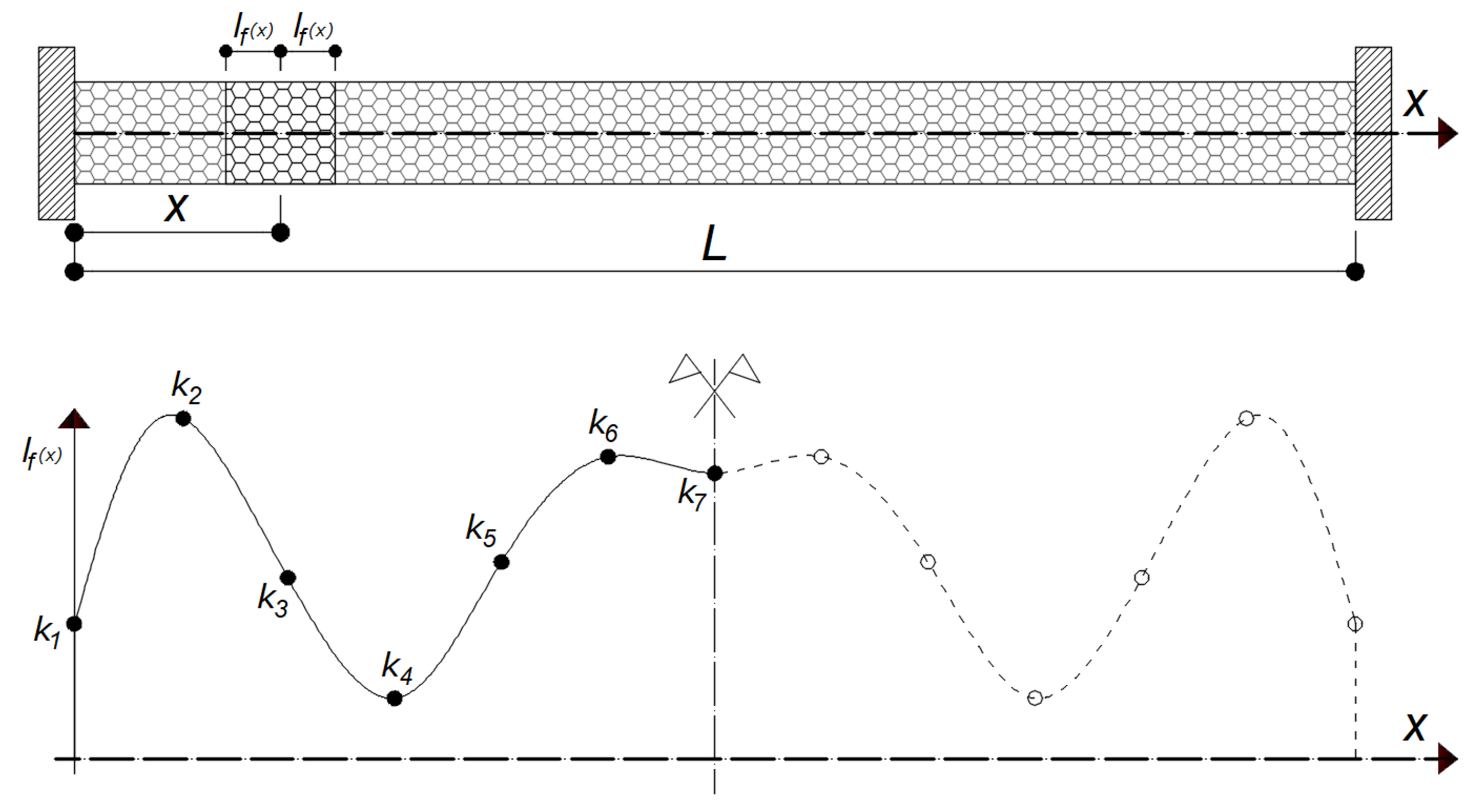
Aa mentioned 1D sFCM body fixed at both ends is analyzed (Figure 1). For the sake of simplicity, the non-dimensional case is considered, so L = 1 and for the fractional model , . Herein, as the maximum value of the length scale parameters in non-local theories are usually not larger than 10–20% of the macroscopic characteristic dimension of the structure; therefore, .
There are six control (“knot”) points, (cf. Figure 1), defining the length scale () distribution along the axis x, namely
For further analysis, we assume that vector denotes vector with components of value v. Next, the values between the knot points k are interpolated using cubic Hermite interpolator. Denoting the interpolator as , the length scale at point x can be expressed as follows:
According to the results obtained in [36], near to the ends of the structure, the length scale is linearly reduced from to . As a consequence, in the framework of the applied approximation, no information on displacements outside the body is required.
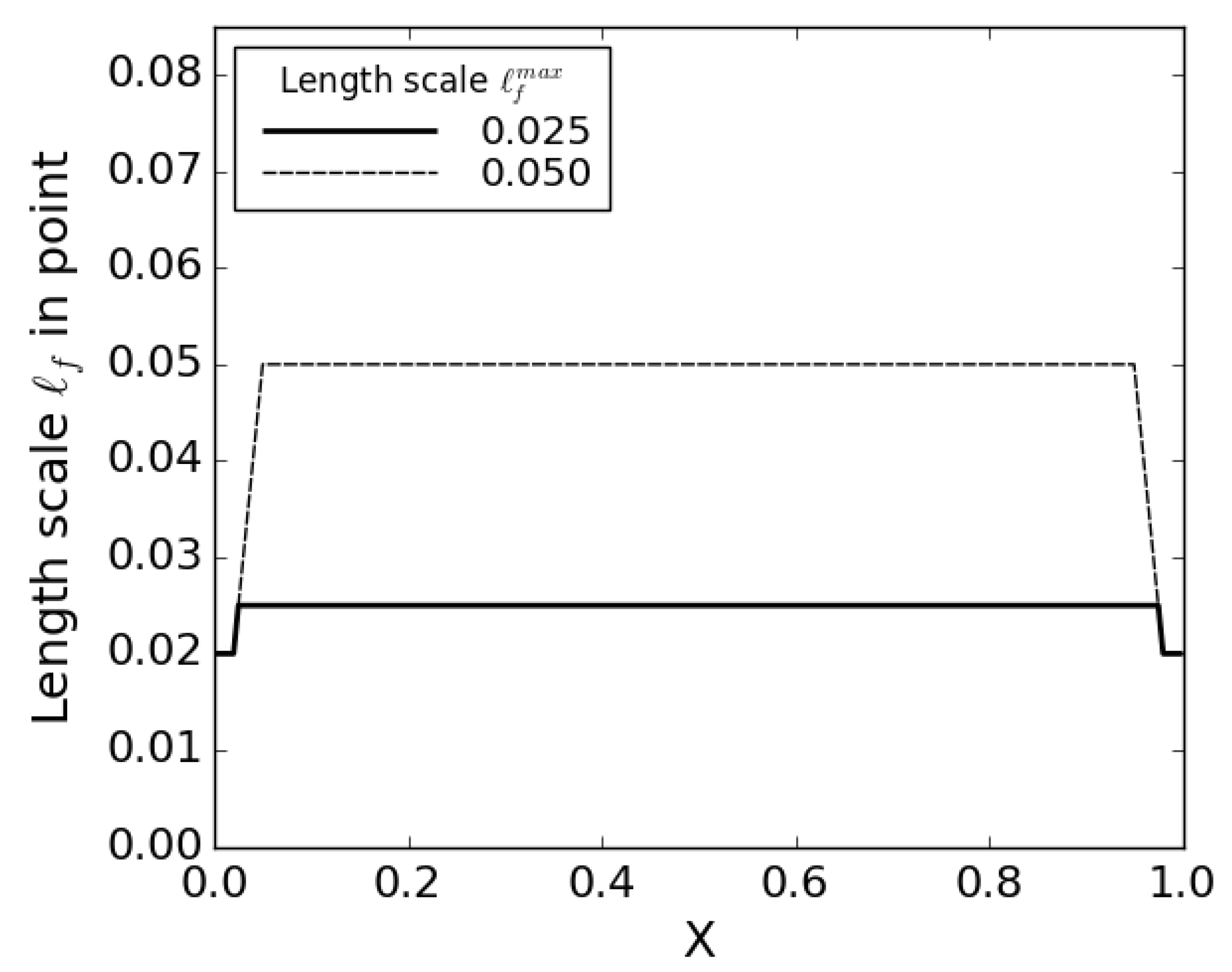
In the optimization procedure, the reduction of is carried out by application of the non-dimensional correction functional in a form
where is any function of class . As a result, the final function describing the length scale distribution can be defined in the following form
The graphical representation of function for the extreme case, i.e., is presented in Figure 2.
It is important, that model discretization depends on maximal length scale, namely for and for .
To solve the formulated optimization problem a dedicated procedure was developed in Python to build the global system of equations (Equation (11)). Due to the varied length scale, the governing equation for the particular points was built dynamically (cf. github.com/szajek) and the system of equations was solved using the LU decomposition [40] with partial pivoting and row interchanges.
3.2. Dynamic Response Evaluation
The dynamic response of the presented 1-D sFCM body is measured as a weighted sum of eigenvalues using Kreisselmeier–Steinhauser formula [33] in the form (the value of increases along with eigenvalues)
where and
The complexity of mode shape is limited by the size of underlying microstructure described by in the model. Moreover, as mentioned in the introduction, the wavelength limit is estimated by analogy to the spring-mass (discrete) structure [32]. Additionally, taking into account the inaccuracy due to the boundary condition application, the number of eigenvalues considered is limited based on the maximal length scale as follows:
The reference values of cumulative eigenvalues can be computed according to the equation
It should be noted that the values for a classical (local) model (when ) equal and .
3.3. Optimization Problem
The following optimization problem was formulated for each configuration of and :
where denotes the scaling parameter . The set of scale factors () for each configuration of (, ) was chosen from 1 to computed as follows:
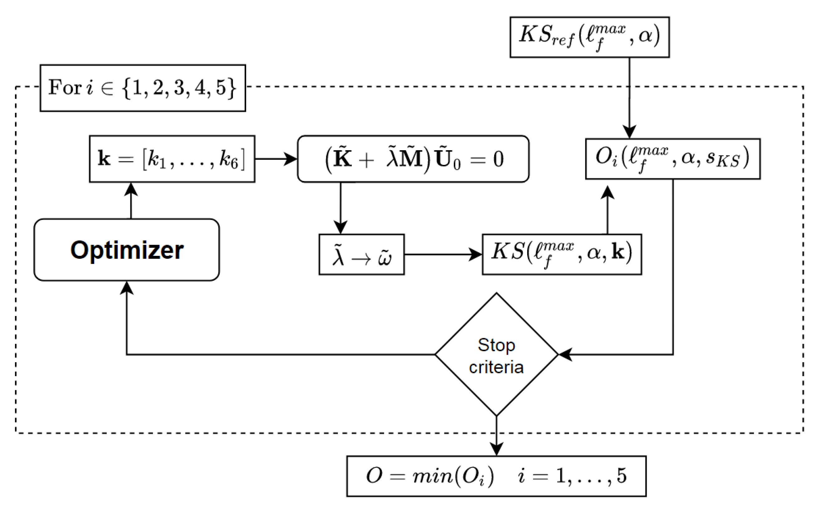
3.4. Algorithm
The problem described by Equation (20) was solved by coupling the computational model with an optimizer. The general overview of the procedure is presented in Figure 3. For a given and , the reference value of the weighted sum of eigenvalues is computed according to the Kreisselmeier–Steinhauser formula, . Next, the optimizer starts and iteratively propose vectors of values in control points, , which are a basis for model rebuilding—setting a length scale value for particular points along the body. The exact value of the length scale at point is calculated using Equations (13)–(15). Next, the eigenproblem is solved and the obtained eigenvalues are used to compute for the current length scale distribution. The difference between expected dynamic response (considering ) and the obtained one is computed according the objective function in Equation (20). For each configuration of and , the problem is solved five times and the solution characterized by the smallest value of the objective function is chosen.
The hybrid algorithm joining two optimization strategies was used, namely, a local search algorithm and an evolutionary algorithm. As a local search optimizer, the Limited-memory Broyden–Fletcher–Goldfarb–Shanno algorithm [41,42] implemented in the SciPy package was chosen. The evolutionary algorithm started with the initial population of 70 propositions (individuals—random values of ) and improved them by application of genetic operators. After seven iterations (generations) the best solution was set as a starting point for a local search procedure. The evolutionary strategy configuration was as follows: two-point crossover with a probability of 0.5, tournament selection with a group of three individuals, the Gaussian mutation of mean with a standard deviation of and probability . The mutation was applied for each parameter independently. The most important settings for local procedure are minimal relative change of an objective function—taken as (default value in the SciPy package), maximum number of iterations—taken as 15,000 and the step size for the numerical approximation of the Jacobian—taken as .
4. Results
The reference value of was computed according to Equation (19) for four values of and three values of . The results are collected in Table 1. The lowest values of are an effect of used discretization, namely, and for for and , respectively (cf. Section 3.1). Based on maximal values of scale factor was established according to Equation (21).
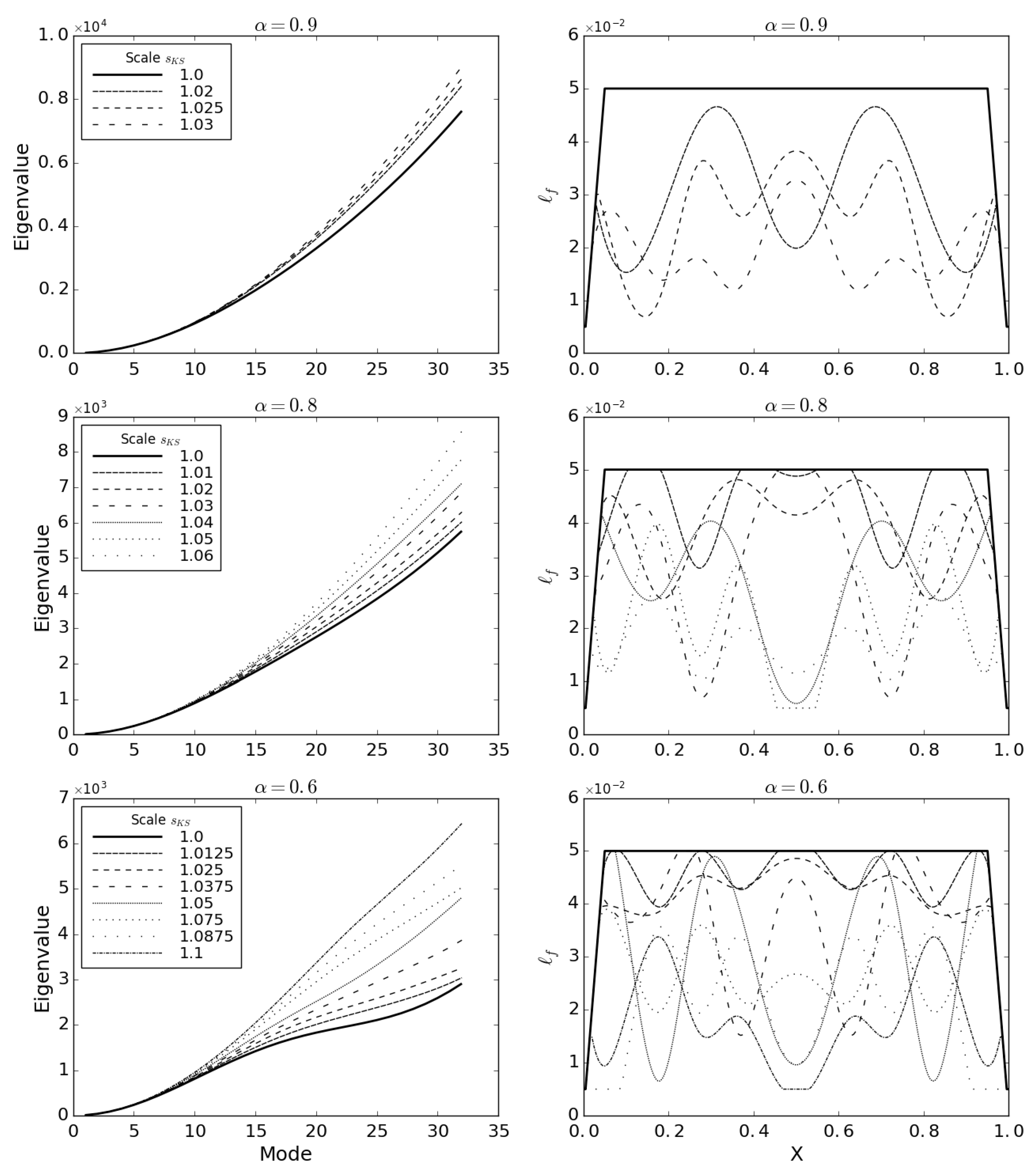
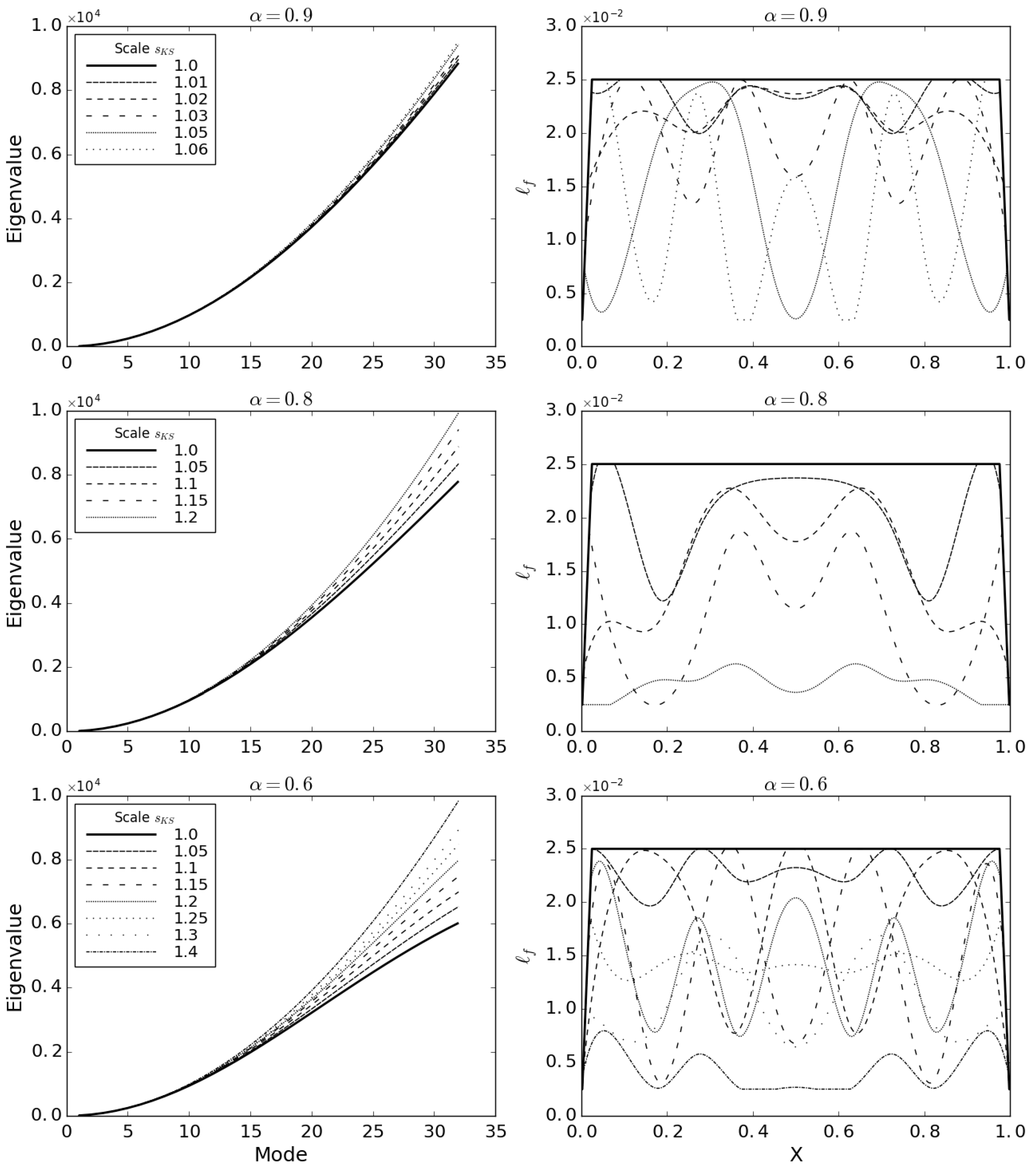
The optimization problem formulated in Equation (20) was solved for two values of , three values of and set of a scale factor . The optimization problem for each configuration of (, , ) was solved five times and the solution with the lowest objective function value was chosen. The best solutions—an objective value and parameters—are presented in Table 2 and Table 3. All obtained solutions are characterized by , which means that the expected dynamic behaviour was obtained with a high accuracy; the maximal error of 0.00385% was for , and . The total number of solved optimization problems equal ca. 200 with more than 130,000 single analyses (the calculations took several days—Intel Core i7-67000HQ, 16GB RAM). The results—eigenvalues spectra—are presented in Figure 4 and Figure 5.
Analysing the values and from Table 1, a few important observations can be made. First and foremost, the potential for modifying dynamic response by changing a length scale, measured as , depends on both: material order and the maximal permitted value of the length scale, . However, the role of due to a different number of considered eigenvalues is difficult to evaluate. Secondly, the value of , as it should be, tends to zero for the classical continuum model as . Finally, for all cases, as (dimensions of the body become considerably larger than the characteristic length scale), the solutions for a classical model are obtained independently on material order .
5. Conclusions
In this paper, the applicability of sFCM to design the material bodies with demanded dynamic eigenvalue spectrum is presented. The considered subject is meaningful both from the theoretical and practical points of view, especially when dealing with the design of sensors and actuators for nanotechnological applications, e.g., micro-thrusters of nano-satellites, torsional accelerometers, nano-motors or micro/nano-resonators. The problem is stated as a non-trivial inverse optimization task. As shown, different spectra are produced from different underlying microstructure distributions, which is described by the variable-length scale in the model. The obtained outcomes confirmed the correctness of our methodology, the optimization procedure and its implementation.
This in-depth study allows us to formulate the following conclusions:
- Designing the demanding dynamic response of a structure emphasising the scale effect by modifying length scale in the space-Fractional Continuum Mechanical model is possible;
- The potential for modifying dynamic response—measured as a weighted sum of eigenvalues—by changing a length scale is the biggest when the order of material continua and tends to zero for (the classical local model);
- The demanding dynamic response can be obtained by solving the inverse problem utilising hybridized optimization procedure joining the genetic and the limited-memory BFGS algorithms.
Author Contributions
Conceptualization, K.S. and W.S.; methodology, K.S. and W.S.; software, K.S.; validation, K.S., W.S., K.B. and T.B.; formal analysis, K.S. and W.S.; investigation, K.S. and W.S.; writing—original draft preparation, K.S. and W.S.; writing—review and editing, K.S. and W.S.; visualization, K.S.; supervision, W.S. and T.B.; project administration, W.S.; funding acquisition, W.S. All authors have read and agreed to the published version of the manuscript.
Funding
This research was funded by National Science Centre grant number 2017/27/B/ST8/00351.
Institutional Review Board Statement
Not applicable.
Conflicts of Interest
The authors declare no conflict of interest.
References
- Duan, H.; Wang, J.; Huang, Z.; Karihaloo, B. Size-dependent effective elastic constants of solids containing nano-inhomogeneities with interface stress. J. Mech. Phys. Solids 2005, 53, 1574–1596. [Google Scholar] [CrossRef]
- Li, Y.; Wei, P.; Tang, Q. Reflection and transmission of elastic waves at the interface between two gradient-elastic solids with surface energy. Eur. J. Mech. A/Solids 2015, 52, 54–71. [Google Scholar] [CrossRef] [Green Version]
- Miller, R.E.; Shenoy, V.B. Size-dependent elastic properties of nanosized structural elements. Nanotechnology 2000, 11, 139–147. [Google Scholar] [CrossRef]
- Zhang, L.; Guo, J.; Xing, Y. Nonlocal analytical solution of functionally graded multilayered one-dimensional hexagonal piezoelectric quasicrystal nanoplates. Acta Mech. 2019, 230, 1781–1810. [Google Scholar] [CrossRef]
- Barretta, R.; Faghidian, S.A.; Marotti de Sciarra, F. Aifantis versus Lam strain gradient models of Bishop elastic rods. Acta Mech. 2019, 230, 2799–2812. [Google Scholar] [CrossRef]
- Liu, D.; Tarakanova, A.; Hsu, C.C.; Yu, M.; Zheng, S.; Yu, L.; Liu, J.; He, Y.; Dunstan, D.J.; Buehler, M.J. Spider dragline silk as torsional actuator driven by humidity. Sci. Adv. 2019, 5, eaau9183. [Google Scholar] [CrossRef] [Green Version]
- Heinisch, M.; Voglhuber-Brunnmaier, T.; Reichel, E.; Dufour, I.; Jakoby, B. Electromagnetically driven torsional resonators for viscosity and mass density sensing applications. Sens. Actuators A Phys. 2015, 229, 182–191. [Google Scholar] [CrossRef] [Green Version]
- Lam, J.K.; Koay, S.C.; Lim, C.H.; Cheah, K.H. A voice coil based electromagnetic system for calibration of a sub-micronewton torsional thrust stand. Measurement 2019, 131, 597–604. [Google Scholar] [CrossRef]
- Xiao, D.; Xia, D.; Li, Q.; Hou, Z.; Liu, G.; Wang, X.; Chen, Z.; Wu, X. A double differential torsional accelerometer with improved temperature robustness. Sens. Actuators A Phys. 2016, 243, 43–51. [Google Scholar] [CrossRef]
- Dang, V.H.; Nguyen, D.A.; Le, M.Q.; Duong, T.H. Nonlinear vibration of nanobeams under electrostatic force based on the nonlocal strain gradient theory. Int. J. Mech. Mater. Des. 2020, 16, 289–308. [Google Scholar] [CrossRef]
- Patnaik, S.; Hollkamp, J.; Semperlotti, F. Applications of variable-order fractional operators: A review. Proc. R. Soc. A Math. Phys. Eng. Sci. 2020, 476. [Google Scholar] [CrossRef] [PubMed] [Green Version]
- Lazopoulos, A.K. On fractional peridynamic deformations. Arch. Appl. Mech. 2016, 86, 1987–1994. [Google Scholar] [CrossRef]
- Postek, E.; Pecherski, R.; Nowak, Z. Peridynamic Simulation of Crushing Processes in Copper Open-Cell Foam. Arch. Metall. Mater. 2019, 64, 1603–1610. [Google Scholar]
- Eringen, A. On differential equations of nonlocal elasticity and solutions of screw dislocations and surface waves. J. Appl. Phys. 1983, 54, 4703–4710. [Google Scholar] [CrossRef]
- Peddieson, J.; Buchanan, G.; McNitt, R. The role of strain gradients in the grain size effect for polycrystals. Int. J. Eng. Sci. 2003, 41, 305–312. [Google Scholar] [CrossRef]
- Eringen, A. Nonlocal Continuum Field Theories; Springer: New York, NY, USA, 2010. [Google Scholar]
- Toupin, R. Elastic materials with couple-stress. Arch. Ration. Mech. Anal. 1962, 11, 385–414. [Google Scholar] [CrossRef] [Green Version]
- Mindlin, R.; Eshel, N. On first strain-gradient theories in linear elasticity. Int. J. Solids Struct. 1968, 4, 109–124. [Google Scholar] [CrossRef]
- Aifantis, E. On the Microstructural Origin of Certain Inelastic Models. J. Eng. Mater. Technol. (ASME) 1984, 106, 326–330. [Google Scholar] [CrossRef]
- Li, J.; Wang, B. Fracture mechanics analysis of an anti-plane crack in gradient elastic sandwich composite structures. Int. J. Mech. Mater. Des. 2019, 15, 507–519. [Google Scholar] [CrossRef]
- Cosserat, E.; Cosserat, F. Theorie des Corps Deformables; Librairie Scientifique A. Hermann et Fils: Paris, France, 1909. [Google Scholar]
- Eringen, A. Linear Theory of Micropolar Elasticity. J. Math. Mech. 1966, 15, 909–923. [Google Scholar]
- Nowacki, W. Theory of Micropolar Elasticity; CISM: Udine, Italy, 1972. [Google Scholar]
- Gurtin, M.; Murdoch, A. A Continuum Theory of Elastic Material Surfaces. Arch. Ration. Mech. Anal. 1975, 57, 291–323. [Google Scholar] [CrossRef]
- Drapaca, C.; Sivaloganathan, S. Brief Review of Continuum Mechanics Theories. Fields Inst. Monogr. 2019, 37, 5–37. [Google Scholar]
- Sumelka, W. Thermoelasticity in the Framework of the Fractional Continuum Mechanics. J. Therm. Stress. 2014, 37, 678–706. [Google Scholar] [CrossRef]
- Podlubny, I. Fractional Differential Equations; Mathematics in Science and Engineering; Academin Press: Cambridge, MA, USA, 1999; Volume 198. [Google Scholar]
- Kilbas, A.; Srivastava, H.; Trujillo, J. Theory and Applications of Fractional Differential Equations; Elsevier: Amsterdam, The Netherlands, 2006. [Google Scholar]
- Malinowska, A.; Odzijewicz, T.; Torres, D. Advanced Methods in the Fractional Calculus of Variations; Springer Briefs in Applied Sciences and Technology; Springer: Berlin/Heidelberg, Germany, 2015. [Google Scholar]
- Sumelka, W.; Blaszczyk, T.; Liebold, C. Fractional Euler–Bernoulli beams: Theory, numerical study and experimental validation. Eur. J. Mech. A/Solids 2015, 54, 243–251. [Google Scholar] [CrossRef] [Green Version]
- Stempin, P.; Sumelka, W. Space-fractional Euler-Bernoulli beam model—Theory and identification for silver nanobeam bending. Int. J. Mech. Sci. 2020, 186, 105902. [Google Scholar] [CrossRef]
- Szajek, K.; Sumelka, W. Discrete mass-spring structure identification in nonlocal continuum space-fractional model. Eur. Phys. J. Plus 2019, 134, 448. [Google Scholar] [CrossRef] [Green Version]
- Kreisselmeier, G.; Steinhauser, R. Systematic Control Design by Optimizing a Vector Performance Index. In Proceedings of the IFAC Symposium on computer Aided Design of Control Systems, Zurich, Switzerland, 29–31 August 1979; Volume 12, pp. 113–117. [Google Scholar] [CrossRef]
- Sumelka, W.; Zaera, R.; Fernández-Sáez, J. A theoretical analysis of the free axial vibration of non-local rods with fractional continuum mechanics. Meccanica 2015, 50, 2309–2323. [Google Scholar] [CrossRef] [Green Version]
- Sumelka, W.; Zaera, R.; Fernández-Sáez, J. One-dimensional dispersion phenomena in terms of fractional media. Eur. Phys. J. Plus 2016, 131, 320. [Google Scholar] [CrossRef] [Green Version]
- Sumelka, W. On fractional non-local bodies with variable length scale. Mech. Res. Commun. 2017, 86, 5–10. [Google Scholar] [CrossRef]
- Hall, F.; Hayhurst, D. Modelling of Grain Size Effects in Creep Crack Growth Using a Non-Local Continuum Damage Approach. Proc. Math. Phys. Sci. 1991, 433, 405–421. [Google Scholar]
- Peerlings, R.; Geers, M.; de Borst, R.; Brekelmans, W. A critical comparison of nonlocal and gradient-enhanced softening continua. Int. J. Solids Struct. 2001, 38, 7723–7746. [Google Scholar] [CrossRef]
- Szajek, K.; Sumelka, W.; Blaszczyk, T.; Bekus, K. On selected aspects of space-fractional continuum mechanics model approximation. Int. J. Mech. Sci. 2020, 167, 105287. [Google Scholar] [CrossRef]
- Strang, G. Linear Algebra and Its Applications, 2nd ed.; Academic Press Inc.: Orlando, FL, USA, 1980. [Google Scholar]
- Byrd, R.H.; Lu, P.; Nocedal, J.; Zhu, C. A Limited Memory Algorithm for Bound Constrained Optimization. SIAM J. Sci. Stat. Comput. 1995, 16, 1190–1208. [Google Scholar] [CrossRef]
- Zhu, C.; Byrd, R.H.; Lu, P.; Nocedal, J. L-BFGS-B, FORTRAN routines for large scale bound constrained optimization. ACM Trans. Math. Softw. 1997, 23, 550–560. [Google Scholar] [CrossRef]
Figure 1.
General scheme and length scale parameterization: (top) 1D space-fractional non-local formulation (sFCM) body of length L fixed at both ends; (bottom) spatial length scale distribution through 1D sFCM body.
Figure 1.
General scheme and length scale parameterization: (top) 1D space-fractional non-local formulation (sFCM) body of length L fixed at both ends; (bottom) spatial length scale distribution through 1D sFCM body.

Figure 2.
Limit spatial length scale distributions through 1D sFCM body () for two analysed variants.
Figure 2.
Limit spatial length scale distributions through 1D sFCM body () for two analysed variants.

Figure 3.
General workflow of the optimization procedure.

Figure 4.
Eigenvalues (left column) and corresponding length scale distributions (right column) for particular material orders and .
Figure 4.
Eigenvalues (left column) and corresponding length scale distributions (right column) for particular material orders and .

Figure 5.
Eigenvalues (left column) and corresponding length scale distributions (right column) for particular material orders and .
Figure 5.
Eigenvalues (left column) and corresponding length scale distributions (right column) for particular material orders and .


Table 1.
Reference value of and for various combination of maximal length scale and material order .
Table 1.
Reference value of and for various combination of maximal length scale and material order .
| 0.05 | 0.025 | 0.005 | 0.0025 | 0.05 | 0.025 | ||||
|---|---|---|---|---|---|---|---|---|---|
| 0.9 | 390.5 | 994.6 | 405.1 | 1096.2 | 0.9 | 1.04 | 1.10 | ||
| 0.8 | 378.2 | 907.3 | 404.8 | 1094.3 | 0.8 | 1.07 | 1.21 | ||
| 0.6 | 358.9 | 772.1 | 404.4 | 1091.4 | 0.6 | 1.13 | 1.41 | ||
Table 2.
Objective value and parameters for the best solutions: length scale and .
| O | Parameters k | ||||||||
|---|---|---|---|---|---|---|---|---|---|
| 0.025 | 0.6 | 1 | 5.95 | 2.50 | 2.50 | 2.50 | 2.50 | 2.50 | 2.50 |
| 1.05 | 8.97 | 2.41 | 2.22 | 2.00 | 2.50 | 2.22 | 2.29 | ||
| 1.1 | 1.74 | 2.50 | 2.27 | 2.43 | 1.78 | 7.84 | 2.23 | ||
| 1.15 | 7.88 | 6.50 | 1.97 | 3.14 | 1.63 | 2.48 | 9.95 | ||
| 1.2 | 1.00 | 1.54 | 1.81 | 8.08 | 1.85 | 7.54 | 1.76 | ||
| 1.25 | 2.01 | 2.25 | 1.29 | 1.41 | 1.51 | 1.35 | 1.40 | ||
| 1.3 | 3.17 | 9.60 | 7.29 | 8.83 | 1.62 | 1.46 | 7.67 | ||
| 1.4 | 1.19 | 3.23 | 6.64 | 2.59 | 5.78 | 2.74 | 2.50 | ||
| 0.8 | 1 | 2.47 | 2.50 | 2.50 | 2.50 | 2.50 | 2.50 | 2.50 | |
| 1.05 | 2.01 | 1.41 | 2.35 | 1.23 | 1.87 | 2.29 | 2.36 | ||
| 1.1 | 1.28 | 4.76 | 1.01 | 1.03 | 1.93 | 2.26 | 1.86 | ||
| 1.15 | 1.95 | 2.37 | 6.52 | 2.50 | 8.64 | 1.87 | 1.30 | ||
| 1.2 | 3.14 | 2.50 | 3.04 | 4.77 | 4.80 | 6.29 | 4.14 | ||
| 0.9 | 1 | 3.23 | 2.50 | 2.50 | 2.50 | 2.50 | 2.50 | 2.50 | |
| 1.01 | 8.94 | 2.50 | 2.50 | 2.50 | 1.99 | 2.39 | 2.35 | ||
| 1.02 | 1.60 | 1.36 | 2.10 | 2.16 | 2.02 | 2.39 | 2.39 | ||
| 1.03 | 2.44 | 7.54 | 2.44 | 2.07 | 1.37 | 2.47 | 1.80 | ||
| 1.05 | 5.18 | 9.02 | 6.43 | 1.97 | 2.43 | 2.17 | 5.65 | ||
| 1.06 | 2.21 | 1.54 | 1.75 | 5.14 | 2.37 | 2.50 | 1.24 | ||
Table 3.
Objective value and parameters for the best solutions: length scale and .
| O | Parameters k | ||||||||
|---|---|---|---|---|---|---|---|---|---|
| 0.05 | 0.6 | 1 | 1.47 | 5.00 | 5.00 | 5.00 | 5.00 | 5.00 | 5.00 |
| 1.0125 | 1.21 | 1.61 | 4.96 | 3.94 | 5.00 | 4.28 | 4.97 | ||
| 1.025 | 6.82 | 3.53 | 3.90 | 3.87 | 4.53 | 4.29 | 4.75 | ||
| 1.0375 | 1.39 | 4.46 | 3.70 | 4.28 | 4.84 | 1.55 | 3.85 | ||
| 1.05 | 4.99 | 3.06 | 4.21 | 6.63 | 4.35 | 3.99 | 1.40 | ||
| 1.075 | 1.67 | 1.71 | 3.42 | 1.97 | 3.59 | 2.25 | 2.52 | ||
| 1.0875 | 2.57 | 5.01 | 6.01 | 3.57 | 1.93 | 3.40 | 1.46 | ||
| 1.1 | 2.79 | 2.67 | 1.64 | 3.37 | 1.56 | 1.88 | 6.54 | ||
| 0.8 | 1 | 1.63 | 5.00 | 5.00 | 5.00 | 5.00 | 5.00 | 5.00 | |
| 1.01 | 1.99 | 2.87 | 4.76 | 5.00 | 3.14 | 4.91 | 4.98 | ||
| 1.02 | 2.63 | 1.92 | 4.25 | 2.56 | 3.91 | 4.81 | 4.27 | ||
| 1.03 | 2.34 | 2.66 | 3.94 | 3.67 | 7.17 | 3.02 | 4.95 | ||
| 1.04 | 1.58 | 5.00 | 3.17 | 2.62 | 3.91 | 3.32 | 1.00 | ||
| 1.05 | 2.38 | 5.00 | 1.78 | 3.94 | 1.48 | 3.20 | 5.00 | ||
| 1.06 | 1.46 | 2.33 | 1.70 | 2.57 | 1.05 | 1.98 | 1.35 | ||
| 0.9 | 1 | 1.08 | 5.00 | 5.00 | 5.00 | 5.00 | 5.00 | 5.00 | |
| 1.02 | 6.99 | 4.29 | 1.55 | 2.57 | 4.39 | 4.26 | 2.34 | ||
| 1.025 | 1.19 | 3.69 | 1.38 | 1.09 | 3.60 | 2.60 | 3.54 | ||
| 1.03 | 1.08 | 9.70 | 2.50 | 1.38 | 1.80 | 1.21 | 2.89 | ||
Publisher’s Note: MDPI stays neutral with regard to jurisdictional claims in published maps and institutional affiliations. |
© 2021 by the authors. Licensee MDPI, Basel, Switzerland. This article is an open access article distributed under the terms and conditions of the Creative Commons Attribution (CC BY) license (http://creativecommons.org/licenses/by/4.0/).
Share and Cite
MDPI and ACS Style
Szajek, K.; Sumelka, W.; Bekus, K.; Blaszczyk, T. Designing of Dynamic Spectrum Shifting in Terms of Non-Local Space-Fractional Mechanics. Energies 2021, 14, 506. https://0-doi-org.brum.beds.ac.uk/10.3390/en14020506
AMA Style
Szajek K, Sumelka W, Bekus K, Blaszczyk T. Designing of Dynamic Spectrum Shifting in Terms of Non-Local Space-Fractional Mechanics. Energies. 2021; 14(2):506. https://0-doi-org.brum.beds.ac.uk/10.3390/en14020506
Chicago/Turabian StyleSzajek, Krzysztof, Wojciech Sumelka, Krzysztof Bekus, and Tomasz Blaszczyk. 2021. "Designing of Dynamic Spectrum Shifting in Terms of Non-Local Space-Fractional Mechanics" Energies 14, no. 2: 506. https://0-doi-org.brum.beds.ac.uk/10.3390/en14020506
Note that from the first issue of 2016, this journal uses article numbers instead of page numbers. See further details here.